Promotion of Green Technology under Different Environmental Policies

Abstract

In this paper, I develop a two-stage game of pollution abatement technology adoption in a Cournot oligopoly to investigate a firm’s decision to adopt pollution abatement technology. In particular, I study the adoption incentives and welfare implications of popular environmental policies, namely emission fees and quotas. Tradeable permits result in identical outcomes to emission fees. Within each policy regime, the conditions for Nash equilibria are identified where both firms invest in the green technology, neither firm invests in the technology, or only one firm invests. The following extensions are also analyzed: asymmetric adoption costs, increase in the marginal cost of production from adoption, and a type-dependent fee where adoption reduces the emission fee. Social welfare under an emission fee is identical to that under a quota. However, when policy is (not) stringent, firms are more willing to adopt expensive technology under a fee (quota) than under a quota (fee, respectively).

1. Introduction

About seven million premature deaths (one in eight total deaths worldwide) are attributed to air pollution.1 One way to mitigate this damage is through more environmentally friendly (“green”) production processes. Green technology can reduce emissions from production through the use of green energy, electric vehicles, carbon capture storage and usage, and other abatement technologies that reduce pollution from production of a good. An example of a green technology is that of new techniques to dye textiles with significantly less water.2 New waterless dyeing techniques use significantly less water, dye, and energy, leading to a lower environmental impact. However, the adoption of this new technology has been slow because of the significant initial adoption costs.

The adoption of these technologies in an entire industry follows an S-shaped curve. When the technology is in its infancy, adoption is slow. As more and more firms adopt the technology, the rate of adoption speeds up until it is almost universally adopted and the growth of adoption slows again (see Kemp and Volpi [1], for a more extensive discussion). If green technology is available in an industry, it may be in society’s best interest for the regulator to promote the use of this technology through policy. This paper takes an extensive look at the social welfare implications under different environmental policies that aim to promote green technology adoption in order to provide policy makers with the best approach to this problem.

A number of policies can encourage the adoption of green technology through the firm’s incentive to reduce compliance costs. I consider the following: an emissions fee, a type-dependent fee that reduces the existing emissions fee if the technology is adopted, tradeable permits (cap-and-trade), or an emissions quota. For each, I evaluate which policy leaves society in the best situation possible based on social welfare, and how firm incentives align with that ranking. I also evaluate these policies under adoption cost asymmetries and when adoption increases the marginal cost of production.

Much of the literature focuses on how policies impact a firm’s incentive to innovate and the effects on social cost largely ignoring changes in consumer surplus resulting from changes in firm output (see [2,3,4,5,6,7,8,9]). The consensus in the literature is that market based policies outperform command-and-control policies in minimizing social costs. Looking solely at the social cost, i.e., environmental damage and adoption costs, ignores any changes in the firms’ compliance costs, which could affect equilibrium quantity and price. The literature largely assumes a case where all, or many, of the firms operating in the market adopt the technology. This paper examines a setting in which each firm in a Cournot duopoly chooses to adopt or not adopt the technology, including an equilibrium where only one firm will adopt the technology.

Amacher and Malik [10] study technology adoption in the context of an emission fee on how the decision changes based on whether the regulator commits to a tax either before or after the adoption decision. The focus in Amacher and Malik is on social costs (adoption costs plus damages), not social welfare as a whole. Requate [11] looks at the social welfare under implications of innovation under taxes and tradeable permits under an N-firm Bertrand competition finding that permits create a more efficient market than taxes. In contrast, I study a duopoly’s decision to adopt technology under these policies (and more) identifying what situations facilitate adoption, and the effect on social welfare.

A number of papers investigate adoption decisions of production cost-reducing technology under a number of different circumstances while using a static adoption game. Jensen [12] uses this type of game to analyze how uncertainty of the effectiveness of the new technology impacts the adoption decision of two firms. Following Jensen’s approach, Zhang et al. [13] investigate how many firms choose to adopt such a technology in an N-firm Cournot model in the presence of knowledge spillovers. Pal [14] compares the adoption incentives to invest under Cournot and Bertrand competition. The present model uses a similar approach to the aforementioned papers in order to compare the incentives to invest, however I consider emissions reducing technology under different environmental policies.3

The type of game studied here draws some parallels to that of the binary-contribution threshold public goods games literature first studied theoretically by Palfrey and Rosenthal [19] and Diekmann [20]. More closely related to the present model is the experiment studying green power programs by Rose et al. [21]. However, the present paper models the benefit from contributing (investing in the abatement technology) as being realized by society as a whole through having more of the good available at a given emissions level. The free-rider problem is not significant, as non-adopting firms are actually at a cost disadvantage in the case of an emission fee as the fee per unit produced is higher than if they had adopted the technology.4 In the case of a quota, the adopting firm is able to produce more under the same level of emissions as the non-adopting firm.

I find that, under equivalent resulting emissions, social welfare coincides under a fee and quota; however, firm profits are lower under an emission fee. Firms prefer to face a quota rather than an equivalent fee as an emission fee increases each firm’s marginal cost and, thus, lowers their profit as compared to if the firm was subject to a quota. A type-dependent fee increases firm profits compared to the uniform fee since the adopting firm pays a decreased fee on their emissions, but it does not result in greater profits than under a quota. Because profits under the quota are higher, firms are more willing to adopt a more expensive technology under the quota. If the goal of the regulator is to encourage the adoption of abatement technologies, especially costly technologies, the regulator would more likely achieve this goal under a quota than under a fee.

2. Results

To evaluate the social welfare implications of the various policies, I use a two-stage technology adoption game with two firms competing à la Cournot in each stage. In the first stage, each firm decides whether or not to adopt a green technology, and the firms compete over quantities.5 Firms are not able to realize the benefits of the adopted technology in the first stage; thus, they are unable to use this technology to abate their emissions. In the second stage, the firms compete over quantity, but lower emissions if they chose to adopt the green technology when compared to if they do not adopt the technology. First, I solve the case where there is a per-unit tax on emissions. Once this case is established, I evaluate tradeable permits and quotas.

2.1. Emission Fee

In the first stage, each firm decides whether or not to invest in the green technology. If it invests, it pays a one time fee to incorporate and install the technology into the firm’s production process of $Z_k>0$, where $k=\{i,j\}$ indicates the firm, and $Z_i$ and $Z_j$ can differ depending on the firm’s ability to incorporate the technology into their production process. I first assume that $Z_i=Z_j=Z$, but later relax this assumption.6

In the second stage, the two firms independently maximize their profits by choosing quantity $q_k$. Firms face the same linear inverse demand $P=a-Q$ where P is the price, $a>0$, and $Q=q_i+q_j$ is total production. Each firm produces the good at constant marginal cost c, where $a>c>0$, and emissions are $e_k=\gamma q_k$, where $\gamma >0$ represents emissions per unit produced. If the firm invested in the green technology, per unit emissions are reduced by $\alpha$ to $e_k=(\gamma -\alpha )q_k$ where $\gamma >\alpha >0$. The environmental damage function is $d{E}^2$, where $d>0$ is a measure of environmental damage and $E=e_i+e_j$ is the total amount of emissions from production. In the baseline case, each firm pays the same emissions fee t.7 I assume that $t<\frac{a-c}{\gamma +\alpha }$ so that firms produce positive quantities when they do not invest in the technology.

The game is solved using backward induction. First, firms simultaneously maximize profits in the second stage by choosing quantity, taking both their and their rival’s investment decision in the first stage as given. In the first stage, each firm chooses quantity in order to maximize profit and whether or not to purchase the green technology in order to maximize second stage profits.8 Given these potential profits and adoption decision of their rival, firms then decide to adopt or not adopt the technology in the first stage.

In the second stage, firms face two potential profit functions depending on the adoption of technology in the first stage. Second stage profit for firm i, if it does not invest in the green technology, when there is an emissions fee is

$${\Pi }_i^{NI}=(a-(q_i+q_j))q_i-c{q}_i-t\gamma q_i,$$

where the “NI” superscript represents “not investing” in the new technology. The first-order condition for firm i is

$${\displaystyle \frac{\partial {\Pi }_i^{NI}}{\partial q_i}}=a-q_j-2q_i-(c+t\gamma )=0,$$

and the best-response function is $q_i\left(q_j\right)={\displaystyle \frac{a-c-t\gamma }{2}}-{\displaystyle \frac{1}{2}}{q}_j$, which the firm uses regardless of the investment decision of the other firm.

If firm i chooses to invest in the green technology, its profits in the second stage are

$${\Pi }_i^{INV}=(a-(q_i+q_j))q_i-c{q}_i-t(\gamma -\alpha )q_i,$$

where the superscript “INV” represents the case where the firm “invests” in the new technology. In this case, the firm i’s first-order condition is

$${\displaystyle \frac{\partial {\Pi }_i^{INV}}{\partial q_i}}=a-q_j-2q_i-(c+t(\gamma -\alpha ))=0,$$

with best-response function $q_i\left(q_j\right)={\displaystyle \frac{a-c-t(\gamma -\alpha )}{2}}-{\displaystyle \frac{1}{2}}{q}_j$.

The two response functions define four sets of equilibrium quantities and profits: (1) neither firm invests, (2) both firms invest, and (3) and (4) one firm invests and the other does not invest.

Table 1. Equilibrium quantity and profit in the baseline emission fee.

	Quantity	Profit
Neither firm invests	$q_i=\frac{1}{3}(a-c-\gamma t)$	${\Pi }_i^{NI,NI}=\frac{1}{9}{(a-c-t\gamma )}^2$
Both firms invest	$q_i=\frac{1}{3}(a-c-t(\gamma -\alpha ))$	${\Pi }_i^{INV,INV}=\frac{1}{9}{(a-c-t(\gamma -\alpha ))}^2$
Firm i invests, firm j does not	$q_i=\frac{1}{3}(a-c-t(\gamma -2\alpha ))$	${\Pi }_i^{INV,NI}=\frac{1}{9}{(a-c-t(\gamma -2\alpha ))}^2$
Firm j invests, firm i does not	$q_i=\frac{1}{3}(a-c-t(\gamma +\alpha ))$	${\Pi }_i^{NI,INV}=\frac{1}{9}{(a-c-t(\gamma +\alpha ))}^2$

presents the corresponding quantities and profits for firm i in each case. In the superscript on profit, $\Pi$, the first abbreviation denotes that firm’s investment decision, while the second denotes its opponent’s investment decision. For example, ${\Pi }^{INV,NI}$ is firm i’s profit when it invests in the technology, while its opponent does not invest in the technology.

In the first stage, each firm decides whether or not to invest in the green technology while taking the resulting profit in the second stage and the cost of the investment into account.

Table 2. Normal form representation of the game.

		Firm j
		Invest	No Invest
Firm i	Invest	${\Pi }_i^{INV,INV}-Z,{\Pi }_j^{INV,INV}-Z$	${\Pi }_i^{INV,NI}-Z,{\Pi }_j^{NI,INV}$
	No Invest	${\Pi }_i^{NI,INV},{\Pi }_j^{INV,NI}-Z$	${\Pi }_i^{NI,NI},{\Pi }_j^{NI,NI}$

shows the firm’s decision to invest is based on the two-by-two game.

The following proposition presents the Nash equilibrium in the case of the emission fee.9

Proposition 1.

In the case of an emission fee, the equilibrium adoption decisions are:

1. 

Both firms adopt the technology if $Z<\frac{1}{9}\left(4t\alpha (a-c-t\gamma )\right)$.

2. 

Neither firm adopts the technology if $Z>\frac{1}{9}(4t\alpha (a-c-t(\gamma -\alpha ))$.

3. 

Only one firm adopts the technology if $\frac{1}{9}\left(4t\alpha (a-c-t\gamma )\right)<Z<\frac{1}{9}\left(4t\alpha (a-c-t(\gamma -\alpha ))\right)$.10

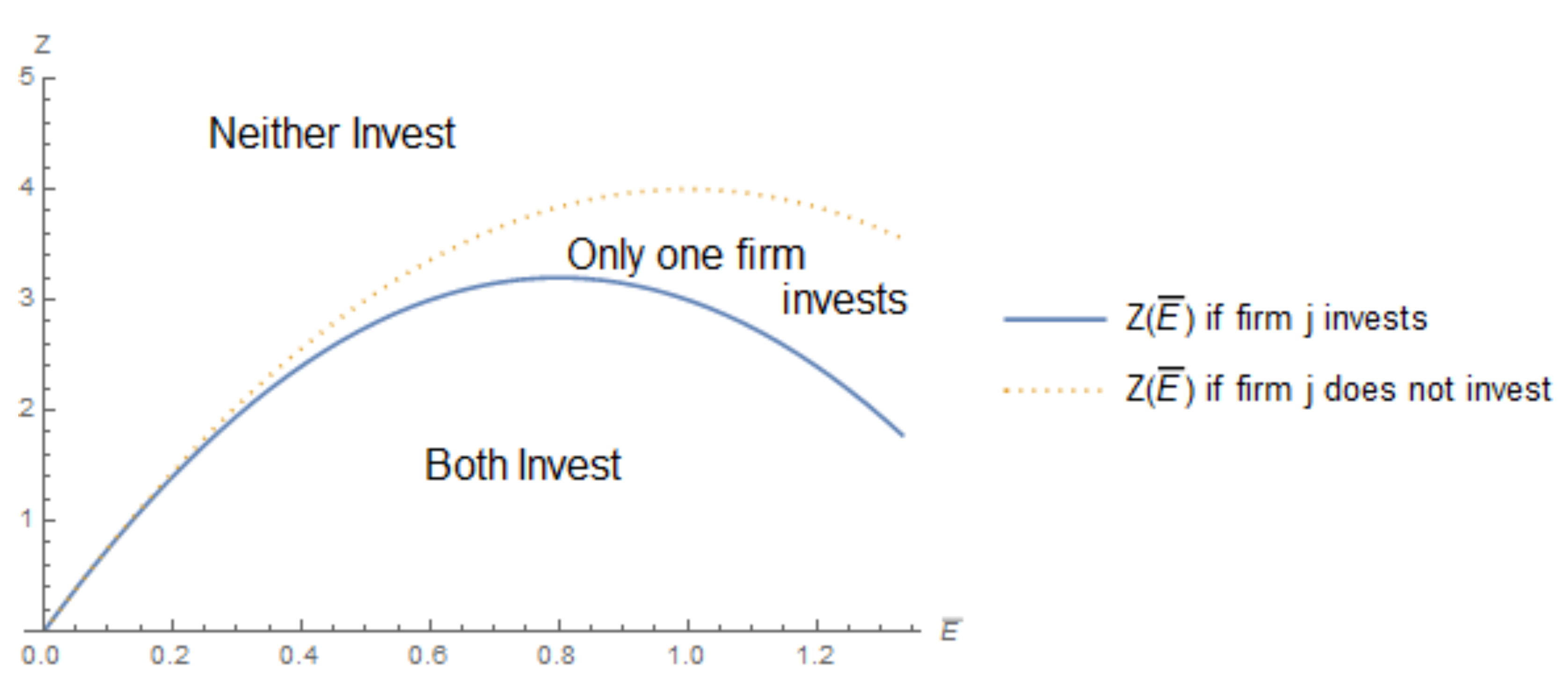
When the cost of investment is too high, neither firm invests in the green technology. However, if the cost of investment is low, then both of the firms choose to invest in the technology. Between the two adoption cost cutoffs, the equilibrium conditions predict that only one firm invests.

Figure 1 shows the regions on the cost of investment in which a firm invests in the technology, as described in Proposition 1, dependent on the emission fee and the opposing firm’s adoption decision, denoted as $Z\left(t\right)$.11 If there is no emission fee, there is no incentive to adopt the green technology, as there is no other benefit to the green technology outside of reducing compliance costs, and firms will be indifferent in adopting the technology if it comes at zero cost. If the fee is low, the reduction in pollution does not result in a significant decrease in the firm’s marginal costs and, hence, the cost of the green technology must be low. As the tax increases, the firm is willing to pay more for the green technology. When the tax becomes more stringent and the resulting profits become smaller, the investment cost must also decrease for the adoption to be the optimal strategy.12

Next, this process is repeated under a quota, and then the investment decisions, social welfare, and profits are compared. Starting in Section 2.4, different extensions are explored under each policy.

2.2. Quota

Next, I investigate the equilibria when there is an emissions quota. The quota acts as an upper bound on individual firm emissions at the level of $\overline{E}$. If the quota is not binding, then the firms will act as though there is no regulation and there will be no incentive to adopt the technology. Therefore, the emission quota is set so that it is binding. Solving $\overline{E}=q_k{e}_k$, each firm k chooses $q_k=\frac{\overline{E}}{\gamma }$ if the firm does not invest in the abatement technology and $q_k=\frac{\overline{E}}{\gamma -\alpha }$ if it does invest in the abatement technology.13 The Nash equilibria are summarized in the following proposition using the same strategy as the fee.

Proposition 2.

In the case of a quota, the equilibrium adoption decisions are:

1. 

Both firms adopt the technology if $Z<\frac{\overline{E}\alpha (\gamma (a-c)(\gamma -\alpha )-\overline{E}(3\gamma -\alpha ))}{{(\gamma -\alpha )}^2{\gamma }^2}$.

2. 

Neither firm adopts the technology if $Z>\frac{\overline{E}\alpha (\gamma (a-c)(\gamma -\alpha )-\overline{E}(3\gamma -2\alpha ))}{{(\gamma -\alpha )}^2{\gamma }^2}$.

3. 

Only one firm adopts the technology if $\frac{\overline{E}\alpha (\gamma (a-c)(\gamma -\alpha )-\overline{E}(3\gamma -\alpha ))}{{(\gamma -\alpha )}^2{\gamma }^2}<Z<\frac{\overline{E}\alpha (\gamma (a-c)(\gamma -\alpha )-\overline{E}(3\gamma -2\alpha ))}{{(\gamma -\alpha )}^2{\gamma }^2}$.14

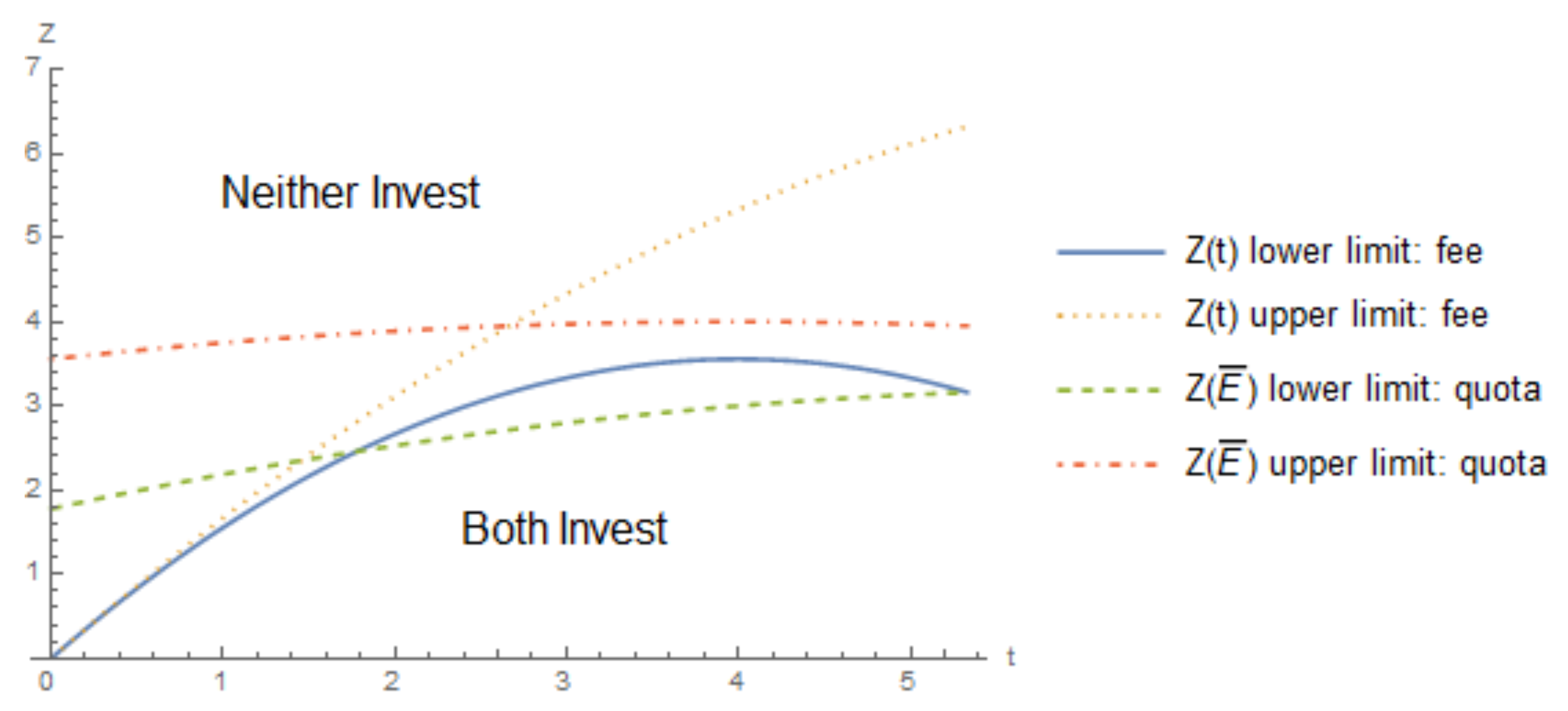
Similar to Figure 1, the regions of Z and $\overline{E}$ that support the three cases outlined in Proposition 2 are shown in Figure 2. The intuition in the case of the quota follows that of the fee. If the cost of adoption is too high, neither firm will invest in the green technology. If the quota is stringent (low), the adoption cost needs to be low in order for the firms to invest since the increase in market profits are small (not including the investment cost). If the quota is high, adoption does little to increase output, the change in profits is small, and there is little incentive to invest in the technology.

2.3. Comparison of the Fee and Quota

Next, I compare the incentives for firms to invest in the abatement technology under a fee and quota. To facilitate the comparison, I establish an equivalency between the fee and quota by setting the emissions resulting from under a fee to the emissions quota, which occurs at

$$\overline{E}\equiv q_k{e}_k=(\gamma -\alpha )\frac{1}{3}[a-c-(\gamma -\alpha )t].$$

This equivalency models the setting where an emission fee is set to meet a particular emissions target, which, in this case, is the quota. The following lemma summarizes the relationship between the thresholds that determine the Nash equilibria under the fee and quota, as described in Propositions 1 and 2.

Lemma 1.

If policy is set so that emissions under the fee and quota are equivalent, then the Nash equilibrium where both firms adopt the technology is sustained at higher levels of the adoption cost under a fee than under a quota if $t\in (\underline{t},\overline{t})$, where $\underline{t}=\frac{(a-c)\left({\gamma }^2-2{\alpha }^2+5\alpha \gamma \right)-\gamma \sqrt{{(a-c)}^2(\gamma -\alpha )(7\alpha +\gamma )}}{2\left({\alpha }^3-5{\alpha }^2\gamma +7\alpha {\gamma }^2+{\gamma }^3\right)}$ and $\overline{t}=\frac{(a-c)\left({\gamma }^2-2{\alpha }^2+5\alpha \gamma \right)+\gamma \sqrt{{(a-c)}^2(\gamma -\alpha )(7\alpha +\gamma )}}{2\left({\alpha }^3-5{\alpha }^2\gamma +7\alpha {\gamma }^2+{\gamma }^3\right)}$.

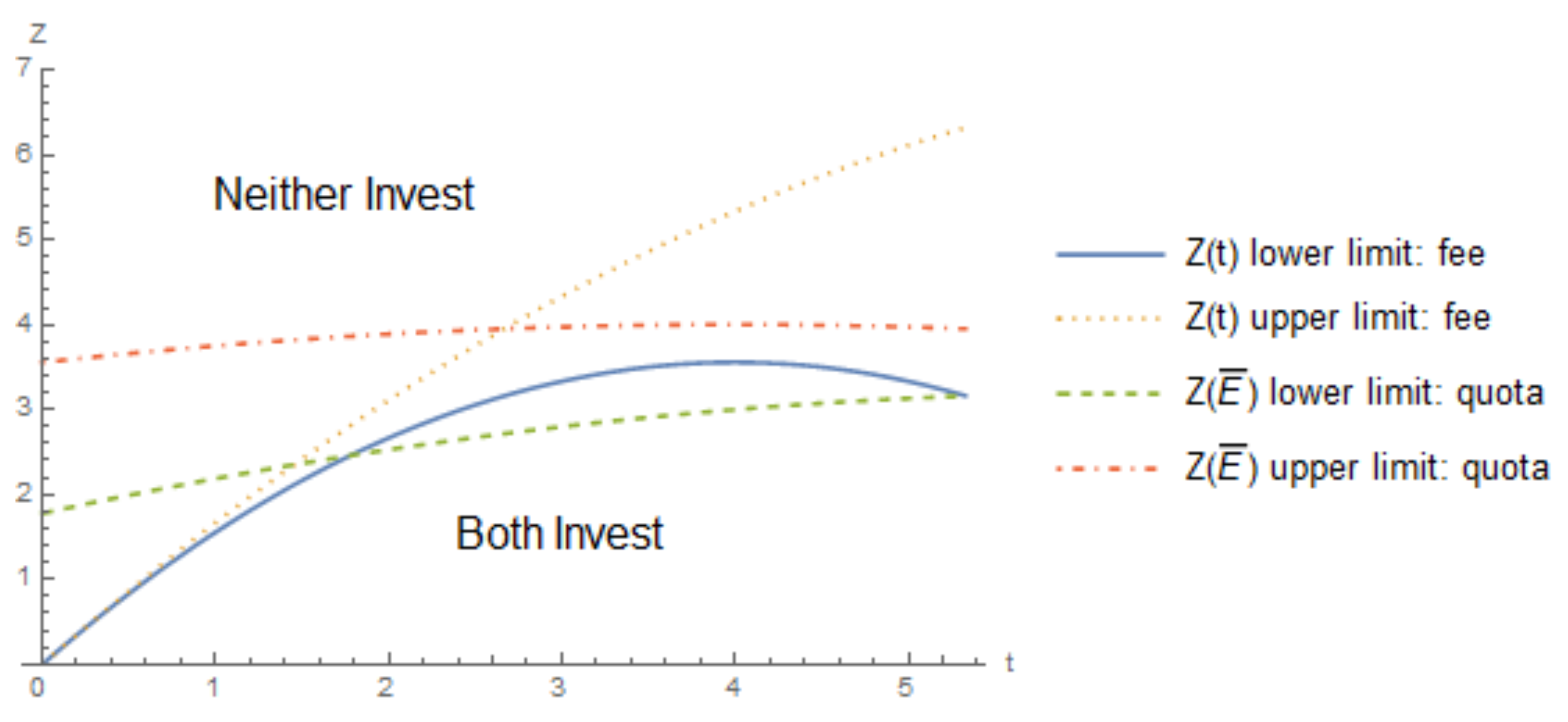
To aid in the intuition of this lemma, consider Figure 3, which overlays the limits from Figure 2 on Figure 1. Note that a lower fee corresponds to a less stringent quota.15 At less restrictive policy levels, firms are more willing to adopt a more expensive technology under a quota. However, this ranking reverses as policy becomes more stringent and firms are more willing to adopt an expensive technology under a fee than under a quota.

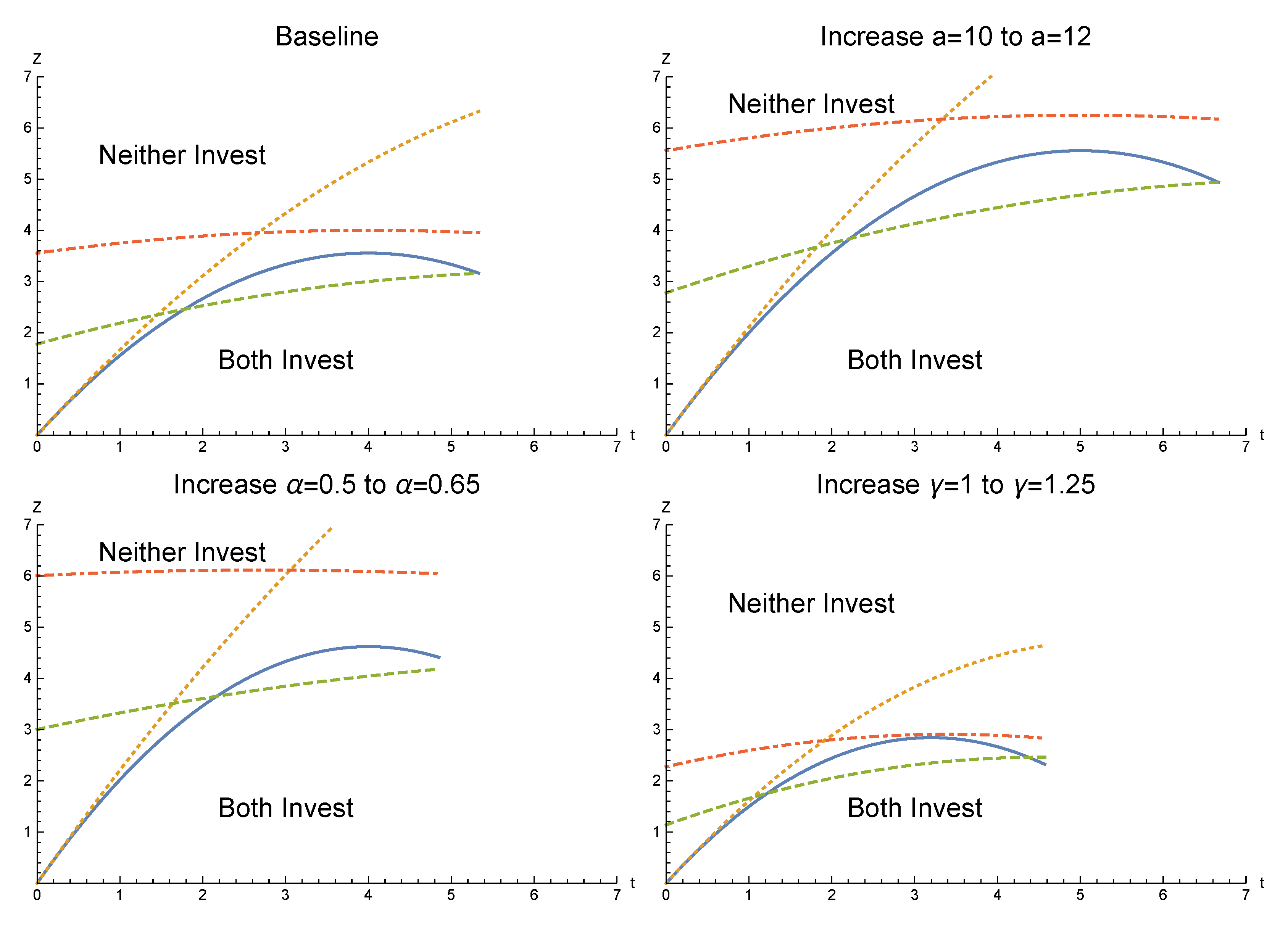
Then next step is to investigate how market conditions and the nature of the effectiveness of the technology impact these cutoff by investigating the comparative statics on $\underline{t}$ and $\overline{t}$ with respect to $(a-c)$, $\gamma$, and $\alpha$. These are summarized as follows and graphically aided by Figure 4:16

Market size:	${\displaystyle \frac{\partial \underline{t}}{\partial (a-c)}}>0$, and	${\displaystyle \frac{\partial \overline{t}}{\partial (a-c)}}>0$
Emissions:	${\displaystyle \frac{\partial \underline{t}}{\partial \gamma }}<0$, and	${\displaystyle \frac{\partial \overline{t}}{\partial \gamma }}>0$
Abatement:	${\displaystyle \frac{\partial \underline{t}}{\partial \alpha }}>0$, and	${\displaystyle \frac{\partial \overline{t}}{\partial \alpha }}<0$

A shift to the right of the lower crossing point $\underline{t}$, caused by an increase in the difference between maximum willingness to pay and marginal cost of production $(a-c)$, or a more effective abatement technology $\alpha$, increases the range where firms adopt a more expensive technology under a quota. An increase in $(a-c)$ increases profit under each policy; however, this increase is greater under the quota as an increase in $(a-c)$ necessitates an increase in the emission fee to keep emissions equivalent across the two policies. The larger increase in profit under the quota implies that the firm is more willing to invest in a more expensive abatement technology under the quota. Similarly, an increase in the effectiveness of the abatement technology $\alpha$ requires an increase in the fee to facilitate equivalent emissions under the two policies, thus decreasing the resulting profit under the fee when compared to that under a quota. An increase in the per unit emissions $\gamma$ decreases the lower range where the quota is more effective at encouraging adoption of expensive technology, following similar intuition to an decrease in $\alpha$.

At the high crossing point $\overline{t}$, an increase in the effectiveness of the abatement technology $\alpha$ (or decrease in emissions $\gamma$) has a similar impact as at the lower end as it increases the upper limit of the adoption cost where both of the firms adopt the technology more under the quota than the fee. Combining the effects, lower emissions (through either low-emitting production or more effective technology) reduces the range over which both firms adopt a more expensive technology under a fee than under a quota.

The combination of these results informs us of some intuitive results under each policy regime. That is, when demand is higher (higher a), the marginal cost is lower (c), or the abatement technology is more effective at reducing emissions, both firms are willing to adopt a more expensive technology. However, a more polluting production process results in firms being less willing to adopt a costly technology and the cost limit of the technology is reduced. Though these results are consistent across policy regimes, the changes to $\underline{t}$ and $\overline{t}$ show that the investment cost limits under a quota are more sensitive to changes in these parameters.

The next step is to evaluate the social welfare at the Nash equilibrium, where both firms invest in the green technology under each of the policy mechanisms. Social welfare is calculated as the sum of consumer and producer surplus and tax revenue (if applicable), net environmental damage, and green technology investment,17

$$SW={\int }_0^{Q_2}(a-c-x)dx-d{(e_{i2}+e_{j2})}^2-2Z.$$

This comparison is described in the following lemma.

Lemma 2.

If policy is set so that emissions under the fee and quota are equivalent and both firms adopt the technology, then social welfare under a fee is equivalent to social welfare under a quota.

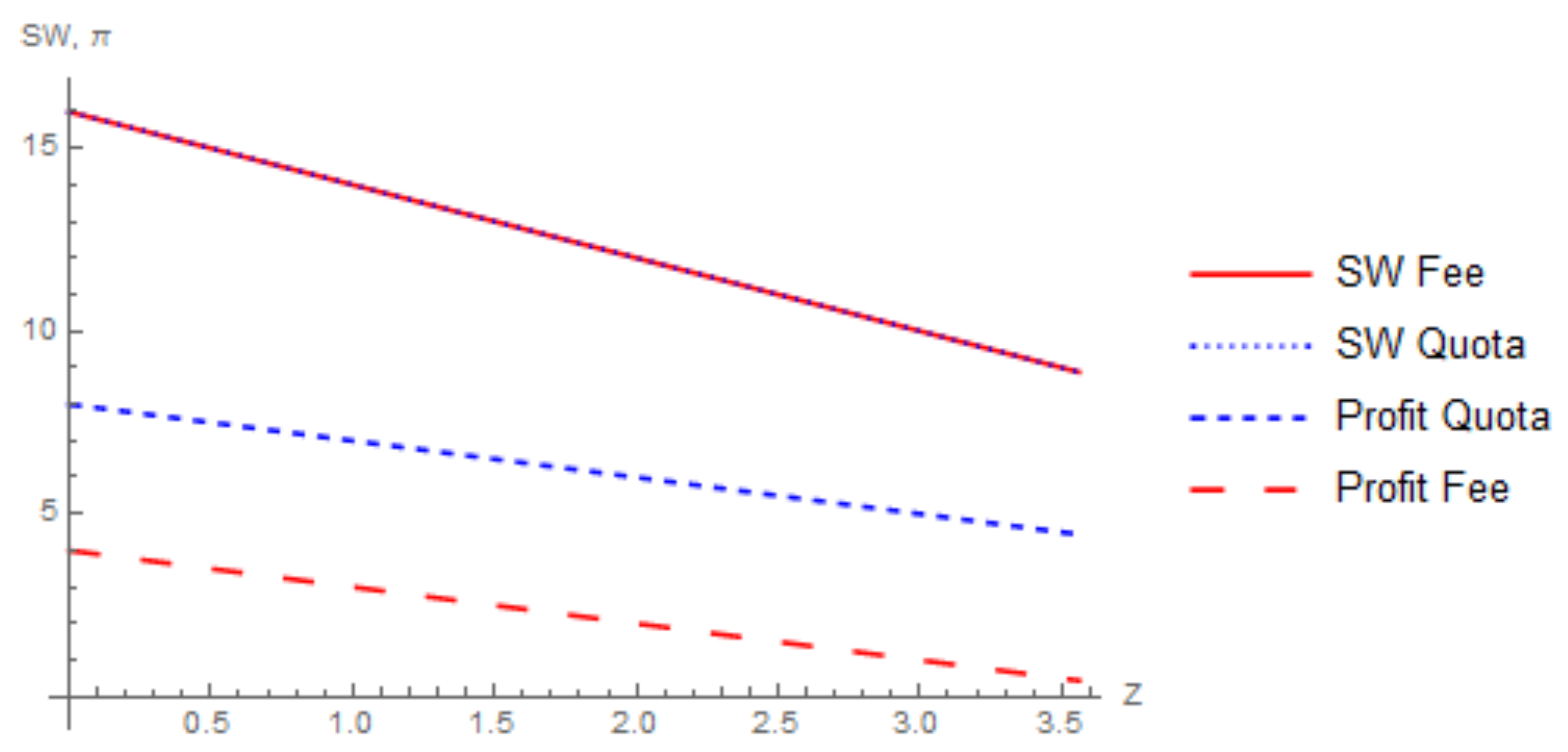
The policy equivalence leads to a situation where the only difference between the policy outcomes is the firms’ profits, which differs by the level of the emission fee. Figure 5 plots social welfare and individual firm profit under each policy.18 This analysis shows that although the regulator does not have a preferred policy, firms do. A similar conclusion is found in Wenders (1975), who showed that firms have little incentive to provide pollution abatement under an emission fee. Under a fee, firms face what is essentially an increase in the marginal cost of production, whereas, under a quota, firms only incur their original marginal cost, but are limited to a certain quantity, thus achieving a higher profit under the quota.

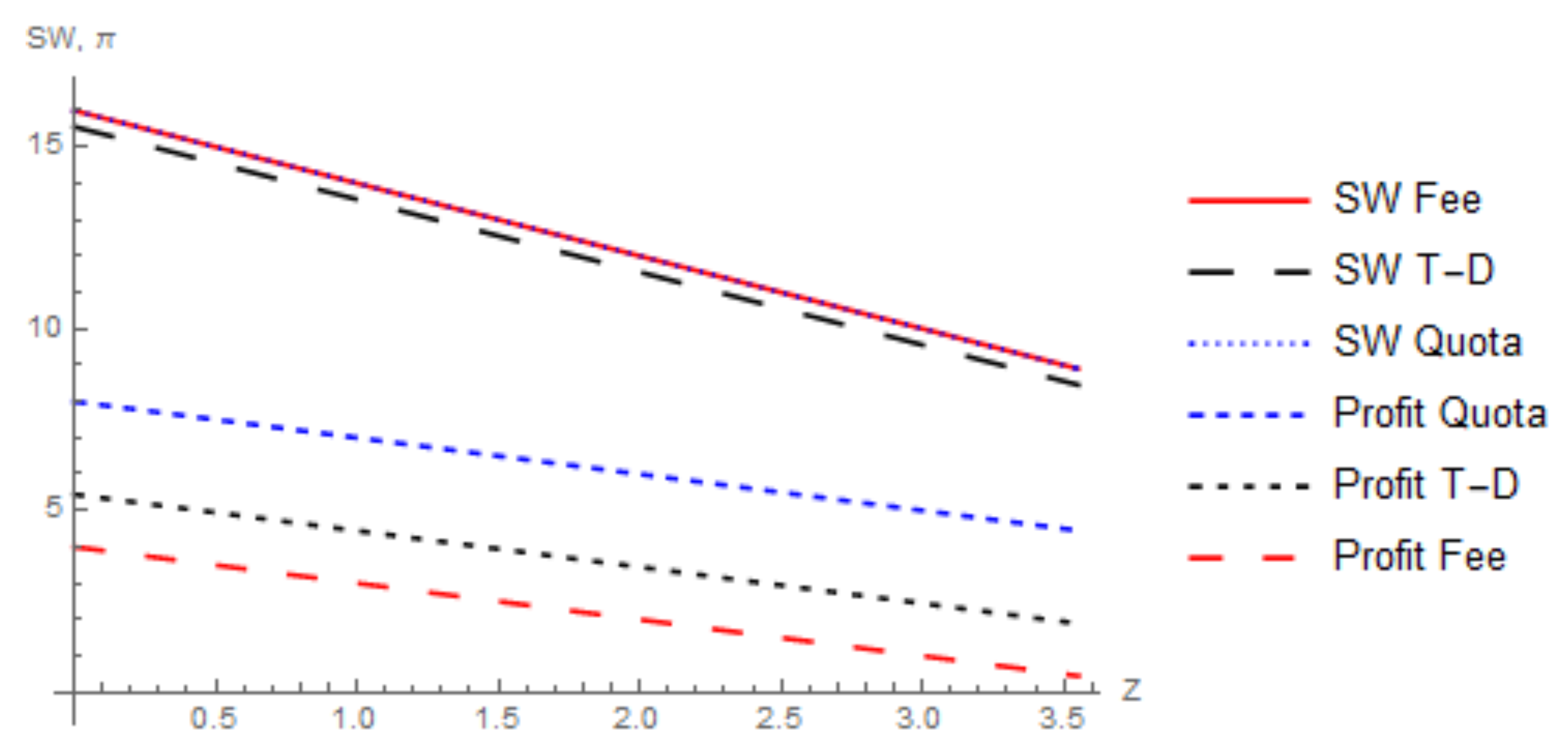
Figure 6 adds to Figure 5 by including social welfare and profits under the type-dependent fee (T-D), where there is a 50% reduction in the fee if the firms adopt the technology.19 The reduced fee increases production and emissions as compared to the baseline fee. This means that firm profits are increased and there is more environmental damage. The latter effect dominates the former and social welfare is reduced under the type-dependent fee. However, the incentive to adopt the technology increases and firms are willing to adopt the technology at a higher cost than without the fee reduction.

2.4. Asymmetric Cost of Adoption under an Emission Fee

The first asymmetry to explore is when firms have different costs of adoption, which is $Z_i\ne Z_j$. Without a loss of generality, I assume that firm i has a lower cost of technology adoption than firm j, so that $Z_i<Z_j$. The equilibrium is best explained while using best-response function,

$$\begin{array}{c}\hfill \mathrm{firm}i\mathrm{will}\left\{\begin{array}{cc}invest\mathrm{if}\hfill & \mathrm{firm}jinvestsand{Z}_i<\frac{1}{9}\left(4t\alpha (a-c-t\gamma )\right)\\ invest\mathrm{if}\hfill & \mathrm{firm}jdoesnotinvestand{Z}_i<\frac{1}{9}\left(4t\alpha (a-c-t(\gamma -\alpha ))\right)\\ notinvest\hfill & \mathrm{otherwise}\end{array}\right.\end{array}$$

Firm j has a symmetric best response function. This leads to the following corollary that summarizes the Nash equilibria.

Corollary 1.

In the case of asymmetric adoption costs, the equilibrium adoption decisions are:

1. 

Both of the firms adopt the technology if $Z_j<\frac{1}{9}\left(4t\alpha (a-c-t\gamma )\right)$.

2. 

Neither firm adopts the technology if $Z_i>\frac{1}{9}\left(4t\alpha (a-c-t(\gamma -\alpha ))\right)$.

3. 

Only one firm adopts the technology if $\frac{1}{9}\left(4t\alpha (a-c-t\gamma )\right)<Z_i<Z_j<\frac{1}{9}\left(4t\alpha (a-c-t(\gamma -\alpha ))\right)$.20

4. 

Only the low cost firm i adopts the technology if $Z_i<\frac{1}{9}\left(4t\alpha (a-c-t(\gamma -\alpha ))\right)<Z_j$.

The first three cases of this corollary are similar to the Proposition 1, where both firms invest if the adoption cost is low, neither invests if the cost is too high, and a third case where the Nash equilibrium is for only one firm to invest. In the third case, even though firm i has a lower adoption cost, a Nash equilibrium where only the high cost firm adopts exists. In this case, firm i’s best response to firm j’s adoption is to not adopt the technology (and firm j’s best response to firm i adopting is to not adopt). This case only happens when the cost of adoption to both of the firms is moderately high and the discrepancy between the adoption costs is small.

A fourth case exists where the Nash equilibrium is for only the low cost firm to invest in the green technology and the high cost firm to not invest in the technology, which happens if the adoption cost discrepancy is relatively large and the high cost firm faces a large adoption cost. In this case, the low cost firm gains a competitive advantage, since it can lower its emissions and pay a lower fee on each unit of production when compared to its rival.

2.5. Investment Increases Marginal Cost of Production under an Emission Fee

The second asymmetry to explore is where the adoption of the green technology increases the marginal cost of production from c to $c^{\prime }$.21 In addition to the fixed costs of adopting a green technology, the abatement process itself is costly on a per-unit basis, thus the marginal cost of producing each unit increases. For instance, this can happen if the technology requires maintenance or if the the adopted technology needs additional labor in order to abate the emissions.22 In this setting, profits in the first stage are unaffected, but second stage profits if the firm invests are

$${\Pi }_i^{INV}=(a-(q_{i2}+q_{j2}))q_{i2}-c^{\prime }{q}_{i2}-t(\gamma -\alpha )q_{i2}.$$

In this setting, there are three potential equilibria, which are presented in the following proposition.

Proposition 3.

In the case where adoption increases the marginal cost of production under an emission fee, the equilibrium adoption decisions are:

1. 

Both of the firms adopt the technology if $Z<\frac{4}{9}(a-c-t\gamma )(t\alpha +c-c^{\prime })$.

2. 

Neither firm adopts the technology if $Z>\frac{4}{9}(t\alpha +c-c^{\prime })(a-c^{\prime }-t(\gamma -\alpha ))$.

3. 

Only one firm adopts the technology if $\frac{4}{9}(t\alpha +c-c^{\prime })(a-c-t\gamma )<Z<\frac{4}{9}(t\alpha +c-c^{\prime })(a-c^{\prime }-$$t(\gamma -\alpha ))$.23

The intuition for each of the equilibria is similar to that of Proposition 1, with the addition of the conditions on the increase in marginal cost. That is, if adoption of the technology is costly ($Z>0$), then, for both firms to adopt the technology, it must be that $t\alpha +c-c^{\prime }>0$, or,

$$c^{\prime }-c<t\alpha .$$

This means that, if firms adopt the technology, it must be that the decrease in the emission fee per unit produced outweighs the increase in marginal cost of production. A larger increase in the marginal cost of production requires a lower adoption cost if both (or one) of the firms to adopt the technology.

2.6. Type-Dependent Fee

Next, I investigate the case where a firm faces a lower emission fee if they adopt a the green technology. Specifically, the fee will decrease from t to $t^{\prime }$.24 This case represents the situation where the regulator can adjust its policy if a firm adopts and uses a green technology (e.g., CO${}_2$ scrubbers) and “rewards” the firm by imposing a lower fee on its emissions. This setting does not affect the first stage, but it does impact second-stage profits if the firm adopts, such that

$${\Pi }_i^{INV}=(a-(q_{i2}+q_{j2}))q_{i2}-c{q}_{i2}-t^{\prime }(\gamma -\alpha )q_{i2}.$$

In this case, firm i’s reaction function is

$$\begin{array}{c}\hfill \mathrm{firm}i\mathrm{will}\left\{\begin{array}{cc}invest\mathrm{if}\hfill & \mathrm{firm}jinvestsandZ<\frac{4}{9}(a-c-t\gamma )(t\gamma -t^{\prime }(\gamma -\alpha ))\\ invest\mathrm{if}\hfill & \mathrm{firm}jdoesnotinvestandZ<\frac{4}{9}(a-c-t^{\prime }(\gamma -\alpha ))(t\gamma -t^{\prime }(\gamma -\alpha ))\\ notinvest\hfill & \mathrm{otherwise}\end{array}\right.\end{array}$$

The Nash equilibria are presented in the following proposition.

Proposition 4.

In the case of a type-dependent fee, the equilibrium adoption decisions are:

1. 

Both firms adopt the technology if $Z<\frac{4}{9}(a-c-t\gamma )(t\gamma -t^{\prime }(\gamma -\alpha ))$.

2. 

Neither firm adopts the technology if $Z>\frac{4}{9}(a-c-t^{\prime }(\gamma -\alpha ))(t\gamma -t^{\prime }(\gamma -\alpha ))$.

3. 

Only one firm adopts the technology if $\frac{4}{9}(a-c-t\gamma )(t\gamma -t^{\prime }(\gamma -\alpha ))<Z<\frac{4}{9}(a-c-t^{\prime }(\gamma -\alpha ))(t\gamma -t^{\prime }(\gamma -\alpha ))$.25

This proposition follows the same basic intuition of the previous case, except that the limits on the investment are now affected by the new, lower emission fee in each case of adoption. Because adoption decreases both the emissions and emission fee, firms see a larger benefit to adoption than under the uniform fee. This means that firms are more willing to adopt a more expensive technology, as seen in the next section.

2.7. Comparison of Investment Limits under a Fee

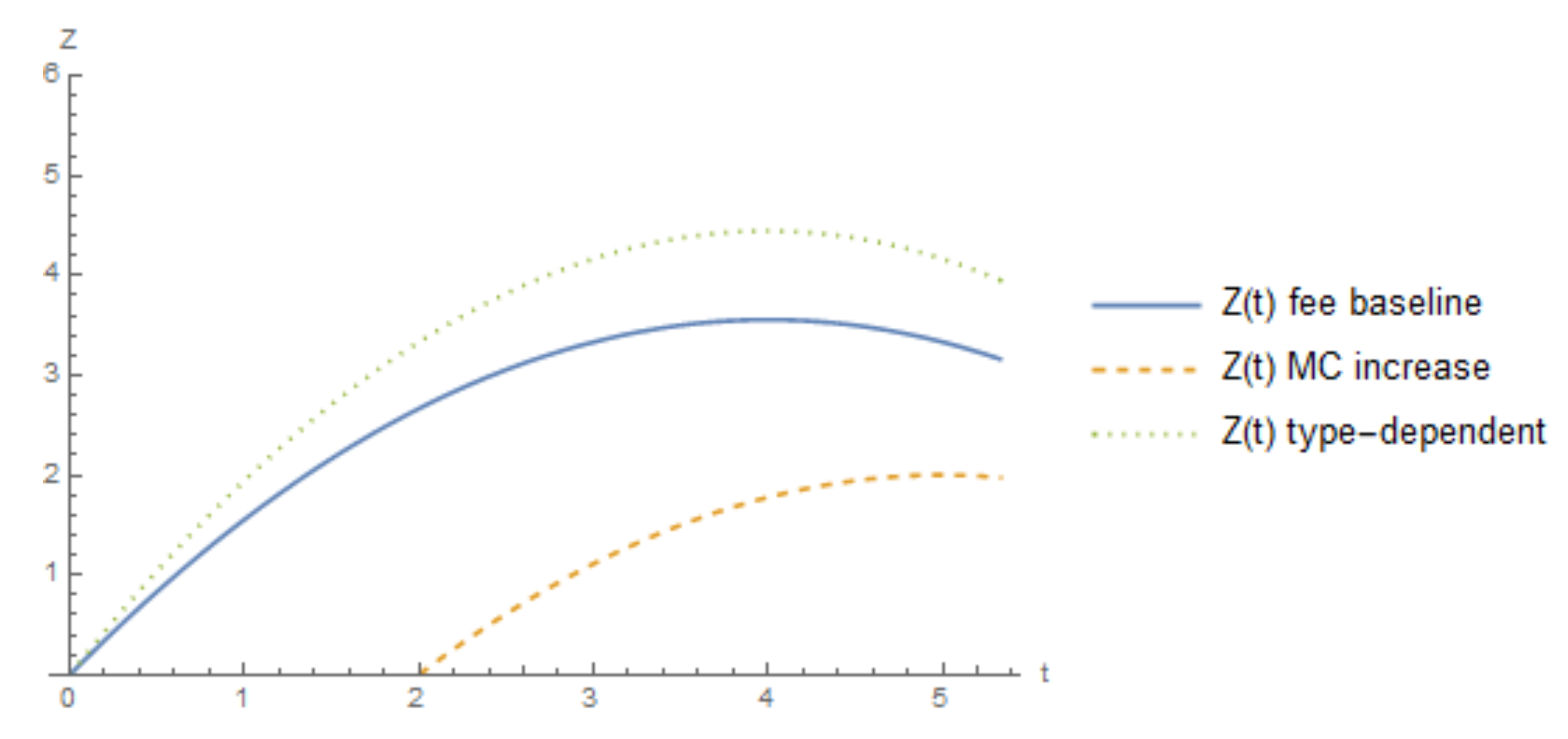
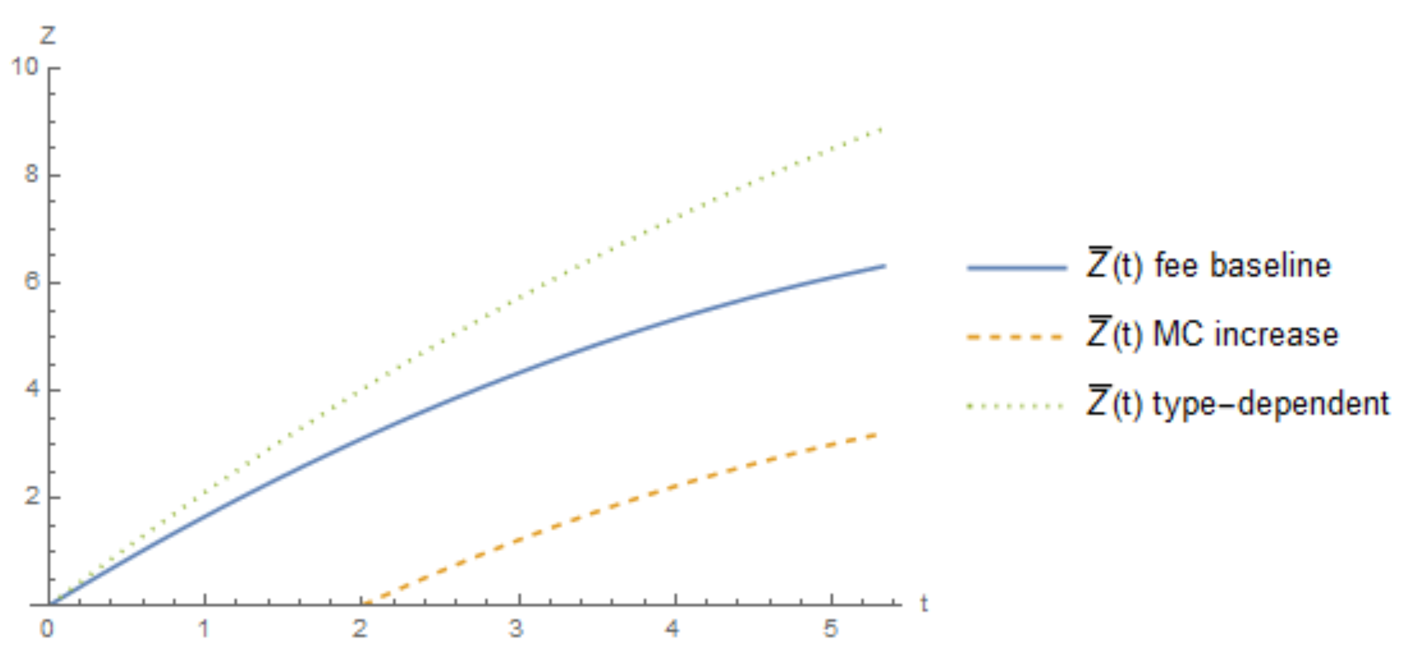
At this point, it is worth comparing the different limits on the investment cost, which supports an equilibrium where both firms invest between the three cases presented thus far: baseline (symmetric), investment increases marginal cost, and the type-dependent fee. The levels of Z and t where both firms adopt the technology is the region under their respective line presented for each case in Figure 7.26 This figure shows that under the type-dependent fee, the upper limit on investment cost is higher than either the baseline or marginal cost increase case. This is a direct result of the increased benefit from facing a lower fee from adoption as compared to the other cases. When the investment increases the marginal cost the limit on the investment cost is most restrictive. Figure 8 shows the lower limit of investment cost that supports the equilibrium, where neither firm adopts the technology. A similar ranking occurs as with the limit on cost that supports both firms adopting (Figure 7).

Because the cutoff on the level of investment that facilitates both firms investing is lower when the green technology increases marginal cost and the type-dependent fee increases the level of investment limit, a potential policy option is for the regulator to implement a type-dependent fee if the cost of investment increases the marginal cost. The type-dependent fee has the effect of reducing the marginal cost, so that the regulator compensates the firm for any increase in marginal cost from adopting the technology through a lower fee. This could be set, so that the fee reduction perfectly corrects for the increase in marginal cost or over-corrects for the increase and rewards the firm for the investment by having a lower overall marginal cost for the adoption.

2.8. Tradeable Permit Scheme

In a tradeable permit scheme (cap-and-trade), the regulator sets an emissions cap for all firms in the economy and distributes permits (either through appropriation or auction), and firms can buy and sell permits as needed. If the market for permits is perfectly competitive, then the price on permits acts the same as an emission fee if all of the firms are price takers in the permit market. This leads to the same equilibrium as in Proposition 1, where t is the permit price. Hence, the analysis for a tradeable permit scheme is identical to the emission fee for all of the extensions.

2.9. Asymmetric Cost of Adoption under a Quota

The following corollary summarizes the equilibria that can occur if the firms have asymmetric costs of adopting the green technology, where firm j has the higher adoption cost. The equilibrium quantities and profits are the same as under the baseline quota, only that $Z_i<Z_j$.

Corollary 2.

In the case of a quota where firms have asymmetric costs of adoption, the equilibrium adoption decisions are:

1. 

Both of the firms adopt the technology if $Z_i<Z_j<\frac{\overline{E}\alpha (\gamma (a-c)(\gamma -\alpha )-\overline{E}(3\gamma -\alpha ))}{{(\gamma -\alpha )}^2{\gamma }^2}$.

2. 

Neither firm adopts the technology if $Z_j>Z_i>\frac{\overline{E}\alpha (\gamma (a-c)(\gamma -\alpha )-\overline{E}(3\gamma -2\alpha ))}{{(\gamma -\alpha )}^2{\gamma }^2}$.

3. 

Only one firm adopts the technology if

$\frac{\overline{E}\alpha (\gamma (a-c)(\gamma -\alpha )-\overline{E}(3\gamma -\alpha ))}{{(\gamma -\alpha )}^2{\gamma }^2}<Z_i<Z_j<\frac{\overline{E}\alpha (\gamma (a-c)(\gamma -\alpha )-\overline{E}(3\gamma -2\alpha ))}{{(\gamma -\alpha )}^2{\gamma }^2}$.27

4. 

Only the low cost firm i adopts the technology if $Z_i<\frac{\overline{E}\alpha (\gamma (a-c)(\gamma -\alpha )-\overline{E}(3\gamma -\alpha ))}{{(\gamma -\alpha )}^2{\gamma }^2}<Z_j$.

Similar to under the fee when adoption costs are asymmetric, the low cost adopter is more willing to adopt the technology although both of the firms will adopt if the technology is cheap enough. It is also possible that the high cost firm can adopt and the low cost firm will not adopt if the technology cost for both firms is relatively high, as each of their best-responses is to do the opposite of the other firm.

2.10. Investment Increases Marginal Cost of Production under a Quota

The case when investment in the green technology increases the marginal cost of production from c to $c^{\prime }$ under a quota is presented in the following proposition. In this setting, equilibrium quantities are the same under a quota, since the quota is binding, but the profit if the firm invests in the technology is ${\Pi }_{i2}^{INV}=(a-(q_{i2}+q_{j2}))q_{i2}-c^{\prime }{q}_{i2}$.

Proposition 5.

In the case of a quota where adoption increases the firm’s marginal cost of production, the equilibrium adoption decisions are:

1. 

Both firms adopt the technology if $Z<\frac{\overline{E}(\alpha \overline{E}(\alpha -3\gamma )-\gamma (\alpha -\gamma )((a-c)\alpha +(c-c^{\prime })\gamma ))}{{\gamma }^2{(\alpha -\gamma )}^2}$, and $c^{\prime }-c<\frac{(a-c)\alpha }{\gamma }$.

2. 

Neither firm adopts the technology if $Z>\frac{\overline{E}(\alpha \overline{E}(2\alpha -3\gamma )-\gamma (\alpha -\gamma )((a-c)\alpha +(c-c^{\prime })\gamma ))}{{\gamma }^2{(\alpha -\gamma )}^2}$

3. 

Only one firm adopts the technology if

$\frac{\overline{E}(\alpha \overline{E}(\alpha -3\gamma )-\gamma (\alpha -\gamma )((a-c)\alpha +(c-c^{\prime })\gamma ))}{{\gamma }^2{(\alpha -\gamma )}^2}<Z<\frac{\overline{E}(\alpha \overline{E}(2\alpha -3\gamma )-\gamma (\alpha -\gamma )((a-c)\alpha +(c-c^{\prime })\gamma ))}{{\gamma }^2{(\alpha -\gamma )}^2}$, and $c^{\prime }-c<\frac{(a-c)\alpha }{\gamma }$.28

The intuition for this set of equilibria align with that in the case of an emission fee where the adoption of the technology increases marginal costs, and it has the same limits on the increase in costs that causes the firms to not invest in the technology. If the costs of adoption are low, both of the firms will invest. If the cost of adoption is too high, then neither firm will invest in the technology. This equilibrium can also happen if the increase in marginal cost is too high, i.e., $(c^{\prime }-c)>\frac{(a-c)\alpha }{\gamma }$. There is also a region of costs between these two equilibria where the equilibrium is for one firm to adopt and a mixed strategy can exist.

3. Discussion

The consensus in the literature is that market-based policies, such as fees, outperform command-and-control policies when evaluated on the basis of social costs (adoption cost and environmental damage). The game-theoretic approach taken here finds that regulators are indifferent between employing a fee or a quota in terms of achieving the highest social welfare. However, firms enjoy higher profits under a quota than under an equivalent fee. In addition, the equilibrium resulting in both firms adopting the technology is sustained at higher levels of adoption cost under a fee than under a quota when the policies are not very stringent. However, this result is reversed for moderately stringent levels of policy. Given a promising underused technology in an industry facing a less restrictive policy, it may be in the regulator’s best interest to either employ a more restrictive quota or a relatively lax fee for the purpose of encouraging adoption of the technology and reducing emissions, especially in the case of relatively expensive technology. If an emission fee is currently being used, to encourage adoption the regulator might consider two options: (1) increasing the fee in order to encourage adoption to mitigate the costs of regulation, (2) employing a more restrictive quota, or (3) subsidizing the technology adoption.

Another policy option is that of the type-dependent fee where the firm faces a lower emission fee if it chooses to adopt the technology. This policy option lowers social welfare slightly, because it results in higher emissions, but increases firm profits closer to the profit achieved under the quota. Combining the type-dependent fee with an adoption subsidy has the best chance of aligning firm and regulator incentives.

This analysis could be furthered by exploring the what happens when firms have production functions with asymmetric emissions. Each firm has more incentive to invest as the more efficient firm could increase its cost advantage by investing in the technology and the less efficient firms becomes more competitive if it invests in the technology. Another possible extension is of asymmetric information where the firms are unaware of the emissions or costs of their competitor. Finally, allowing for the potential of consumer willingness to pay to increase when the firm invests the green technology would increase the benefits from adoption further than simply lower emissions.

4. Materials and Methods

4.1. Outline of Proof of Proposition 1

In the case that neither firm invests, the equilibrium is solved by the following system of best response function from Section 2.1, which is,

$$\begin{array}{cc}\hfill q_i& ={\displaystyle \frac{a-c-t\gamma }{2}}-{\displaystyle \frac{1}{2}}{q}_j,\mathrm{and}{q}_j={\displaystyle \frac{a-c-t\gamma }{2}}-{\displaystyle \frac{1}{2}}{q}_i.\hfill \end{array}$$

Solving this system yields the symmetric equilibrium outputs of $q_i=q_j=\frac{1}{3}(a-c-\gamma t)$, with resulting profit ${\Pi }_i^{NI,NI}=\frac{1}{9}{(a-c-t\gamma )}^2$.

If both firms invest, equilibrium quantities are found by solving the following system of best response functions,

$$\begin{array}{cc}\hfill q_i& ={\displaystyle \frac{a-c-t(\gamma -\alpha )}{2}}-{\displaystyle \frac{1}{2}}{q}_j,\mathrm{and}{q}_j={\displaystyle \frac{a-c-t(\gamma -\alpha )}{2}}-{\displaystyle \frac{1}{2}}{q}_i.\hfill \end{array}$$

Solving for quantities gives the equilibrium when both firms invest of $q_i=q_j=\frac{1}{3}(a-c-t(\gamma -\alpha ))$, and profits of ${\Pi }_i^{INV,INV}=\frac{1}{9}{(a-c-t(\gamma -\alpha ))}^2$.

If firm i invests and firm j does not invest, the following system is used

$$\begin{array}{cc}\hfill q_i& ={\displaystyle \frac{a-c-t(\gamma -\alpha )}{2}}-{\displaystyle \frac{1}{2}}{q}_j,\mathrm{and}{q}_j={\displaystyle \frac{a-c-t\gamma }{2}}-{\displaystyle \frac{1}{2}}{q}_i.\hfill \end{array}$$

The equilibrium quantities are $q_i=\frac{1}{3}(a-c-t(\gamma -2\alpha ))$ and $q_j=\frac{1}{3}(a-c-t(\gamma +\alpha ))$. Plugging these quantities into their respective firm’s profit function yields ${\Pi }_i^{INV,NI}=\frac{1}{9}{(a-c-t(\gamma -2\alpha ))}^2$ and ${\Pi }_j^{NI,INV}=\frac{1}{9}{(a-c-t(\gamma +\alpha ))}^2$. Table 1 summarizes these.

If the dominant strategy for both firms is to invest, then the Nash equilibrium is (Invest, Invest). For this, both ${\Pi }_k^{INV,INV}-Z>{\Pi }_k^{NI,INV}$ and ${\Pi }_k^{INV,NI}-Z>{\Pi }_k^{NI,NI}$. More explicitly,

$$\begin{array}{cc}\hfill \frac{1}{9}{(a-c-t(\gamma -\alpha ))}^2-Z& >\frac{1}{9}{(a-c-t(\gamma +\alpha ))}^2,\mathrm{and}\hfill \\ \hfill \frac{1}{9}{(a-c-t(\gamma -2\alpha ))}^2-Z& >\frac{1}{9}{(a-c-t\gamma )}^2,\hfill \end{array}$$

which simplifies to

$$\begin{array}{cc}\hfill \frac{1}{9}\left(4\alpha t(a-c-t\gamma )\right)& >Z,\mathrm{and}\hfill \\ \hfill \frac{1}{9}\left(4\alpha t(a-c-t(\gamma -\alpha ))\right)& >Z.\hfill \end{array}$$

Because $Z<\frac{1}{9}\left(4\alpha t(a-c-t\gamma )\right)$ is more restrictive than the second inequality, this inequality is necessary and sufficient for (Invest, Invest) to be the Nash equilibrium.

The Nash equilibrium is (No Invest, No Invest) if both ${\Pi }_k^{NI,INV}>{\Pi }_k^{INV,INV}-Z$ and ${\Pi }_k^{NI,NI}>{\Pi }_k^{INV,NI}-Z$ hold, which simplifies to

$$\begin{array}{cc}\hfill \frac{1}{9}\left(4\alpha t(a-c-t\gamma )\right)& <Z,\mathrm{and}\hfill \\ \hfill \frac{1}{9}\left(4\alpha t(a-c-t(\gamma -\alpha ))\right)& <Z.\hfill \end{array}$$

For the (No Invest, No Invest) equilibrium, the more restrictive condition is needed, i.e., $Z>\frac{1}{9}\left(4\alpha t(a-c-t(\gamma -\alpha ))\right)$.

The final set of equilibria occurs when each firm will invest only if the other firm chooses not to invest, so the Nash equilibria are (Invest, No Invest), (No Invest, Invest) and a mixed strategy where firms will randomize over the two actions if the expected profit from investing and not investing are equal. This occurs when ${\Pi }_{k2}^{NI,INV}>{\Pi }_{k2}^{INV,INV}-Z$ and ${\Pi }_{k2}^{INV,NI}-Z>{\Pi }_{k2}^{NI,NI}$, which simplifies to

$$\begin{array}{cc}\hfill \frac{1}{9}\left(4\alpha t(a-c-t\gamma )\right)& <Z,\mathrm{and}\hfill \\ \hfill \frac{1}{9}\left(4\alpha t(a-c-t(\gamma -\alpha ))\right)& >Z.\hfill \end{array}$$

This is the range that Z needs to be in to support the (Invest, No Invest), (No Invest, Invest) equilibrium. If Z is in this range, and the probability of firm j adopting is ${\sigma }_t$, and not adopting is $1-{\sigma }_t$, then firm i is indifferent between adopting and not adopting if

$$\begin{array}{cc}\hfill {\sigma }_t({\Pi }_i^{INV,INV}-Z)+(1-{\sigma }_t)({\Pi }_i^{INV,NI}-Z)& ={\sigma }_t{\Pi }_i^{NI,INV}+(1-{\sigma }_t){\Pi }_i^{NI,NI},\hfill \\ \hfill {\sigma }_t(\frac{1}{9}{(a-c-t(\gamma -\alpha ))}^2-Z)+(1-{\sigma }_t)\left(\frac{1}{9}\right(a-c-& {t(\gamma -2\alpha ))}^2-Z)=\hfill \\ \hfill {\sigma }_t\left(\frac{1}{9}\right(a-c-& {t(\gamma +\alpha ))}^2)+(1-{\sigma }_t)\left(\frac{1}{9}{(a-c-t\gamma )}^2\right),\hfill \\ \hfill {\sigma }_t(4\alpha t(a-c-\gamma t)-9Z)& =(1-{\sigma }_t)(4\alpha t(a-c-t(\gamma -\alpha ))-9Z),\hfill \\ \hfill {\sigma }_t(4\alpha t(a-c-\gamma t)-4\alpha t(a-c-t(\gamma -\alpha )))& =4\alpha t(a-c-t(\gamma -\alpha \left)\right)-9Z,\hfill \\ \hfill {\sigma }_t& =\frac{4t\alpha (a-c-t(\gamma -\alpha \left)\right)-9Z}{4t^2{\alpha }^2}.\hfill \end{array}$$

A similar strategy is employed for the remaining propositions. The profits for each extension are given below.

4.2. Quota

In the case of a binding emissions quota, $\overline{E}=q_k{e}_k$, each firm k will choose $q_k=\frac{\overline{E}}{\gamma }$ if the firm does not invest in the abatement technology, and $q_k=\frac{\overline{E}}{\gamma -\alpha }$ if it does invest in the abatement technology. Profit functions from before are unchanged except that the firms no longer face a fee, which is,

$$\begin{array}{cc}\hfill {\Pi }_i^{INV}& =(a-(q_i+q_j))q_i-c{q}_i,\mathrm{and}\hfill \\ \hfill {\Pi }_i^{NI}& =(a-(q_i+q_j))q_i-c{q}_i.\hfill \end{array}$$

Plugging the appropriate equilibrium quantities into the above profit functions yields the equilibrium under each combination of invest and not invest, which are presented in

Table 3. Equilibrium quantity and profit under the baseline quota.

	Quantity	Profit
Neither firm invests	$q_i=\frac{\overline{E}}{\gamma }$	${\Pi }_i^{NI,NI}=\frac{\overline{E}(\gamma (a-c)-2\overline{E})}{{\gamma }^2}$
Both firms invest	$q_i=\frac{\overline{E}}{\gamma -\alpha }$	${\Pi }_i^{INV,INV}=\frac{\overline{E}((a-c)(\gamma -\alpha )-2\overline{E})}{{(\alpha -\gamma )}^2}$
Firm i invests, firm j does not	$q_i=\frac{\overline{E}}{\gamma -\alpha }$	${\Pi }_i^{INV,NI}=\frac{\overline{E}(\gamma (a-c)(\gamma -\alpha )-\overline{E}(2\gamma -\alpha ))}{\gamma {(\gamma -\alpha )}^2}$
Firm j invests, firm i does not	$q_i=\frac{\overline{E}}{\gamma }$	${\Pi }_i^{NI,NV}=\frac{\overline{E}\left(a-c-\overline{E}\left(\frac{1}{\gamma -\alpha }+\frac{1}{\gamma }\right)\right)}{\gamma }$

.

The limit on Z that supports the different equilibria is solved using the same process as Proposition 1. The Nash equilibrium is (Invest, Invest) if the dominant strategy for both firms is to invest. For this, both ${\Pi }_k^{INV,INV}-Z>{\Pi }_k^{NI,INV}$ and ${\Pi }_k^{INV,NI}-Z>{\Pi }_k^{NI,NI}$, which simplifies to

$$\begin{array}{cc}\hfill \frac{\overline{E}\alpha (\gamma (a-c)(\gamma -\alpha )-\overline{E}(3\gamma -\alpha ))}{{\gamma }^2{(\alpha -\gamma )}^2}& >Z,\mathrm{and}\hfill \\ \hfill \frac{\overline{E}\alpha (\gamma (a-c)(\gamma -\alpha )-\overline{E}(3\gamma -2\alpha ))}{{\gamma }^2{(\alpha -\gamma )}^2}& >Z.\hfill \end{array}$$

Because $Z<\frac{\overline{E}\alpha (\gamma (a-c)(\gamma -\alpha )-\overline{E}(3\gamma -\alpha ))}{{\gamma }^2{(\alpha -\gamma )}^2}$ is more restrictive than the second inequality, this is necessary and sufficient for (Invest, Invest) to be the Nash equilibrium. For this equilibrium to be feasible, the numerator must be positive, which is $\overline{E}<\frac{\gamma (a-c)(\gamma -\alpha )}{3\gamma -\alpha }$. This condition always holds, since for the quota to be binding it must be that the quantity under a quota, $q=\frac{\overline{E}}{\gamma -\alpha }$, is less than the profit maximizing quantity under no policy, which is $q=\frac{1}{3}(a-c)$ (found by plugging $t=0$ into the appropriate quantity found in Section 4.1), or,

$$\frac{\overline{E}}{\gamma -\alpha }<\frac{1}{3}(a-c).$$

Solving for $\overline{E}$ yields $\overline{E}<\frac{1}{3}(a-c)(\gamma -\alpha )$. The numerator is always positive if $\overline{E}<\frac{1}{3}(a-c)(\gamma -\alpha )<\frac{\gamma (a-c)(\gamma -\alpha )}{3\gamma -\alpha }$. The second inequality simplifies to $\frac{1}{3}<\frac{\gamma }{3\gamma -\alpha }$, which always holds by assumption. The other equilibria are found by changing the inequalities above.

Next, I investigate whether the adopting firm’s output is bound by the quota in the case that only one firm adopts. If firm i adopts the technology and firm j does not, firm i’s best response function is $q_i=\frac{1}{2}(a-c)-\frac{1}{2}{q}_j$. Firm j’s equilibrium quantity, bound by the quota, is $q_j=\overline{E}/\gamma$. Plugging this into firm i’s best response function yields

$$q_i=\frac{a-c}{2}-\frac{1}{2}\frac{\overline{E}}{\gamma }.$$

The quota is binding if this quantity is greater than the quantity produced at the emissions quota, $\overline{E}/(\gamma -\alpha )$, or

$$\frac{a-c}{2}-\frac{1}{2}\frac{\overline{E}}{\gamma }>\frac{\overline{E}}{\gamma -\alpha }.$$

Rearranging, we have that

$$a-c>\frac{2\overline{E}}{\gamma -\alpha }+\frac{\overline{E}}{\gamma }.$$

By assumption, $\overline{E}<\frac{1}{3}(a-c)(\gamma -\alpha )$, and the right-hand side of the above inequality satisfies

$$\frac{2}{\gamma -\alpha }\left(\frac{1}{3}(a-c)(\gamma -\alpha )\right)+\frac{1}{\gamma }\left(\frac{1}{3}(a-c)(\gamma -\alpha )\right)\ge \frac{2\overline{E}}{\gamma -\alpha }+\frac{\overline{E}}{\gamma }.$$

Accordingly, it is sufficient to show that, if

$$a-c>\frac{2}{\gamma -\alpha }\left(\frac{1}{3}(a-c)(\gamma -\alpha )\right)+\frac{1}{\gamma }\left(\frac{1}{3}(a-c)(\gamma -\alpha )\right),$$

then the quota is binding for the adopting firm. The inequality first reduces to

$$1>\frac{2}{3}+\frac{1}{3\gamma }(\gamma -\alpha ),$$

and finally to

$$1>\frac{\gamma -\alpha }{\gamma },$$

which holds by assumption and, hence, the quota is also binding for the investing firm.

A similar proof also shows that if the quota is binding for the investing firm, then is must be binding for the non-investing firm. If firm i adopts the technology and firm j does not, firm j’s best response function is $q_j=\frac{1}{2}(a-c)-\frac{1}{2}{q}_i$. Firm i’s equilibrium quantity, bound by the quota, is $q_j=\overline{E}/(\gamma -\alpha )$. Plugging this into firm j’s best response function yields

$$q_j=\frac{a-c}{2}-\frac{1}{2}\frac{\overline{E}}{\gamma -\alpha }.$$

The quota is binding if this quantity is greater than the quantity produced at the emissions quota, $\overline{E}/\gamma$, or

$$\frac{a-c}{2}-\frac{1}{2}\frac{\overline{E}}{\gamma }>\frac{\overline{E}}{\gamma }.$$

Rearranging, we have that

$$a-c>\frac{\overline{E}}{\gamma -\alpha }+\frac{2\overline{E}}{\gamma }.$$

By assumption, $\overline{E}<\frac{1}{3}(a-c)(\gamma -\alpha )$, and the right-hand side of the above inequality satisfies

$$\frac{1}{\gamma -\alpha }\left(\frac{1}{3}(a-c)(\gamma -\alpha )\right)+\frac{2}{\gamma }\left(\frac{1}{3}(a-c)(\gamma -\alpha )\right)\ge \frac{\overline{E}}{\gamma -\alpha }+\frac{2\overline{E}}{\gamma }.$$

Hence, it is sufficient to show that if

$$a-c>\frac{1}{\gamma -\alpha }\left(\frac{1}{3}(a-c)(\gamma -\alpha )\right)+\frac{2}{\gamma }\left(\frac{1}{3}(a-c)(\gamma -\alpha )\right),$$

then the quota is binding for the non-adopting firm. The inequality first reduces to

$$1>\frac{1}{3}+\frac{2(\gamma -\alpha )}{3\gamma },$$

and, finally, to

$$1>\frac{3\gamma -2\alpha }{3\gamma },$$

which holds by assumption, and hence, the quota is also binding for the non-investing firm.

If a mixed strategy exists (where only one firm adopts the technology) and the probability that firm j adopts the technology is ${\sigma }_Q$ and the probability firm j does not invest is $(1-{\sigma }_Q)$, then firm i is indifferent between invest and no invest if

$$\begin{array}{cc}\hfill {\sigma }_Q({\Pi }_{i2}^{INV,INV}-Z)+(1-{\sigma }_Q)({\Pi }_{i2}^{INV,NI}-Z)& ={\sigma }_Q{\Pi }_{i2}^{NI,INV}+(1-{\sigma }_Q){\Pi }_{i2}^{NI,NI},\hfill \\ \hfill {\sigma }_Q(\frac{\overline{E}((a-c)(\gamma -\alpha )-2\overline{E})}{{(\alpha -\gamma )}^2}-Z)+(1-{\sigma }_Q)& (\frac{\overline{E}(\gamma (a-c)(\gamma -\alpha )-\overline{E}(2\gamma -\alpha ))}{\gamma {(\gamma -\alpha )}^2}-Z)\hfill \\ \hfill ={\sigma }_Q\frac{\overline{E}\left(a-c-\overline{E}\left(\frac{1}{\gamma -\alpha }+\frac{1}{\gamma }\right)\right)}{\gamma }& +(1-{\sigma }_Q)\left(\frac{\overline{E}(\gamma (a-c)-2\overline{E})}{{\gamma }^2}\right),\hfill \end{array}$$

which simplifies to

$$\begin{array}{cc}\hfill {\sigma }_Q\left(-\frac{{\alpha }^2{\overline{E}}^2}{{\gamma }^2{(\alpha -\gamma )}^2}\right)& =\frac{\alpha \gamma \overline{E}(a-c)(\alpha -\gamma )+\alpha {\overline{E}}^2(3\gamma -2\alpha )+{\gamma }^{2}Z{(\alpha -\gamma )}^2}{{\gamma }^2{(\alpha -\gamma )}^2},\hfill \\ \hfill {\sigma }_Q{\alpha }^2{\overline{E}}^2& =\overline{E}\alpha \gamma (a-c)(\gamma -\alpha )-\alpha {\overline{E}}^2(3\gamma -2\alpha )+{\gamma }^{2}Z{(\gamma -\alpha )}^2,\hfill \\ \hfill {\sigma }_Q& =\frac{1}{{\alpha }^2{\overline{E}}^2}\left(\overline{E}\alpha \gamma (a-c)(\gamma -\alpha )-\alpha {\overline{E}}^2(3\gamma -2\alpha )+{\gamma }^{2}Z{(\gamma -\alpha )}^2\right).\hfill \end{array}$$

4.3. Proof of Lemma 1

First, plug the equivalency of the quota in terms of the fee ($\overline{E}=(\gamma -\alpha )\left[\frac{1}{3}(a-c-(\gamma -\alpha )t)\right]$) into the investment cost limit Z, where both firms invest in the technology $Z<\frac{\overline{E}\alpha (\gamma (a-c)(\gamma -\alpha )-\overline{E}(3\gamma -\alpha ))}{{(\gamma -\alpha )}^2{\gamma }^2}$, which yields

$$Z<\frac{\alpha (a-c+t(\alpha -\gamma \left)\right)(a\alpha -\alpha c+t(\alpha -\gamma \left)\right(\alpha -3\gamma \left)\right)}{9{\gamma }^2}.$$

Subsequently, directly compare this to the corresponding limit under the fee, $Z<\frac{1}{9}\left(4t\alpha (a-c-t\gamma )\right)$. Solving for t, the cutoff for the quota being higher than the fee if either of the following hold is,

$$\begin{array}{cc}\hfill t& <\underline{t}\equiv \frac{(a-c)\left({\gamma }^2-2{\alpha }^2+5\alpha \gamma \right)-\gamma \sqrt{{(a-c)}^2(\gamma -\alpha )(7\alpha +\gamma )}}{2\left({\alpha }^3-5{\alpha }^2\gamma +7\alpha {\gamma }^2+{\gamma }^3\right)},\mathrm{or}\hfill \\ \hfill t& >\overline{t}\equiv \frac{(a-c)\left({\gamma }^2-2{\alpha }^2+5\alpha \gamma \right)+\gamma \sqrt{{(a-c)}^2(\gamma -\alpha )(7\alpha +\gamma )}}{2\left({\alpha }^3-5{\alpha }^2\gamma +7\alpha {\gamma }^2+{\gamma }^3\right)}.\hfill \end{array}$$

The final comparison is on the lower limit of Z for which neither firm adopts. Under a quota with the equivalent fee, this cutoff is $Z=\frac{\alpha (a-c+t(\alpha -\gamma ))\left(2\alpha (a-c+\alpha t)-5\alpha \gamma t+3{\gamma }^{2}t\right)}{9{\gamma }^2}$. Comparing this to lower limit under a fee yields the cutoff under a quota is higher if

$$t<\frac{2\alpha (a-c)}{-2{\alpha }^2+5\alpha \gamma +{\gamma }^2}.$$

There is a second cutoff, $t>\frac{a-c}{\gamma -\alpha }$; however, this condition is not relevant, as I assume that $t<\frac{a-c}{\gamma +\alpha }$.

Comparative Statics

For the comparative statics, I substitute $A\equiv a-c$ into $\underline{t}$ and $\overline{t}$. The resulting comparative statics (and their signs) are:

$$\begin{array}{cc}\hfill {\displaystyle \frac{\partial \underline{t}}{\partial A}}& =\frac{2\alpha }{\gamma B+\left({\gamma }^2-2{\alpha }^2+5\alpha \gamma \right)}>0\hfill \\ \hfill {\displaystyle \frac{\partial \underline{t}}{\partial \gamma }}& =-\frac{A\left(5{\alpha }^4-30{\alpha }^3\gamma +34{\alpha }^2{\gamma }^2+10\alpha {\gamma }^3+{\gamma }^4-\frac{1}{B}\left(7{\alpha }^5-9{\alpha }^4\gamma -36{\alpha }^3{\gamma }^2+12{\alpha }^2{\gamma }^3+9\alpha {\gamma }^4+{\gamma }^5\right)\right)}{2{\left({\alpha }^3-5{\alpha }^2\gamma +7\alpha {\gamma }^2+{\gamma }^3\right)}^2}<0\hfill \\ \hfill {\displaystyle \frac{\partial \underline{t}}{\partial \alpha }}& =\frac{A\left(\left({\alpha }^2-\alpha \gamma -{\gamma }^2\right)\left({\alpha }^2-4\alpha \gamma +{\gamma }^2\right)+\frac{1}{B}\gamma \left(-7{\alpha }^4+25{\alpha }^3\gamma -21{\alpha }^2{\gamma }^2+9\alpha {\gamma }^3+2{\gamma }^4\right)\right)}{{\left({\alpha }^3-5{\alpha }^2\gamma +7\alpha {\gamma }^2+{\gamma }^3\right)}^2}>0\hfill \\ \hfill {\displaystyle \frac{\partial \overline{t}}{\partial A}}& =\frac{2\alpha }{\left({\gamma }^2-2{\alpha }^2+5\alpha \gamma \right)-\gamma B}>0\hfill \\ \hfill {\displaystyle \frac{\partial \overline{t}}{\partial \gamma }}& =\frac{A\left(-5{\alpha }^4+30{\alpha }^3\gamma -34{\alpha }^2{\gamma }^2-10\alpha {\gamma }^3-{\gamma }^4-\frac{1}{B}\left(7{\alpha }^5-9{\alpha }^4\gamma -36{\alpha }^3{\gamma }^2+12{\alpha }^2{\gamma }^3+9\alpha {\gamma }^4+{\gamma }^5\right)\right)}{2{\left({\alpha }^3-5{\alpha }^2\gamma +7\alpha {\gamma }^2+{\gamma }^3\right)}^2}>0\hfill \\ \hfill {\displaystyle \frac{\partial \overline{t}}{\partial \alpha }}& =\frac{A\left(\left({\alpha }^2-\alpha \gamma -{\gamma }^2\right)\left({\alpha }^2-4\alpha \gamma +{\gamma }^2\right)-\frac{1}{B}\gamma \left(-7{\alpha }^4+25{\alpha }^3\gamma -21{\alpha }^2{\gamma }^2+9\alpha {\gamma }^3+2{\gamma }^4\right)\right)}{{\left({\alpha }^3-5{\alpha }^2\gamma +7\alpha {\gamma }^2+{\gamma }^3\right)}^2}<0\hfill \end{array}$$

where $B\equiv \sqrt{(\gamma -\alpha )(7\alpha +\gamma )}$.

4.4. Asymmetric Cost of Adoption under a Fee

When the adoption cost is asymmetric, the marginal conditions are the same as the previous setting and only the cost of adoption is different. Therefore, equilibrium quantities are unchanged from the previous case. The profit functions are:

• If both firms invest, each firm has profit ${\Pi }_k^{INV,INV}=\frac{1}{9}{(a-c-t(\gamma -\alpha ))}^2-Z_k$
• If one firm invests, the investing firm has profit ${\Pi }_k^{INV,NI}=\frac{1}{9}{(a-c-t(\gamma -2\alpha ))}^2-Z_k$, and the firm that does not invest has profit ${\Pi }_k^{NI,INV}=\frac{1}{9}{(a-c-t(\gamma +\alpha ))}^2$
• If neither firm invests, each firm has profit ${\Pi }_k^{NI,NI}=\frac{1}{9}{(a-c-t\gamma )}^2$

The equilibrium conditions are solved in a nearly identical way to the previous setting, where only Z changes to $Z_k$.

4.5. Investment Increases Marginal Cost of Production under a Fee

The only change from the baseline case that occurs here is if the firm decides to adopt the technology. If firm i chooses to invest in the green technology, its profits in the second stage are

$${\Pi }_i^{INV}=(a-(q_i+q_j))q_i-c^{\prime }{q}_i-t(\gamma -\alpha )q_i.$$

Firm i’s first-order condition is ${\displaystyle \frac{\partial {\Pi }_i^{INV}}{\partial q_i}}=a-q_j-2q_i-(c^{\prime }+t(\gamma -\alpha ))=0,$ with best-response function $q_i={\displaystyle \frac{a-c^{\prime }-t(\gamma -\alpha )}{2}}-{\displaystyle \frac{1}{2}}{q}_j$. Using the best-response functions, I can find equilibrium quantities presented in

Table 4. Equilibrium quantity and profit under the emission fee when adoption is accompanied by an increase in marginal cost.

	Quantity	Profit
Neither firm invests	$q_i=\frac{1}{3}(a-c-\gamma t))$	${\Pi }_i^{NI,NI}=\frac{1}{9}{(a-c-t\gamma )}^2$
Both firms invest	$q_i=\frac{1}{3}(a-c^{\prime }-t(\gamma -\alpha t))$	${\Pi }_i^{NVI,INV}=\frac{1}{9}{(a-c^{\prime }-t(\gamma -\alpha ))}^2$
Firm i invests, firm j does not	$q_i=\frac{1}{3}(a-2c^{\prime }+c-t(\gamma -2\alpha ))$	${\Pi }_i^{INV,NI}=\frac{1}{9}{(a-2c^{\prime }+c-t(\gamma -2\alpha ))}^2$
Firm j invests, firm i does not	$q_i=\frac{1}{3}(a-2c-t(\gamma +\alpha )+c^{\prime })$	${\Pi }_i^{NI,INV}=\frac{1}{9}{(a-2c-t(\alpha +\gamma )+c^{\prime })}^2$

.

I can use the same process for finding the equilibrium in Proposition 1 for Proposition 3. The Nash equilibrium is (Invest, Invest) if the dominant strategy for both firms is to invest. For this, both ${\Pi }_k^{INV,INV}-Z>{\Pi }_k^{NI,INV}$ and ${\Pi }_k^{INV,NI}-Z>{\Pi }_k^{NI,NI}$, which simplifies to

$$\begin{array}{cc}\hfill \frac{4}{9}(a-c-t\gamma )(t\alpha +c-c^{\prime })& >Z,\mathrm{and}\hfill \\ \hfill \frac{4}{9}(a-c^{\prime }-t(\gamma -\alpha ))(t\alpha +c-c^{\prime })& >Z.\hfill \end{array}$$

Because $Z<\frac{4}{9}(a-c-t\gamma )(t\alpha +c-c^{\prime })$ is more restrictive than the second inequality, this is needed for (Invest, Invest) to be the Nash equilibrium. Because $t<\frac{a-c}{\gamma }$, in order for this to be a potential equilibrium, it must also be that $t>\frac{c^{\prime }-c}{\alpha }$. Or, combining, $\frac{c^{\prime }-c}{\alpha }<t<\frac{a-c}{\gamma }$, which simplifies to $c^{\prime }-c<\frac{(a-c)\alpha }{\gamma }$. The remaining equilibria are found by changing the signs on equality.

4.6. Type-Dependent Fee

In the case of the type-depenedent fee, the profit and response function for firm i if it does not invest in the green technology are the same as in the baseline. If firm i chooses to invest in the green technology, its profits are

$${\Pi }_i^{INV}=(a-(q_i+q_j))q_i-c{q}_i-t^{\prime }(\gamma -\alpha )q_i.$$

The firm i’s first-order condition is ${\displaystyle \frac{\partial {\Pi }_i^{INV}}{\partial q_i}}=a-q_j-2q_i-(c+t^{\prime }(\gamma -\alpha ))=0,$ with best-response function $q_i={\displaystyle \frac{a-c-t^{\prime }(\gamma -\alpha )}{2}}-{\displaystyle \frac{1}{2}}{q}_j$. Using the best-response functions, I can find equilibrium quantities.

Table 5. Equilibrium quantity and profit under the type-dependent emission fee.

	Quantity	Profit
Neither firm invests	$q_i=\frac{1}{3}(a-c-\gamma t))$	${\Pi }_i^{NI,NI}=\frac{1}{9}{(a-c-t\gamma )}^2$
Both firms invest	$q_i=\frac{1}{3}(a-c-t^{\prime }(\gamma -\alpha ))$	${\Pi }_i^{INV,INV}=\frac{1}{9}{(a-c-t^{\prime }(\gamma -\alpha ))}^2$
Firm i invests, firm j does not	$q_i=\frac{1}{3}(a-c-2t^{\prime }(\gamma -\alpha )+t\gamma )$	${\Pi }_i^{INV,NI}=\frac{1}{9}{(a-c-2t^{\prime }(\gamma -\alpha )+\gamma t)}^2$
Firm j invests, firm i does not	$q_i=\frac{1}{3}(a-c-2t\gamma +t^{\prime }(\gamma -\alpha ))$	${\Pi }_i^{NI,INV}=\frac{1}{9}{(a-c-2\gamma t+t^{\prime }(\gamma -\alpha ))}^2$

presents the resulting equilibrium profits and quantities.

I use the same procedure as in Proposition 1 to solve for the equilibrium. The Nash equilibrium is (Invest, Invest) if the dominant strategy for both firms is to invest. For this, both ${\Pi }_k^{INV,INV}-Z>{\Pi }_k^{NI,INV}$ and ${\Pi }_k^{INV,NI}-Z>{\Pi }_k^{NI,NI}$ (since the other two equilibria are found by changing signs on these inequalities, they are not shown), which simplifies to

$$\begin{array}{cc}\hfill \frac{4}{9}(a-c-t\gamma )(t\gamma -t^{\prime }(\gamma -\alpha ))& >Z,\mathrm{and}\hfill \\ \hfill \frac{4}{9}(t\gamma -t^{\prime }(\gamma -\alpha ))(a-c-t^{\prime }(\gamma -\alpha ))& >Z.\hfill \end{array}$$

Because $Z<\frac{4}{9}(a-c-t\gamma )(t\gamma -t^{\prime }(\gamma -\alpha ))$ is more restrictive than the second inequality, this is needed for (Invest, Invest) to be the Nash equilibrium.

4.7. Asymmetric Cost of Adoption under a Quota

The profit functions are the same as above, but allowing for $Z_i<Z_j$:

• If both firms invest, each firm has profit ${\Pi }_k^{INV,INV}=\frac{\overline{E}((a-c)(\gamma -\alpha )-2\overline{E})}{{(\alpha -\gamma )}^2}-Z_k$
• If one firm invests, the investing firm has profit ${\Pi }_k^{INV,NI}=\frac{\overline{E}(\gamma (a-c)(\gamma -\alpha )-\overline{E}(2\gamma -\alpha ))}{\gamma {(\gamma -\alpha )}^2}-Z_k$, and the firm that does not invest has profit ${\Pi }_k^{NI,INV}=\frac{\overline{E}\left(a-c-\overline{E}\left(\frac{1}{\gamma -\alpha }+\frac{1}{\gamma }\right)\right)}{\gamma }$
• If neither firm invests, each firm has profit ${\Pi }_k^{NI,NI}=\frac{\overline{E}(\gamma (a-c)-2\overline{E})}{{\gamma }^2}$

Solving for the equilibrium in this setting follows directly from the symmetric adoption under a quota.

4.8. Investment Increases Marginal Cost of Production under a Quota

Because the quota is binding, a change in the marginal cost of production from adoption will not affect the equilibrium quantities in each case, the only change from the symmetric quota is the profit of the firm when they invest. Equilibrium quantities and profits are presented in

Table 6. Equilibrium quantity and profit under the baseline quota when adoption increases the marginal cost of production.

	Quantity	Profit
Neither firm invests	$q_i=\frac{\overline{E}}{\gamma }$	${\Pi }_i^{NI,NI}=\frac{\overline{E}(\gamma (a-c)-2\overline{E})}{{\gamma }^2}$
Both firms invest	$q_i=\frac{\overline{E}}{\gamma -\alpha }$	${\Pi }_i^{INV,INV}=\frac{\overline{E}((a-c^{\prime })(\gamma -\alpha )-2\overline{E})}{{(\alpha -\gamma )}^2}$
Firm i invests, firm j does not	$q_i=\frac{\overline{E}}{\gamma -\alpha }$	${\Pi }_i^{INV,NI}=\frac{\overline{E}(\gamma (a-c^{\prime })(\gamma -\alpha )-\overline{E}(2\gamma -\alpha ))}{\gamma {(\gamma -\alpha )}^2}$
Firm j invests, firm i does not	$q_i=\frac{\overline{E}}{\gamma }$	${\Pi }_i^{NI,INV}=\frac{\overline{E}\left(a-c-\overline{E}\left(\frac{1}{\gamma -\alpha }+\frac{1}{\gamma }\right)\right)}{\gamma }$

.

The limit on Z that supports the different equilibria is solved using the same process as Proposition 1. The Nash equilibrium is (Invest, Invest) if the dominant strategy for both firms is to invest. For this, both ${\Pi }_k^{INV,INV}-Z>{\Pi }_k^{NI,INV}$ and ${\Pi }_k^{INV,NI}-Z>{\Pi }_k^{NI,NI}$, which simplifies to

$$\begin{array}{cc}\hfill \frac{\overline{E}(\alpha \overline{E}(\alpha -3\gamma )-\gamma (\alpha -\gamma )((a-c)\alpha +(c-c^{\prime })\gamma ))}{{\gamma }^2{(\alpha -\gamma )}^2}& >Z,\mathrm{and}\hfill \\ \hfill \frac{\overline{E}(\alpha \overline{E}(2\alpha -3\gamma )-\gamma (\alpha -\gamma )((a-c)\alpha +(c-c^{\prime })\gamma ))}{{\gamma }^2{(\alpha -\gamma )}^2}& >Z.\hfill \end{array}$$

Because $Z<\frac{\overline{E}(\alpha \overline{E}(\alpha -3\gamma )-\gamma (\alpha -\gamma )((a-c)\alpha +(c-c^{\prime })\gamma ))}{{\gamma }^2{(\alpha -\gamma )}^2}$ is more restrictive than the second inequality, this is needed for (Invest, Invest) to be the Nash equilibrium. For this to be positive, both $\overline{E}<\frac{\gamma (\alpha -\gamma )((a-c)\alpha +(c-c^{\prime })\gamma )}{\alpha (\alpha -3\gamma )}$, and $c^{\prime }-c<\frac{(a-c)\alpha }{\gamma }$ must hold.

References

1. Kemp, R.; Volpi, M. The diffusion of clean technologies: A review with suggestions for future diffusion analysis. J. Clean. Prod. 2008, 16S1, S14–S21. [Google Scholar] [CrossRef]
2. Wenders, J.T. Methods of pollution control and the rate of change in pollution abatement technology. Water Resour. Res. 1975, 11, 393–396. [Google Scholar] [CrossRef]
3. Magat, W. The Effects of Environmental Regulation on Innovation. Law Contemp. Probl. 1979, 43, 4–25. [Google Scholar]
4. Downing, P.B.; White, L.J. Innovation in pollution control. J. Environ. Econ. Manag. 1986, 13, 18–29. [Google Scholar] [CrossRef] [Green Version]
5. Milliman, S.R.; Prince, R. Firms incentives to promote technological change in pollution control. J. Environ. Econ. Manag. 1989, 17, 247–265. [Google Scholar] [CrossRef]
6. Carraro, C.; Soubeyran, A. Environmental policy and the choice of production technology. In Environmental Policy and Market Structure; Carraro, C., Katsoulacos, Y., Xepapadeas, A., Eds.; Springer: Dordrecht, The Netherlands, 1996; pp. 151–180. [Google Scholar]
7. Jung, C.; Krutilla, K.; Boyd, R. Incentives for advanced pollution abatement technology at the industry level: An evaluation of policy alternatives. J. Environ. Econ. Manag. 1996, 30, 95–111. [Google Scholar] [CrossRef]
8. Montero, J.-P. Permits, Standards, and Technology Innovation. J. Environ. Econ. Manag. 2002, 44, 23–44. [Google Scholar] [CrossRef] [Green Version]
9. Requate, T.; Unold, W. Environmental policy incentives to adopt advanced abatement technology: Will the true ranking please stand up? Eur. Econ. Rev. 2003, 47, 125–146. [Google Scholar] [CrossRef]
10. Amacher, G.S.; Malik, A.S. Pollution Taxes When Firms Choose Technologies. South. J. Econ. 2002, 68, 891–906. [Google Scholar] [CrossRef]
11. Requate, T. Incentives to innovate under emission taxes and tradeable permits. Eur. J. Political Econ. 1998, 14, 139–165. [Google Scholar] [CrossRef] [Green Version]
12. Jensen, R. Innovation adoption and welfare under uncertainty. J. Ind. Econ. 1992, 40, 173–180. [Google Scholar] [CrossRef]
13. Zhang, Y.; Mei, S.; Zhong, W. New technology adoption in a Cournot oligopoly with spillovers. J. Econ. 2014, 112, 115–136. [Google Scholar] [CrossRef]
14. Pal, R. Technology adoption in a differentiated duopoly: Cournot versus Bertrand. Res. Econ. 2010, 64, 128–136. [Google Scholar] [CrossRef] [Green Version]
15. Poyago-Theotoky, J.A. The Organization of R&D and Environmental Policy. J. Econ. Behav. Organ. 2007, 62, 63–75. [Google Scholar]
16. Strandholm, J.C.; Espínola-Arredondo, A.; Muñoz-García, F. Regulation, Free-Riding Incentives, and R&D investment with Spillover. Resour. Energy Econ. 2018, 53, 133–146. [Google Scholar]
17. Strandholm, J.C.; Espínola-Arredondo, A. Investment in Green Technology and Entry Deterrence. BE J. Econ. Anal. Policy 2020, 20, 1–18. [Google Scholar] [CrossRef]
18. Espínola-Arredondo, A.; Muñoz-García, F.; Liu, B. Strategic Emission Fees: Using Green Technology to Deter Entry. J. Ind. Compet. Trade 2019, 19, 313–349. [Google Scholar] [CrossRef]
19. Parlfrey, T.R.; Rosenthal, H. Participation and the provision of discrete public goods: A strategic analysis. J. Public Econ. 1984, 24, 171–193. [Google Scholar] [CrossRef] [Green Version]
20. Diekmann, A. Volunteer’s Dilemma. J. Confl. Resolut. 1985, 29, 605–610. [Google Scholar] [CrossRef]
21. Rose, S.K.; Clark, J.; Poe, G.L.; Rondeau, D.; Schulze, W.D. The private provision of public goods: Tests of a provision point mechanism for funding green power programs. Resouc. Energy Econ. 2002, 24, 131–155. [Google Scholar] [CrossRef] [Green Version]
1.
According to the World Health Organization: http://www.who.int/mediacentre/news/releases/2014/air-pollution/en/.
2.
A summary of the situation is explained by Lydia Heida in a Yale Environment 360 article titled, “Can Waterless Dyeing Processes Clean Up the Clothing Industry?”, found at https://e360.yale.edu/features/can_waterless_dyeing_processes_clean_up_clothing_industry_pollution.
3.
Another line of literature focuses on endogenous environmental R&D; see Poyago-Theotoky [15], Strandholm, Espinola-Arredondo, and Munoz-Garcia [16], Strandholm and Espinola-Arredondo [17], and Espinola-Arredondo, Munoz-Garcia, and Liu [18]. I, instead, focus on the adoption of an already developed technology that firms can adopt to lower their emissions. This paper does not consider a knowledge spillover.
4.
Strandholm, Espinola-Arredondo, and Munoz-Garcia [16] focus on the free-riding effects of investing in green technology as optimal policy is set based on expected emissions after the technology is in place, so as one firm invests in a green technology all firms benefit from facing a lower fee.
5.
I use the terms ‘adopt’ and ‘invest’ interchangeably.
6.
This paper assumes an industry where a green technology is already developed and firms only focus on the implementation of it into their production process. Examples of abatement technology include smoke stack scrubbers that remove pollutants from entering the air, underground liners to prevent leakage of pollution into the soil and entering groundwater, and treating waste water before disposal. Thus, considering the case where the firms are price takers in the abatement technology market.
7.
In this game, it is not necessary for the environmental policy to be set optimally, since I am analyzing firms’ reaction to policy. If an optimal policy is set, the analysis would not be affected.
8.
It is trivial to consider production in the first stage as the profit from production in the first stage is the same, regardless of the decision to invest in the green technology as the two decisions are independent.
9.
Profit functions for the different policies and cost asymmetries, as well as all proofs are provided Section 4.
10.
Additionally, a mixed-strategy Nash equilibrium exists where each firm adopts the technology with probability σ t 4 t α ( a c t ( γ α ) ) 9 Z 4 t 2 α 2 , 0 < σ t < 1 .
11.
Parameter values for all figures, unless otherwise noted, are: a = 10 , c = 2 , d = 2 , γ = 1 , α = 0.5 , t = 4 , and E ¯ = 1 .
12.
By assumption, the figure’s parameters require that t < a c γ + α 5.33 .
13.
The quota is binding if q k 1 3 ( a c ) . In the case of adoption, this means that the quota must be set such that E ¯ 1 3 ( a c ) ( γ α ) . Further explanation is provided in Section 4.5.
14.
A mixed strategy exists where each firm adopts the technology with probability σ Q E ¯ α γ ( a c ) ( γ α ) α E ¯ 2 ( 3 γ 2 α ) + γ 2 Z ( γ α ) 2 α 2 E ¯ 2 .
15.
This means that Figure 2 is mirrored, so that a high quota corresponds to a low emissions. It is also the case that the allowable range for the fee is smaller than that of the quota, so only the appropriate subsection of the quota appears in Figure 3. The parameter values for all figures in this section are the same as Figure 1.
16.
Full comparative statics can be found in Section 4. Note that the plotted range in each subfigure of Figure 4 is truncated to the allowable range of t < a c γ + α by assumption, but the t-axis length is consistent to facilitate comparisons.
17.
Because output, environmental damage, and adoption costs are identical in the first stage in every setting, they have no effect on the comparison of social welfare in each setting and are left out of the social welfare function. The social welfare function is under the assumption that the emission fee is revenue neutral.
18.
At t = 4 , both firms adopt the technology if and only if Z < 3.56 , according to Proposition 1. When t = 4 , the equivalent emissions quota is E ¯ = ( γ α ) [ 1 3 ( a c ( γ α ) t ) ] = ( 1 0.5 ) [ 1 3 ( 10 2 ( 1 0.5 ) 4 ) ] = 1 .
19.
The type-dependent fee is analyzed in Section 2.6. Note that this is bigger than the change in Figure 7 and Figure 8 to better illustrate the difference in profits and social welfare under the type-dependent fee visually.
20.
Additionally a mixed strategy Nash equilibrium exists where each firm adopts the technology with probability σ t k 4 t α ( a c t ( γ α ) ) 9 Z k 4 t 2 α 2 . Note that since firm j faces a higher adoption cost, σ t i > σ t j and the low cost firm is more likely to adopt in the mixed strategy.
21.
The cost of adoption is symmetric, i.e., Z i = Z j = Z .
22.
Carbon capture and storage (CCS) is an example of a green technology that increases the marginal cost of production. The production process of the good is relatively unchanged; however, there are additional costs to the capture, transport, and store captured carbon dioxide.
23.
A mixed strategy Nash equilibrium exists, where each firm adopts the technology with probability σ t c = 4 ( t α + c c ) ( a c t ( γ α ) ) 9 Z 4 ( t α + c c ) 2 .
24.
A type-dependent fee is the focus of Strandholm et al. [16], who look at it in the context of incremental investment in R&D. The type-dependent fee is set by a regulator that can observe emissions at the plant-level and setting a fee that is based on that plant’s marginal environmental damage.
25.
A mixed strategy Nash equilibrium exists, where each firm adopts the technology with probability σ t 4 ( a c t ( γ α ) ) ( t γ t ( γ α ) ) 9 Z 4 ( t γ t ( γ α ) ) 2 .
26.
This figure has the same parameter values as Figure 1 with additional parameters c = 3 and t = 0.75 t . In the case of the type-dependent fee, the post-adoption fee t is a 25% reduction in the emission fee.
27.
A mixed strategy exists where each firm adopts the technology with probability σ Q k E ¯ α γ ( a c ) ( γ α ) E ¯ 2 ( 3 γ 2 α ) γ 2 ( γ α ) 2 Z k E ¯ 2 α 2 .
28.
A mixed strategy exists where each firm adopts the technology with probability σ Q c 4 ( c c t α ) ( a + c + t ( γ α ) ) 9 Z 4 ( c c + t α ) 2 .
Figure 1. Limits on the technology adoption cost Z that supports firm i’s investment in green technology.
Games 11 00032 g001
Figure 2. Upper limit of Z that supports firm i’s investment in green technology.
Games 11 00032 g002
Figure 3. Comparison of limits on adoption costs between a fee and quota.
Games 11 00032 g003
Figure 4. Comparative statics on t ̲ and t ¯ .
Games 11 00032 g004
Figure 5. Social welfare and profits under a quota and fee.
Games 11 00032 g005
Figure 6. Social welfare and profits under a quota, fee, and type-dependent fee (T-D).
Games 11 00032 g006
Figure 7. Comparison of the limit of Z that supports both firms investing between the different settings.
Games 11 00032 g007
Figure 8. Comparison of the lower limit of Z that supports neither firms investing between the different settings.
Games 11 00032 g008