Article

Complex Data Imputation by Auto-Encoders and Convolutional Neural Networks—A Case Study on Genome Gap-Filling

by
Luca Cappelletti
1,*,
Tommaso Fontana
2,*,
Guido Walter Di Donato
2,
Lorenzo Di Tucci
2,
Elena Casiraghi
1,3,4,* and
Giorgio Valentini
1,4
1
Anacleto Lab, Computer Science Department, Università degli Studi di Milano, Via Celoria 18, 20133 Milan, Italy
2
Politecnico di Milano, Piazza Leonardo da Vinci, 32, 20133 Milan, Italy
3
MIPS Lab, Computer Science Department, Università degli Studi di Milano, Via Celoria 18, 20133 Milan, Italy
4
CINI-AIIS, Italian National Laboratory in Artificial Intelligence and Intelligent Systems, University of Modena and Reggio Emilia, Via Università, 4, 41121 Modena, Italy
*
Authors to whom correspondence should be addressed.
Computers 2020, 9(2), 37; https://doi.org/10.3390/computers9020037
Submission received: 15 April 2020 / Revised: 30 April 2020 / Accepted: 6 May 2020 / Published: 11 May 2020

Abstract

:
Missing data imputation has been a hot topic in the past decade, and many state-of-the-art works have been presented to propose novel, interesting solutions that have been applied in a variety of fields. In the past decade, the successful results achieved by deep learning techniques have opened the way to their application for solving difficult problems where human skill is not able to provide a reliable solution. Not surprisingly, some deep learners, mainly exploiting encoder-decoder architectures, have also been designed and applied to the task of missing data imputation. However, most of the proposed imputation techniques have not been designed to tackle “complex data”, that is high dimensional data belonging to datasets with huge cardinality and describing complex problems. Precisely, they often need critical parameters to be manually set or exploit complex architecture and/or training phases that make their computational load impracticable. In this paper, after clustering the state-of-the-art imputation techniques into three broad categories, we briefly review the most representative methods and then describe our data imputation proposals, which exploit deep learning techniques specifically designed to handle complex data. Comparative tests on genome sequences show that our deep learning imputers outperform the state-of-the-art KNN-imputation method when filling gaps in human genome sequences.

1. Introduction

Missing data imputation has been a hot topic in the past decade and many state-of-the-art works, whose applications span a wide variety of fields, have been presented to propose novel solutions [1,2].
In must be noted that the forms of missingness in different datasets take three different types: missing completely at random (MCAR), missing at random (MAR), and missing not at random (MNAR).
More precisely, values in a data set are MCAR if the events that lead to any particular data-item being missing are independent from any variable [3], that is, missing data occur entirely at random.
MAR occurs when the missingness is not random, but it can be fully accounted for by the other variables where there is complete information. In other words, conditional on the observed data, the missingness is independent of the unobserved measurements, but depends on the observed values [3,4].
MNAR occurs when data that is neither MAR nor MCAR. In other words, there is a strong dependence between both the missing data and the observed, as well as the not observed, data [3,4].
With the continuous increase of technological power, high-throughput experiments allow capturing (complex) data-sets related to complex problem. Such complex data sets are both highly non-linear, high-dimensional, eventually sparse, and often have a huge cardinality. It is clear that, when such complex data contains missing values, particular attention should be devoted to the design of imputation algorithms that simultaneously guarantee efficiency and effectiveness. Particularly, the design of efficient methods is required since the high data dimensionality and cardinality of the data have an obvious impact on the time and memory computational load of the algorithm; simultaneously, to obtain effective results the imputation technique must be able to capture the underlying highly non linear data structure describing the complex problem.
Unluckily, after an exhaustive state of the art search, we noted that, among the interesting state-of-the-art imputation techniques proposed so far, no specific approach has been preferred when the problem regards imputation of complex data.
More precisely, state-of the art imputation algorithms may be categorized according to the employed approach. Precisely, we identified four categories, which are: methods employing statistical models to essentially estimate the underlying data distribution, methods based on machine learning (ML) techniques, methods based on hybrid combinations of the aforementioned approaches, and methods tailored on the specific problem.
Methods based on statistical models are the less recent. Such methods are particularly useful when dealing with MAR or MNAR data, since they allow estimating the distribution underlying the missing data and/or the whole data distribution. Examples of such methods are Hidden Markov Models [5], linear regression models [6,7], KNN -imputation [8], cold and hot-deck imputation [9], SVD-based imputation [10], or methods that explicitly estimate the underlying data distribution by using, for example, Gaussian mixture models [11,12,13]. When imputing complex data, the disadvantages of statistical approaches regard not only the high computational load of their algorithms, which often makes them impracticable, but also the difficulty of finding the best setting for their critical parameters, which have an high impact on the achieved performance.
Methods based on ML techniques are the most recent. They impute the missing data by using Machine Learning (ML) techniques such as Random Forests [14], auto-encoder (AE) networks [15,16,17,18,19,20], Encoder-decoder Convolutional Neural Networks (CNNs) [21,22], or Generative Adversarial Neural Networks (GANN) [23]. The recent usage of ML techniques for imputing missing complex data is not surprising, since in the past two decades ML has been the main actor in applications producing astonishing results when dealing with complex problems where human skill and know-how are not able to provide precise and repeatable solutions [24], for example, for building medical/clinical/health applications [25,26], for providing intelligence to digital twin applications [27,28,29], for object recognition [30], and, chiefly, in the field of Genomics, where the promising results achieved by deep AE networks [31,32,33,34,35] and Convolutional Neural Networks (CNNs) [36,37,38,39] working on genomic sequences suggest that such techniques are able to capture the inner structure underneath such complex data, and may therefore be able to uncover and extrapolate hidden, informative patterns unraveling the mechanisms behind specific processes. Moreover, based on the aforementioned considerations, ML techniques seem suitable for treating both MCAR, MAR, and MNAR data.
Hybrid approaches have been proposed to exploit and merge the advantages of different methods. They are essentially based on the multiple imputation approach initially presented in References [40,41,42]. Multiple imputations mainly produce several estimates of the missing data and then combine the computed proposals through classical techniques [43] or ML techniques [44]. Unfortunately, when dealing with complex data, several multiple imputation techniques are impracticable, since they inherit both the high computational load and the critical parameters of the merged techniques. The kind of (MCAR, MAR, or MNAR) data missingness that hybrid techniques are able to treat depends on the merged imputation methods.
Finally, the last group of methods comprises techniques which are tailored to the specific problem to be solved. As an example, genomic problems, which must often cope with the presence of missing nucleotides (gaps) in the sequence data they treat, fill such gaps by generally using re-sequencing applications. Such techniques are application-specific and have a huge computational load, since they perform many short read alignments for computing longer, and more accurate, sequences. Due to the computational load of such re-sequencing applications, more straightforward automatic approach, such as KNN-imputation or multiple imputation techniques, are generally preferred [45,46].
Since ML techniques, such as AEs and deep networks, have been shown to effectively capture the underlying data structure, to avoid the manual settings of critical parameters since they learn their optimal parameters during training, and, once trained, to be efficient in processing novel unseen data, in this paper, we present our study that introduces preliminary ML models aimed at complex data imputation, and we test them when imputing missing values in (complex) genome data.
Precisely, based on the previous state-of-the-art researches which report promising data imputation results by using AEs [15,16,17,18,19,20], we firstly propose to fill gaps in complex data by substituting the commonly used AEs with Contractive Auto-Encoder (CAE) models, which were initially proposed in Reference [47] and whose peculiarity is the addition of a penalty term to the reconstruction cost function to improve the generalization capability. The CAEs we propose in this paper, gain further strength thanks to a weighting factor we introduce during training, which forces the CAE to concentrate its learning capability of the imputation of the missing element. Secondly, considering the promising results achieved by CNN models when processing sequence data [48], we have implemented complex-data-imputer models based on the CNN architecture.
Both models have shown promising results when applied to impute missing sequence data, where MCAR gaps have been synthetically inserted in order to resemble those observed in the human genome.
Precisely, we have first applied the CAEs to test their performance when the need is to reconstruct a whole-genome sequence given one with gaps (reconstruction task); secondly, we have tested both CAEs and CNNs when the need is to fill the missing nucleotide at the center of a genome sequence containing gaps (gap-filling task). To develop and test our models, we have used the fully rendered reference genome hg19 as obtainable from the UCSC genomes browser [49], and we have simulated gaps in such data for training both the auto-encoder and the CNN. The achieved reconstruction and gap-filling performance show that the deep learners can capture the information carried by a complex dataset, such as the genome sequence dataset we have used as a case study, and exploit the extrapolated information to impute the missing data effectively.
The proposed techniques have shown their evident advantages. Firstly, they are efficient; indeed, though the training process might require some time, once the deep net has learnt, the classification task is quick.
Secondly, their simple architecture and the effective training procedure we use (Nadam optimizer [50]) require no manual setting of critical parameters since the parameter setting have been chosen to obtain robustness with respect to the parameters settings. Indeed, Nadam requires few manual parameters whose settings, proposed by the author, ensure a good performance, which is stable with respect to the parameter setting.
Moreover, as explained in detail in Section 3.1, the CAEs we proposed have the further advantage of allowing a weighted training, to oblige the CAE to “focus its learning capability” on the imputation of the missing value. The setting of the such weight, which has indeed shown to effectively improve performance, may be easily performed with few experiments.
Note that, in case different settings are desired, effective algorithms (such as random search [51], or Bayesian optimization [52]) may be used, which allow exploring the hyper-parameter space to search for the optimal setting.
The last advantage of our methods is related to the usage of learning machines that “learn” the specific imputation task, which depends on the underlying data structure. We finally highlight that, though our data are missing completely at random (MCAR), since the deep learners have shown to be able to capture the underlying data distribution, we believe that the learning would be able to adapt also to random (MAR) missingness, and to not at random (MNAR) missingness.
This paper is structured as follows: in Section 2 related works are summarized; in Section 3 the deep learning models are described, and their differences are highlighted; in Section 4 the experimental setup and the employed datasets are described; in Section 5 we present the reconstruction and gap-filling results achieved by the proposed models and we compare their results to those achieved by the KNN-imputation method [8], which is one of the most used imputation methods that has been able to deal with the huge dataset we are treating; finally, in Section 6 discussions, conclusions, and future works are reported.

2. Data Imputation: A Brief Survey

At the state-of-the-art automatic imputation techniques can be clustered based on the statistical, ML, or hybrid approach they exploit to impute the missing data.
The methods based on statistical models are the oldest, well established, and still, the mostly used. Examples of such models are the Hidden Markov Models (HMM) [5], KNN-imputation [8] and cold and hot-deck imputation [9], Partial Least Squares Regression (PLSR) models [6,7], SVD-based imputation [8,10], Bayesian principal component analysis (BPCA) [53], or methods based on Gaussian Mixture Models [11,12,13].
While HMMs have been specifically used for inferring missing genotypes and haplotypic phase, KNN-imputation is one of the most used imputation methods. It simply imputes the i t h missing value in feature vector f by computing the weighted average of the i t h non-empty values in the k nearest neighboring features of f [8]. The drawback of this method is the high computational costs required for finding the k nearest neighbours. Moreover, both the number of nearest neighbours to be used, as well as the choice of the distance function, are critical parameters that may affect its imputation accuracy. KNN-imputation becomes cold and hot-deck imputation [9], when a missing value is imputed using the same value in the nearest data point, where the closeness is computed in terms of the available features.
PLSR [6,7] is a multivariate statistical (covariance-based) technique particularly useful in genomic studies in which the number of variables is generally comparable to, or higher than, the sample size. The idea behind PLSR is to use regression analysis for identifying the latent factors, which are linear combinations of the explanatory variables in a predictor matrix X, that best model a response matrix Y, which contains the data to be imputed. Though X contains many variables, the number of hidden factors accounting for most of the variation in the response data is generally limited. Therefore, PLSR extracts the latent factors which account for as much of the manifest factor variation as possible, while modelling the responses well. After finding the latent variables, they are used to impute the missing data.
The SVD-imputing method [8] exploits an approach similar to PLSR. Indeed, it uses SVD to find the k “dominant” eigenvalues which allow selecting the k most important “eigengenes”, that is mutually orthogonal expression patterns that best capture the data variation and that can be linearly combined to approximate the expression of all genes in the data set. A missing value j in gene i is filled by projecting (regressing) the gene on the k eigengenes and then using the coefficients of the regression to reconstruct the missing value from a linear combination of the eigengenes. Again, SVD needs a proper method to select the number of the k eigengenes to be used.
BPCA [53], similar to SVD and PLSR, finds a latent space in a probabilistic setting, by using a Bayesian version of the well-known Principal Component Analysis (PCA) [54]. Interestingly, the probabilistic model and the latent variables are estimated simultaneously within the framework of Bayes inference by using the Expectation-Maximization algorithm [55].
Imputation method based on Gaussian Mixture Models [11,12,13] essentially represent the underlying data distribution through Gaussian Mixture Models whose parameters are most often estimated through Expectation-Maximization algorithms [56]. Missing data are then sampled from the estimated model.
In the past decade, ML techniques have gained much interest due to their promising results. For this reason, several applications have applied them for imputing missing values. Examples are works based on Random Forests (RFs) [14], GANNs [23], CNNs based encoder-decoder networks [21,22], and methods exploiting AE networks [20].
The application of iterative RFs for filling missing data [14] has the advantage of dealing with both continuous and categorical data. The RF-imputation algorithm starts by performing a previous imputation, for example, by using KNN-imputation or the mean value. Next, it iteratively trains RFs and then re-imputes the missing data until convergence is reached when insignificant changes in subsequent imputations are detected. Such technique has proven to be effective, though the hyper-parameters governing the RF and the iteration are critical for success, and the computational load of the training phase does not allow to apply the algorithm to datasets with high cardinalities, such as the one we treat in this paper.
The interesting imputation method proposed in Reference [23] proposes a GANN network where the Generator is trained to impute the missing data, while the Discriminator network analyzes the output of the Generator to recognize the imputed values. Training ends when the Generator becomes able to deceive the Discriminator. To add some strength to the training, authors add a hint matrix to help the Discriminator when recognizing artificial data (that is, the imputed data computed by the Generator).
Since encoder-decoder networks have shown to be able of producing a contracted version of the input data which captures the salient information and allows its faithful reconstruction, data imputation is performed by several authors by using encoder-decoder network pipelines.
Some authors [21,22] treat missing values by using encoder-decoder CNNs. To this aim, after revisiting the input data to reshape it in the form of a 2D image, they train the CNN-based encoder-decoder network by regressing the content with missing regions to the originally complete content. In this way, the CNN solves an image inpainting problem, which focuses on making up the missing image regions by firstly transforming the input image with missing parts into a latent feature map (through the encoder part of the network), and then recovering the low dimensional image representation back to a complete image where missing parts are filled. When the mono-dimensional data can not be revisited and reshaped into an image, several AE networks are used to generate imputed data.
In Marseguerra et al. [15], the authors propose the usage of a Robust Auto-Associative Neural Network (RAANN), which essentially is a denoising AE trained by inserting some random noise into the training dataset containing no missing values. When unseen data are presented to the network, the missing value is imputed by iteratively passing the data through the AE until convergence. The AE proposed in Reference [16], is an auto-associative network which is trained by presenting to the net the data with missing values and minimizing the error on the complete training data through a genetic algorithm that is designed to handle missing data. From the aforementioned research, it is clear that, in the presence of missing data, the characteristics and quality of the optimization technique used for minimizing the auto-encoding errors are critical. In this regard, in Reference [17] authors propose using a Particle Swarm Optimization (PSO) method, which however needs many critical parameters to be set, and is therefore substituted by Evolutionary Particle Swarm Optimization (EPSO) by other authors [18,19]. Finally, a recent work [20] uses a “reversed” AE approach for imputing missing data. Instead of using a contracting-expanding path, authors use an expanding-contracting path, with a latent space of much higher dimension than that of the input. Moreover, they use a second training phase which firstly shows the complete data to the AE machine, and then shows an augmented data set with missing values. When the trained AE is then used on unseen data, the missing values are firstly imputed with a classical technique (to provide a first guess to the network) and the data is then fed to the AE for adjusting the initial guess. The problem with these methods is that the expanding-contracting path requires too many weights that must be optimized; this increases its computational load and makes the technique impracticable when the need is to process datasets with huge cardinality.
Anyhow, the results computed by AE methods are promising. Therefore, in this paper, we propose the usage of an encoder-decoder pipeline, which however exploits CAES [47] instead of simple AEs. CAES [47] are an improved version of classical auto-encoders, whose strength relies on a penalty term added to the classical reconstruction cost function used during training. Precisely, by using the Frobenius norm of the Jacobian matrix of the encoder activations as penalty term during training, in Reference [47] authors showed that the trained CAE is less sensitive to small variations in the training set so that more robust features are learnt by the CAE, and the result is an input representation in the hidden layer that better captures the salient information carried by the data.
Note that the aforementioned ML techniques explicitly compute the missing value; therefore, they should not be confused with learning methods, which are beyond the scope of our work, that do not directly impute missing data, but base their training on modified algorithms that neglect missing data or anyhow diminish their negative impact [57,58,59,60,61]. To simultaneously exploit the advantages of all the aforementioned methods, while defeating their disadvantages, hybrid imputation techniques have been presented [40,43,44,62,63,64,65,66], which essentially exploit the multiple imputation (MI) approach, firstly introduced by Rubin et al. in Reference [40,41], and further formalized in Reference [42].
Precisely MI suggests imputing the dataset m times (generally, m is between 3 and 5) by using either different imputation methods or the same imputation method where some parameter generate randomness of the imputed data (the latest approach is the most commonly adopted). When the m imputed datasets are obtained, some trivial methods, for example, average or median [43,63], more complicated approaches, for example, splines [64], or bayesian models [40,62], are used to combine the imputed datasets or to choose the best one. Due to their high computational load, some authors [65] have proposed iterative modifications of MI, to consecutively impute missing data and decide, after each iteration, which imputed values are accurate enough and should not be further estimated, and which ones should be further imputed to improve accuracy. In this way, the overall number of imputations is diminished, and the merging procedure is substituted by a check, performed after each imputation. Though promising, this approach introduces a further critical accuracy check and, in practice, cannot avoid the high computational load due to the ever-growing dataset sizes.
In Reference [66], the authors describe a new MI-based method, LinCmb, whose estimates are the convex combinations of the estimates computed through the average, KNN-imputation, SVD, BPCA and Gaussian Mixture Clustering. The most recent hybrid and innovative approach is that presented in Sovilj et al. [44], where the authors generate various imputed datasets by using different instances of Gaussian Mixture Models estimated on the original dataset containing missing values. For each imputed set, the authors then build an Extreme Learning Machine [67,68], and then combining all the Extreme Learning Machines to provide final estimates.
Though promising results have been obtained by the aforementioned techniques, few of them have been presented for solving the problem of processing complex data (e.g., genome data) for imputing missing values.
In this work, we propose our solution, which is based on the usage of deep learning techniques, which have proven to produce effective results when dealing with complex problems.

3. Models

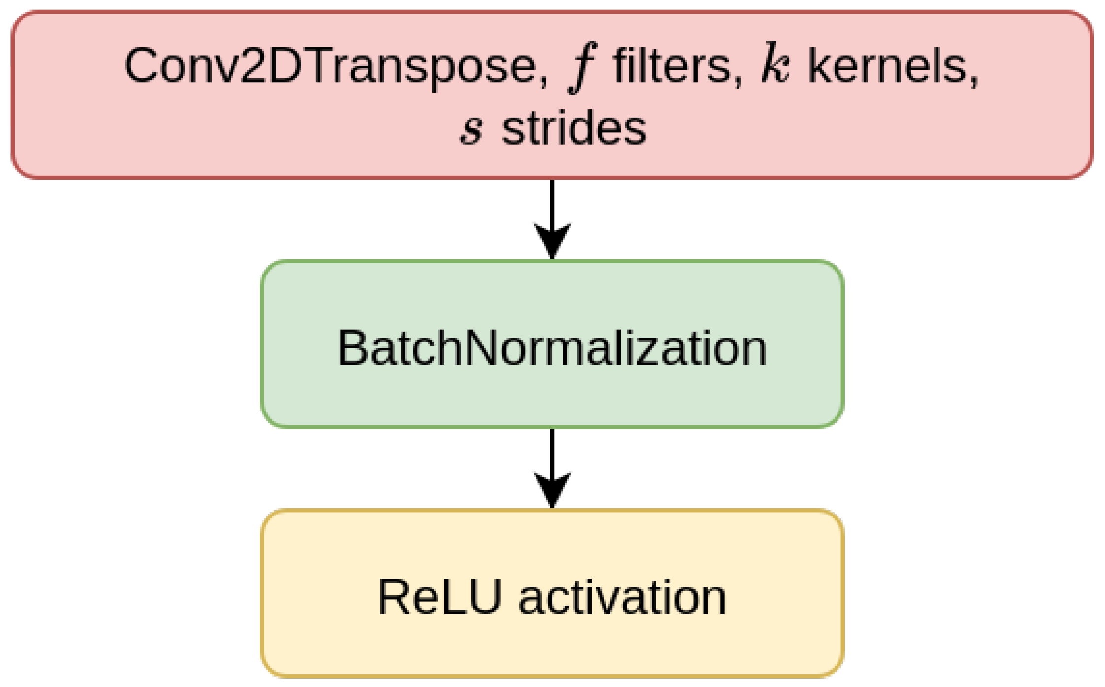
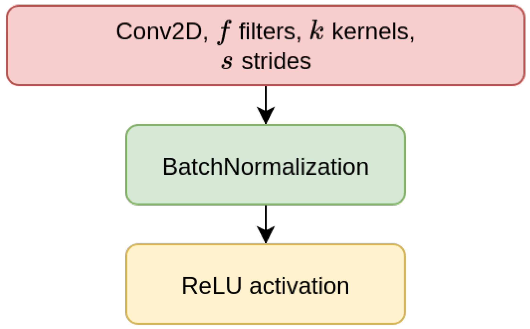
We have considered two types of deep learning models, Contractive Auto-Encoders (CAE) and Convolutional Neural-Networks (CNN), both of which are designed for the task of imputing missing nucleotides in genomic sequences. For each model, we have designed three different architectures which differ for the size of the input sequence they receive as input (either 200, 500, or 1000 nucleotides). This choice is motivated by our will to investigate whether different window sizes bring to different performance. Anyhow, all the models are composed of multiple encoder blocks (EBlock, Figure 1), and each EBlock is composed by one 2D convolutional layer (Conv2D layer) followed by Batch Normalization and ReLU activation [69] (as suggested in [70]). The CAEs also need a decoder sub-module, which is composed of a decoder block (DBlock, Figure 2), where the Conv2D layer is substituted with a transposed (expanding) Conv2D layer [71].
All models use Nadam optimizer [50], with the learning parameters suggested by the authors themselves: learning rate 0.002 , decay 0.004 and the gradient and momentum coefficients are β 1 = 0.9 and β 2 = 0.999 respectively. The CAE models must reconstruct the input sequences of length N, and their output is therefore structured like the input sequence (i.e., N × 4 nodes, four nodes for each one-hot-encoded nucleotide of the sequence, see Section 4.1). The output of the CNN is instead composed of four nodes representing only the one-hot-encoding of the missing nucleotide at the center of the input sequence. For this reason, while the input of both models is the same nucleotide sequences containing gaps, the ground truth labels used during training are different. For the CAE models, we compute the loss by using the input sequence without gaps, while the loss of CNNs only considers the prediction of the central gap.
Both model types use the Softmax activation for the last layer and categorical cross-entropy as the loss function—in the CAE models these functions are applied in their per-axis version (Figure 3a,b). We have used an early-stopping criterion based on the improvement of the validation loss—if no improvement is observed within 10 epochs, the training is interrupted. The maximum possible number of epochs is set to 1000, but we note that using this criterion, no model went over the 100 epochs of training in our experiments. In the following Section 3.1 and Section 3.2 we point out the peculiarities of, respectively, the CAE and the CNN models.

3.1. CAE Model

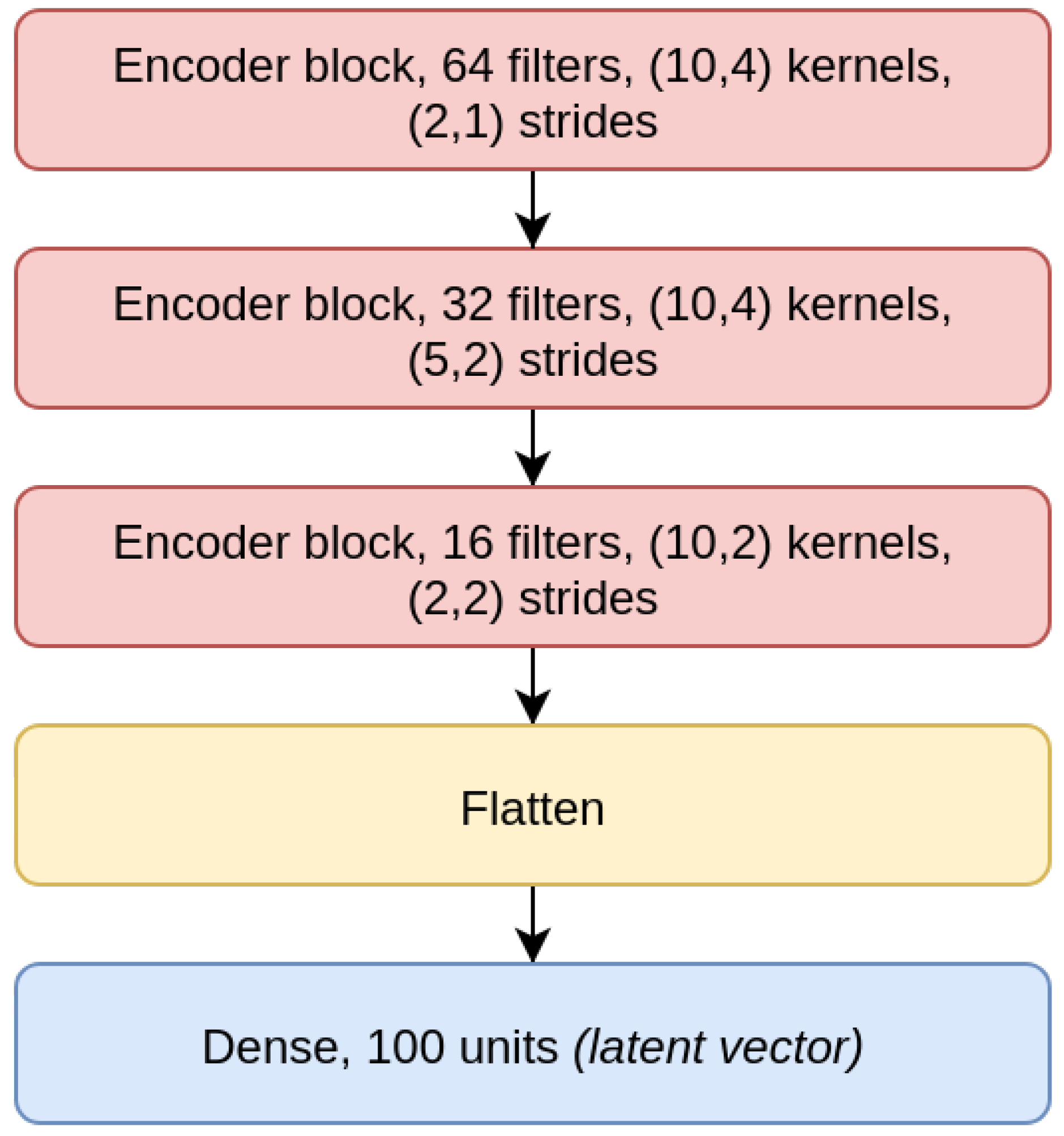
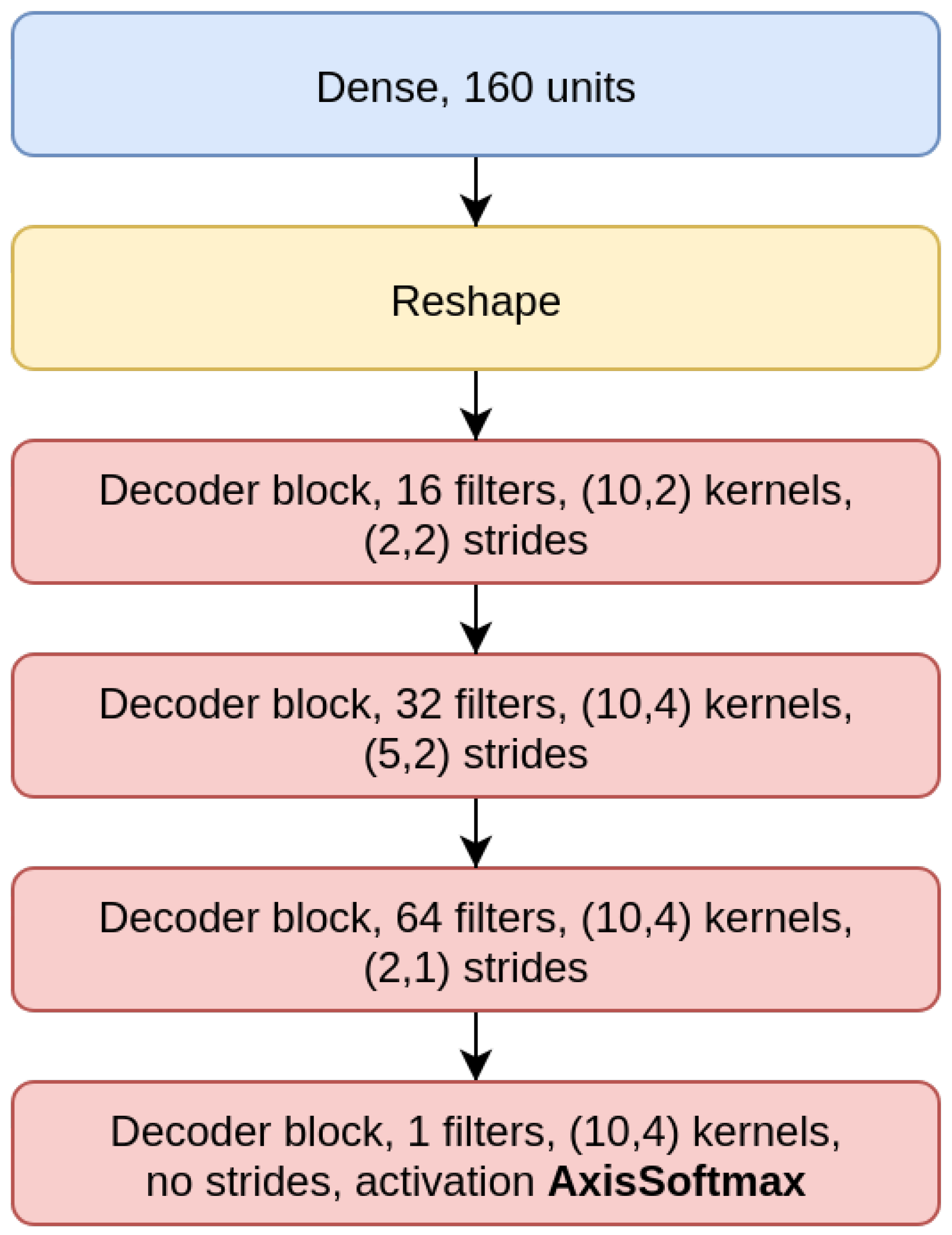
The CAE model is the concatenation of an encoder (Figure 4), composed by three EBlocks (Figure 1), and a decoder (Figure 5), composed of three DBlocks (Figure 2). Between the encoder and the decoder parts, the latent layer is a Dense layer with linear activation, whose goal is to embed the data into a latent lower-dimensional vector space. Depending on the considered window size (200, 500, or 1000), the latent layer has a different number of nodes: 100 nodes for the CAE 200, a latent space of size 150 for CAE 500, and 200 neurons for CAE 1000. All the convolutional layers use the padding “same”, which enforces the same output size padding with zeros. The CAE 200, CAE 500, and CAE 1000 structures are detailed in Table 1.
Note that we use strides instead of max-pooling to reduce the computational load, after considering that the usage of the stride during image recognition tasks on several benchmark datasets [72] introduces no significant loss of accuracy.
Since the CAE model loss has the same impact on all the output nucleotides, the model might learn an identity function and only reconstruct the known input values without actively imputing the gap at the center of the window, which is the one we aim to fill. In order to prevent this, we weigh differently the loss related to the misclassification of nucleotides, based on their position in the window. Precisely, we set a maximum weight at the window center, where we have the missing nucleotide to be imputed, and we linearly decrease it down to 1 as it reaches the borders. The maximal weights considered are w { 1 , 2 , 10 } , where the maximal weight that equals 1 produces an unweighted training.

3.2. CNN Model

To focus entirely on the imputation of the missing value at the center of the input sequence, and to avoid altogether the task of also reconstructing the other nucleotides, we have designed CNN models, which may be considered as truncated CAEs that avoid the data reconstruction after its embedding in a lower-dimensional space and therefore need a significantly lower number of parameters, which allows for faster training and inference. Moreover, when viewed as truncated CAEs, CNNs are characterized by a loss that is weighted with an extremely high value, so that only the misclassification of the central nucleotide is considered.
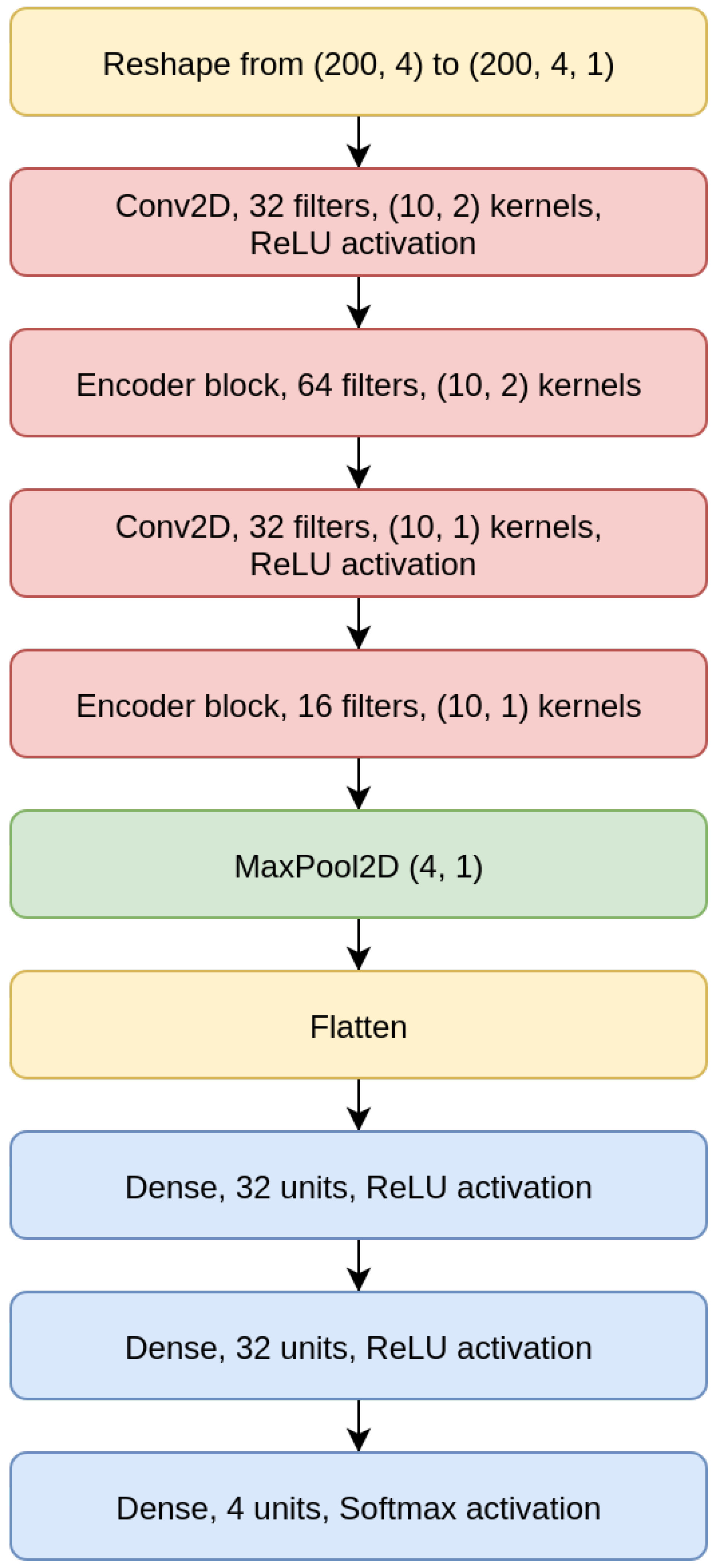
As shown for the CNN 200 model in Figure 6, the CNNs we designed are composed of two convolutional layers intertwined with EBlocks, followed by a MaxPooling and a Flatten layer (a layer that transforms the bi-dimensional output of a convolutional layer into a one-dimensional vector), and then a sequence of Dense layers on top, which terminates with a Dense layer with four output neurons and Softmax activation.
All CNN models use a categorical cross-entropy as loss, and all convolutional layers use padding. The CNN models structures are detailed in Table 2.

4. Experimental Setup

We have applied the proposed deep learners for imputing the missing value at the center of a genome sequence which may contain either no-other gaps (single-gap sequence, see Appendix A.1) or many other gaps (multivariate-gap sequence, see Appendix A.2). We call this task the gap-filling task.
Additionally, we considered the ability of the CAE models to reconstruct the whole sequence when the input sequence is either a single-gap sequence or a multivariate-gap sequence. This task, which we call the reconstruction task, should reconstruct the values already present in the input sequence, that is, the known nucleotides, while simultaneously imputing the missing ones, that is, the nucleotides filling the gaps.
To measure each model performance, we averaged the Categorical Accuracy, the Area Under the Precision Recall Curve (AUPRC) and Area Under the Receiver Operating Characteristic curve (AUROC) scores computed in a one-vs-one fashion (each nucleotide against each other). When evaluating the CAE models on the reconstruction task, all the measures were further averaged over all the nucleotides in the sequence. For each task and each model, we also analyzed the performance on the imputation of each nucleotide, by computing the categorical Accuracy, the AUPRC and AUROC in a one-vs-all fashion, to identify eventual preferential overfitting to one specific nucleotide class. The statistical significance of all the comparisons has been validated by a Wilcoxon signed-rank test [73] (at the 95% confidence level, that is, p-value less than 0.05 ); the Wilcoxon validation has allowed to compare and summarize all the computed performance through Win-Tie-Loss tables (a tie is detected when the Wilcoxon does not detect a significant difference in the compared performance). The same 95% confidence level has also been used for the Pearson correlation tests [74], and the Spearman correlation tests [75], which have been used to correlate the achieved performance to the size of the input sequence.
The single-gap, multivariate gap, and biological datasets, which have been used to train, test, and validate our models for both the gap-filling and the reconstruction task, are composed of genome sequences from the reference assembly hg19, the penultimate reference human genome, where we artificially inserted gaps.
As explained in detail in Appendix A.1 and Appendix A.2, starting from sequences with no gaps in hg19, we have generated a single-gap dataset (see Appendix A.1), which contains sequences where only the central nucleotide has been removed, and a multivariate-gap dataset (see Appendix A.2), which contains the single-gap sequences where many other gaps have been artificially inserted in a way that resembles the biological gaps found in the human genome. To visually assess such similarity, Figure 7-center and Figure 7-right show, respectively, the frequencies of the gaps in the multivariate-gap dataset we generated, and the frequency of the gaps in the hg19 sequences we considered for generating the statistical gap model. Moreover, we computed both the Pearson correlation coefficient (0.974, p-value ≈ 0), as well as the Spearman correlation coefficient (0.998, p-value ≈ 0) between such frequencies; both coefficients highlight the high correlation between the two signals.
To validate our results, we further composed a biological dataset (Appendix A.3) which contains the few sequences with single nucleotide gaps in hg19 that were filled in the most recent reference assembly, hg38. The generated single-gap and multivariate-gap datasets have extremely high cardinality, while the biological dataset is considerably smaller (see Table 3).

4.1. Sequence Data Coding

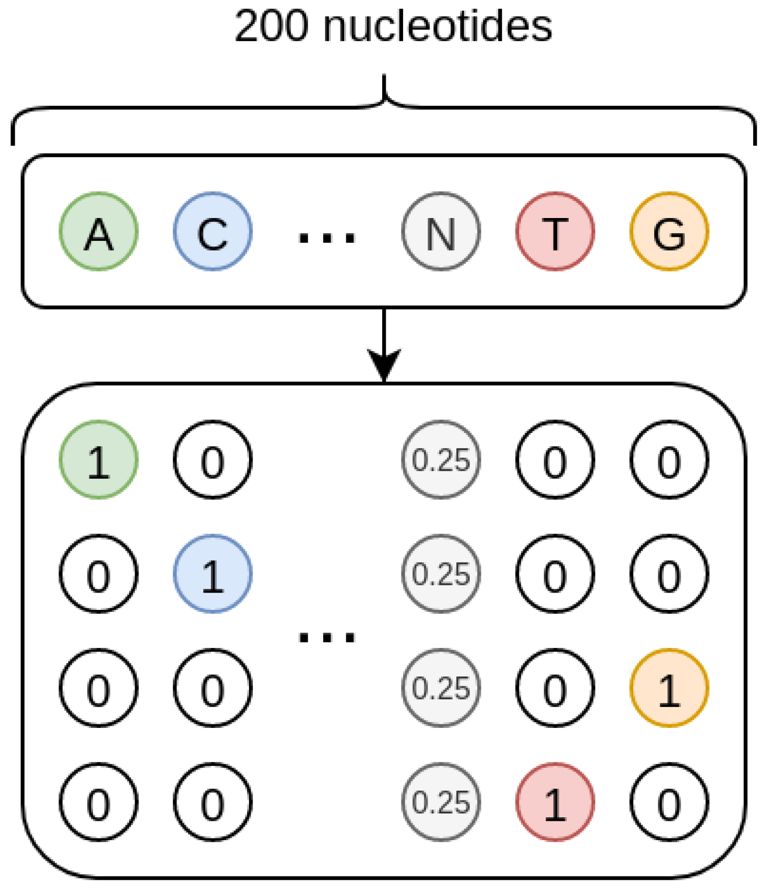
As shown in Figure 8, the sequences we treat are one-hot encoded, and each missing nucleotide is represented by a 4D vector where all the elements have value 0.25. In such a way, the one-hot encoding procedure inherently encodes a probability. Indeed, when the nucleotide is present, its probability is 1 while that of the other nucleotides is 0; when the nucleotide is missing, the uniform probability distribution is used, so that all the four nucleotides have the same probability.
For the CAE models, this probability setting could be interpreted as a Bayesian framework where the input one-hot encoded sequences would be viewed as the priors, and the model would learn to compute the posteriors by internally modelling the conditional probability that a nucleotide is in a specific position in the sequence given the neighbouring nucleotides.

4.2. Training, Test, and Validation Partitions

While the sequences in the biological dataset are only used for validating the models, the single-gap and multivariate-gap sequences are used for training and testing. For this reason, we have split the available sequences into train and test set by using a randomly generated chromosomal holdout to avoid positional bias caused by samples from the same chromosome.
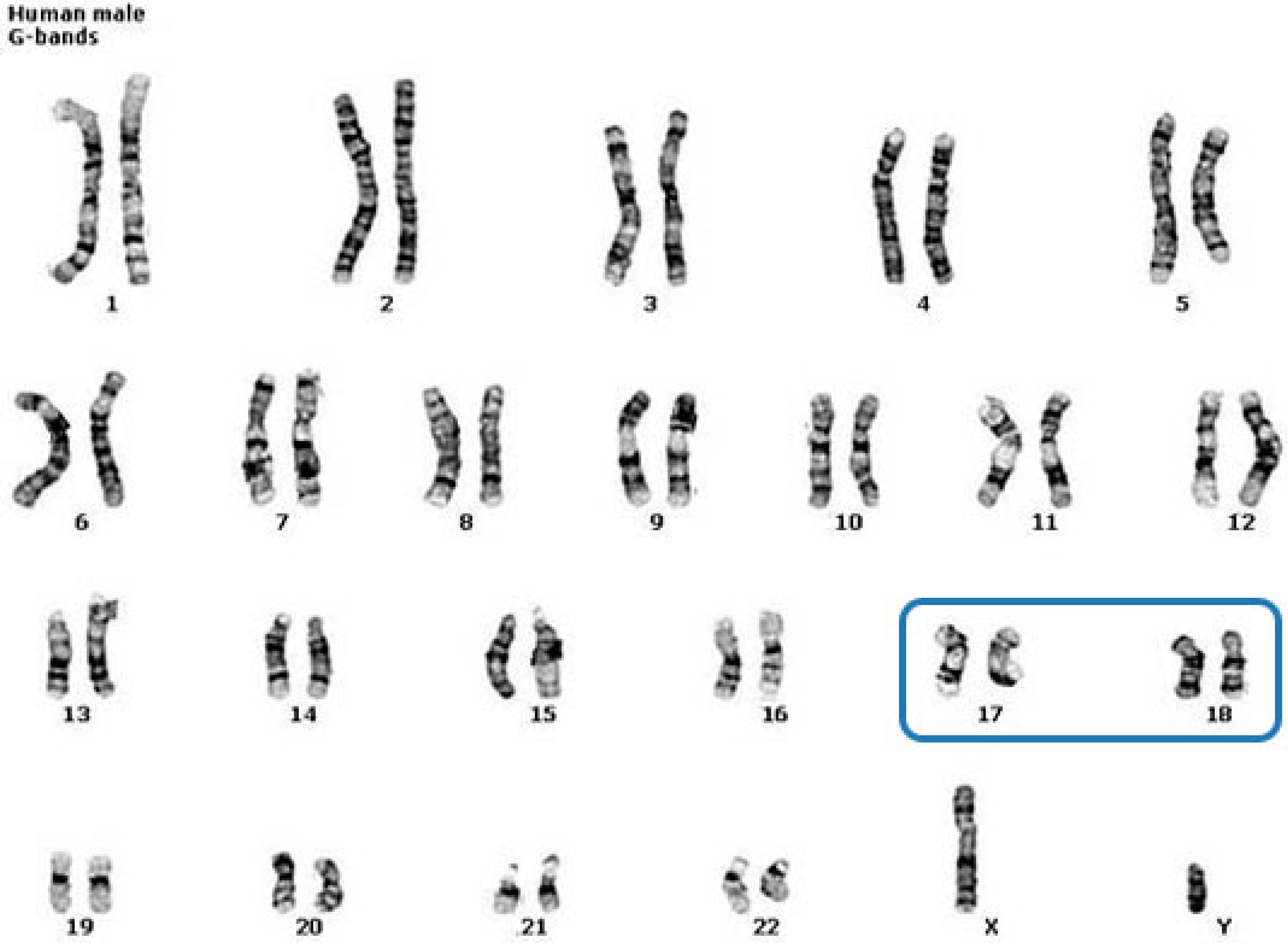
Precisely, we have randomly selected 17 and 18 chromosomes for testing, and we have used the other chromosomes for training (Figure 9). Both train and test partitions contain a considerable amount of sequences (Table 3). The test-train cardinality proportion is ≈17.97%. As detailed in Table 3, when comparing the number of gaps corresponding to each of the four nucleotides, the train and test sets from the single-gap and multivariate-gap datasets are only slightly unbalanced, while the biological dataset contains highly unbalanced proportions of missing nucleotides.
Since, for each model, we also wanted to assess the model robustness with respect to the number of gaps viewed during training, we evaluated two instances for each model. The first instance is obtained by training the model on the training sequences with only one gap at the center (single-gap training set); this instance is evaluated on a validation set composed by all the other unseen (single-gap and multivariate-gap) sequences, independently on the number of gaps (that is, this instance is tested both on sequences in the single-gap test set, and on all the sequences with more than one gap, and belonging to the multivariate train and test sets). Similarly, the second instance of the model is trained by using the sequences with many gaps in the multivariate-gap training dataset, and is tested on the validation set composed by all the other not-seen sequences (single-gap train and test sequences plus multivariate-gap test sequences). Of course, the two instances are also tested on all the sequences in the biological dataset.
In this way, for each instance of the model, we obtain five evaluations (shown separately in the next Section 5): the evaluation on the set used for training, which provides a first evaluation of the model generalization or overfitting, the evaluation of the results obtained on all the three sets in the validation set, and the assessment on the biological dataset.
All the data generation code and the deep models are available for research purposes at the public repository on GitHub (https://github.com/LucaCappelletti94/repairing_genomic_gaps). All the deep models have been implemented using Keras/TensorFlow [76,77] and the trained models are available in the GitHub repository. Note that all the code has been optimized in order to reduce both the memory requirements as well as the computational time so that the experiments may run on consumer-grade computers equipped with a GPU.

5. Results

We present our results starting with the performance of the CAE models when applied to the gap-filling task, which aims at imputing the central nucleotide (Section 5.1); then, we present the models’ performance on the reconstruction task, where the entire input sequence is reconstructed and filled (Section 5.2). Subsequently, we report the results obtained by the CNN models in the gap-filling task (Section 5.3), and we conclude by reporting the comparative evaluation between the best CAE and CNN models in the gap-filling task, where we use as a benchmark the gap-filling results achieved by the KNN-imputation method proposed in Troyanskaya et al. [8].
KNN-imputation has been chosen due to its wide application in several fields [29,78,79,80,81] and to its successful results when imputing epigenomic data generated from DNA micro-arrays. The setting of the KNN-imputation parameters that is the employed distance function and the number of neighbours, are described in detail in Section 5.4.
Note that we also tried to run the ML imputation approach, based on Random Forests and presented in Stekhoven et al. [14]. However, the computational load required by the python implementation we used made it impracticable (In our experiments, we used the implementation of KNN-imputation from scikit-learn [82], while the MissForest implementation is available at Missingpy).

5.1. CAE—Gap-Filling

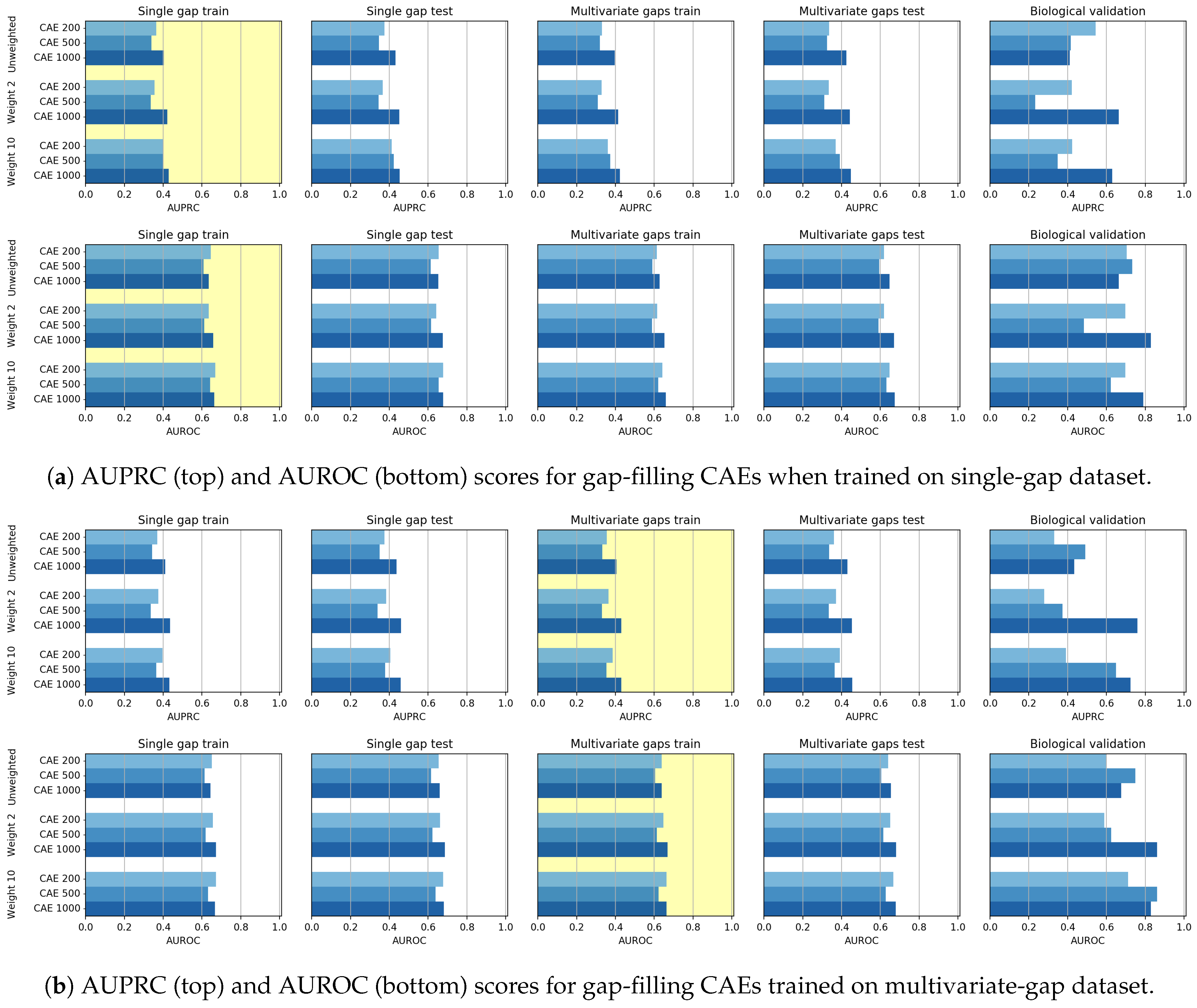
In Figure 10 we visually compare the results achieved by all the CAE models, which differ for both the size of the input sequence ( { 200 , 500 , 1000 } ) and the linear weight ( w = { 1 , 2 , 10 } ) applied during training (as detailed in Section 3.1). In Figure 10a,b the yellow backgrounds highlight the results on the datasets used for training, which are, respectively, the single-gap dataset and the multivariate-gap dataset.
To assess the statistical significance of the achieved performance, in this Section and in the following ones, we apply the Wilcoxon rank-signed test at the 95% confidence level, by considering only the results achieved on the validation set, composed by all the unseen sequences, but excluding the results on the biological set for it has an insignificant number of sequences when compared to the other sets. Precisely, the Win-Tie-Loss Table 4 shows the comparison between the results achieved on the validation sets by all the CAE models grouped according to their weights, while the Win-Tie-Loss Table 5, shows the comparison between the results of the CAE models with differing input sizes.
Comparing the CAEs being differently weighted, we see from Figure 10 and from Table 4 that the CAE with weight 10 outperforms the other models in the validation set. However, in the biological set the CAE 1000 with weight 2 is always the best performing model (rightmost sub-figures in Figure 10), both when considering the instance trained on the single-gap sequences (Figure 10a) and when considering the one trained on the multivariate ones (Figure 10b).
This suggests that the input size has a great impact on the achieved performance. Indeed, both Figure 10 and Table 5 highlight that the CAE 1000 is the best performing model. To further support the better performance of the CAEs having a larger input sequence, we have verified the high correlation between the achieved evaluation and the input size through the Pearson and Spearman correlation coefficients (see Table 6, where we show also the p-values witnessing the statistical significance of the computed Pearson and Spearman correlation coefficients).
The higher performance of CAEs with larger input size may be due to the fact that the input sequence carries more information than that carried by shorter sequences, and therefore better describes the relationships between neighboring nucleotides.
We further investigated the gap-filling performance on each nucleotide (see Table 7) through the Wilcoxon rank-signed test applied on the results achieved over the validation set (see the Win-Tie-loss Table 8). Though Adenine and Thymine seem having a much lower accuracy, and consequently a lower AUROC, their AUPRC is higher, as also shown by the Wilcoxon rank-signed test (see Table 8). We, therefore, conclude that the models achieve comparable results on each nucleotide.

5.2. CAE—Reconstruction

When the CAE models are applied for sequence reconstruction, we note a different behaviour. At first, the observation of both Figure 11 and of the Win-Tie-Loss Table 9 show that, as expected, the weighting applied during training does not influence the achieved performance. Secondly, we note an inverse correlation between the length of the input sequence and the reconstruction results. Indeed the Win-Tie-Loss Table 10 and the Pearson and Spearman correlation coefficients (Table 11 and Table 12) highlight that the CAE 200 is the best performing model on the validation set, followed by the CAE 500 and CAE 1000. This behaviour may be because the reconstruction power is dispersed on the whole sequence; the longer the sequence, the more dispersed is the CAE generalization capability.
Analyzing the reconstruction performance of each nucleotide separately (Table 13) we note that Adenine seems to be the nucleotide achieving the worst reconstruction result, as also confirmed by the Wilcoxon Win-Tie-Loss Table 14, where Adenine is the unique nucleotide having the highest number of losses over the three evaluation measures. Finally, we report the Win-Tie-Loss Table 15, which compares the performance of all the CAEs (in both the gap-filling and reconstruction task) when they are trained on the single-gap or the multivariate-gap dataset. The table highlights that there is no statistically significant difference between the achieved results. CAE models are, therefore, robust concerning the number of gaps in the input sequence.

5.3. CNN—Gap-Filling

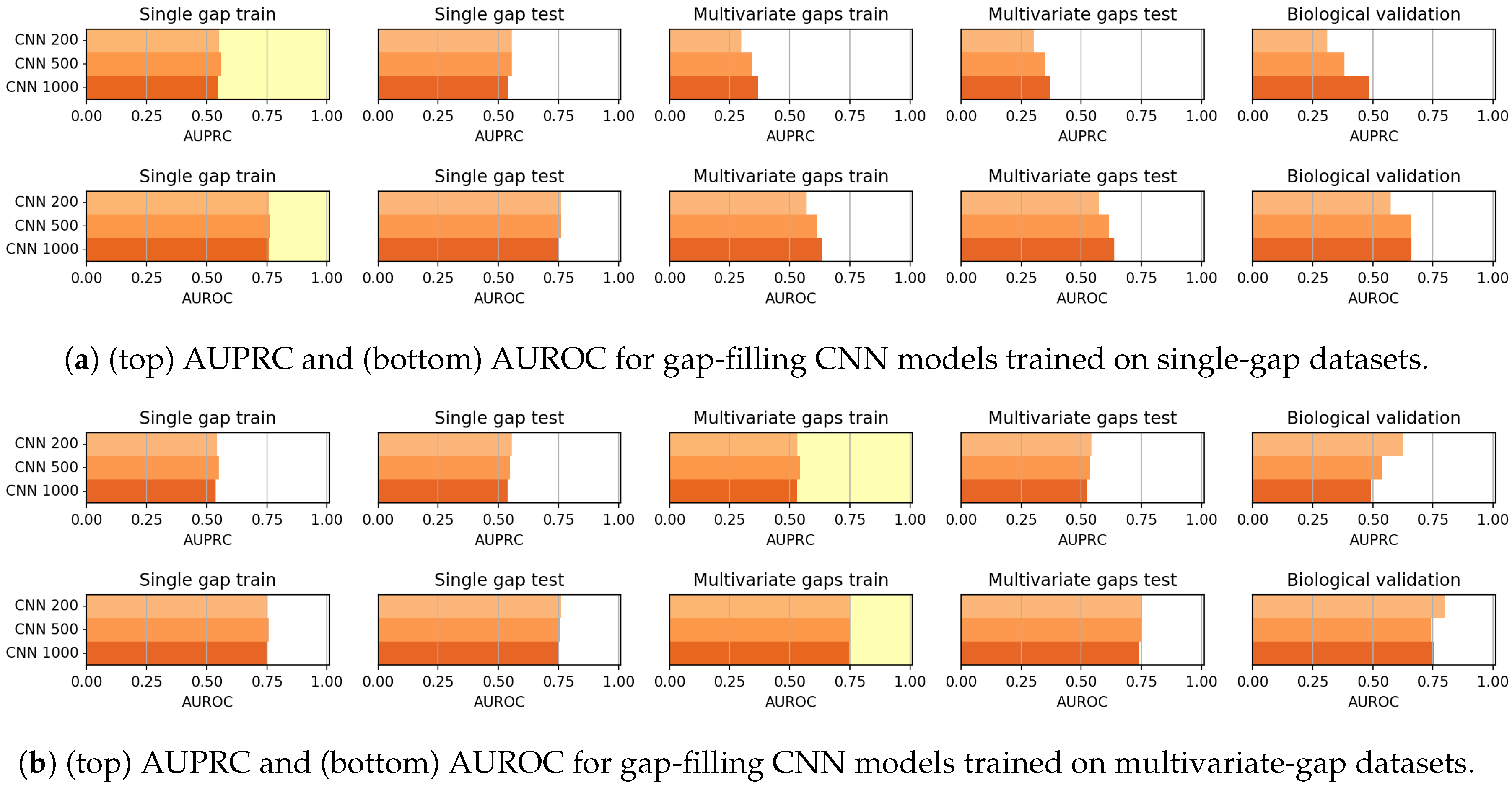
In Figure 12 the results achieved by CNN models when trained on the single-gap sequences (Figure 12a) and on the multivariate-gap sequences (Figure 12b) are shown. Firstly the CNN models, differently from the CAE models, do not show any correlation between the window size and the gap-filling performance (see Table 16 and Table 17). Moreover, the behaviour of CNNs varies when either the single-gap or the multivariate-gap dataset are used for training. Indeed, as also confirmed by the Wilcoxon rank-signed test at 95% confidence level (summarized by the Win-Tie-Loss Table 18), the use of the multivariate-gap dataset for training improves the metrics on the validation set composed by the unseen sequences (excluding the biological set). For what regards the comparison on each nucleotide, as it happens for the CAE models, the performance of the gap-filling CNNs are comparable (see Table 19 and Table 20).

5.4. Models Comparison

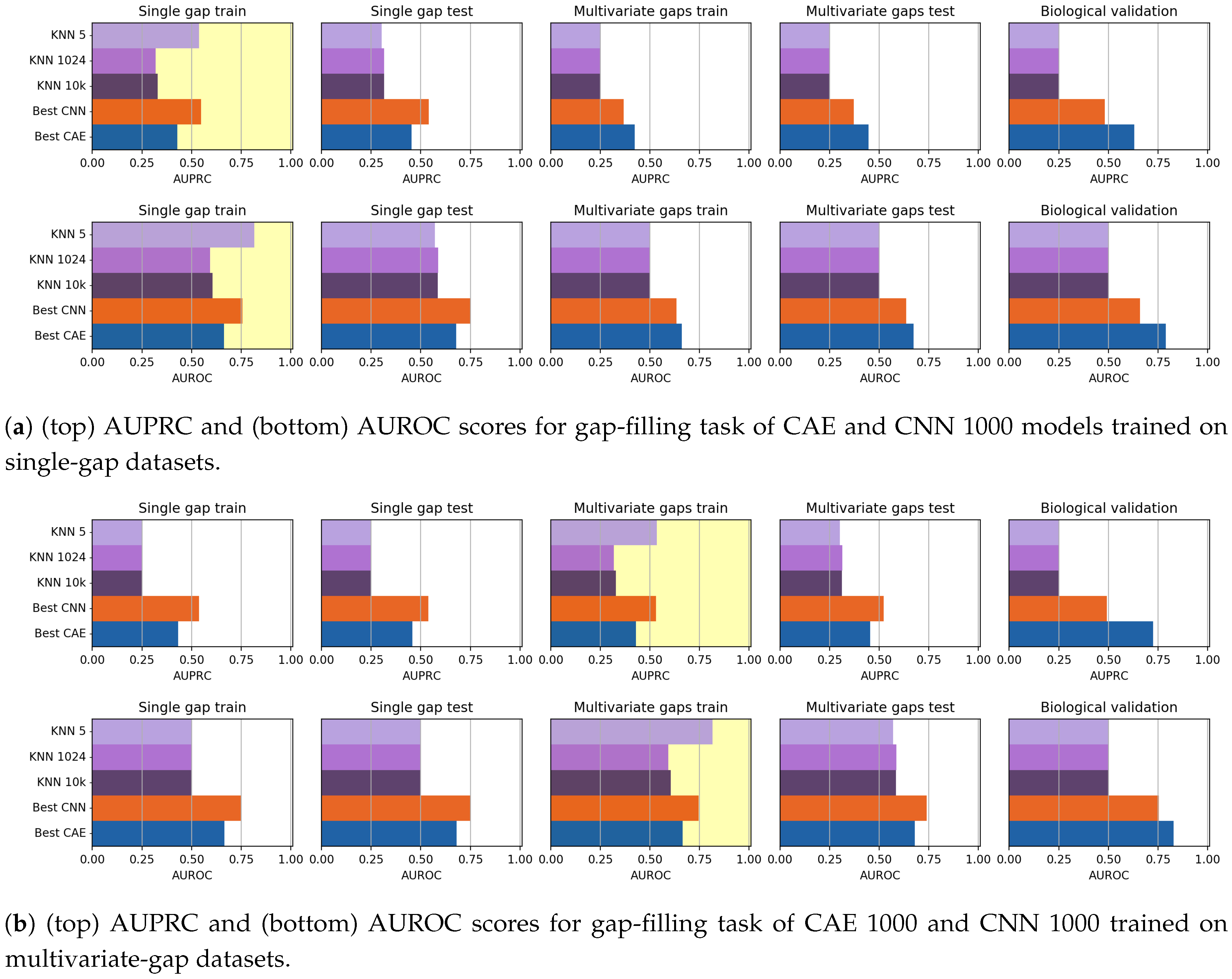
We ran our comparative evaluations by using all the considered data (including the biological dataset). To compare the gap-filling performance of CAEs and CNNs, we considered the CAE 1000 model, for it is the best-performing among the CAE models we tested, and we chose the CNN 1000 model, to provide a fair comparison by using sequences with the same input size and after considering that the performance of the CNN models is independent on the length of the input sequence. To compare the results achieved by our models to a benchmark state-of-the-art method, in this section, we also show the results achieved by the KNN-imputation method [8] described in Section 2. When using the KNN-imputation, the distance between sequences (used to search for the k neighbours) is the euclidean distance, as proposed by the authors. When computing the pairwise distances, if the i t h value is missing for one of the two sequences, such term is not considered in the distance computation. Due to the impracticable computational load required by the KNN-search, both the training and the test sets have been reduced to 40,000 randomly selected sequences. To choose the number of nearest-neighbours that maximizes the gap-filling AUPRC value, we run several tests by varying the value of k. Anyhow, when running our test we noted that, though lower values of k seem to produce a higher gap-filling performance on the training set, both small and huge k values produce the same results on the validation set. For this reason, we show results achieved by using both k = 5 , and k = 1024 , and k = 10,000 neighbors. In Figure 13, the gap-filling performance achieved by all the models are visually compared. Regarding the models trained on the single-gap dataset (Figure 13a), we note that, while the 5-nn imputation model achieves the best results on the training set when it is validated on the unseen datasets, its performance is as low as those of the other KNNs. Surprisingly, the CAE 1000 seems to perform slightly better than the CNN 1000, even on the biological dataset. On the multivariate dataset (Figure 13b), 5-nn imputation again has a dramatic drop of performance when going from the training to the validation sets. Here the CNN 1000 seem to perform slightly better than CAE 1000 on all the datasets, except for the biological validation set. Indeed, on the biological dataset, the CAE 1000 is the best performing classifier. To understand if there is a significant difference between the CAE 1000 and the CNN 1000 performance, we, therefore, applied a Wilcoxon rank-sign test at the 95% confidence level by considering the results on the validation set (biological set excluded), and we obtained the Win-Tie-Loss Table 21. In the table, the two losses of all the KNN-imputers are obtained in comparisons with the CAE 1000 and CNN 1000, while the ties are in comparisons with the other KNN imputers. The tie obtained by the CAE 1000 is in comparisons with the CNN 1000, and vice-versa. The Wilcoxon tests, therefore, confirm that CAE 1000 and CNN 1000 outperform all the KNN instances.

6. Discussions, Conclusions and Future Works

In this paper, we have investigated the usage of CAEs and CNN for the task of missing data imputation in complex datasets. The proposed deep-learning imputation methods have been successfully applied on genome datasets for filling the missing nucleotides (gap-filling task) or for reconstructing entire genome sequences while simultaneously filling their gaps (reconstruction task). Our experiments have shown that both CAEs and CNNs outperform KNN-imputation, a widely used state-of-the-art technique.
Precisely, the promising results achieved by the CAEs suggest that the lower-dimensional representation expressed in the latent space retains all the salient information required for describing the structure of the input sequence, as it is needed in this case study. For this reason, our future works will be aimed at applying the CAES for supporting classification tasks. Precisely, by training the CAEs for a specific classification task, we could obtain more discriminative representations in the latent space, which could be used as input to other discriminating algorithms [85,86].
Though the CAE models obtained promising reconstruction results, after experimenting their gap-filling capability we experienced poorer results when compared to CNNs, probably meaning that the network learning ability is dispersed with the aim of producing a good reconstruction of the whole sequence. We, however, noted that when the size of the input sequence increases, the CAE performance increases. Moreover, for what regards the gap-filling task, our proposal of weighing the central nucleotide differently is promising since it allows increasing the gap-filling performance.
As mentioned before, the CNN models generally outperformed the CAE models in the gap-filling task. On the other hand, the validation of the Biological dataset shows that CAE is competitive with CNN, but the reduced cardinality of the dataset suggests particular caution in drawing conclusions.
Anyhow, both models achieved promising results which we believe are robust with respect to the parameters settings.
Indeed, the only evident critical parameter we introduced in this work, is the weight of the AE, which allows weighing more the imputation performance of the missing element. To test the criticality of the weight setting, we have shown experiments where completely different weight values are used. The reported results show that, indeed, the AE should give more importance to the reconstruction of the element that must be imputed. Therefore, by observing the achieved results it is easy to set the best weight value.
The other parameters that may influence the achieved performance, are those related to the training algorithm (Nadam optimizer [50]). Regarding their choice, we used the settings proposed by the Nadam author themselves. The author’s parameter setting was a two-fold decision—he chose the parameter setting allowing to achieve a good stable performance (negligible performance variations are visible when the parameter values are varied in the neighborhood of the chosen values).
Anyhow, the promising results obtained by both the models, and our awareness that the stability of our performance with respect to the parameter setting could not be valid for the specific problem being tackled, motivate our future works aimed at further improving performance by searching for the best hyperparameter settings in a wider hyper-parameter space. Parameter search may be performed by random search [51], or Bayesian optimization [52], which have proven to effectively find an optimal setting [48].
Anyhow, considering both the CAEs and CNN results, auto-encoder models seem to provide useful and informative data embedding, while the CNN models could seem promising gap-filler. Natural future work could, therefore, be aimed at integrating U-Nets auto-encoders and CNNs, optimized through bayesian search, to obtain a novel structure exploiting the strengths of both the architectures.
Eventually, we could even modify the deep convolutional architecture, by substituting it with a Recurrent Neural Network [87].
Finally, we note that the gap filling application presented in this paper is a Proof of Concept, to show how deep imputers may be successfully applied to solve the problem of the complex-data imputation. In this case, the architecture of the proposed techniques has been designed to adhere to the chosen complex categorical data. For this reason, the presented deep learner process a 2D binary (one-hot-encoded) input and are constituted of internal layers using 2D convolutional filters, which are the most appropriate for this problem, and an output layer with one node for each category. After opportunely diminishing/augmenting the number columns in the input layer and the number of nodes in the output one, the presented techniques could be retrained to fill the gap of any other type of complex categorical dataset, where convolutional filtering is appropriate. Note that when convolutional filters are not appropriate, dense layers could be used.
On the other hand, if (2D or 1D) continuous complex data should be imputed, both the input layers, and the internal filters should be adapted to the input dimension (1D convolutional filters or 1D dense layers for 1D input, and 2D filters or 2D dense layers for 2D input), while the multi-node output should be substituted by a unique node containing the value of the missing element. Of course, in this case, the same training procedure would result in a regressor rather than in a classifying machine (since the predicted categorical data would be substituted by a continuous value). Our future works will be aimed at testing the deep imputers for application where continuous complex data (e.g., epigenomic data) must be imputed.

Author Contributions

L.C., T.F.: software implementation; L.C., T.F., G.W.D.D., L.D.T.: dataset creation; L.C., T.F., E.C., G.V.: research design, experimental evaluation design, algorithm evaluation, article writing, article revision. All authors have read and agreed to the published version of the manuscript.

Funding

This research was funded by Università degli Studi di Milano, PSR2019_DIP_010_GVALE: Machine Learning and Big Data Analysis for Bioinformatics.

Conflicts of Interest

The authors declare no conflict of interest.

Abbreviations

The following abbreviations are used in this manuscript:
AEAutoencoder
CAEContractive Autoencoder
CNNConvolutional Neural Network
AUROCArea Under the Receiver Operating Characteristic curve
AUPRCArea Under the Precision Recall Curve
Conv2D2D Convolutional Layer
Conv2DT2D Transposed Convolutional Layer
ReLURectified Linear Unit
NADAMNesterov ADAptive Momentum estimator
UCSCUniversity of California Santa Cruz
EBlockEncoder Block
DBlockDecoder Block

Appendix A. Genome Sequence Datasets

In this appendix, we firstly explain how we artificially generated the (single-gap) sequences, which contain only one gap at the center of the sequence (see Appendix A.1), and the multivariate-gap sequences, which contain many gaps other than the gap at the center of the window (see Appendix A.2).
Further, we detail how we extracted the biological dataset (see Appendix A.3), which contains the few sequences with only one gap in hg19, that were filled in the most recent reference assembly, hg38.

Appendix A.1. Single-Gaps Sequences

To generate the dataset with single-nucleotide gaps, we downloaded hg19 and extracted the regions without gaps (using UCSC genomes downloader). For each considered sequence length ( = { 200 , 500 , 1000 } ) , we tessellated these regions into smaller sequences of length (window size), and we replaced the central nucleotide of each extracted sequence (nucleotide-window) with a gap.

Appendix A.2. Synthetic Multivariate Nucleotides Gaps

To create a dataset containing sequences with many gaps, we have tried to approximate the frequency of the biological gaps in the genome sequences in hg19, by estimating a model of the gap positions found in hg19 through a multivariate Gaussian distribution. To estimate the parameters of such Gaussian distribution (mean and covariance) from the biological gaps present in hg19, we have used the following procedure.
We firstly identified all the single nucleotide gaps available in hg19 (which are 51), and we expanded their genome region up to the length ( = { 200 , 500 , 1000 } ) of the considered window size. We then stacked the 51 sequences (one on top of the other) to compose a Boolean matrix, with size 51 × , where the true values are in the position of missing nucleotides. We finally computed the mean and covariance and used it to generate a multivariate Gaussian. For each sequence, we then sampled values from the estimated multivariate Gaussian and we thresholded such (continuous) values using a cutoff at t = 0.4 , so that values greater than t become gaps. Note that the threshold value t = 0.4 has been experimentally set to maximize the correlation between the frequency of the artificially inserted gaps (see Figure 7-center) and the frequency of the gaps in the human hg19 genome (see Figure 7-right). Indeed, both the Pearson correlation value (0.974, p-value 0 ) and the Spearman correlation value (0.998, p-value 0 ) confirmed that the artificially inserted gaps have a frequency resembling that of human genome.

Appendix A.3. Biological Validation Dataset

The biological dataset is composed of 19 sequences generated by filling the single-nucleotide gaps found in the assembly hg19 with the corresponding nucleotides found in the assembly hg38, as can be retrieved from the UCSC genome browser. The low cardinality of this dataset is due to the fact that we could only select a small number of single-nucleotide gaps of hg19 that were actually filled in hg38, while the majority of such gaps found on hg19 still remain unresolved in hg38. To generate the biological validation dataset, we have employed the procedure illustrated in Figure A1. First, we have identified all single-nucleotide gaps in the genomic assembly hg19 and we have selected their 800 bp neighborhoods (Figure A1a). Then, for each gap, we have computed the best local alignment of its neighborhood on hg19 to the whole corresponding chromosome of hg38 (Figure A1b), in order to be sure to actually retrieve the best local alignment within the chromosome. To this aim, we employed Huxelerate technology (available through an API called Hugenomic [88]), which speeds up the task of aligning genomic sequences exploiting FPGA architectures.
After finding the regions of hg38 matching the 800 bp neighborhoods of hg19 gaps, our procedure retrieves the nucleotides of hg38 in the positions occupied by the “N” characters (i.e., gaps) in hg19. To do this, for each hg19 gap, we select the 200 bp right neighborhood (RN) and the 200 bp left neighborhood (LN), as shown in Figure A1c. Then we perform 2 semi-global alignments, which will be referred as RN-alignment and LN-alignment, to align, respectively, the RN and LN regions of the hg19 assembly to the (previously identified) region of hg38 (Figure A1d). If the distance between the last position of hg38 covered by the LN-alignment (namely LL) and the first position of hg38 covered by the RN-alignment (namely FR) is equal to the length of the gap in hg19 (1bp in our case), then we are sure that the nucleotide between LL and FR correspond to the “N” in hg19 (Figure A1e).
For gaps where the distance between LL and FR in hg38 is not equal to the length of the gap in hg19, we output the LL and FR positions and proceed to a manual evaluation (Figure A1f). When we were able to manually retrieve the filler sequences, we added a new “observation” to the already generated dataset.
Figure A1. Procedure for generating the biological validation dataset. (a) Gap identification and neighborhood selection. (b) Identification of the corresponding region on hg38 (local alignment).(c) Selection of right (RN) and left neighborhood (LN) on hg19 fragment. (d) Semi-global alignment of RN and LN on hg38 fragment. (e) Distance between aligned regions is equal to gap length: filler sequence is automatically retrieved. (f) Distance between aligned regions not equal to gap length: filler sequence is not automatically retrieved.
Computers 09 00037 g0a1

References

  1. Osman, M.S.; Abu-Mahfouz, A.M.; Page, P.R. A Survey on Data Imputation Techniques: Water Distribution System as a Use Case. IEEE Access 2018, 6, 63279–63291. [Google Scholar] [CrossRef]
  2. García-Laencina, P.J.; Sancho-Gómez, J.L.; Figueiras-Vidal, A.R. Pattern classification with missing data: A review. Neural Comput. Appl. 2010, 19, 263–282. [Google Scholar] [CrossRef]
  3. Silva-Ramírez, E.L.; Pino-Mejías, R.; López-Coello, M.; de-la Vega, M.D.C. Missing value imputation on missing completely at random data using multilayer perceptrons. Neural Netw. 2011, 24, 121–129. [Google Scholar] [CrossRef] [PubMed]
  4. Jansen, I.; Hens, N.; Molenberghs, G.; Aerts, M.; Verbeke, G.; Kenward, M.G. The nature of sensitivity in monotone missing not at random models. Comput. Stat. Data Anal. 2006, 50, 830–858. [Google Scholar] [CrossRef]
  5. Scheet, P.; Stephens, M. A fast and flexible statistical model for large-scale population genotype data: Applications to inferring missing genotypes and haplotypic phase. Am. J. Hum. Genet. 2006, 78. [Google Scholar] [CrossRef] [PubMed] [Green Version]
  6. Di Mauro, C.; Steri, R.; Pintus, M.A.; Gaspa, G.; Macciotta, N.P.P. Use of partial least squares regression to predict single nucleotide polymorphism marker genotypes when some animals are genotyped with a low-density panel. Animal 2011, 5, 833–837. [Google Scholar] [CrossRef]
  7. Di Mauro, C.; Cellesi, M.; Gaspa, G.; Ajmone-Marsan, P.; Steri, R.; Marras, G.; Macciotta, N. Use of partial least squares regression to impute SNP genotypes in Italian cattle breeds. Genet. Sel. Evol. 2013, 45, 15. [Google Scholar] [CrossRef] [Green Version]
  8. Troyanskaya, O.; Cantor, M.; Sherlock, G.; Brown, P.; Hastie, T.; Tibshirani, R.; Botstein, D.; Altman, R.B. Missing value estimation methods for DNA microarrays. Bioinformatics 2001, 17, 520–525. [Google Scholar] [CrossRef] [Green Version]
  9. Kalton, G. Compensating for Missing Survey Data; Survey Research Center, Institute for Social Research, The University of Michigan: Ann Arbor, MI, USA, 1983. [Google Scholar]
  10. Owen, A.B.; Perry, P.O. Bi-cross-validation of the SVD and the nonnegative matrix factorization. Ann. Appl. Stat. 2009, 3, 564–594. [Google Scholar] [CrossRef] [Green Version]
  11. Hunt, L.; Jorgensen, M. Mixture model clustering for mixed data with missing information. Recent Developments in Mixture Model. Comput. Stat. Data Anal. 2003, 41, 429–440. [Google Scholar] [CrossRef]
  12. Lin, T.I.; Lee, J.C.; Ho, H.J. On fast supervised learning for normal mixture models with missing information. Pattern Recognit. 2006, 39, 1177–1187. [Google Scholar] [CrossRef]
  13. Steele, R.J.; Wang, N.; Raftery, A.E. Inference from multiple imputation for missing data using mixtures of normals. Stat. Methodol. 2010, 7, 351–365. [Google Scholar] [CrossRef] [PubMed] [Green Version]
  14. Stekhoven, D.J.; Bühlmann, P. MissForest—non-parametric missing value imputation for mixed-type data. Bioinformatics 2012, 28, 112–118. [Google Scholar] [CrossRef] [PubMed] [Green Version]
  15. Marseguerra, M.; Zoia, A. The AutoAssociative Neural Network in signal analysis: II. Application to on-line monitoring of a simulated BWR component. Ann. Nucl. Energy 2005, 32, 1207–1223. [Google Scholar] [CrossRef]
  16. Marwala, T.; Chakraverty, S. Fault classification in structures with incomplete measured data using autoassociative neural networks and genetic algorithm. Curr. Sci. 2006, 90, 542–548. [Google Scholar]
  17. Qiao, W.; Gao, Z.; Harley, R.G.; Venayagamoorthy, G.K. Robust neuro-identification of nonlinear plants in electric power systems with missing sensor measurements. Eng. Appl. Artif. Intell. 2008, 21, 604–618. [Google Scholar] [CrossRef]
  18. Miranda, V.; Krstulovic, J.; Keko, H.; Moreira, C.; Pereira, J. Reconstructing missing data in state estimation with autoencoders. IEEE Trans. Power Syst. 2011, 27, 604–611. [Google Scholar] [CrossRef] [Green Version]
  19. Krstulovic, J.; Miranda, V.; Costa, A.J.S.; Pereira, J. Towards an auto-associative topology state estimator. IEEE Trans. Power Syst. 2013, 28, 3311–3318. [Google Scholar] [CrossRef]
  20. Choudhury, S.J.; Pal, N.R. Imputation of missing data with neural networks for classification. Knowl. Based Syst. 2019, 182, 104838. [Google Scholar] [CrossRef]
  21. Pathak, D.; Krahenbuhl, P.; Donahue, J.; Darrell, T.; Efros, A.A. Context encoders: Feature learning by inpainting. In Proceedings of the IEEE Conference on Computer Vision and Pattern Recognition, Las Vegas, NV, USA, 27–30 June 2016; pp. 2536–2544. [Google Scholar]
  22. Zhuang, Y.; Ke, R.; Wang, Y. An Innovative Method for Traffic Data Imputation based on Convolutional Neural Network. IET Intell. Transp. Syst. 2018, 13. [Google Scholar] [CrossRef]
  23. Yoon, J.; Jordon, J.; van der Schaar, M. GAIN: Missing Data Imputation using Generative Adversarial Nets. In Proceedings of Machine Learning Research, Proceedings of the 35th International Conference on Machine Learning, Stockholm, Sweden, 10–15 July 2018; Dy, J., Krause, A., Eds.; PMLR: Stockholm, Sweden, 2018; Volume 80, pp. 5689–5698. [Google Scholar]
  24. Pouyanfar, S.; Sadiq, S.; Yan, Y.; Tian, H.; Tao, Y.; Reyes, M.P.; Shyu, M.L.; Chen, S.C.; Iyengar, S. A survey on deep learning: Algorithms, techniques, and applications. ACM Comput. Surv. CSUR 2018, 51, 1–36. [Google Scholar] [CrossRef]
  25. Litjens, G.; Kooi, T.; Bejnordi, B.E.; Setio, A.A.A.; Ciompi, F.; Ghafoorian, M.; Van Der Laak, J.A.; Van Ginneken, B.; Sánchez, C.I. A survey on deep learning in medical image analysis. Med. Image Anal. 2017, 42, 60–88. [Google Scholar] [CrossRef] [PubMed] [Green Version]
  26. Casiraghi, E.; Huber, V.; Frasca, M.; Cossa, M.; Tozzi, M.; Rivoltini, L.; Leone, B.E.; Villa, A.; Vergani, B. A novel computational method for automatic segmentation, quantification and comparative analysis of immunohistochemically labeled tissue sections. BMC Bioinform. 2018, 19, 75–91. [Google Scholar] [CrossRef]
  27. Zhang, S.; Yao, L.; Sun, A.; Tay, Y. Deep learning based recommender system: A survey and new perspectives. ACM Comput. Surv. (CSUR) 2019, 52, 1–38. [Google Scholar] [CrossRef] [Green Version]
  28. Barricelli, B.R.; Casiraghi, E.; Fogli, D. A Survey on Digital Twin: Definitions, Characteristics, Applications, and Design Implications. IEEE Access 2019, 7, 167653–167671. [Google Scholar] [CrossRef]
  29. Barricelli, B.R.; Casiraghi, E.; Gliozzo, J.; Petrini, A.; Valtolina, S. Human Digital Twin for Fitness Management. IEEE Access 2020, 8, 26637–26664. [Google Scholar] [CrossRef]
  30. Liu, L.; Ouyang, W.; Wang, X.; Fieguth, P.; Chen, J.; Liu, X.; Pietikäinen, M. Deep learning for generic object detection: A survey. Int. J. Comput. Vis. 2020, 128, 261–318. [Google Scholar] [CrossRef] [Green Version]
  31. Chen, Y.; Li, Y.; Narayan, R.; Subramanian, A.; Xie, X. Gene expression inference with deep learning. Bioinformatics 2016, 32, 1832–1839. [Google Scholar] [CrossRef] [Green Version]
  32. Tan, J.; Hammond, J.; Hogan, D.; Greene, C. ADAGE-Based Integration of Publicly Available Pseudomonas aeruginosa Gene Expression Data with Denoising Autoencoders Illuminates Microbe-Host Interactions. mSystems 2016, 1. [Google Scholar] [CrossRef] [Green Version]
  33. Gupta, A.; Wang, H.; Ganapathiraju, M. Learning structure in gene expression data using deep architectures, with an application to gene clustering. In Proceedings of the 2015 IEEE International Conference on Bioinformatics and Biomedicine (BIBM), Washington, DC, USA, 9–12 November 2015; pp. 1328–1335. [Google Scholar] [CrossRef]
  34. Lin, C.; Jain, S.; Kim, H.; Bar-Joseph, Z. Using neural networks for reducing the dimensions of single-cell RNA-Seq data. Nucleic Acids Res. 2017, 45, e156. [Google Scholar] [CrossRef] [Green Version]
  35. Chen, H.; Chiu, Y.; Zhang, T.; Zhang, S.; Huang, Y.; Chen, Y. GSAE: An autoencoder with embedded gene-set nodes for genomics functional characterization. BMC Syst. Biol. 2018, 12. [Google Scholar] [CrossRef] [PubMed]
  36. Nguyen, N.G.; Tran, V.A.; Ngo, D.L.; Phan, D.; Lumbanraja, F.R.; Faisal, M.R.; Abapihi, B.; Kubo, M.; Satou, K. DNA sequence classification by convolutional neural network. J. Biomed. Sci. Eng. 2016, 9, 280. [Google Scholar] [CrossRef] [Green Version]
  37. Kelley, D.R.; Snoek, J.; Rinn, J.L. Basset: Learning the regulatory code of the accessible genome with deep convolutional neural networks. Genome Res. 2016, 26, 990–999. [Google Scholar] [CrossRef] [Green Version]
  38. Zeng, H.; Edwards, M.D.; Liu, G.; Gifford, D.K. Convolutional neural network architectures for predicting DNA–protein binding. Bioinformatics 2016, 32, i121–i127. [Google Scholar] [CrossRef]
  39. Naito, T. Human splice-site prediction with deep neural networks. J. Comput. Biol. 2018, 25, 954–961. [Google Scholar] [CrossRef] [PubMed]
  40. Rubin, D.B.; Schafer, J.L. Efficiently creating multiple imputations for incomplete multivariate normal data. In Proceedings of the Statistical Computing Section of the American Statistical Association; American Statistical Association: Alexandria, VA, USA, 1990; Volume 83, p. 88. [Google Scholar]
  41. Rubin, D.B. Formalizing subjective notions about the effect of nonrespondents in sample surveys. J. Am. Stat. Assoc. 1977, 72, 538–543. [Google Scholar] [CrossRef]
  42. Rubin, D.B. Multiple Imputation for Nonresponse in Surveys; John Wiley & Sons: Hoboken, NJ, USA, 2004; Volume 81. [Google Scholar]
  43. Zhang, P. Multiple Imputation: Theory and Method. Int. Stat. Rev. 2003, 71, 581–592. [Google Scholar] [CrossRef]
  44. Sovilj, D.; Eirola, E.; Miche, Y.; Björk, K.M.; Nian, R.; Akusok, A.; Lendasse, A. Extreme learning machine for missing data using multiple imputations. Neurocomputing 2016, 174, 220–231. [Google Scholar] [CrossRef]
  45. Mills, H.L.; Heron, J.; Relton, C.; Suderman, M.; Tilling, K. Methods for Dealing With Missing Covariate Data in Epigenome-Wide Association Studies. Am. J. Epidemiol. 2019, 188, 2021–2030. [Google Scholar] [CrossRef]
  46. Buuren, S.V.; Groothuis-Oudshoorn, K. mice: Multivariate imputation by chained equations in R. J. Stat. Softw. 2010, 1–68. [Google Scholar] [CrossRef] [Green Version]
  47. Rifai, S.; Vincent, P.; Muller, X.; Glorot, X.; Bengio, Y. Contractive Auto-Encoders: Explicit Invariance during Feature Extraction. In Proceedings of the 28th International Conference on International Conference on Machine Learning (ICML’11), Bellevue, WA, USA, 28 June–2 July 2011; Omnipress: Madison, WI, USA, 2011; pp. 833–840. [Google Scholar]
  48. Cappelletti, L.; Petrini, A.; Gliozzo, J.; Casiraghi, E.; Schubach, M.; Kircher, M.; Valentini, G. Bayesian optimization improves tissue-specific prediction of active regulatory regions with deep neural networks. In Proceedings of the 8th International Work-Conference on Bioinformatics and Biomedical Engineering (IWWBIO), Granada, Spain, 6–8 May 2020. [Google Scholar]
  49. Genome International Sequencing Consortium. Initial sequencing and analysis of the human genome. Nature 2001, 409, 860–921. [Google Scholar] [CrossRef] [PubMed] [Green Version]
  50. Dozat, T. Incorporating nesterov momentum into adam. In Proceedings of the Workshop Track—ICLR 2016, San Juan, Puerto Rico, 2–4 May 2016. [Google Scholar]
  51. Bergstra, J.; Bengio, Y. Random Search for Hyper-parameter Optimization. J. Mach. Learn. Res. 2012, 13, 281–305. [Google Scholar]
  52. Snoek, J.; Larochelle, H.; Adams, R.P. Practical bayesian optimization of machine learning algorithms. In Advances in Neural Information Processing Systems; Curran Associates, Inc.: Red Hook, NY, USA, 2012; pp. 2951–2959. [Google Scholar]
  53. Oba, S.; Sato, M.A.; Takemasa, I.; Monden, M.; Matsubara, K.I.; Ishii, S. A Bayesian missing value estimation method for gene expression profile data. Bioinformatics 2003, 19, 2088–2096. [Google Scholar] [CrossRef] [PubMed]
  54. Wold, S.; Esbensen, K.; Geladi, P. Principal component analysis. Chemom. Intell. Lab. Syst. 1987, 2, 37–52. [Google Scholar] [CrossRef]
  55. Moon, T.K. The expectation-maximization algorithm. IEEE Signal Process. Mag. 1996, 13, 47–60. [Google Scholar] [CrossRef]
  56. Dempster, A.P.; Laird, N.M.; Rubin, D.B. Maximum likelihood from incomplete data via the EM algorithm. J. R. Stat. Soc. Ser. B Methodol. 1977, 39, 1–22. [Google Scholar]
  57. Tresp, V.; Ahmad, S.; Neuneier, R. Training neural networks with deficient data. In Advances in Neural Information Processing Systems; Curran Associates, Inc.: Red Hook, NY, USA, 1994; pp. 128–135. [Google Scholar]
  58. Ghahramani, Z.; Jordan, M.I. Supervised learning from incomplete data via an EM approach. In Advances in Neural Information Processing Systems; Curran Associates, Inc.: Red Hook, NY, USA, 1994; pp. 120–127. [Google Scholar]
  59. Yu, Q.; Miche, Y.; Eirola, E.; Van Heeswijk, M.; SéVerin, E.; Lendasse, A. Regularized extreme learning machine for regression with missing data. Neurocomputing 2013, 102, 45–51. [Google Scholar] [CrossRef]
  60. Eirola, E.; Lendasse, A.; Vandewalle, V.; Biernacki, C. Mixture of Gaussians for distance estimation with missing data. Neurocomputing 2014, 131, 32–42. [Google Scholar] [CrossRef] [Green Version]
  61. Akusok, A.; Eirola, E.; Björk, K.M.; Miche, Y.; Johnson, H.; Lendasse, A. Brute-force Missing Data Extreme Learning Machine for Predicting Huntington’s Disease. In Proceedings of the 10th International Conference on PErvasive Technologies Related to Assistive Environments, Sland of Rhodes, Greece, 21–23 June 2017; pp. 189–192. [Google Scholar]
  62. Li, K.H. Imputation using Markov chains. J. Stat. Comput. Simul. 1988, 30, 57–79. [Google Scholar] [CrossRef]
  63. Schafer, J.L. Analysis of Incomplete Multivariate Data; CRC Press: Cleveland, OH, USA, 1997. [Google Scholar]
  64. Azola, C.; Harrell, F. An Introduction to S-Plus and the Hmisc and Design Libraries. Ph.D. Thesis, University of Virginia School of Medicine, Charlottesville, VA, USA, 2001. [Google Scholar]
  65. Farhangfar, A.; Kurgan, L.A.; Pedrycz, W. A Novel Framework for Imputation of Missing Values in Databases. IEEE Trans. Syst. Man Cybern. Part A Syst. Hum. 2007, 37, 692–709. [Google Scholar] [CrossRef]
  66. Jörnsten, R.; Wang, H.Y.; Welsh, W.J.; Ouyang, M. DNA microarray data imputation and significance analysis of differential expression. Bioinformatics 2005, 21, 4155–4161. [Google Scholar] [CrossRef]
  67. Huang, G.B.; Zhu, Q.Y.; Siew, C.K. Extreme learning machine: A new learning scheme of feedforward neural networks. In Proceedings of the 2004 IEEE International Joint Conference on Neural Networks, Budapest, Hungary, 25–29 July 2004; Volume 2, pp. 985–990. [Google Scholar]
  68. Huang, G.B. An insight into extreme learning machines: Random neurons, random features and kernels. Cogn. Comput. 2014, 6, 376–390. [Google Scholar] [CrossRef]
  69. Nair, V.; Hinton, G.E. Rectified linear units improve restricted boltzmann machines. In Proceedings of the 27th International Conference on Machine Learning (ICML-10), Haifa, Israel, 21–24 June 2010; pp. 807–814. [Google Scholar]
  70. Ioffe, S.; Szegedy, C. Batch Normalization: Accelerating Deep Network Training by Reducing Internal Covariate Shift. In Proceedings of the 32nd International Conference on International Conference on Machine Learning (ICML’15), Lille, France, 6–11 July 2015; Volume 37, pp. 448–456. [Google Scholar]
  71. Krizhevsky, A.; Sutskever, I.; Hinton, G.E. Imagenet classification with deep convolutional neural networks. In Advances in Neural Information Processing Systems; Curran Associates, Inc.: Red Hook, NY, USA, 2012; pp. 1097–1105. [Google Scholar]
  72. Springenberg, J.; Dosovitskiy, A.; Brox, T.; Riedmiller, M. Striving for Simplicity: The All Convolutional Net. In Proceedings of the ICLR (Workshop Track), San Diego, CA, USA, 7–9 May 2015. [Google Scholar]
  73. Wilcoxon, F.; Katti, S.; Wilcox, R.A. Critical values and probability levels for the Wilcoxon rank sum test and the Wilcoxon signed rank test. Sel. Tables Math. Stat. 1970, 1, 171–259. [Google Scholar]
  74. Plackett, R.L. Karl Pearson and the chi-squared test. In International Statistical Review/Revue Internationale de Statistique; International Statistical Institute (ISI): The Hague, The Netherlands, 1983; pp. 59–72. [Google Scholar]
  75. Zar, J.H. Significance testing of the Spearman rank correlation coefficient. J. Am. Stat. Assoc. 1972, 67, 578–580. [Google Scholar] [CrossRef]
  76. Chollet, F. Keras. Available online: https://github.com/fchollet/keras (accessed on 9 May 2015).
  77. Abadi, M.; Barham, P.; Chen, J.; Chen, Z.; Davis, A.; Dean, J.; Devin, M.; Ghemawat, S.; Irving, G.; Isard, M.; et al. Tensorflow: A system for large-scale machine learning. In Proceedings of the 12th USENIX Symposium on Operating Systems Design and Implementation (OSDI 16), Savannah, GA, USA, 2–4 November 2016; pp. 265–283. [Google Scholar]
  78. Agarwal, V.; Bell, G.W.; Nam, J.W.; Bartel, D.P. Predicting effective microRNA target sites in mammalian mRNAs. eLife 2015, 4, e05005. [Google Scholar] [CrossRef] [PubMed]
  79. Dudoit, S.; Fridlyand, J.; Speed, T.P. Comparison of discrimination methods for the classification of tumors using gene expression data. J. Am. Stat. Assoc. 2002, 97, 77–87. [Google Scholar] [CrossRef] [Green Version]
  80. Langfelder, P.; Horvath, S. WGCNA: An R package for weighted correlation network analysis. BMC Bioinform. 2008, 9, 559. [Google Scholar] [CrossRef] [PubMed] [Green Version]
  81. Bantscheff, M.; Schirle, M.; Sweetman, G.; Rick, J.; Kuster, B. Quantitative mass spectrometry in proteomics: A critical review. Anal. Bioanal. Chem. 2007, 389, 1017–1031. [Google Scholar] [CrossRef] [PubMed] [Green Version]
  82. Pedregosa, F.; Varoquaux, G.; Gramfort, A.; Michel, V.; Thirion, B.; Grisel, O.; Blondel, M.; Prettenhofer, P.; Weiss, R.; Dubourg, V.; et al. Scikit-learn: Machine Learning in Python. J. Mach. Learn. Res. 2011, 12, 2825–2830. [Google Scholar]
  83. Kalpić, D.; Hlupić, N.; Lovrić, M. Student’s t-Tests. In International Encyclopedia of Statistical Science; Springer: Berlin/Heidelberg, Germany, 2011; pp. 1559–1563. [Google Scholar] [CrossRef]
  84. Logan, J.D.; Wolesensky, W.R. Pure and Applied Mathematics: A Wiley-interscience Series of Texts, Monographs, and Tracts. In Chapter 6: Statistical Inference; Chapter Mathematical Methods in Biology; John Wiley and Sons, Inc.: Oxford, UK, 2009. [Google Scholar]
  85. Eraslan, G.; Avsec, Ž.; Gagneur, J.; Theis, F.J. Deep learning: New computational modelling techniques for genomics. Nat. Rev. Genet. 2019, 20, 389–403. [Google Scholar] [CrossRef]
  86. Jaques, N.; Taylor, S.; Sano, A.; Picard, R. Multimodal autoencoder: A deep learning approach to filling in missing sensor data and enabling better mood prediction. In Proceedings of the 2017 Seventh International Conference on Affective Computing and Intelligent Interaction (ACII), San Antonio, TX, USA, 23–26 October 2017; pp. 202–208. [Google Scholar]
  87. Gers, F.A.; Schmidhuber, J.A.; Cummins, F.A. Learning to Forget: Continual Prediction with LSTM. Neural Comput. 2000, 12, 2451–2471. [Google Scholar] [CrossRef] [PubMed]
  88. Di Tucci, L.; Guidi, G.; Notargiacomo, S.; Cerina, L.; Scolari, A.; Santambrogio, M.D. HUGenomics: A support to personalized medicine research. In Proceedings of the 2017 IEEE 3rd International Forum on Research and Technologies for Society and Industry (RTSI), Modena, Italy, 11–13 September 2017; pp. 1–5. [Google Scholar]
Figure 1. Layers of encoder block (EBlock).
Computers 09 00037 g001
Figure 2. Layers of decoder block (DBlock).
Computers 09 00037 g002
Figure 3. Axis-wise Softmax activation and Cross-entropy loss. (a) Softmax on the 2nd axis of the batch tensor. (b) Categorical cross-entropy on the 2nd axis of the batch tensor
Computers 09 00037 g003
Figure 4. Encoder model (Contractive Auto-Encoder (CAE) 200).
Computers 09 00037 g004
Figure 5. Decoder model (CAE 200).
Computers 09 00037 g005
Figure 6. Convolutional Neural Network (CNN) 200 model.
Computers 09 00037 g006
Figure 7. Frequencies of gaps within considered nucleotide windows. Left: single-gap sequence. Center: multivariate-gap sequence. Right: Biological sequence. The frequency of the synthetic gaps in the multivariate-gap sequence (center) is similar to the frequency of gaps in the biological sequences.
Computers 09 00037 g007
Figure 8. Nucleotides encoding. Each known nucleotide is represented through a vector with 4 binary values, where only the value corresponding to the nucleotide is set to 1. If the nucleotide is missing, it is represented by a vector where all the values are set to 0.25.
Computers 09 00037 g008
Figure 9. Human male karyotype. The test set consists of the randomly selected 17 and 18 chromosomes.
Computers 09 00037 g009
Figure 10. Gap-filling results achieved by CAE models when trained on (a) single-gap and (b) multivariate-gap sequences. The gap-modality used for training is highlighted with yellow background. Bars are clustered according to the weight ( w = { 1 , 2 , 10 } ) used during training (“unweighted” means that the weight is constantly equal to 1 for all the nucleotides); for each weight (each group of bars), the three bars show the performance of the models with different input sizes ( l = { 200 , 500 , 1000 } ).
Computers 09 00037 g010
Figure 11. Bar plots of AUPRC (top) and AUROC (bottom) scores achieved in the reconstruction task by CAEs, when the models are trained on either the single-gap dataset (a) or on the multivariate-gap dataset (b) scores . The yellow background highlights the dataset used for training. Independently from the weight, CAE 200 model is the best performing one, followed by CAE 500 and CAE 1000.
Computers 09 00037 g011
Figure 12. Results achieved by gap-filling CNNs when trained on (a) single-gap datasets and (b) multivariate-gap datasets. The gap-modality used for training is highlighted with a yellow background.
Computers 09 00037 g012
Figure 13. Comparative evaluation of gap-filling CAEs, gap-filling CNNs, and KNN imputers ( k = 5 , 1024 , 10,000 ), when trained on single-gap sequences (a) and multivariate-gap sequences (b). The gap-modality used for training is highlighted with yellow background.
Computers 09 00037 g013
Table 1. CAE models summary. CAE model per the three considered window sizes. The models are slightly different mainly to be able to elaborate the larger windows without requiring a significant increase in total parameters number. We abbreviated kernel and strides sizes with ‘ker’ and ‘str’ respectively and the encoder blocks and decoder blocks with ‘EBlock’ and ‘DBlock’. The total parameters count refers to the total trainable parameters of the models.
CAE 200CAE 500CAE 1000
LayerUnitsKer.Str.LayerUnitsKer.Str.LayerUnitsKer.Str.
EBlock64(10, 4)(2, 1)EBlock64(10, 4)(2, 1)EBlock64(20, 4)(5, 1)
EBlock32(10, 4)(5, 2)EBlock32(10, 4)(5, 2)EBlock32(10, 4)(5, 2)
EBlock16(10, 2)(2, 2)EBlock16(10, 2)(2, 2)EBlock16(10, 2)(2, 2)
EBlock8(10, 1)(1, 1)EBlock8(10, 1)(1, 1)
Flatten Flatten Flatten
Dense100 Dense150 Dense200
Encoder total parameters:126,577Encoder total parameters:126,510Encoder total parameters:131,120
Dense160 Dense200 Dense160
Reshape(10, 1, 16) Reshape(25, 1, 8) Reshape(20, 1, 8)
DBlock8(10, 1)(1, 1)DBlock8(10, 1)(1, 1)
DBlock16(10, 2)(2, 2)DBlock16(10, 2)(2, 2)DBlock16(10, 2)(2, 2)
DBlock32(10, 4)(5, 2)DBlock32(10, 4)(5, 2)DBlock32(10, 4)(5, 2)
DBlock64(10, 4)(2, 1)DBlock64(10, 4)(2, 1)DBlock64(20, 4)(5, 1)
Cov2DT1(10, 4)(1, 1)Cov2DT1(10, 4)(1, 1)Cov2DT1(20, 4)(1, 1)
Decoder total parameters:111,156Decoder total parameters:138,721Decoder total parameters:225,161
Total parameters:237,733Total parameters:265,231Total parameters:356,281
Table 2. CNN models summary. CNN model per the three considered window sizes. The models, as for the CAEs, are slightly different mainly to be able to elaborate the larger windows without requiring a significant increase in total parameters number. The total parameters count refers to the total trainable parameters of the models.
CNN 200CNN 500CNN 1000
LayerUnitsKernelPoolLayerUnitsKernelPoolLayerUnitsKernelPool
Conv2D32(10, 2) Conv2D32(10, 2) Conv2D32(10, 2)
EBlock64(10, 2) EBlock64(10, 2) EBlock64(10, 2)
Conv2D32(10, 1) Conv2D64(10, 1) Conv2D64(10, 1)
EBlock16(10, 1) EBlock32(10, 1) EBlock32(10, 1)
MaxPool2D (4, 1)MaxPool2D (4, 1)MaxPool2D (4, 1)
Conv2D32(10, 1)
EBlock64(10, 1)
Conv2D32(10, 1) Conv2D32(10, 1)
EBlock16(10, 1) EBlock16(10, 1)
MaxPool2D (4, 1)MaxPool2D (4, 1)
Flatten Flatten Flatten
Dense32 Dense32 Dense32
Dense4 Dense4 Dense4
Total parameters:110,708Total parameters:174,356Total parameters:213,492
Table 3. Datasets summary The single-gap and multivariate-gaps datasets (for window sizes of 1000 nucleotides) have balanced missing-nucleotide distributions, while the biological gaps, being significantly smaller, are considerably unbalanced among the four nucleotides.
Dataset (Total no. Sequences)TypeSequencesAdenineCytosineGuanineThymine
multivariate gaps (≈2.86 × 10 6 )Train2,708,59029.58%20.38%29.64%20.40%
Test150,70728.60%21.29%28.80%21.31%
single gap (≈2.86 × 10 6 )Train2,708,59029.57%20.40%29.66%20.38%
Test150,70728.60%21.33%28.84%21.22%
biological gap (19)Validation1944.97%18.58%19.97%16.49%
Table 4. Win-Tie-L tables comparing the weights for CAEs on Gap-filling task.
WeightAccuracyAUPRCAUROC
WTLWTLWTL
No weight054063044
2162072162
10540540540
Table 5. Win-Tie-Loss tables comparing all CAE models on the Gap-filling task.
ModelAccuracyAUPRCAUROC
WTLWTLWTL
CAE 1000200200200
CAE 200011101101
CAE 500011002002
Table 6. Correlations between gap-filling results achieved by CAEs and the window size of their input. Both Pearson correlation coefficients and Spearman correlation coefficients show that the CAEs gap-filling performance is correlated with the size of the input-window. p-values are computed with the t-test [83] for Pearson correlation, and the exact permutation distribution test [84] for Spearman correlation.
MetricPearson (p-Value)Spearman (p-Value)
Accuracy0.06   (0.28)0.22   (≈0)
AUPRC0.58   (≈0)0.54   (≈0)
AUROC0.23   (≈0)0.15   (0.004)
Table 7. CAE models mean performance on Gap-filling task. Though Adenine and Thymine seem having a much lower accuracy (and therefore lower AUROC), they have an higher AUPRC.
NucleotideMean
AccuracyAUPRCAUROC
Adenine0.71200.39370.6066
Cytosine0.79140.34390.6428
Guanine0.79790.34160.6340
Thymine0.70500.39640.6097
Table 8. Win-Tie-Loss tables comparing the results of the gap-filling CAE models on each nucleotide. The Table has been obtained using a Wilcoxon signed-rank test with p-value 0.05 .
ModelAccuracyAUPRCAUROC
WTLWTLWTL
Adenine102210012
Cytosine201012300
Guanine300012201
Thymine003210012
Table 9. Win-Tie-Loss CAE Reconstruction with varing Weights. Win-Tie-Loss table comparing the reconstruction results achieved by CAEs with different weights on the validation set (biological set excluded).
WeightAccuracyAUPRCAUROC
WTLWTLWTL
No weight072072072
2270270270
10171171171
Table 10. Win-Tie-Loss CAE Reconstruction with varing Input size. Win-Tie-Loss table comparing the reconstruction results achieved by CAEs with different input sizes on the validation set (biological set excluded).
ModelAccuracyAUPRCAUROC
WTLWTLWTL
CAE 1000002002002
CAE 200200200200
CAE 500101101101
Table 11. Correlations between the input-window size and the reconstruction results achieved by CAE models. Both Pearson coefficients and Spearman coefficients show that the CAEs reconstruction performance is inversely correlated with the size of the input-window.
MetricPearson (p-Value)Spearman (p-Value)
Accuracy−0.73   (≈0)−0.84   (≈0)
AUPRC−0.98   (≈0)−0.94   (≈0)
AUROC−0.99   (≈0)−0.94   (≈0)
Table 12. Correlations between reconstruction results and gap-filling results achieved by CAE models. The CAEs performance in the gap-filling task and in the reconstruction one for all nucleotides have negative correlation. Therefore the two task have an adversarial behaviour.
MetricPearson (p-Value)Spearman (p-Value)
Accuracy−0.15 (0.22)−0.21 (0.07)
AUPRC−0.59 (≈0)−0.47 (≈0)
AUROC−0.22 (0.06)−0.11 (0.34)
Table 13. Mean over the validation set (biological set excluded) of the performance achieved by CAE models on the reconstruction task of each nucleotide. On average, the models achieved good results.
NucleotideMean
AccuracyAUPRCAUROC
Adenine0.84950.77840.8687
Cytosine0.89930.77380.8909
Guanine0.89300.74780.8767
Thymine0.85980.79570.8764
Table 14. Win-Tie-Loss tables comparing, for each nucleotide, the CAE reconstruction performance on the validation set (biological set excluded). On average, Adenine is the nucleotide loosing most of the times.
NucleotideAccuracyAUPRCAUROC
WTLWTLWTL
Adenine003111003
Cytosine300111300
Guanine201003111
Thymine102300111
Table 15. Win-Tie-Loss table comparing the CAEs’ performance when trained on multivariate gaps vs single gaps. There is no statistically significant difference between the achieved results, with the exception of the AUROC metric for the gap-filling task.
MetricTestReconstruction taskGap filling task
WTLp-ValueWTLp-Value
AccuracyMultivariate gaps vs single gap0100.3167400100.085191
AUPRCMultivariate gaps vs single gap0100.3613270100.160683
AUROCMultivariate gaps vs single gap0100.3422911000.002577
Table 16. Win-Tie-Loss tables comparing all CNN models on the Gap-filling task. Win-Tie-Loss tables for the CNN models in Gap filling task. We can observe that all the models performs similarly.
ModelAccuracyAUPRCAUROC
WTLWTLWTL
CNN 1000020020020
CNN 200020020011
CNN 500020020110
Table 17. Correlations between CNNs’ performance and the window size of the input sequences. The input window sizes of the CNN models in the gap-filling task have no correlation with the performance of the models.
MetricPearson (p-Value)Spearman (p-Value)
Accuracy0.03 (0.77)0.00 (0.98)
AUPRC0.03 (0.75)−0.11 (0.21)
AUROC0.05 (0.60)−0.03 (0.78)
Table 18. Win-Tie-Loss table comparing the CNNs’ gap-filling performance when trained on multivariate gaps vs. single gaps. The models trained on multivariate gaps outperform the models trained on single gaps.
MetricTestGap Filling Task
WinTieLossp-Value
AccuracyMultivariate gaps vs. single gap1000.000178
AUPRCMultivariate gaps vs. single gap1000.000653
AUROCMultivariate gaps vs. single gap1000.000923
Table 19. Win-Tie-Loss tables of CNN models on gap-filling task.
NucleotideAccuracyAUPRCAUROC
WTLWTLWTL
Adenine012201003
Cytosine210102300
Guanine210003201
Thymine012300102
Table 20. CNN models mean performance on gap-filling task.
NucleotideMean
AccuracyAUPRCAUROC
Adenine0.72300.50420.7230
Cytosine0.80590.47360.8059
Guanine0.79840.46830.7984
Thymine0.72620.50940.7262
Table 21. Win-Tie-Loss tables between the best CAE 1000 model, the CNN 1000 model and knn-imputers on the Gap-filling task. The Win-Tie-Loss table has been built by comparing the performance achieved by the models on the validation set (excluding the biological set) through a Wilcoxon signed-rank test (p-value threshold 0.05 ). The knn always loose when compared to either the CAE 1000 or the CNN 1000.
ModelAccuracyAUPRCAUROC
WTLWTLWTL
CAE 1000310310310
CNN 1000310310310
KNN 5022022022
KNN 1024022022022
KNN 10k022022022