Article

Indiscernibility Mask Key for Image Steganography †

by
Piotr Artiemjew
*,‡ and
Aleksandra Kislak-Malinowska
Faculty of Mathematics and Computer Science, University of Warmia and Mazury in Olsztyn, 10-710 Olsztyn, Poland
*
Author to whom correspondence should be addressed.
Extended version of paper “Using r-indiscernibility relations to hide the presence of information for the least significant bit steganography technique” presented at Damaševičius, R.; Vasiljeviene, G. (Eds.) Information and Software Technologies. In Proceedings of the Communications in Computer and Information Science (ICIST 2019), Vilnius, Lithuania, 10–12 October 2019; Volume 1078.
These authors contributed equally to this work.
Computers 2020, 9(2), 38; https://doi.org/10.3390/computers9020038
Submission received: 18 April 2020 / Accepted: 6 May 2020 / Published: 11 May 2020

Abstract

:
Our concern in this paper is to explore the possibility of using rough inclusions for image steganography. We present our initial research using indiscernibility relation as a steganographic key for hiding information into the stego carrier by means of a fixed mask. The information can be embedded into the stego-carrier in a semi-random way, whereas the reconstruction is performed in a deterministic way. The information shall be placed in selected bytes, which are indiscernible with the mask to a fixed degree. The bits indiscernible with other ratios (smaller or greater) form random gaps that lead to somehow unpredictable hiding of information presence. We assume that in our technique it can modify bits, the change of which does not cause a visual modification detectable by human sight, so we do not limit ourselves to the least significant bit. The only assumption is that we do not use the position when the mask we define uses it. For simplicity’s sake, in this work we present its operation, features, using the Least Significant Bit (LSB) method. In the experimental part, we have implemented our method in the context of hiding image into the image. The LSB technique in its simplest form is not resistant to stegoanalisys, so we used the well-known LSB matching method to mask the presence of our steganographic key usage. To verify the resistance to stegoanalisys we have conducted and discussed Chi-square and LSB enhancement test. The positive features of our method include its simplicity and speed, to decode a message we need to hide, or pass to another channel, a several-bit mask, degree of indiscernibility and size of the hidden file. We hope that our method will find application in the art of creating steganographic keys.

1. Introduction

In the introduction we will present two separate parts—discuss the background of the steganographic techniques and start to introduce the key to the surrounding theory. Let us start with a brief introduction to steganography. Steganographic techniques are sophisticated methods the idea of which is to hide the data inside the other to move them unnoticed [1]. Steganography is really an old field of science, its origins go back thousands of years. Digital Data steganography has currently been under development-it provides, among others, tools for transferring information into digital carriers-like pictures, audio, network protocols or videos. There exist a massive number of key based steganographic techniques, we will quote some of the most interesting ones. The application of steganography to secure stored data elements in the cloud was proposed by Yesilyurt et al. [2]. The method for secret sharing and authorisation was proposed by Liu et al. [3]. The technique of transferring data to the cloud from mobile devices was proposed by Xiang et al. [4]. The method of securing the location of nodes in the wireless sensor network was proposed by Tondwalkar et al. [5]. One of the most popular techniques-but also low resistance to damage in its pure form-is the LSB method. Let us present selected important discoveries concerning this method. Adaptive LSB substitution was proposed by Yang et al. [6], hybrid technic of interpolation and LSB substitution was proposed by Jung et al. [7]. Technique based on four-pixel differencing and modified LSB substitution was introduced by Liao et al. [8], adaptive data hiding LSB variant was shown by Khodaei et al. [9]. LSB substitution with bit inversion method was developed by Akhatar et al. [10]. Genetic algorithm in the context of LSB was used by Sethi et al. [11]. An interesting technique to minimize cover changes by dividing messages into blocks and hiding in appropriate areas of the image can be found in Reference [12]. An interesting example of how to deal with the Chi square [13] and LSB enhancement attack in the LSB method we can find in Reference [14]. And finally hybrid Canny-Sobel edge detection was used by Setiadi [15]. We find these methods to be one of the most interesting. They solve many problems, among others, the problem of protaction against detecting an embedded message using Chi Square and LSB enhancement attack. For a detailed review of steganographic techniques, see Reference [16].
All techniques are based on searching for a steganographic key, which allows the effective hiding of data with blurring their presence in the steganographic carrier. Hiding the presence of information in the least significant bit may, for example, consist in searching for the pixels closest to the specific bytes of the message in the image divided into blocks-thus reducing the number of necessary modifications-see Reference [17]. Another way to secure messages is to embed without creating value pairs, which are detected by Chi Square, for example,-see Reference [18].
Let us now move on to a general introduction to the paradigm of granular computing, as planned. In the paradigm of granular computing [19] in the area of rough sets [20], one of the tools for manipulating information vectors are rough inclusions [21,22]. A rough inclusion is understood as an inclusion of one object in another to a fixed degree. The references given indicate where additional details can be found (very precise theoretical basis), in this paper we have concentrated only on the details needed to understand our algorithm. Rough sets are used, among others, in the processes of classification, regression, data grouping, boosting of classification, features selection, attribute rankings creation and approximation of decision systems.
The question whether a rough inclusion can be useful to define steganography key motivated us to conduct this research. In our preliminary studies for its simplicity we have decided to explore and modify the widely used LSB technique for embedding certain information in a graphical form into a cover picture. The considered method consists in hiding data in the last bit of pixel Bytes. To hide the presence of information embedded with our key we used LSB matching technique, using the penultimate bit of colour bytes. It turned out that by using an additional mask, it is possible to hide data in R G B bytes in a semi-randomized manner. This is due to the fact that there may be many sequences of bits, which are indiscernible with the mask in radius degree. Bytes indistinguishable in degree radius with a mask become the stego carriers of information. Bytes indistinguishable in other degrees are omitted when inserting information. While designing our method we have assumed that data embedded in this way—evenly distributed in a stego carrier—shall be difficult to detect using stegoanalisys methods-we have verified our assumption in the experimental part implementing Chi Square attack. In addition, our message embedding key does not create consistent pairs of values because the embedding of bits is not explicit.
Let us discuss the next sections. Image steganography is discussed in Section 2. The issues of stegoanalisys are discussed in Section 3. Selected techniques for securing data against attacks are discussed in Section 4. A theoretical introduction to the indiscernibility relations in fixed degree and our method are described in the Section 5. In Section 6 we discuss how to use our method. The experimental results are presented in Section 7. The work is summarized in Section 8.

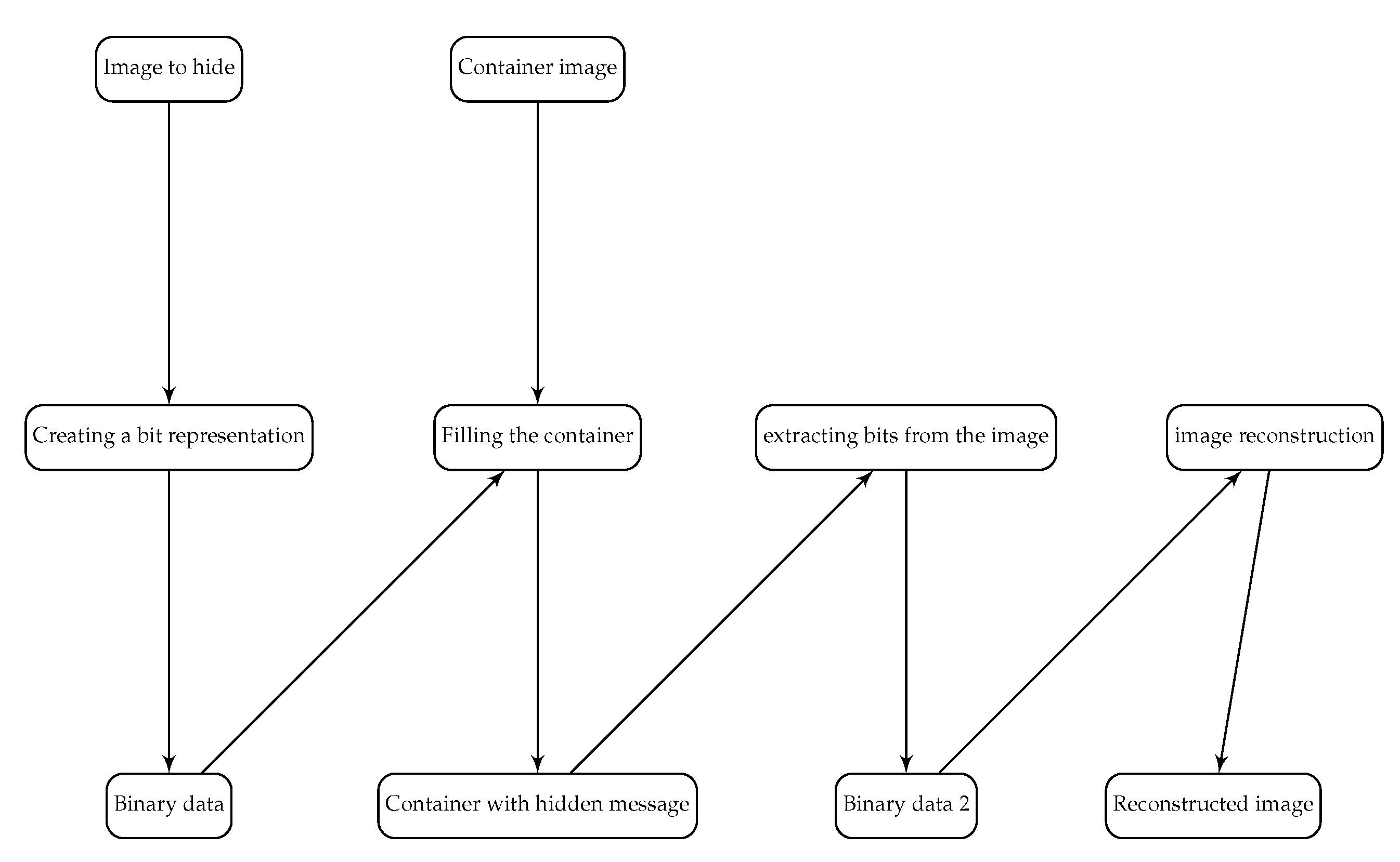
2. Image Steganography

Considering the human eye vision limits one can modify the shades of colors in the picture obtaining the same appearance of the pictures. And this is basically the only reason why we can use steganographic techniques in images.
Computers 09 00038 i001

2.1. Digital Representation of the Image

A digital image can be simply represented by binary numbers of pixel colour saturation in the relevant system. Greyscale image pixels are represented by single Bytes that take decimal values from 0 to 255. In binary format from 00000001 to 11111111. Sample change 01101011 01101010 would not be noticeable to the human eye and in that way we could exploit that shortcoming of a human eye to hide data. R G B image pixels are represented by triples of Bytes, which take decimal values from 0 to 255. For example, white color in decimal form is represented by ( 255 , 255 , 255 ) and in binary form by ( 11111111 , 11111111 , 11111111 ) . Data in digital systems are often shown in hexadecimal form for reading convenience. The white color is ( F F , F F , F F ) where F is the letter of the hexadecimal system alphabet to which a decimal value of 15 is assigned.

2.2. Basic LSB Technique

There are plenty techniques exploiting the limitations of the human eye while looking at the computer image-one of them is using the least significant bit (LSB) method [23,24]. To mask the presence of information transformations are often used-see Reference [17,25]. The LSB method consists in modifying the least significant bit of pixel bytes-the change of which is invisible due to human sight limitations. Let us move on to the demonstration of the use of the technique in an R G B form of image. We want to the letter B in pixel bytes with the following representation.
11101111 11110111 11111011 11111101
11111110 11101111 11110111 11101110
The capital letter B in the ASCII array has the decimal value 65-in binary form it is 01000001. Each decimal value of the ASCII module is written in one Byte, so we complete the received binary value getting 01000001. In this form we can start hiding data.
1110111 0 1111011 1 1111101 0 1111110 0
1111111 0 1110111 0 1111011 0 1110111 1
The expected number of changes we make at the end of the random data is about 50 percent.
The LSB method can be detected by statistical analysis of the typical occurrence of values 1 and 0 at the end of Bytes. Hence, steganographic keys are used to protect information in stego carrier. In doing so embedding an image into a cover picture may can not be noticed to the human eye and, what is more, resistant to statistical tests (like chi-square test) and not to be discovered by an unauthorised person.

2.3. Limitations on the Use of Image Steganography

It is clear that the use of image steganography is detectable in one hundred percent if the attacker has a cover with the same resolution as the stego-carrier. What is attempted to achieve in image steganography is to embed information in such a way that its presence cannot be detected in a stego carrier. This means that the statistics of pixel values in the image do not deviate from the typical ones. One method of such verification is the Chi square test. Our algorithm has successfully passed the test on the examined images, however, statistical tests are not enough to verify effective data embedding. Visualizations based on the last beat of the Pixel Bytes allow to discover a visual trace of the hidden message. An exemplary result of such visualization is presented in Figure 5. It is clear that by embedding a message only in a specific area of the cover, you can see a sign of this data. To avoid this, you can spread the data evenly over the entire image, or use higher bytes to hide the higher bits of Bytes-using the limitations of R G B recognition by the human eye. Of course, in the context of images, the basis for the use of steganography is the application of changes in pixel shades that are not recorded by the human eye. The human eye is only able to recognize from 30 to 50 shades of grey out of 255. The sensitivity of the human eye to color shades varies-see Reference [26]. The human eye can only recognize about 10 million different colors. For example, using R G B , 24 bits per pixel, we have 16,777,216 colors available. This is a huge field for image steganography. Another basic limitation to the use of steganography is interference resulting from scaling, rotation of images. The use of steganography directly with the whole spectrum of colour shades is completely immune to error detection. Because changing one bit leads to a different hue that belongs to a domain. The solution to this problem is to use numeric codes in which the bytes of the message are converted to code words. The main assumption is to get such a set of hue representatives that Hamming’s minimum distance is as large as possible. The minimum distance is simply the smallest Hamming distance (the number of differences on individual bits) among all code word pairs representing pixels. It is well known that when considering the minimal Hamming distance of a set of code words ( C ) representing pixels-denoting by d ( C ) . You can recognize the [ d ( C ) 1 ] errors, and and fix [ d ( C ) 1 ] 2 errors. The longer the code words the longer the distance can be, the limitation is of course the number of bits available in the cover. By notation [x], we denote a feature of a number (its integer part).
To show the limit of use of the least significant bits of R G B bytes, we performed an additional test. We perform an experiment to replace selected bits of R G B bytes with zero values. The effect can be observed in Figure 1, Figure 2 and Figure 3, for R, G and B, respectively.
Using the LSB method, it is very easy to destroy a message, simply by resetting the last bits of the message. So it is basically the weakest steganographic technique in images. We used this technique by its simplicity to present our new steganographic key.

3. Stegoanalysis

There is a number of Stegoanalisys techniques which of course are developed along with the evolution of new steganography methods. An interesting review can be found in References [27,28,29]. We can list the various options: Stego-only attack, Known-cover attack, Known-message attack, Chosen-steganography attack, Chosen-message attack, Known-steganography attack, Statistical analysis, Structural analysis and Signature analysis. In order to study the description of these techniques the reader can consult [27,28,29] and. One of the most popular stegoanalisys techniques is chi-square attack [13], it is a simple and well-known method to test the security system against the attacks-see Section 3.2. The method is based on the analysis of the frequency of occurrence of colour saturation in pairs and detects summary disturbances associated with this distribution. An interesting, simple attack to discover the existence of embedded information is LSB enhancement. The method is described in Section 3.1. Let us present a description of selected stegoanalisys techniques, two of which we implemented for the purpose of the work.

3.1. Stegoanalisys-LSB Enhancement Attack

The technique consists of assigning to bytes of a given colour which contain, in the least significant bit, the value 1, value 11111111. If the last bit is zero, we leave the byte unchanged. In this technique, by enhancing the colours of pixels that have non-zero last bits, we visualize a potentially hidden message. Now, allow us to present the technique in a pseudo-code.
The effect of the method can be seen in the Figure 4 and Figure 5. In particular, in Figure 5 we have a demonstration of how the method makes the embedded information visible in the steganographic carrier. Where in Figure 4 we have its operation shown in the picture without the message embedded.

3.2. Stegoanalisys-Chi Square Attack

The test is used to detect a deviation from the expected statistical dependence of frequency, colour pairs in a fixed size of image blocks. Let us move on to a more detailed introduction with an example. We will start by describing the preparation of a series of data from the image for analysis.
One should consider the color saturation in the range <0–255>, where we have in binary form:
0 D E C : 00000000 B I N
1 D E C : 00000001 B I N
2 D E C : 00000010 B I N
255 D E C : 11111111 B I N
Please consider the following colour pairs, the frequencies of which we will calculate.
P A I R S = { ( 0 D E C , 1 D E C ) , ( 2 D E C , 3 D E C ) ( 254 D E C , 255 D E C ) }
Let us calculate an example of the observed and expected value for the selected pair. Considering ( i D E C , j D E C ) , where color i D E C frequency in the block of data is f r e q ( i D E C ) = 50 , and frequency of j D E C is equal f r e q ( j D E C ) = 20 . The expected value for this pair is equal
e x p e c t e d _ v a l u e ( i D E C , j D E C ) = f r e q ( i D E C ) + f r e q ( j D E C ) 2
In our example it is 35.
o b s e r v e d _ v a l u e ( ( i D E C , j D E C ) = | f r e q ( i D E C ) e x p e c t e d _ v a l u e ( i D E C , j D E C ) |
In our example it is 15. So, we get the first pair of values that will feed the Chi square test. It is
( o b s e r v e d _ v a l u e ( ( i D E C , j D E C ) , e x p e c t e d _ v a l u e ( i D E C , j D E C ) ) = ( 15 , 30 )
The rest of the values for the remaining colour saturation pairs are calculated analogously. The test for all pairs is repeated iteratively on a fixed block size, for example, 64 , 128 , 256 Bytes. After calculating 128 pairs for a given block, we calculate p-value for the Chi square test.
χ 2 = ( o b s e r v e d _ v a l u e ( ( i D E C , j D E C ) e x p e c t e d _ v a l u e ( i D E C , j D E C ) ) 2 e x p e c t e d _ v a l u e ( i D E C , j D E C )
χ 2 summarizes the difference between our data and our independence hypothesis. For a test to be valuable, the data must meet the following assumptions.
(1)
independent observations,
(2)
χ 2 distribution,
To find p-value we need two values: χ 2 and the number of the degrees of freedom (df).
d f = ( n u m b _ o f _ r o w s 1 ) ( n u m b _ o f _ c o l s 1 )
In our case n u m b _ o f _ r o w s = 128 , n u m b _ o f _ c o l s = 2 , thus d f = 127 , and p-value can be found in 1 t a i l e d significance test table.
According to Reference [30], when some data like encrypted image is embedded into another image the LSB values of the original data change in a way that the number of these pairs become nearly equal while they differ so much when there is no embedding.

4. Protection against Stegoanalisys

Naturally, with the development of stegoanalisys techniques, there are methods of defense against them, in this section we will focus on the protection against Chi-square and LSB enhancement attacks. In order to protect the embedded information from detection, we cannot allow the cover image to be made available, because the attacker will detect the embedded information regardless of which technique has been used. The second important step, especially against LSB Enhancement, is the equal distribution of messages throughout the stego-carrier (see in Figure 6). Another simple step to make it easier to protect data against detection is to match a cover to the data, for example, by using images with a specific colour saturation spectrum. Greyscale images are a great place to embed data as the shades change gradually between palette entries. An interesting way, computationally absorptive, but minimizing the number of changes in the cover, is to use data blocks and match data to them. The basic step to hide the presence of information is to use pseudo-random distribution of information-for example, using the RC4 algorithm-see Reference [31]. Another technique to protect data against detection is the widely tested LSB substitution method-see References [1,6,7,8,9,10,18]. Another technique worth mentioning is Data Masking-see Reference [32] (Masking changes the illumination in the masked areas) and filtering-see Reference [33]. Minimize the statistical difference between the cover and the image with the message embedded, for example, the frequency of color saturation pairs. This technique protects against a Chi-square attack-see References [18,34,35].
Let us move on to discussing our technique of creating a steganographic key. We’ll start by introducing the necessary theory.

5. Theoretical Background for Indiscernibility in Degree

A theoretical explanation of the topic of rough inclusions can be found in Pawlak et al. [36], Polkowski [21,22,37,38], a very detailed overview is available in Reference [39]. Let us give the basic information needed to define our technique.
Considering the objects o b 1 , o b 2 belonging to the decision system defined as the triple ( U n i v e r s e , A t t r , d e c ) , where U n i v e r s e is a set of objects, A t t r a set of conditional attributes, and d e c a decision attribute. A rough inclusion is defined as follows
μ ( o b 2 , o b 1 , r a d i u s ) | I N D ( o b 1 , o b 2 ) | | A t t r | r a d i u s .
The granulation radius r a d i u s belongs to the set { i | A t t r | , w h e r e i = 0 . , 1 . , , | A t t r | }
I N D ( o b 1 , o b 2 ) = { a A t t r : a ( o b 1 ) = a ( o b 2 ) } ,
The indiscernibility relation is an equivalence relation. r a d i u s -indiscernible mask is calculated as below:
i f μ ( o b 2 , o b 1 , r a d i u s ) | I N D ( o b 1 , o b 2 ) | | A t t r | = r a d i u s , t h e n c o n c e a l i n f o r m a t i o n b i t i n L S B ,
i f μ ( o b 2 , o b 1 , r a d i u s ) | I N D ( o b 1 , o b 2 ) | | A | r a d i u s , t h e n s k i p t h e B y t e .
Example 1.
if we chose the mask of the length 2, like: _ _ _ _ _ 00 _ (two00on the sixth and seventh position of the bites consecutively), chose the radius equal to r = 1 / 2 and put the mask on byte 00110 01 1 we could see that the difference was on one position out of two (00 versus 01)-that is why we would hide a message bit in LSB in that case. If an exemplary byte was 00110 00 1 the radius would be equal to 1 (different from 1 / 2 ) and in that case the byte would be skipped. Similarly for 00110 11 1 and the radius equal to 0 the byte would be skipped.
In our work we used rough inclusion as a steganographic key.

6. Usage of Our Steganographic Key-the Use of Rough Inclusion to Cover Up Information

Let us describe how we use our steganographic key in LSB technique. Considering the set of R G B pixels, p 1 , p 2 , , p k , where each pixel is defined as:
p i = ( p i r e d p i g r e e n p i b l u e ) :
p i r e d = b 1 p i r e d b 2 p i r e d b 3 p i r e d b 4 p i r e d b 5 p i r e d b 6 p i r e d b 7 p i r e d b 8 p i r e d
p i g r e e n = b 1 p i g r e e n b 2 p i g r e e n b 3 p i g r e e n , b 4 p i g r e e n b 5 p i g r e e n b 6 p i g r e e n b 7 p i g r e e n b 8 p i g r e e n
p i b l u e = b 1 p i b l u e b 2 p i b l u e b 3 p i b l u e b 4 p i b l u e b 5 p i b l u e b 6 p i b l u e b 7 p i b l u e b 8 p i b l u e
For example: this color is represented as ( 11111111 00000000 10000000 ) (decimal form is as follows: (255, 0, 128)).
For a given mask m a s k = ( m a s k 1 , m a s k 2 , , m a s k k ) , k < 8 , the bit of information can be hidden in the Byte ( p i c o l o r ) of pixel p i , in case the following condition is fulfilled:
| I N D ( p i c o l o r , m a s k ) | c a r d { m a s k } = r a d i u s
I N D ( p i c o l o r , m a s k ) = { b i t s B y t e : b i t ( p i c o l o r ) = b i t ( m a s k ) } ,
with the assumption that bits of Bytes and mask bits are compared in the same positions in Byte. Note, that the length of a mask must be not greater than 8-we can use maximum seven positions in a Byte to place the mask upon, whereas the last bit is used for encoding the information in case the mask fits.
In case one uses the methodology proposed above-there are 2 7 different mask that can be used (from the length 1 up to the length 7). By means of a given (fixed) mask the bits of a message can be embedded. It was mentioned before that in doing so we obtain a kind of pseudo-randomness because even starting from the beginning in the cover picture not every byte fits to the mask (which means the least significant bit is not changed) and if it fits the mask with a given ratio the least significant bit might be changed but might be also left unchanged. Let us assume again that our original bits are as follows:
00100110 01011011 10101110 11101111
01010100 01111010 10011001 00010111
and the fixed mask is 00 on two penultimate bits with the ratio r = 0.5 . Putting the mask on bytes one can notice that only the second, the fifth and the sixth byte are used for embedding the message and the other ones create random gaps. Let us assume that the message to hide starts with 111 -then after putting the mask and encoding this fragment one obtains:
00100110 0101101 1 10101110 11101111
0101010 1 0111101 1 10011001 00010111
Notice that on the string of eight Bytes only two changes had to be made with respect to the starting string of Bytes:
00100110 01011011 10101110 11101111
0101010 1 0111101 1 10011001 00010111
Even if these two changes can be notices it is not clear which other Bytes were chosen to hide the message.
In our experiments we considered using different masks for R G B colour.

7. Research Experiments

The diagram showing the general outline of the test we have conducted is in Figure 7, a detailed scheme is shown in Figure 8.
We have used the bitmap library.hpp, see Reference [40]. As a stego carrier we used a picture of 3024 by 4032 pixels from Figure 9. So we have a 3024 4032 3 = 36,578,304 least significant bits available in the stego carrier.
Now allow us to present the characteristics of our method using a sample mask, with sample data.
The image we hide in the first experiment is 453 by 500 pixels-see Figure 10, after breaking down into bits we have 5,436,048 bits to hide, including 48 containing the size of the image. If we use mask = 00 or mask = 11 as the last two bits and assume a degree of indiscernibility of 0.5 we get a 6,233,077 empty slots after embedding the image. The mask itself never changes any bit in the stego carrier but with it we have made 2,715,254 changes during image insertion. If we use a 01 or 10 mask we get 4,720,805 indiscernible Bytes with 2,718,786 changes in the stego carrier.
Let us proceed with the third tests for another image to hide from Figure 11. Its size is 500 × 560 pixels so we have 6,720,048 bits to hide also taking into account three Bytes containing the size of the picture. If we use mask = 10 or mask = 01 as the last penultimate two bits and assume a degree of indiscernibility of 0.5 we get a 5,891,420 empty slots after embedding the image. The mask itself never changes any bit in the stego carrier but with it we have made 3,360,889 changes during image insertion.
The fourth test for another image is to hide Figure 12. Its size is 500 × 332 pixels so we have 3,984,048 bits to hide also taking into account three Bytes containing the size of the picture. If we use mask = 10 or mask = 01 as the last penultimate two bits and assume a degree of indiscernibility of 0.5 we get a 3,388,417 empty slots after embedding the image. The mask itself never changes any bit in the stego carrier but with it we have made 1,990,405 changes during image insertion.
In order to hide the image size into the stego carrier we used two first Bytes at the edge. The pixels are in 24 bits R G B format thus numbering Bytes of the pixels as B 1 , B 2 , , B 6 the size of hidden image can be computed as
h = B 1 D E C B 2 D E C + B 3 D E C
w = B 4 D E C B 5 D E C + B 6 D E C
The DEC means that the Bytes are used in decimal form. Thus in a detailed way: 451 = 255 1 + 196 produces 11111111 00000001 11000100 500 = 255 1 + 245 produces 11111111 00000001 11110101 .
Even if the size of the embedded picture is somehow discovered there is a great difficulty to find which Bytes contain the hidden pictures because of indiscernibility mask application. The size of the picture could be alternatively hidden using indiscernibility mask. What is to be know in order to recover the message? One needs to know which indiscernibility mask has been used.
In order to verify the effectiveness of our information embedding method, we performed a Chi-square and LSB enhancement attack test [30] using the algorithms versions described in Section 3.1 and Section 3.2.
Tests of resistance to detection of the use of LSB, with the help of LSB enhancement were carried out on 35 images from the collection [41]—the sample is in the Figure 13.
It turned out that our technique using the LSB matching method, also using the second least significant bit is resistant to Chi-square attack and LSB enhancement (see examples in Figure 13, Figure 14 and Figure 15). However, assuming that we use images with a variety of colours. In case of a small number of colours with a high frequency, the LSB enhancement method easily discovers the use of our key. That is to say, we assume that our technique works when we deal with the distribution of Chi-square colour saturation frequency.
Please proceed to the presentation of sample data feeding the Chi-square test from a 128 byte data block-considering stego-carrier from Figure 9. We assume that we are considering 3000 line of stego-carrier and file with embedded information.
It is for first 128 Bajts. ( R , G , B ) frequency in stego-carrier: in the spectrum [ 0 , 255 ] :
( 1 , 1 , 1 ) , ( 1 , 1 , 1 ) , ( 2 , 2 , 2 ) , ( 3 , 3 , 3 ) , ( 1 , 1 , 1 ) , ( 4 , 1 , 2 ) , ( 1 , 2 , 1 ) , ( 1 , 1 , 1 ) , ( 1 , 2 , 1 ) , ( 5 , 3 , 3 ) , ( 2 , 4 , 4 ) , ( 2 , 3 , 2 ) , ( 2 , 2 , 2 ) , ( 3 , 4 , 2 ) , ( 4 , 5 , 5 ) , ( 2 , 4 , 2 ) , ( 6 , 6 , 6 ) , ( 5 , 5 , 4 ) , ( 7 , 6 , 5 ) , ( 8 , 7 , 7 ) , ( 9 , 8 , 8 ) , ( 1 , 2 , 6 ) , ( 10 , 7 , 7 ) , ( 11 , 9 , 9 ) , ( 3 , 1 , 3 ) , ( 3 , 10 , 3 ) , ( 12 , 11 , 10 ) , ( 2 , 3 , 8 ) , ( 3 , 4 , 9 ) , ( 13 , 8 , 3 ) , ( 14 , 9 , 10 ) , ( 4 , 5 , 11 ) , ( 1 , 1 , 1 ) , ( 15 , 10 , 4 ) , ( 1 , 1 , 1 ) , ( 16 , 3 , 11 ) , ( 1 , 1 , 1 ) , ( 17 , 4 , 12 ) , ( 18 , 12 , 13 ) , ( 4 , 2 , 4 ) , ( 5 , 3 , 5 ) , ( 6 , 13 , 14 ) , ( 4 , 14 , 4 ) , ( 5 , 15 , 5 ) , ( 19 , 16 , 15 ) , ( 7 , 17 , 16 ) , ( 20 , 18 , 17 ) , ( 2 , 2 , 2 ) , ( 2 , 1 , 3 ) , ( 3 , 3 , 4 ) , ( 6 , 19 , 6 ) , ( 3 , 5 , 3 ) , ( 2 , 1 , 1 ) , ( 6 , 4 , 6 ) , ( 7 , 5 , 7 ) , ( 5 , 2 , 2 ) , ( 8 , 20 , 18 ) , ( 8 , 21 , 8 ) , ( 21 , 22 , 19 ) , ( 22 , 11 , 12 ) , ( 9 , 6 , 20 ) , ( 9 , 23 , 9 ) , ( 7 , 5 , 7 ) , ( 4 , 4 , 5 ) , ( 10 , 7 , 10 ) , ( 8 , 6 , 8 ) , ( 6 , 6 , 5 ) , ( 23 , 24 , 21 ) , ( 4 , 7 , 4 ) , ( 24 , 25 , 22 ) , ( 11 , 26 , 11 ) , ( 12 , 27 , 12 ) , ( 10 , 12 , 13 ) , ( 13 , 28 , 13 ) , ( 5 , 8 , 5 ) , ( 9 , 9 , 9 ) , ( 25 , 13 , 6 ) , ( 14 , 29 , 14 ) , ( 6 , 6 , 6 ) , ( 15 , 30 , 15 ) , ( 7 , 7 , 23 ) , ( 16 , 31 , 7 ) , ( 7 , 10 , 6 ) , ( 17 , 32 , 8 ) , ( 18 , 8 , 9 ) , ( 10 , 11 , 1 ) , ( 8 , 12 , 7 ) , ( 11 , 13 , 8 ) , ( 26 , 33 , 10 ) , ( 11 , 9 , 11 ) , ( 27 , 34 , 12 ) , ( 19 , 35 , 10 ) , ( 20 , 36 , 11 ) , ( 28 , 14 , 16 ) , ( 29 , 15 , 17 ) , ( 21 , 37 , 12 ) , ( 30 , 38 , 13 ) , ( 12 , 14 , 9 ) , ( 13 , 15 , 10 ) , ( 22 , 10 , 13 ) , ( 23 , 39 , 14 ) , ( 31 , 40 , 14 ) , ( 24 , 11 , 15 ) , ( 14 , 16 , 11 ) , ( 12 , 16 , 18 ) , ( 25 , 41 , 16 ) , ( 15 , 17 , 2 ) , ( 26 , 42 , 17 ) , ( 16 , 18 , 3 ) , ( 9 , 19 , 12 ) , ( 13 , 43 , 15 ) , ( 27 , 44 , 18 ) , ( 8 , 8 , 24 ) , ( 1 , 1 , 2 ) , ( 9 , 9 , 25 ) , ( 28 , 12 , 19 ) , ( 32 , 17 , 19 ) , ( 33 , 13 , 16 ) , ( 10 , 20 , 13 ) , ( 14 , 18 , 20 ) , ( 2 , 2 , 14 ) , ( 10 , 10 , 26 ) , ( 34 , 19 , 21 ) , ( 15 , 20 , 22 ) , ( 11 , 3 , 7 ) , ( 12 , 11 , 27 ) , ( 35 , 45 , 17 ) , ( 17 , 21 , 14 )
R G B frequency in stego-carrier with embedded data-from Figure 16: in the spectrum [ 0 , 255 ] :
( 1 , 1 , 1 ) , ( 1 , 1 , 1 ) , ( 2 , 2 , 2 ) , ( 3 , 3 , 3 ) , ( 1 , 1 , 1 ) , ( 1 , 1 , 1 ) , ( 2 , 2 , 2 ) , ( 1 , 1 , 1 ) , ( 1 , 1 , 1 ) , ( 3 , 3 , 3 ) , ( 4 , 4 , 4 ) , ( 2 , 2 , 2 ) , ( 2 , 2 , 2 ) , ( 4 , 4 , 4 ) , ( 5 , 5 , 5 ) , ( 2 , 2 , 2 ) , ( 6 , 6 , 6 ) , ( 5 , 5 , 5 ) , ( 6 , 6 , 6 ) , ( 7 , 7 , 7 ) , ( 8 , 8 , 8 ) , ( 2 , 2 , 2 ) , ( 7 , 7 , 7 ) , ( 9 , 9 , 9 ) , ( 3 , 3 , 3 ) , ( 3 , 3 , 3 ) , ( 10 , 10 , 10 ) , ( 3 , 3 , 3 ) , ( 4 , 4 , 4 ) , ( 8 , 8 , 8 ) , ( 9 , 9 , 9 ) , ( 5 , 5 , 5 ) , ( 1 , 1 , 1 ) , ( 10 , 10 , 10 ) , ( 1 , 1 , 1 ) , ( 11 , 11 , 11 ) , ( 1 , 1 , 1 ) , ( 12 , 12 , 12 ) , ( 13 , 13 , 13 ) , ( 4 , 4 , 4 ) , ( 5 , 5 , 5 ) , ( 14 , 14 , 14 ) , ( 4 , 4 , 4 ) , ( 5 , 5 , 5 ) , ( 15 , 15 , 15 ) , ( 16 , 16 , 16 ) , ( 17 , 17 , 17 ) , ( 2 , 2 , 2 ) , ( 1 , 1 , 1 ) , ( 3 , 3 , 3 ) , ( 6 , 6 , 6 ) , ( 3 , 3 , 3 ) , ( 1 , 1 , 1 ) , ( 6 , 6 , 6 ) , ( 7 , 7 , 7 ) , ( 2 , 2 , 2 ) , ( 18 , 18 , 18 ) , ( 8 , 8 , 8 ) , ( 19 , 19 , 19 ) , ( 11 , 11 , 11 ) , ( 20 , 20 , 20 ) , ( 9 , 9 , 9 ) , ( 7 , 7 , 7 ) , ( 4 , 4 , 4 ) , ( 10 , 10 , 10 ) , ( 8 , 8 , 8 ) , ( 6 , 6 , 6 ) , ( 21 , 21 , 21 ) , ( 4 , 4 , 4 ) , ( 22 , 22 , 22 ) , ( 11 , 11 , 11 ) , ( 12 , 12 , 12 ) , ( 12 , 12 , 12 ) , ( 13 , 13 , 13 ) , ( 5 , 5 , 5 ) , ( 9 , 9 , 9 ) , ( 13 , 13 , 13 ) , ( 14 , 14 , 14 ) , ( 6 , 6 , 6 ) , ( 15 , 15 , 15 ) , ( 7 , 7 , 23 ) , ( 16 , 16 , 7 ) , ( 7 , 7 , 2 ) , ( 17 , 17 , 8 ) , ( 18 , 18 , 9 ) , ( 10 , 10 , 5 ) , ( 8 , 8 , 3 ) , ( 11 , 11 , 6 ) , ( 23 , 23 , 10 ) , ( 24 , 24 , 11 ) , ( 25 , 25 , 12 ) , ( 19 , 19 , 10 ) , ( 20 , 20 , 11 ) , ( 14 , 14 , 16 ) , ( 15 , 15 , 17 ) , ( 21 , 21 , 12 ) , ( 26 , 26 , 13 ) , ( 12 , 12 , 7 ) , ( 13 , 13 , 8 ) , ( 22 , 22 , 13 ) , ( 23 , 23 , 14 ) , ( 27 , 27 , 14 ) , ( 24 , 24 , 15 ) , ( 14 , 14 , 9 ) , ( 16 , 16 , 18 ) , ( 25 , 25 , 16 ) , ( 15 , 15 , 10 ) , ( 26 , 26 , 17 ) , ( 16 , 16 , 11 ) , ( 9 , 9 , 4 ) , ( 28 , 28 , 15 ) , ( 27 , 27 , 18 ) , ( 8 , 8 , 24 ) , ( 1 , 1 , 3 ) , ( 9 , 9 , 25 ) , ( 28 , 28 , 19 ) , ( 17 , 17 , 19 ) , ( 29 , 29 , 16 ) , ( 10 , 10 , 5 ) , ( 18 , 18 , 20 ) , ( 2 , 2 , 7 ) , ( 10 , 10 , 26 ) , ( 19 , 19 , 21 ) , ( 20 , 20 , 22 ) , ( 3 , 3 , 14 ) , ( 11 , 11 , 27 ) , ( 30 , 30 , 17 ) , ( 17 , 17 , 12 )
Based on above data R pairs for stego-carrier are as follows, C h i s q u a r e = 32.99
( 0 , 0 ) , ( 0 , 0 ) , ( 0 , 0 ) , ( 0 , 0 ) , ( 0 , 0 ) , ( 0 , 0 ) , ( 0 , 0 ) , ( 0 , 0 ) , ( 0 , 0 ) , ( 0 , 0 ) , ( 0 , 0 ) , ( 0 , 0 ) , ( 0 , 0 ) , ( 0 , 0 ) , ( 0 , 0 ) , ( 0 , 0 ) , ( 0 , 0 ) , ( 0 , 0 ) , ( 0 , 0 ) , ( 0 , 0 ) , ( 0 , 0 ) , ( 0 , 0 ) , ( 0 , 0 ) , ( 0 , 0 ) , ( 0 , 0 ) , ( 0 , 0 ) , ( 0 , 0 ) , ( 0 , 0 ) , ( 0 , 0 ) , ( 0 , 0 ) , ( 0 , 0 ) , ( 0 , 0 ) , ( 0 , 0 ) , ( 0 , 0 ) , ( 0 , 0 ) , ( 0 , 0 ) , ( 0 , 0 ) , ( 0 , 0 ) , ( 0 , 0 ) , ( 0 , 0 ) , ( 0 , 0 ) , ( 0 , 0 ) , ( 0 , 0 ) , ( 0 , 0 ) , ( 0 , 0 ) , ( 0 , 0 ) , ( 0 , 0 ) , ( 0 , 0 ) , ( 0 , 0 ) , ( 0 , 0 ) , ( 0 , 0 ) , ( 0 , 0 ) , ( 0 , 0 ) , ( 0 , 0 ) , ( 0 , 0 ) , ( 0 , 0 ) , ( 0 , 0 ) , ( 0 , 0 ) , ( 0 , 0 ) , ( 0 , 0 ) , ( 0 , 0 ) , ( 0 , 0 ) , ( 0 , 0 ) , ( 0 , 0 ) , ( 0 , 0 ) , ( 0 , 0 ) , ( 0 , 0 ) , ( 0 , 0 ) , ( 0 , 0 ) , ( 0 , 0 ) , ( 0 , 0 ) , ( 0 , 0 ) , ( 0 , 0 ) , ( 0 , 0 ) , ( 0 , 0 ) , ( 0 , 0 ) , ( 0 , 0 ) , ( 0 , 0 ) , ( 0 , 0 ) , ( 0 , 0 ) , ( 0 , 0 ) , ( 0 , 0 ) , ( 0 , 0 ) , ( 0 , 0 ) , ( 0 , 0 ) , ( 0 , 0 ) , ( 0 , 0 ) , ( 0 , 0 ) , ( 0 , 0 ) , ( 0 , 0 ) , ( 0 , 0 ) , ( 0 , 0 ) , ( 0 , 0 ) , ( 0 , 0 ) , ( 0 , 0 ) , ( 0 , 0 ) , ( 0 , 0 ) , ( 0 , 0 ) , ( 0 , 0 ) , ( 0 , 0 ) , ( 1 , 1 ) , ( 3 , 7 ) , ( 5 , 22 ) , ( 10 , 25 ) , ( 5 , 7 ) , ( 1 , 1 ) , ( 0 , 0 ) , ( 0 , 0 ) , ( 0 , 0 ) , ( 0 , 0 ) , ( 0 , 0 ) , ( 0 , 0 ) , ( 0 , 0 ) , ( 0 , 0 ) , ( 0 , 0 ) , ( 0 , 0 ) , ( 0 , 0 ) , ( 0 , 0 ) , ( 0 , 0 ) , ( 0 , 0 ) , ( 0 , 0 ) , ( 0 , 0 ) , ( 0 , 0 ) , ( 0 , 0 ) , ( 0 , 0 ) , ( 0 , 0 ) , ( 0 , 0 ) , ( 0 , 0 )
In case of embedded data, C h i s q u a r e = 33.71
( 0 , 0 ) , ( 0 , 0 ) , ( 0 , 0 ) , ( 0 , 0 ) , ( 0 , 0 ) , ( 0 , 0 ) , ( 0 , 0 ) , ( 0 , 0 ) , ( 0 , 0 ) , ( 0 , 0 ) , ( 0 , 0 ) , ( 0 , 0 ) , ( 0 , 0 ) , ( 0 , 0 ) , ( 0 , 0 ) , ( 0 , 0 ) , ( 0 , 0 ) , ( 0 , 0 ) , ( 0 , 0 ) , ( 0 , 0 ) , ( 0 , 0 ) , ( 0 , 0 ) , ( 0 , 0 ) , ( 0 , 0 ) , ( 0 , 0 ) , ( 0 , 0 ) , ( 0 , 0 ) , ( 0 , 0 ) , ( 0 , 0 ) , ( 0 , 0 ) , ( 0 , 0 ) , ( 0 , 0 ) , ( 0 , 0 ) , ( 0 , 0 ) , ( 0 , 0 ) , ( 0 , 0 ) , ( 0 , 0 ) , ( 0 , 0 ) , ( 0 , 0 ) , ( 0 , 0 ) , ( 0 , 0 ) , ( 0 , 0 ) , ( 0 , 0 ) , ( 0 , 0 ) , ( 0 , 0 ) , ( 0 , 0 ) , ( 0 , 0 ) , ( 0 , 0 ) , ( 0 , 0 ) , ( 0 , 0 ) , ( 0 , 0 ) , ( 0 , 0 ) , ( 0 , 0 ) , ( 0 , 0 ) , ( 0 , 0 ) , ( 0 , 0 ) , ( 0 , 0 ) , ( 0 , 0 ) , ( 0 , 0 ) , ( 0 , 0 ) , ( 0 , 0 ) , ( 0 , 0 ) , ( 0 , 0 ) , ( 0 , 0 ) , ( 0 , 0 ) , ( 0 , 0 ) , ( 0 , 0 ) , ( 0 , 0 ) , ( 0 , 0 ) , ( 0 , 0 ) , ( 0 , 0 ) , ( 0 , 0 ) , ( 0 , 0 ) , ( 0 , 0 ) , ( 0 , 0 ) , ( 0 , 0 ) , ( 0 , 0 ) , ( 0 , 0 ) , ( 0 , 0 ) , ( 0 , 0 ) , ( 0 , 0 ) , ( 0 , 0 ) , ( 0 , 0 ) , ( 0 , 0 ) , ( 0 , 0 ) , ( 0 , 0 ) , ( 0 , 0 ) , ( 0 , 0 ) , ( 0 , 0 ) , ( 0 , 0 ) , ( 0 , 0 ) , ( 0 , 0 ) , ( 0 , 0 ) , ( 0 , 0 ) , ( 0 , 0 ) , ( 0 , 0 ) , ( 0 , 0 ) , ( 0 , 0 ) , ( 0 , 0 ) , ( 0 , 0 ) , ( 0 , 1 ) , ( 3 , 7 ) , ( 5 , 22 ) , ( 5 , 25 ) , ( 4 , 7 ) , ( 1 , 1 ) , ( 0 , 0 ) , ( 0 , 0 ) , ( 0 , 0 ) , ( 0 , 0 ) , ( 0 , 0 ) , ( 0 , 0 ) , ( 0 , 0 ) , ( 0 , 0 ) , ( 0 , 0 ) , ( 0 , 0 ) , ( 0 , 0 ) , ( 0 , 0 ) , ( 0 , 0 ) , ( 0 , 0 ) , ( 0 , 0 ) , ( 0 , 0 ) , ( 0 , 0 ) , ( 0 , 0 ) , ( 0 , 0 ) , ( 0 , 0 ) , ( 0 , 0 ) , ( 0 , 0 )
Based on above data G pairs ( o b s e r v e d , e x p e c t e d ) for stego-carrier are as follows, C h i s q u a r e = 15.42 .
( 0 , 0 ) , ( 0 , 0 ) , ( 0 , 0 ) , ( 0 , 0 ) , ( 0 , 0 ) , ( 0 , 0 ) , ( 0 , 0 ) , ( 0 , 0 ) , ( 0 , 0 ) , ( 0 , 0 ) , ( 0 , 0 ) , ( 0 , 0 ) , ( 0 , 0 ) , ( 0 , 0 ) , ( 0 , 0 ) , ( 0 , 0 ) , ( 0 , 0 ) , ( 0 , 0 ) , ( 0 , 0 ) , ( 0 , 0 ) , ( 0 , 0 ) , ( 0 , 0 ) , ( 0 , 0 ) , ( 0 , 0 ) , ( 0 , 0 ) , ( 0 , 0 ) , ( 0 , 0 ) , ( 0 , 0 ) , ( 0 , 0 ) , ( 0 , 0 ) , ( 0 , 0 ) , ( 0 , 0 ) , ( 0 , 0 ) , ( 0 , 0 ) , ( 0 , 0 ) , ( 0 , 0 ) , ( 0 , 0 ) , ( 0 , 0 ) , ( 0 , 0 ) , ( 0 , 0 ) , ( 0 , 0 ) , ( 0 , 0 ) , ( 0 , 0 ) , ( 0 , 0 ) , ( 0 , 0 ) , ( 0 , 0 ) , ( 0 , 0 ) , ( 0 , 0 ) , ( 0 , 0 ) , ( 0 , 0 ) , ( 0 , 0 ) , ( 0 , 0 ) , ( 0 , 0 ) , ( 0 , 0 ) , ( 0 , 0 ) , ( 0 , 0 ) , ( 0 , 0 ) , ( 0 , 0 ) , ( 0 , 0 ) , ( 0 , 0 ) , ( 0 , 0 ) , ( 0 , 0 ) , ( 0 , 0 ) , ( 0 , 0 ) , ( 0 , 0 ) , ( 0 , 0 ) , ( 0 , 0 ) , ( 0 , 0 ) , ( 0 , 0 ) , ( 0 , 0 ) , ( 0 , 0 ) , ( 0 , 0 ) , ( 0 , 0 ) , ( 0 , 0 ) , ( 0 , 0 ) , ( 0 , 0 ) , ( 0 , 0 ) , ( 0 , 0 ) , ( 0 , 0 ) , ( 0 , 0 ) , ( 0 , 0 ) , ( 0 , 0 ) , ( 0 , 0 ) , ( 0 , 0 ) , ( 0 , 0 ) , ( 0 , 0 ) , ( 0 , 0 ) , ( 0 , 0 ) , ( 0 , 0 ) , ( 0 , 0 ) , ( 0 , 0 ) , ( 0 , 0 ) , ( 0 , 0 ) , ( 0 , 0 ) , ( 0 , 0 ) , ( 0 , 0 ) , ( 0 , 0 ) , ( 0 , 0 ) , ( 1 , 2 ) , ( 8 , 13 ) , ( 16 , 29 ) , ( 5 , 15 ) , ( 1 , 2 ) , ( 0 , 0 ) , ( 0 , 0 ) , ( 0 , 0 ) , ( 0 , 0 ) , ( 0 , 0 ) , ( 0 , 0 ) , ( 0 , 0 ) , ( 0 , 0 ) , ( 0 , 0 ) , ( 0 , 0 ) , ( 0 , 0 ) , ( 0 , 0 ) , ( 0 , 0 ) , ( 0 , 0 ) , ( 0 , 0 ) , ( 0 , 0 ) , ( 0 , 0 ) ( 0 , 0 ) , ( 0 , 0 ) , ( 0 , 0 ) , ( 0 , 0 ) , ( 0 , 0 ) , ( 0 , 0 ) , ( 0 , 0 ) , ( 0 , 0 )
In case of embedded data, C h i s q u a r e = 42.39
( 0 , 0 ) , ( 0 , 0 ) , ( 0 , 0 ) , ( 0 , 0 ) , ( 0 , 0 ) , ( 0 , 0 ) , ( 0 , 0 ) , ( 0 , 0 ) , ( 0 , 0 ) , ( 0 , 0 ) , ( 0 , 0 ) , ( 0 , 0 ) , ( 0 , 0 ) , ( 0 , 0 ) , ( 0 , 0 ) , ( 0 , 0 ) , ( 0 , 0 ) , ( 0 , 0 ) , ( 0 , 0 ) , ( 0 , 0 ) , ( 0 , 0 ) , ( 0 , 0 ) , ( 0 , 0 ) , ( 0 , 0 ) , ( 0 , 0 ) , ( 0 , 0 ) , ( 0 , 0 ) , ( 0 , 0 ) , ( 0 , 0 ) , ( 0 , 0 ) , ( 0 , 0 ) , ( 0 , 0 ) , ( 0 , 0 ) , ( 0 , 0 ) , ( 0 , 0 ) , ( 0 , 0 ) , ( 0 , 0 ) , ( 0 , 0 ) , ( 0 , 0 ) , ( 0 , 0 ) , ( 0 , 0 ) , ( 0 , 0 ) , ( 0 , 0 ) , ( 0 , 0 ) , ( 0 , 0 ) , ( 0 , 0 ) , ( 0 , 0 ) , ( 0 , 0 ) , ( 0 , 0 ) , ( 0 , 0 ) , ( 0 , 0 ) , ( 0 , 0 ) , ( 0 , 0 ) , ( 0 , 0 ) , ( 0 , 0 ) , ( 0 , 0 ) , ( 0 , 0 ) , ( 0 , 0 ) , ( 0 , 0 ) , ( 0 , 0 ) , ( 0 , 0 ) , ( 0 , 0 ) , ( 0 , 0 ) , ( 0 , 0 ) , ( 0 , 0 ) , ( 0 , 0 ) , ( 0 , 0 ) , ( 0 , 0 ) , ( 0 , 0 ) , ( 0 , 0 ) , ( 0 , 0 ) , ( 0 , 0 ) , ( 0 , 0 ) , ( 0 , 0 ) , ( 0 , 0 ) , ( 0 , 0 ) , ( 0 , 0 ) , ( 0 , 0 ) , ( 0 , 0 ) , ( 0 , 0 ) , ( 0 , 0 ) , ( 0 , 0 ) , ( 0 , 0 ) , ( 0 , 0 ) , ( 0 , 0 ) , ( 0 , 0 ) , ( 0 , 0 ) , ( 0 , 0 ) , ( 0 , 0 ) , ( 0 , 0 ) , ( 0 , 0 ) , ( 0 , 0 ) , ( 0 , 0 ) , ( 0 , 0 ) , ( 0 , 0 ) , ( 0 , 0 ) , ( 0 , 0 ) , ( 0 , 0 ) , ( 1 , 2 ) , ( 3 , 13 ) , ( 1 , 29 ) , ( 5 , 15 ) , ( 1 , 2 ) , ( 1 , 0 ) , ( 0 , 0 ) , ( 0 , 0 ) , ( 0 , 0 ) , ( 0 , 0 ) , ( 0 , 0 ) , ( 0 , 0 ) , ( 0 , 0 ) , ( 0 , 0 ) , ( 0 , 0 ) , ( 0 , 0 ) , ( 0 , 0 ) , ( 0 , 0 ) , ( 0 , 0 ) , ( 0 , 0 ) , ( 0 , 0 ) , ( 0 , 0 ) , ( 0 , 0 ) , ( 0 , 0 ) , ( 0 , 0 ) , ( 0 , 0 ) , ( 0 , 0 ) , ( 0 , 0 ) , ( 0 , 0 ) , ( 0 , 0 )
Based on above data B pairs ( o b s e r v e d , e x p e c t e d ) for stego-carrier are as follows, C h i s q u a r e = 42.32 .
( 0 , 0 ) , ( 0 , 0 ) , ( 0 , 0 ) , ( 0 , 0 ) , ( 0 , 0 ) , ( 0 , 0 ) , ( 0 , 0 ) , ( 0 , 0 ) , ( 0 , 0 ) , ( 0 , 0 ) , ( 0 , 0 ) , ( 0 , 0 ) , ( 0 , 0 ) , ( 0 , 0 ) , ( 0 , 0 ) , ( 0 , 0 ) , ( 0 , 0 ) , ( 0 , 0 ) , ( 0 , 0 ) , ( 0 , 0 ) , ( 0 , 0 ) , ( 0 , 0 ) , ( 0 , 0 ) , ( 0 , 0 ) , ( 0 , 0 ) , ( 0 , 0 ) , ( 0 , 0 ) , ( 0 , 0 ) , ( 0 , 0 ) , ( 0 , 0 ) , ( 0 , 0 ) , ( 0 , 0 ) , ( 0 , 0 ) , ( 0 , 0 ) , ( 0 , 0 ) , ( 0 , 0 ) , ( 0 , 0 ) , ( 0 , 0 ) , ( 0 , 0 ) , ( 0 , 0 ) , ( 0 , 0 ) , ( 0 , 0 ) , ( 0 , 0 ) , ( 0 , 0 ) , ( 0 , 0 ) , ( 0 , 0 ) , ( 0 , 0 ) , ( 0 , 0 ) , ( 0 , 0 ) , ( 0 , 0 ) , ( 0 , 0 ) , ( 0 , 0 ) , ( 0 , 0 ) , ( 0 , 0 ) , ( 0 , 0 ) , ( 0 , 0 ) , ( 0 , 0 ) , ( 0 , 0 ) , ( 0 , 0 ) , ( 0 , 0 ) , ( 0 , 0 ) , ( 0 , 0 ) , ( 0 , 0 ) , ( 0 , 0 ) , ( 0 , 0 ) , ( 0 , 0 ) , ( 0 , 0 ) , ( 0 , 0 ) , ( 0 , 0 ) , ( 0 , 0 ) , ( 0 , 0 ) , ( 0 , 0 ) , ( 0 , 0 ) , ( 0 , 0 ) , ( 0 , 0 ) , ( 0 , 0 ) , ( 0 , 0 ) , ( 0 , 0 ) , ( 0 , 0 ) , ( 0 , 0 ) , ( 0 , 0 ) , ( 0 , 0 ) , ( 0 , 0 ) , ( 0 , 0 ) , ( 0 , 0 ) , ( 0 , 0 ) , ( 0 , 0 ) , ( 0 , 0 ) , ( 0 , 0 ) , ( 0 , 0 ) , ( 0 , 0 ) , ( 0 , 0 ) , ( 0 , 0 ) , ( 0 , 0 ) , ( 0 , 0 ) , ( 1 , 0 ) , ( 6 , 8 ) , ( 1 , 18 ) , ( 2 , 24 ) , ( 4 , 10 ) , ( 0 , 2 ) , ( 0 , 0 ) , ( 0 , 0 ) , ( 0 , 0 ) , ( 0 , 0 ) , ( 0 , 0 ) , ( 0 , 0 ) , ( 0 , 0 ) , ( 0 , 0 ) , ( 0 , 0 ) , ( 0 , 0 ) , ( 0 , 0 ) , ( 0 , 0 ) , ( 0 , 0 ) , ( 0 , 0 ) , ( 0 , 0 ) , ( 0 , 0 ) , ( 0 , 0 ) , ( 0 , 0 ) , ( 0 , 0 ) , ( 0 , 0 ) , ( 0 , 0 ) , ( 0 , 0 ) , ( 0 , 0 ) , ( 0 , 0 ) , ( 0 , 0 ) , ( 0 , 0 ) , ( 0 , 0 )
In case of embedded data, C h i s q u a r e = 43.45 .
( 0 , 0 ) , ( 0 , 0 ) , ( 0 , 0 ) , ( 0 , 0 ) , ( 0 , 0 ) , ( 0 , 0 ) , ( 0 , 0 ) , ( 0 , 0 ) , ( 0 , 0 ) , ( 0 , 0 ) , ( 0 , 0 ) , ( 0 , 0 ) , ( 0 , 0 ) , ( 0 , 0 ) , ( 0 , 0 ) , ( 0 , 0 ) , ( 0 , 0 ) , ( 0 , 0 ) , ( 0 , 0 ) , ( 0 , 0 ) , ( 0 , 0 ) , ( 0 , 0 ) , ( 0 , 0 ) , ( 0 , 0 ) , ( 0 , 0 ) , ( 0 , 0 ) , ( 0 , 0 ) , ( 0 , 0 ) , ( 0 , 0 ) , ( 0 , 0 ) , ( 0 , 0 ) , ( 0 , 0 ) , ( 0 , 0 ) , ( 0 , 0 ) , ( 0 , 0 ) , ( 0 , 0 ) , ( 0 , 0 ) , ( 0 , 0 ) , ( 0 , 0 ) , ( 0 , 0 ) , ( 0 , 0 ) , ( 0 , 0 ) , ( 0 , 0 ) , ( 0 , 0 ) , ( 0 , 0 ) , ( 0 , 0 ) , ( 0 , 0 ) , ( 0 , 0 ) , ( 0 , 0 ) , ( 0 , 0 ) , ( 0 , 0 ) , ( 0 , 0 ) , ( 0 , 0 ) , ( 0 , 0 ) , ( 0 , 0 ) , ( 0 , 0 ) , ( 0 , 0 ) , ( 0 , 0 ) , ( 0 , 0 ) , ( 0 , 0 ) , ( 0 , 0 ) , ( 0 , 0 ) , ( 0 , 0 ) , ( 0 , 0 ) , ( 0 , 0 ) , ( 0 , 0 ) , ( 0 , 0 ) , ( 0 , 0 ) , ( 0 , 0 ) , ( 0 , 0 ) , ( 0 , 0 ) , ( 0 , 0 ) , ( 0 , 0 ) , ( 0 , 0 ) , ( 0 , 0 ) , ( 0 , 0 ) , ( 0 , 0 ) , ( 0 , 0 ) , ( 0 , 0 ) , ( 0 , 0 ) , ( 0 , 0 ) , ( 0 , 0 ) , ( 0 , 0 ) , ( 0 , 0 ) , ( 0 , 0 ) , ( 0 , 0 ) , ( 0 , 0 ) , ( 0 , 0 ) , ( 0 , 0 ) , ( 0 , 0 ) , ( 0 , 0 ) , ( 0 , 0 ) , ( 0 , 0 ) , ( 0 , 0 ) , ( 0 , 0 ) , ( 0 , 0 ) , ( 3 , 8 ) , ( 1 , 18 ) , ( 2 , 24 ) , ( 4 , 10 ) , ( 1 , 2 ) , ( 0 , 0 ) , ( 0 , 0 ) , ( 0 , 0 ) , ( 0 , 0 ) , ( 0 , 0 ) , ( 0 , 0 ) , ( 0 , 0 ) , ( 0 , 0 ) , ( 0 , 0 ) , ( 0 , 0 ) , ( 0 , 0 ) , ( 0 , 0 ) , ( 0 , 0 ) , ( 0 , 0 ) , ( 0 , 0 ) , ( 0 , 0 ) , ( 0 , 0 ) , ( 0 , 0 ) , ( 0 , 0 ) , ( 0 , 0 ) , ( 0 , 0 ) , ( 0 , 0 ) , ( 0 , 0 ) , ( 0 , 0 ) , ( 0 , 0 ) , ( 0 , 0 ) , ( 0 , 0 )
For all data blocks in the container and image with the message embedded, c h i s q u a r e < 50 , and p-value = 1, its proof that there is no significant difference-with significance 0.05 . Message can be detected in case the Chi-square is larger than 154.

8. Conclusions

In this article we have applied rough inclusions to form the steganographic key. The use of rough inclusions and an additional mask to indicate the bytes in which the information is embedded allows the data to be hidden in a semi-random way, which-with evenly distributed in the stego carrier-hides their presence. We have conducted experiments which present our technique and its features. For demonstration purposes we used selected masks and indiscernibility levels. Using our method when embedding information a large number of random gaps are created in which the data is not hidden. For the simplicity of presentation we chose the LSB method as a base to demonstrate our key. We used a simple LSB matching technique to hide embedded data by using our steganographic key. The hiding method proved to be resistant to Chi Square attack and LSB enhancement-assuming that the images we use contain the entire color palette. In images where we have a small number of distinguishable colors, it is difficult to hide the presence of the contained information against an LSB enhancement attack. Another problem is the use of an indiscernible mask with a certain tolerance, if we apply the LSB enhancement tolerance it can expose the presence of the message. From our preliminary results we can see that precise indication of the degree of indiscernibility works effectively.
Another research topic will be the use of methods to protect the embedded information from damage, among other things, we plan to use selected codes to increase the Hamming distance of the embedded data bytes. We treat our results as preliminary, in future works we plan to test the whole spectrum of possible masks and techniques of hiding the presence embedded with our information key. This work is the starting point for a series of studies on the application of out granular computing tools in steganography.

Author Contributions

Conceptualization, P.A.; Methodology, P.A. and A.K.-M.; Software, P.A. and A.K.-M.; Validation, P.A.; Formal Analysis, P.A.; Investigation, P.A.; Resources, P.A. and A.K.-M.; Writing—Original Draft Preparation, P.A. and A.K.-M.; Writing—Review and Editing, P.A. and A.K.-M.; Visualization, P.A.; Project Administration, P.A. Funding Acquisition, P.A. and A.K.-M. All authors have read and agreed to the published version of the manuscript.

Funding

This work has been fully supported by the grant from Ministry of Science and Higher Education of the Republic of Poland under the project number 23.610.007-300.

Acknowledgments

The research has been supported by grant 23.610.007-000 from Ministry of Science and Higher Education of the Republic of Poland.

Conflicts of Interest

The authors declare no conflict of interest. The funders had no role in the design of the study; in the collection, analyses, or interpretation of data; in the writing of the manuscript, or in the decision to publish the results.

References

  1. Zakaria, A.A.; Hussain, M.; Wahab, A.W.A.; Idris, M.Y.I.; Abdullah, N.A.; Jung, K.-H. High-Capacity Image Steganography with Minimum Modified Bits Based on Data Mapping and LSB Substitution. Appl. Sci. 2018, 8, 2199. [Google Scholar] [CrossRef] [Green Version]
  2. Yesilyurt, M.; Yalman, Y. New approach for cloud computing security: Using data hiding methods. Sadhana 2016, 41, 1289–1298. [Google Scholar] [CrossRef] [Green Version]
  3. Liu, Y.N.; Zhong, Q.; Xie, M.; Chen, Z.B. A novel multiple-level secret image sharing scheme. Multimed. Tools Appl. 2018, 77, 6017–6031. [Google Scholar] [CrossRef]
  4. Xiang, T.; Hu, J.; Sun, J. Outsourcing chaotic selective image encryption to the cloud with steganography. Digit. Signal Process. 2015, 43, 28–37. [Google Scholar] [CrossRef]
  5. Tondwalkar, A.; Jani, P.V. Secure localisation of wireless devices with application to sensor networks using steganography. Proc. Comput. Sci. 2016, 78, 610–616. [Google Scholar] [CrossRef] [Green Version]
  6. Yang, H.; Sun, X.; Sun, G. A high-capacity image data hiding scheme using adaptive LSB substitution. Radio Eng. 2009, 18, 509–516. [Google Scholar]
  7. Jung, K.H.; Yoo, K.Y. Steganographic method based on interpolation and LSB substitution of digital images. Multimed. Tools Appl. 2015, 74, 2143–2155. [Google Scholar] [CrossRef]
  8. Liao, X.; Wen, Q.Y.; Zhang, J. A steganographic method for digital images with four-pixel differencing and modified LSB substitution. J. Vis. Commun. Image Represent. 2011, 22, 1–8. [Google Scholar] [CrossRef]
  9. Khodaei, M.; Bigham, B.S.; Faez, K. Adaptive data hiding, using pixel-value-differencing and LSB substitution. Cybern. Syst. 2016, 47, 617–628. [Google Scholar] [CrossRef]
  10. Akhtar, N. An LSB substitution with bit inversion steganography method. In Proceedings of the 3rd International Conference on Advanced Computing, Networking and Informatics, New Delhi, India, 25–27 February 2016; pp. 515–521. [Google Scholar]
  11. Sethi, P.; Kapoor, V. A proposed novel architecture for information hiding in image steganography by using genetic algorithm and cryptography. Proc. Comput. Sci. 2016, 87, 61–66. [Google Scholar] [CrossRef] [Green Version]
  12. Al-Husainy, M.A.F. Message Segmentation to Enhance the Security of LSB Image Steganography. Int. J. Adv. Comput. Sci. Appl. 2012. [Google Scholar] [CrossRef] [Green Version]
  13. Westfeld, A.; Pfitzmann, A. Attacks on Steganographic Systems. In Breaking the Steganographic Utilities EzStego, Jsteg, Steganos, and S-Tools and Some Lessons Learned; Springer: Berlin, Germany, 2000. [Google Scholar]
  14. Afrakhteh, M.; Ibrahim, S. Enhanced Least Significant Bit Scheme Robust against Chi-Squared Attack. In Proceedings of the 2010 Fourth Asia International Conference on Mathematical/Analytical Modelling and Computer Simulation, Bornea, Malaysia, 26–28 May 2010; pp. 286–290. [Google Scholar]
  15. Setiadi, D.R.I.M.; Jumanto, J. An enhanced LSB-image steganography using the hybrid Canny-Sobel edge detection. Cybern. Inf. Technol. 2018, 18, 74–88. [Google Scholar] [CrossRef] [Green Version]
  16. Fridrich, J. Steganography in Digital Media: Principles, Algorithms, and Applications; Cambridge University Press: Cambridge, UK, 2009. [Google Scholar] [CrossRef] [Green Version]
  17. Shehzad, D.; Dag, T. LSB Image Steganography Based on Blocks Matrix Determinant Method, KSII Transactions on Internet and Information Systems; KSII Publisher: Gangnam-gu, South Korea, 2019; Volume 13, pp. 3778–3793. [Google Scholar]
  18. Sun, H.M.; Wang, K.H.; Liang, C.C.; Kao, Y.S. A LSB Substitution Compatible Steganography. In Proceedings of the IEEE Region 10 Conference, Taipei, Taiwan, 30 October–2 November 2007. [Google Scholar]
  19. Zadeh, L.A. Fuzzy sets and information granularity. In Advances in Fuzzy Set Theory and Applications; Gupta, M., Ragade, R., Yager, R.R., Eds.; North-Holland: Amsterdam, The Netherlands, 1979; pp. 3–18. [Google Scholar]
  20. Pawlak, Z. Rough sets. Int. J. Comput. Inf. Sci. 1982, 11, 341–356. [Google Scholar] [CrossRef]
  21. Polkowski, L. Rough Sets. In Mathematical Foundations; Physica Verlag: Heidelberg, Germany, 2002. [Google Scholar]
  22. Polkowski, L. Formal granular calculi based on rough inclusions. In Proceedings of the IEEE 2005 Conference on Granular Computing GrC05, Beijing, China, 25–27 July 2005; IEEE Press: Piscataway, NJ, USA, 2005; pp. 57–62. [Google Scholar]
  23. Morkel, T.; Eloff, J.H.; Olivier, M.S. An Overview of Image Steganography; ISSA: Phoenix, AZ, USA, 2005; pp. 1–11. [Google Scholar]
  24. Neeta, D.; Snehal, K.; Jacobs, D. Implementation of LSB steganography and its evaluation for various bits. In Proceedings of the 1st International Conference on Digital Information Management, Porto, Portugal, 19–21 September 2006; pp. 173–178. [Google Scholar]
  25. Juneja, M.; Sandhu, P.S. Improved LSB based Steganography Techniques for Color Images in Spatial Domain. Int. J. Netw. Secur. 2014, 16, 452–462. [Google Scholar]
  26. Robinson, S.J.; Schmidt, J.T. Fluorescent Penetrant Sensitivity and Removability-What the Eye Can See, a Fluorometer Can Measure. Mater. Eval. 1984, 42, 1029–1034. [Google Scholar]
  27. Krenn, R. Steganography and Steganalysis. Available online: http://www.krenn.nl/univ/cry/steg/article.pdf (accessed on 5 May 2020).
  28. Silman, J. Steganography and Steganalysis: An overview. Sans Institute. Available online: https://www.researchgate.net/publication/242743284_Steganography_and_Steganalysis_An_Overview (accessed on 5 May 2020).
  29. Wang, H.; Wang, S. Cyber warfare: Steganography vs. steganalysis. Commun. ACM 2004, 47, 76–82. [Google Scholar] [CrossRef]
  30. Westfeld, A.; Pfitzmann, A. Attack on Steganographic Systems, Lectures Notes in Computer Science; Springer: Berlin, Germany, 2000; Volume 1768, pp. 61–75. [Google Scholar]
  31. Chefranov, A.G.; Mazurova, T.A. Pseudo-Random Number Generator RC4 Period Improvement. In Proceedings of the 2006 IEEE International Conference on Automation, Quality and Testing, Robotics, Cluj-Napoca, Romania, 25–28 May 2006; pp. 38–41. [Google Scholar]
  32. Radhakrishnan, R.; Kharrazi, M.; Memon, N. Data Masking: A New Approach for Steganography? J. VLSI Signal Process Syst. Signal Image Video Technol. 2005, 41, 293–303. [Google Scholar] [CrossRef]
  33. Sultana, S.; Khanam, A.; Islam, M.R.; Nitu, A.M.; Uddin, M.P.; Afjal, M.I.; Rabbi, M.F. A Modified Filtering Approach of LSB Image Steganography Using Stream Builder along with AES Encryption. Recent Trends Inf. Technol. Appl. 2018, 1, 1–10. [Google Scholar]
  34. Sun, H.M.; Chen, Y.H.; Wang, K.H. An Image Data Hiding Scheme being Perfectly Imperceptible to Histogram Attacks. Image Vis. Comput. N. Z. IVCNZ 2006, 16, 27–29. [Google Scholar]
  35. Franz, E. Steganography preserving statistical properties. In Proceedings of the 5th International Workshop on Information Hiding, Noordwijkerhout, The Netherlands, 7–9 October 2002; Volume 2578, pp. 278–294. [Google Scholar]
  36. Pawlak, Z.; Grzymala-Busse, J.; Slowinski, R.; Ziarko, W. Rough sets. Commun. ACM 1995, 38, 88–95. [Google Scholar] [CrossRef]
  37. Polkowski, L. Granulation of knowledge in decision systems: The approach based on rough inclusions. The method and its applications. In Proceedings of the RSEISP 07, Warsaw, Poland, 28–30 June 2007; Springer: Berlin, Germany, 2007; Volume 4585, pp. 271–279. [Google Scholar]
  38. Polkowski, L. A unified approach to granulation of knowledge and granular computing based on rough mereology: A survey. In Handbook of Granular Computing; Pedrycz, W., Skowron, A., Kreinovich, V., Eds.; John Wiley and Sons Ltd.: Chichester, UK, 2008; pp. 375–400. [Google Scholar]
  39. Polkowski, L. Approximate Reasoning by Parts. An Introduction to Rough Mereology; Springer: Berlin, Germany, 2011. [Google Scholar]
  40. Partow, A. C++ Bitmap Library. Available online: http://partow.net/programming/bitmap/index.html (accessed on 5 May 2020).
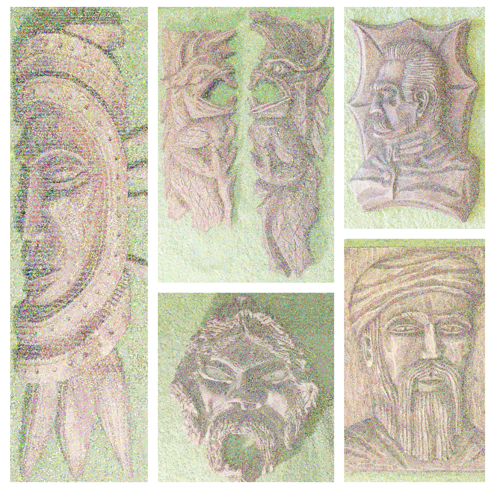
  41. Artiemjew, L. Collection of Artistic Works. Available online: http://el-art.com.pl (accessed on 5 May 2020).
  42. Artiemjew, L. The Image of Lech Artiemjew-Polish Mathematician, Sculptor, Painter and Musician. Available online: http://el-art.com.pl (accessed on 5 May 2020).
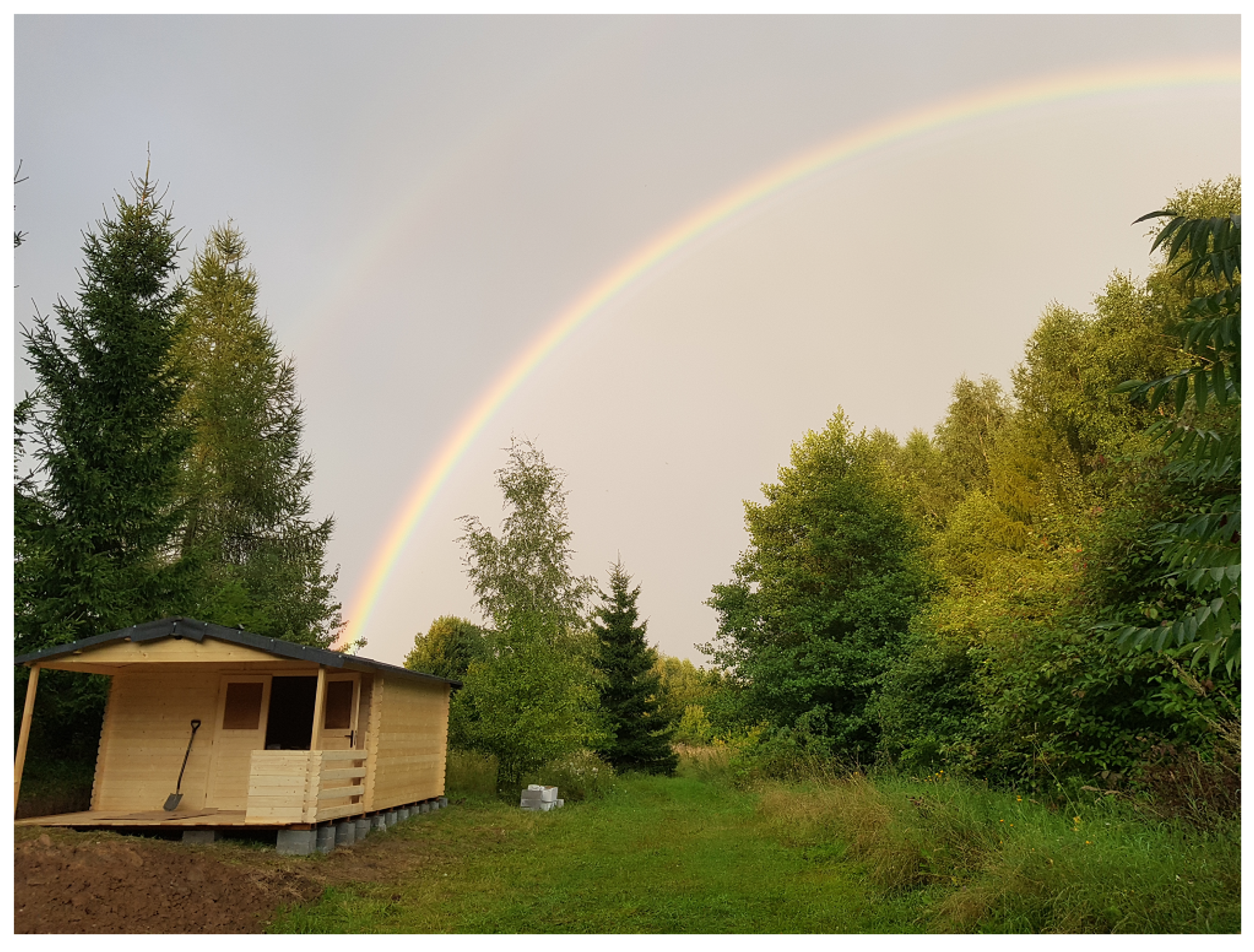
  43. Artiemjew, P. Macro Photography Collection. Available online: http://el-art.com.pl (accessed on 5 May 2020).
Figure 1. Changes in the red (R) color byte of R G B . We present the picture with the appropriate positions of Bytes changed to zero, from the top left corner to the rows, up to the bottom right we have, respectively changed 8 bits of Bytes, 7 and 8 bits of Bytes, , all bits of Bytes. You can see the limit of modification of the least significant bits of the image, in which we do not recognize the changes. The other colors have a zeroed eighth, least significant bit.
Computers 09 00038 g001
Figure 2. Changes in the green (G) color byte of R G B . We present the picture with the appropriate positions of Bytes changed to zero, from the top left corner to the rows, up to the bottom right we have, respectively changed 8 bits of Bytes, 7 and 8 bits of Bytes, , all bits of Bytes. You can see the limit of modification of the least significant bits of the image, in which we do not recognize the changes. The other colors have a zeroed eighth, least significant bit.
Computers 09 00038 g002
Figure 3. Changes in the blue (B) color byte of R G B . We present the picture with the appropriate positions of Bytes changed to zero, from the top left corner to the rows, up to the bottom right we have, respectively changed 8 bits of Bytes, 7 and 8 bits of Bytes, , all bits of Bytes. You can see the limit of modification of the least significant bits of the image, in which we do not recognize the changes. The other colors have a zeroed eighth, least significant bit.
Computers 09 00038 g003
Figure 4. Stegoanalisys-least significant bit (LSB) enhancement in a stego-carrier.
Computers 09 00038 g004
Figure 5. Stegoanalisys-LSB enhancement in a stego-carrier. You can clearly see the embedded message.
Computers 09 00038 g005
Figure 6. Stegoanalisys-LSB enhancement in a stego-carrier, randomly filled with information.
Computers 09 00038 g006
Figure 7. Communication process-steganographic system.
Computers 09 00038 g007
Figure 8. Our tests design.
Computers 09 00038 g008
Figure 9. Image for carrying information (cover picture).
Computers 09 00038 g009
Figure 10. Information to be hidden-Archimedes, bas-relief created by Reference [41].
Computers 09 00038 g010
Figure 11. Information to be hidden [42].
Computers 09 00038 g011
Figure 12. Information to be hidden-from the collection of macrophotography [43].
Computers 09 00038 g012
Figure 13. Stegoanalisys-LSB enhancement in a stego-carrier. The data is protected against detection by using the LSB Matching method (i.e., we also put the information in the second bit). In the example we used a 00 mask, and a 1 indistinguishability level. During embedding the information. In our experiment, we used pixels with a saturation range of [ 0 , 120 ] to distribute the uniform pixels.
Computers 09 00038 g013
Figure 14. Stegoanalisys-LSB enhancement in a stego-carrier. The data is protected against detection by using the LSB Matching method (i.e., we also put the information in the second bit). In the example we used a 00 mask, and a 1 indistinguishability level. During embedding the information, 24,319,784 empty slots were created, 1,273,791 least significant bits were changed. In our experiment, we used pixels with a saturation range of [ 0 , 120 ] to distribute the uniform pixels.
Computers 09 00038 g014
Figure 15. Stegoanalisys-LSB enhancement in a stego-carrier. The data is protected against detection by using the LSB Matching method (i.e., we also put the information in the second bit). In the example we used a 100 mask for R, 010 mask for G, 001 mask for B, and a 1 indistinguishability level. During embedding the information, 3,213,4402 empty slots were created, 1,295,702 least significant bits were changed. In our experiment, we used pixels with a saturation range of [ 0 , 200 ] to distribute the uniform pixels.
Computers 09 00038 g015
Figure 16. A picture with hidden information-there is Figure 10 hidden with use of mask 10.
Computers 09 00038 g016

