Model Structure Optimization for Fuel Cell Polarization Curves


Abstract
1. Introduction
2. Materials and Methods
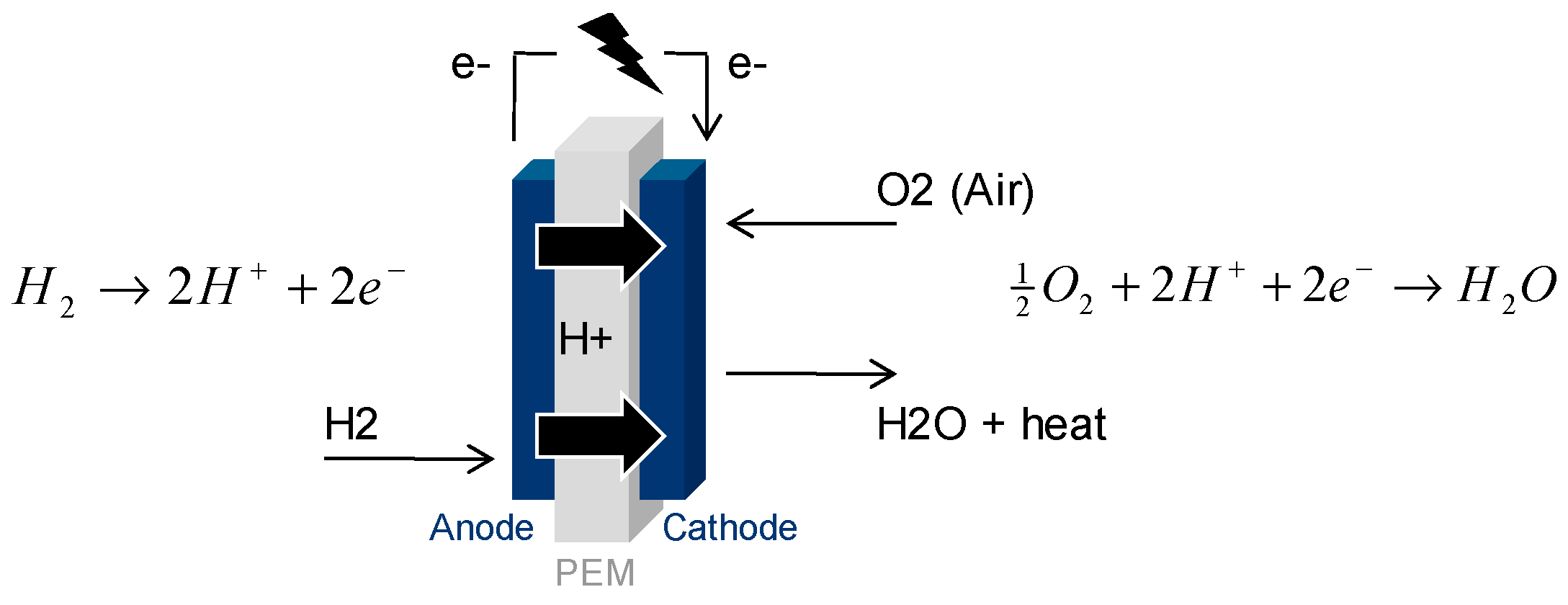
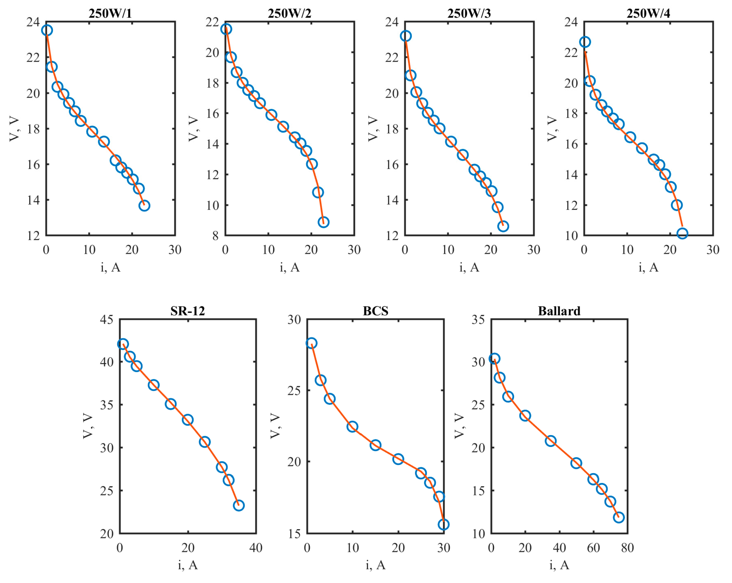
2.1. Fuel Cell Data
2.2. Reported Model Structures
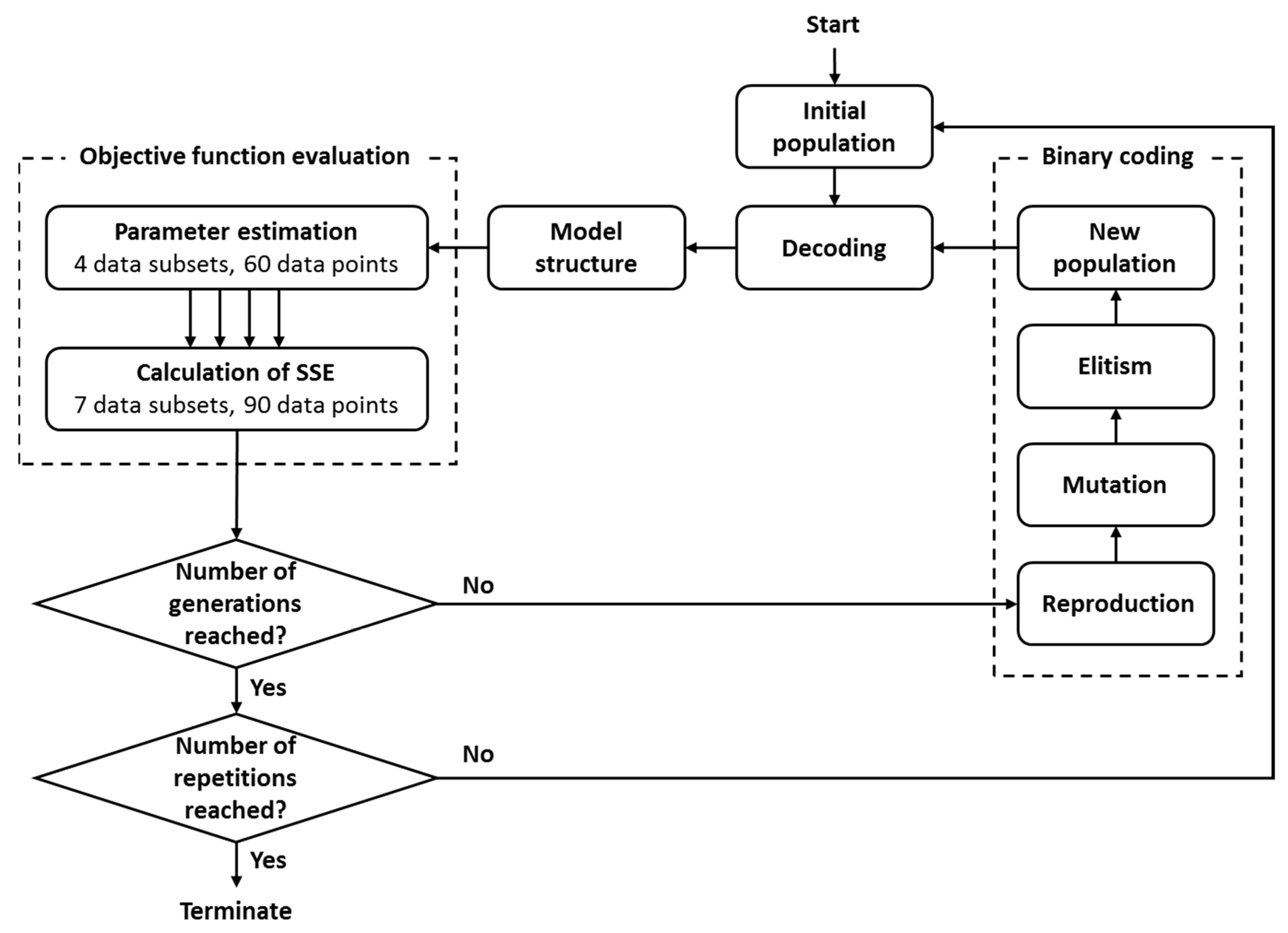
2.3. Algorithm for Model Structure Identification
2.3.1. Genetic Algorithms
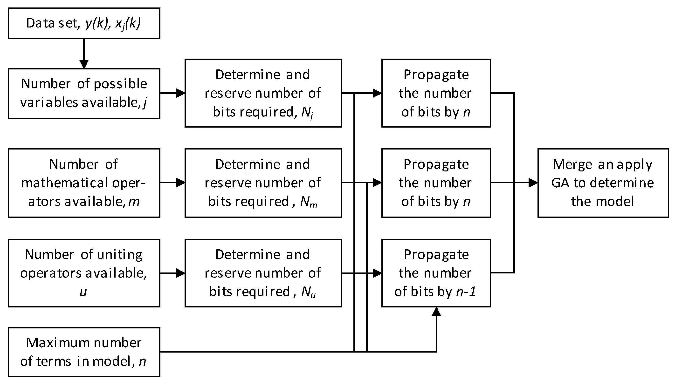
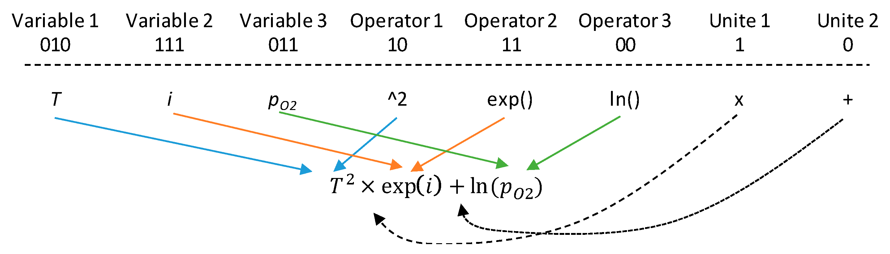
2.3.2. Chromosome Encoding and Decoding
2.3.3. Parameter Estimation
2.3.4. Objective Function and Model Performance
3. Results
3.1. Case 1
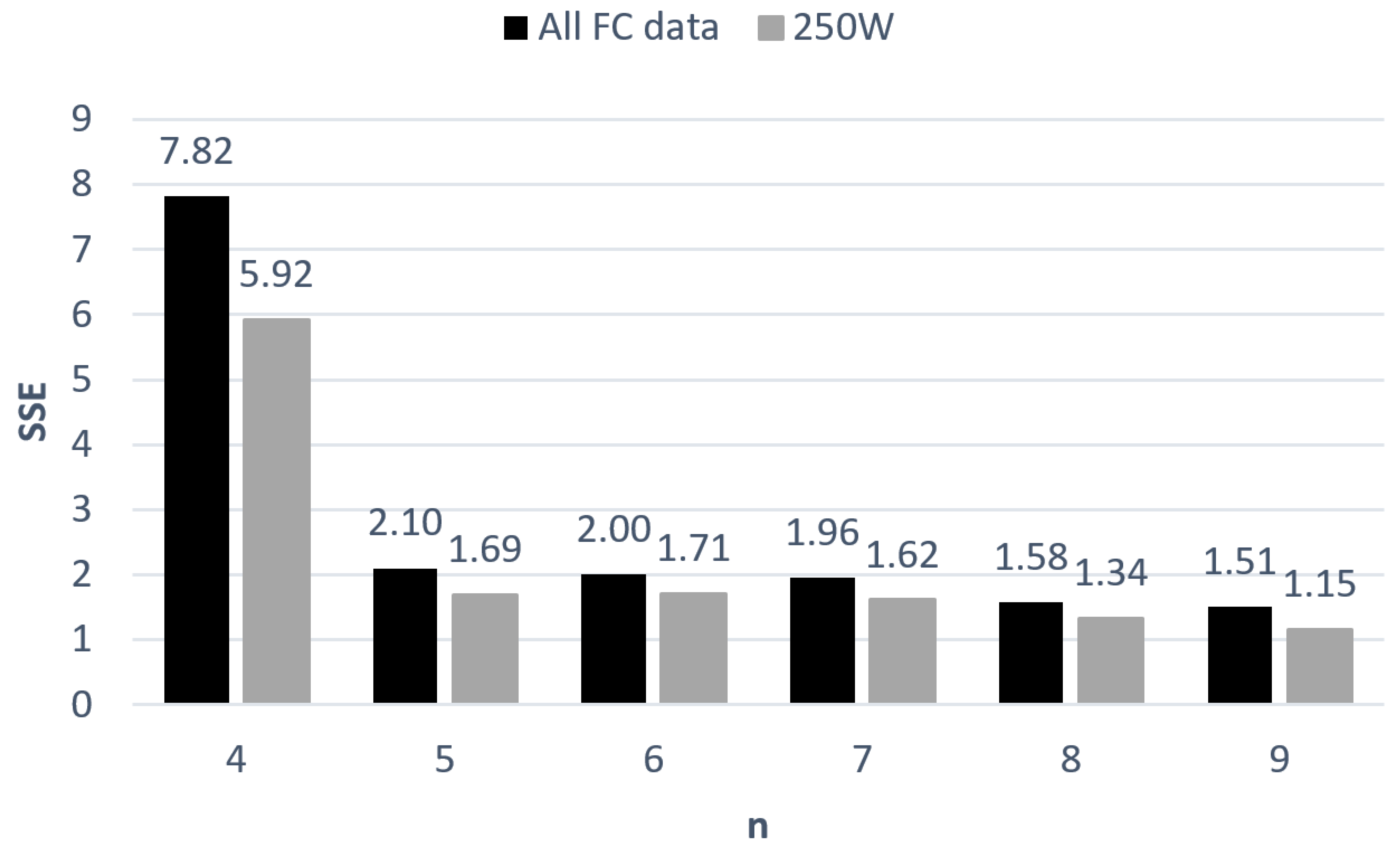
3.2. Case 2
3.3. Case 3
4. Discussion
5. Conclusions
Supplementary Materials
Author Contributions
Funding
Conflicts of Interest
Appendix A
References
- Sharaf, O.Z.; Orhan, M.F. An overview of fuel cell technology: Fundamentals and applications. Renew. Sustain. Energy Rev. 2014, 32, 810–853. [Google Scholar] [CrossRef]
- Lee, J.H.; Lalk, T.R.; Appleby, A.J. Modeling electrochemical performance in large scale proton exchange membrane fuel cell stacks. J. Power Sources 1998, 70, 258–268. [Google Scholar] [CrossRef]
- Mann, R.F.; Amphlett, J.C.; Hooper, M.A.I.; Jensen, H.M.; Peppley, B.A.; Roberge, P.R. Development and application of a generalised steady-state electrochemical model for a PEM fuel cell. J. Power Sources 2000, 86, 173–180. [Google Scholar] [CrossRef]
- Pisani, L.; Murgia, G.; Valentini, M.; D’Aguanno, B. A new semi-empirical approach to performance curves of polymer electrolyte fuel cells. J. Power Sources 2002, 108, 192–203. [Google Scholar] [CrossRef]
- Kulikovsky, A.A.; Wüster, T.; Egmen, A.; Stolten, D. Analytical and Numerical Analysis of PEM Fuel Cell Performance Curves. J. Electrochem. Soc. 2005, 152, A1290. [Google Scholar] [CrossRef]
- Amphlett, J.C. Performance Modeling of the Ballard Mark IV Solid Polymer Electrolyte Fuel Cell. J. Electrochem. Soc. 1995, 142. [Google Scholar] [CrossRef]
- Ohenoja, M.; Sorsa, A.; Leiviskä, K. Genetic Algorithms in Model Structure Identification for Fuel Cell Polarization Curve. In Proceedings of the 5th International Conference on Control, Decision and Information Technologies (CoDIT), Thessaloniki, Greece, 10–13 April 2018; pp. 539–544. [Google Scholar] [CrossRef]
- Jourdani, M.; Mounir, H.; Marjani, A. Three-Dimensional PEM Fuel Cells Modeling using COMSOL Multiphysics. Int. J. Multiphys. 2017, 11. [Google Scholar] [CrossRef]
- Mo, Z.-J.; Zhu, X.-J.; Wei, L.-Y.; Cao, G.-Y. Parameter optimization for a PEMFC model with a hybrid genetic algorithm. Int. J. Energy Res. 2006, 30, 585–597. [Google Scholar] [CrossRef]
- Ohenoja, M.; Leiviskä, K. Validation of genetic algorithm results in a fuel cell model. Int. J. Hydrogen Energy 2010, 35, 12618–12625. [Google Scholar] [CrossRef]
- Sorsa, A.; Koskenniemi, A.; Leiviskä, K. Differential evolution in parameter identification fuel cell as an example. In Proceedings of the 9th International Conference on Informatics in Control, Automation and Robotics (ICINCO 2012), Rome, Italy, 28–31 July 2012; Volume 1, pp. 40–49. [Google Scholar]
- Sun, Z.; Wang, N.; Bi, Y.; Srinivasan, D. Parameter identification of PEMFC model based on hybrid adaptive differential evolution algorithm. Energy 2015, 90, 1334–1341. [Google Scholar] [CrossRef]
- El-Fergany, A.A. Extracting optimal parameters of PEM fuel cells using Salp Swarm Optimizer. Renew. Energy 2018, 119, 641–648. [Google Scholar] [CrossRef]
- Ali, M.; El-Hameed, M.A.; Farahat, M.A. Effective parameters’ identification for polymer electrolyte membrane fuel cell models using grey wolf optimizer. Renew. Energy 2017, 111, 455–462. [Google Scholar] [CrossRef]
- Yang, S.; Chellali, R.; Lu, X.; Li, L.; Bo, C. Modeling and optimization for proton exchange membrane fuel cell stack using aging and challenging P systems based optimization algorithm. Energy 2016, 109, 569–577. [Google Scholar] [CrossRef]
- Chakraborty, U.K. Static and dynamic modeling of solid oxide fuel cell using genetic programming. Energy 2009, 34, 740–751. [Google Scholar] [CrossRef]
- Xue, X.D.; Cheng, K.W.E.; Sutanto, D. Unified mathematical modelling of steady-state and dynamic voltage–current characteristics for PEM fuel cells. Electrochim. Acta 2006, 52, 1135–1144. [Google Scholar] [CrossRef]
- Han, I.-S.; Chung, C.-B. Performance prediction and analysis of a PEM fuel cell operating on pure oxygen using data-driven models: A comparison of artificial neural network and support vector machine. Int. J. Hydrogen Energy 2016, 41, 10202–10211. [Google Scholar] [CrossRef]
- Srinivasan, S.; Ticianelli, E.A.; Derouin, C.R.; Redondo, A. Advances in solid polymer electrolyte fuel cell technology with low platinum loading electrodes. J. Power Sources 1988, 22, 359–375. [Google Scholar] [CrossRef]
- Kim, J. Modeling of Proton Exchange Membrane Fuel Cell Performance with an Empirical Equation. J. Electrochem. Soc. 1995, 142, 2670. [Google Scholar] [CrossRef]
- Squadrito, G.; Maggio, G.; Passalacqua, E.; Lufrano, F.; Patti, A. An empirical equation for polymer electrolyte fuel cell (PEFC) behaviour. J. Appl. Electrochem. 1999, 29, 1449–1455. [Google Scholar] [CrossRef]
- Correa, J.M.; Farret, F.A.; Canha, L.N.; Simoes, M.G. An electrochemical-based fuel-cell model suitable for electrical engineering automation approach. IEEE Trans. Ind. Electron. 2004, 51, 1103–1112. [Google Scholar] [CrossRef]
- Michalewicz, Z. Genetic Algorithms + Data Structures = Evolution Programs; Springer: Berlin/Heidelberg, Germany, 1996; ISBN 978-3-662-03315-9. [Google Scholar]
- Ohenoja, M.; Leiviska, K. Identification of electrochemical model parameters in PEM fuel cells. In Proceedings of the International Conference on Power Engineering, Energy and Electrical Drives, Lisbon, Portugal, 18–20 March 2009; pp. 363–368. [Google Scholar] [CrossRef]
- Chakraborty, U.K. Reversible and Irreversible Potentials and an Inaccuracy in Popular Models in the Fuel Cell Literature. Energies 2018, 11, 1851. [Google Scholar] [CrossRef]


| Ref. | np | i | Ptot | pO2 | ilim | CO2 | T | pH2 | RHa | RHc | Pa | Pc | A | Lm | ρm | E0 | |
|---|---|---|---|---|---|---|---|---|---|---|---|---|---|---|---|---|---|
| [19] | 2 | x | x | ||||||||||||||
| [20] | 3 | x | x | ||||||||||||||
| [2] | 5 | x | x | x | x | ||||||||||||
| [21] | 4 | x | x | x | |||||||||||||
| [6] | 10 | x | x | x | x | x | x | x | x | x | x | x | x | ||||
| [3] | 6 | x | x | x | x | x | x | x | x | x | x | x | x | x | x | ||
| [22] | 7 | x | x | x | x | x | x | x | x | x | x | x | x | x | x | x |
| Fuel Cell | SSE | |||
|---|---|---|---|---|
| Case 1 | Ohenoja et al. [24] | Ohenoja et al. [10] | Case 2 | |
| 250W/1 | 0.2384 | 0.2739 | ||
| 250W/2 | 0.2782 | 0.7142 | ||
| 250W/3 | 0.2059 | 0.3107 | ||
| 250W/4 | 0.8929 | 0.0476 | ||
| 250W/all | 1.6154 | 8.4854 | 1.3464 | |
| SR-12 | 0.0615 | 0.4475 | 0.5762 | |
| BCS | 0.2148 | 0.1040 | 0.1427 | |
| Ballard | 0.0640 | 0.0918 | 0.4825 | |
| Total SSE | 1.96 | 2.55 | ||
© 2018 by the authors. Licensee MDPI, Basel, Switzerland. This article is an open access article distributed under the terms and conditions of the Creative Commons Attribution (CC BY) license (http://creativecommons.org/licenses/by/4.0/).
Share and Cite
Ohenoja, M.; Sorsa, A.; Leiviskä, K. Model Structure Optimization for Fuel Cell Polarization Curves. Computers 2018, 7, 60. https://doi.org/10.3390/computers7040060
Ohenoja M, Sorsa A, Leiviskä K. Model Structure Optimization for Fuel Cell Polarization Curves. Computers. 2018; 7(4):60. https://doi.org/10.3390/computers7040060
Chicago/Turabian StyleOhenoja, Markku, Aki Sorsa, and Kauko Leiviskä. 2018. "Model Structure Optimization for Fuel Cell Polarization Curves" Computers 7, no. 4: 60. https://doi.org/10.3390/computers7040060
APA StyleOhenoja, M., Sorsa, A., & Leiviskä, K. (2018). Model Structure Optimization for Fuel Cell Polarization Curves. Computers, 7(4), 60. https://doi.org/10.3390/computers7040060