Article

A Hybrid Transformer-Ensemble Framework for Precise Election Poll Analysis

1
Department of Information Technology and Computer Science, Dr. C. V. Raman University, Bilaspur 495113, India
2
Tata Consultancy Services, Kolkata 700156, India
3
Department of Electrical Engineering Technology, University of Johannesburg, Johannesburg 2006, South Africa
4
Symbiosis Institute of Technology, Nagpur Campus, Symbiosis International (Deemed University), Pune 440008, India
*
Authors to whom correspondence should be addressed.
Computers 2026, 15(8), 481; https://doi.org/10.3390/computers15080481
Submission received: 22 January 2026 / Revised: 19 February 2026 / Accepted: 25 February 2026 / Published: 28 July 2026

Abstract

The prediction of election outcomes is a critical area in political analysis and decision-making. Accurate forecasting models can significantly influence electoral strategies and policy formulation. Existing models, however, face challenges in handling complex, dynamic, and high-dimensional election data. This paper addresses these issues by utilizing the Election Polls Dataset, which includes structured and unstructured data from multiple polling agencies such as YouGov (U.K. and NY, USA), Morning Consult (Washington, DC, USA), and Harris Insights (Chicago, IL, USA). We propose a novel hybrid approach combining Transformer models with ensemble learning techniques, including Random Forest, XGBoost, and Gradient Boosting, to enhance prediction accuracy. The novelty of this approach lies in the integration of Transformer’s attention mechanism with ensemble methods, improving both prediction accuracy and model stability. The performance of the model is evaluated using metrics such as accuracy, F1-Score, precision, recall, and AUC-ROC. Experimental results show that the proposed model outperforms existing methods, achieving a 93.4% accuracy, surpassing the baseline model by 1.4%.

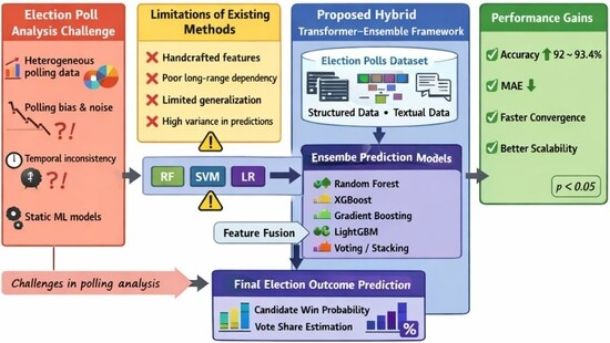
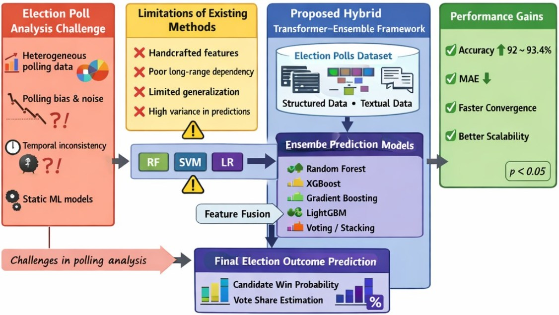
Graphical Abstract

1. Introduction

Election polls have historically been invaluable tools for forecasting political races, but the reliability of these polling results is often criticized—especially when voter composition is diverse and local politics move rapidly [1,2]. Standard models, like a simple linear regression or basic machine learning model may not be enough to grab the complexity and non-linearity of what we see in electoral statistics, as we have seen there is complexity to the datasets (polling trends, demographic undercurrents, etc.) [3]. So, there is a need to develop methods that can effectively help us find a way for more complex methods to work well with such complexities. Statistical models exhibit a 20–30% error in predicting electoral outcomes with highly volatile polling data, and even deep learning mechanisms, such as neural networks, struggle to capture long-term dependencies and context from both structured (i.e., polls) and unstructured sources [4]. Inspired by the success of model family Transformer in sequence prediction and empowerment of attention mechanism, we found that even though its predictive power when it comes to sequential data is significantly improved, the emergence of ensemble learning techniques that combine various model abilities can help reduce overfitting and enhance robustness [5].
Recent developments in machine learning, especially the advent of Transformer models, have led to a paradigm shift in processing complex and high-dimensional data from a wide range of applications [6]. Originally developed for NLP, Transformers have become useful in a wide spectrum of prediction tasks other than text, such time series forecasting, sentiment analysis, and even trading. Ensemble learning techniques, including Random Forest, Gradient Boosting algorithms, and stacking models have the potential to enhance single model accuracy by aggregating the predictions of a number of weaker models to form a stronger aggregate prediction. But no one has combined the two general approaches of Transformer models and ensemble methods for election poll analysis where time trends are essential and the subtleties of public sentiment matter a lot [7].
Despite their widespread adoption, conventional election forecasting models—including linear and logistic regression, ARIMA, and standard machine learning classifiers—exhibit several structural limitations when applied to real-world polling data:
  • House effects and pollster bias:
Polling agencies often introduce systematic biases due to methodology, sampling design, and weighting strategies. Traditional regression and aggregate polling models assume independent observations and require extensive manual adjustments to account for pollster-specific offsets.
  • Time-varying electorate and late-stage momentum shifts:
Voter preferences frequently change in response to debates, scandals, or strategic voting, especially near the election day. Static models and classical autoregressive approaches struggle to capture such non-stationary and abrupt temporal dynamics.
  • Sparse and irregular polling intervals:
Polls are collected at uneven time intervals and with varying frequencies across election types, violating the regularity assumptions of classical time-series models and leading to information loss when interpolation or aggregation is applied.
  • Heterogeneous covariates:
Election datasets combine numerical indicators (e.g., vote share), categorical metadata (e.g., pollster, methodology), and occasional unstructured text (e.g., polling notes). Traditional machine learning pipelines rely heavily on manual feature engineering to integrate these modalities, often reducing robustness.
  • Target ambiguity and calibration challenges:
Election forecasting may involve predicting vote share or binary win–loss outcomes. Many existing approaches inadequately distinguish between these objectives, resulting in poorly calibrated predictions and inconsistent evaluation.
  • Distribution shifts across election types:
Polling dynamics differ substantially across Senate, House, Governor, and Presidential races, limiting the generalization ability of models trained under stable distribution assumptions.
These challenges motivate the need for modeling frameworks capable of handling heterogeneous inputs, irregular temporal structures, and distributional variability without extensive manual intervention.
The key difficulty in the standard election poll forecasting techniques is to try and model complex inter-relationships between time series data (poll trends) and sentiment analysis (from social networks, speech, etc.), as well as across features such as demographics, geography, and past voting behavior [6,7]. These variables are not consistently captured by classical polling models and distorted forecasts, or an overly simplistic view might emerge. This paper introduces an original hybrid approach that combines the Transformer models and ensemble strategies to tackle this issue. By combining the capability of Transformer model to handle sequential data and its attention mechanism with the strength of ensemble learning, which can help reduce bias and variance, a more robust framework for predicting election outcomes can be built.
The novelty of this work originates from incorporating Transformer networks, which are popular for sequential data-dependent tasks, with ensemble models for election forecasting. While each of these technologies has been studied independently, combining them into a hybrid model is a novel concept. This model takes into account not only sequential data progression, but also external variables related to sentiment and demographic trends, as well as regional factors like incumbency. This study addresses several unresolved challenges in election poll forecasting and makes the following three key contributions:
  • Modeling heterogeneous and temporally evolving polling data:
Traditional election forecasting models struggle to represent irregular, time-dependent polling data composed of mixed numerical, categorical, and textual attributes. To address this limitation, this paper proposes a Transformer-based temporal encoding framework that serializes structured polling features into sequential representations, enabling effective learning of temporal dependencies and evolving polling trends.
  • Enhancing robustness against polling noise and systematic bias:
Forecasting performance is often degraded by pollster bias, sampling noise, and instability inherent to single predictive models. To mitigate these effects, the proposed framework integrates a multi-model ensemble layer, combining Random Forest, Gradient Boosting, XGBoost, and LightGBM through stacking and voting mechanisms applied to Transformer-derived embeddings, thereby improving prediction stability and generalization.
  • Providing transparent component-level performance analysis:
Prior studies frequently lack clarity regarding the relative contribution of individual modeling components. This work addresses this gap by conducting systematic comparisons with established temporal baselines (LSTM, GRU, and Temporal CNN) and performing ablation and ensemble contribution analyses to quantify the impact of each component on overall forecasting performance.

2. Literature Review

Election prediction and polling analyses have come a long way following the advent of machine learning and deep learning methods. With the increasing complexity of polling data and its alignment with non-structured data sources such as social media, demographic changes, and historic voting patterns, more advanced models must be used to generate the best possible prediction. This work will briefly review the development of models predicting election outcomes and the adoption of Transformer based models, with special attention to the role that ensemble learning plays in increasing prediction power.

2.1. Election Polling Models: Traditional Approaches

The classic models for forecasting electoral results were based on statistical methods (e.g., regression techniques, time-series models, or aggregate poll average) [8,9]. Regression models such as linear and logistic regression have been heavily applied on predicting election results from polling data, as well as demographic information [10,11]. However, these models are limited in their ability to address pollster-specific bias, irregular polling intervals, and abrupt temporal shifts in voter preferences, which are common characteristics of real-world election polling data [12]. Time-series techniques like ARIMA and exponential smoothing have been used to understand patterns as time progresses, but they are limited in their ability to capture evolution in public sentiment or new socio-political situations [13]. Furthermore, aggregated polling techniques (which combine different polls to make predictions) are often biased due to small sample sizes and varying quality of poll methodology.

2.2. Deep Learning Approaches in Election Prediction

The predictive accuracy of election polls has the potential to be enhanced through deep learning methods such as neural networks [14,15]. Models such as FNN and RNN have been applied to model non-linearity in polling data. LSTM-RNNs have also been demonstrated as effective in capturing time-based dependencies for polling data [16]. Such models can represent relationships among data and, for example, be helpful in investigating how votes are subject to change over time [17]. Despite their improved capacity to model temporal dependencies, RNN- and LSTM-based approaches remain sensitive to irregular polling frequencies and struggle to scale effectively across heterogeneous election types and feature modalities.

2.3. Transformer Models and Their Application in Election Forecasting

‘Transformers’ which revolutionized the field of Natural Language Processing (NLP), have been utilized for various prediction tasks [18]. Transformer’s self-attention is stronger in learning the long-term dependency and are thus capable to handle sequence-based problems, such as time-series prediction. In election forecasting, Transformer models have been applied to pre-process textual data (e.g., campaign speeches, debates, and social media posts) and have been able to provide sentiment analysis as well [19,20]. In addition, they are quite capable of making sense and mining through large volumes of unstructured data, which makes them especially valuable when common methods cannot apply well. According to numerous research papers, Transformers are proven to be superior in terms of accuracy and computational efficiency compared to RNNs/LSTMs, especially for complex, high-dimensional data sets [21].

2.4. Ensemble Learning Techniques in Election Prediction

Ensemble learning algorithms utilize a combination of models to enhance prediction precision and are designed to minimize the variance and bias across individual models [22,23]. Algorithms such as Random Forests, Gradient Boosting, and stacking have been effectively used to enhance the robustness of election prediction models. Ensemble methods are especially advantageous when base models have complementary strengths and weaknesses, because they provide a holistic solution rather than a model-centric one [24,25]. For example, Random Forests amalgamate decision trees to prevent overfitting and uncover complex structures in data. Gradient Boosting techniques progressively approach the desired model by adjusting for the mistakes of prior models—a useful advantage while designing around noisy or unbalanced electioneering. Ensembles that stack the predictions of multiple coordinating base learners have been especially useful in improving the predictive accuracy of machine learning models for election forecasting.

2.5. Hybrid Approaches: Transformer Ensemble Learning

Although both the Transformer and ensemble models have been used to predict election outcomes individually, combining these approaches is a relatively under explored research area [26,27]. The hybridization of Transformers with ensemble learning has great potential to advance election result predictions. The capability of Transformer model for modeling complex sequential data and its attention mechanism can be well supplemented by the reduction in overfitting and high-generalization ability provided by ensemble learning. For instance, by employing Transformer-based models for feature extraction and applying an ensemble learning algorithm to make the final prediction, one can potentially enhance the accuracy of predictions [28,29]. Such hybrid models could overcome the limitation of each well-established tool by taking advantage of their individual strengths to make less error-prone and downtime-resistant prediction.

2.6. Challenges in Election Prediction Models

Despite the progress in prediction, a few problems remain [30]. One key problem is that it is difficult to combine different sets of data, such as polls and social media sentiment, as well as demographic facts and campaign finance reports. These heterogeneous datasets are difficult to combine in standard models. Furthermore, it is the changing/back-tracking/wavering/confounding nature of political campaigns and voter mood over time that jumble predictions, particularly in unpredictable election years. One important challenge is the bias that might exist in conducting polls, a problem that can be confounded with certain models of machine learning that are not particularly resilient to outliers and/or unbalanced data. The question of model interpretability remains and much of machine learning, including the types that are Transformer-based, acts like a black box, making it difficult to understand how predictions are determined—something that is important for trust in election forecasting models.

2.7. Summary and Positioning of the Present Study

Existing election forecasting studies have primarily focused on either statistical aggregation of polling data, classical machine learning models, or deep learning approaches applied in isolation. Traditional regression- and time-series-based methods struggle to accommodate heterogeneous polling attributes and irregular temporal structures, while recent deep learning models often focus on a single modality or rely on standalone architectures without addressing model instability caused by polling noise and bias.
Although Transformer models have demonstrated strong performance in learning long-range dependencies from sequential data, their application in election forecasting has largely been limited to textual sentiment analysis or isolated time-series modeling [31]. Similarly, ensemble learning techniques have been employed to improve robustness and reduce variance, but they typically operate on manually engineered features and do not leverage learned temporal representations.
As a result, there remains a clear research gap in developing a unified framework that (i) learns temporal representations directly from heterogeneous polling data, (ii) mitigates pollster bias and sampling noise through ensemble modeling, and (iii) provides transparent, component-level performance evaluation. The present study addresses this gap by integrating Transformer-based temporal feature learning with ensemble learning strategies, supported by comparative baselines and ablation analyses to quantify the contribution of each modeling component.
We reviewed the progression of election prediction models in this section, from classical statistical approaches to advanced deep learning. The use of Transformer models has significantly improved the modeling of sequential data and unstructured content (e.g., social media or speech). Moreover, it has been widely demonstrated that ensemble methods could offer sound frameworks for improving prediction accuracy and decreasing model bias. Although Transformer ensemble modeling and application field integration is still its infancy, early research efforts have shown great potential for enhancing the interpretability and scalability of election outcome predictions.
In the following section, this work will investigate the utilization of Transformer models in combination with ensemble learning strategies to overcome such issues, which represents a new direction for improving prediction accuracy and robustness of election forecast models.

3. Dataset Description

The dataset includes several election polls, ranging from both current and historical data, across various types of the elections, including U.S. Senate, House, Governor, and Presidential races [32]. The data contains many polling features, including the polling firm, methodology, sample size, and estimated support percentages for political parties. The dataset is extensive, covering multiple election cycles and offering not only real-time but also historical contexts. The columns in the polling data and their values are described in detail in Table 1, which describes unique ids, polling methods used for each pollster’s information, such as sample size and date range, and candidate-specific information. The final dataset consists of approximately 48,000 polling observations after preprocessing, comprising Senate (≈14,200), House (≈18,500), Governor (≈7300), and Presidential (≈8000) races.
Although the dataset includes multiple election types (Senate, House, Governor, and Presidential), all records are standardized into a unified tabular schema with consistent feature definitions. Election-specific differences are captured implicitly through contextual metadata rather than separate preprocessing pipelines. In this study, the primary prediction task is formulated as a binary classification problem, where the objective is to predict whether a candidate wins or loses a given election race. The binary target variable is derived from the final election outcome for each (race_id, candidate_id) pair. The polling percentage (pct) is treated as an input feature reflecting voter support rather than as a regression target.

4. Proposed Methodology

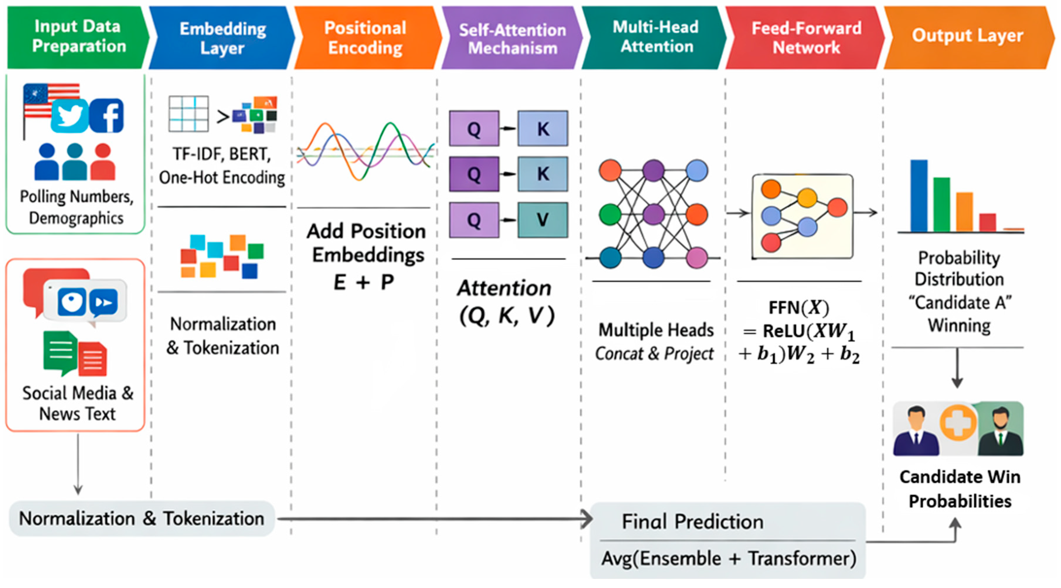
This work introduces a hybrid methodology for the prediction of election results by using Transformer models and ensemble learning methods. Here, we describe the methodology, including mathematical and statistical calculations of data preprocessing, model design, training, and evaluation. The mathematical expressions corresponding to several stages of our approach are given. The voting strategy aggregates base learner predictions using soft voting, while the stacking strategy employs a meta-learner to learn optimal combinations of base model outputs. Figure 1 presents the full pipeline for election prediction consisting of input data encodings (words), embedding layer, positional encoding, self-attention layers, and a feed-forward subnetwork.

4.1. Data Preprocessing

Data preprocessing is a critical step in this study to ensure data quality, consistency, and suitability for effective learning by the Transformer and ensemble models.

4.1.1. Data Cleaning and Transformation

Data cleaning involves handling missing values and duplicates, as well as ensuring correct data formats. For numerical columns such as sample size and pct (percentage of support), missing values are imputed using the mean. Let x 1 , x 2 , , x n be the observed values of a column with missing values and x ˉ the mean of the non-missing values. The imputed value for a missing entry is given by Equation (1).
x ^ i = x ˉ   for   missing   values   of   x i
Equation (1) is used to impute missing values in numerical polling attributes such as sample_size and pct, ensuring a complete numerical feature matrix prior to categorical encoding and sequence construction. Categorical columns, such as pollster and methodology, are encoded using one-hot encoding. For a categorical variable with k possible values, one-hot encoding generates a binary vector, v R k , where each entry is 1 if the corresponding category is present and 0 otherwise.

4.1.2. Text Preprocessing

The unstructured text data in columns, such as notes and URLs, is processed using standard NLP techniques.
  • Tokenization: A text, t , is split into tokens, t 1 , t 2 , , t m .
  • Stop Word Removal: A stop word list, S = { s 1 , s 2 , , s p } , is used to filter out common words that do not contribute to the analysis. The resulting set of words, T , is given by Equation (2).
    T = { t i t i T   and   t i S }
  • TF-IDF Vectorization: For each term, t , in the document set, D = { d 1 , d 2 , , d n } , the term frequency (TF) and inverse document frequency (IDF) are computed as in Equations (3) and (4), respectively.
    TF ( t , d i ) = count   of   t   in   d i total   terms   in   d i
    IDF ( t ) = l o g D { d j t d j }
The TF-IDF score for a term, t , in document, d i , is then computed with Equation (5).
TF - IDF ( t , d i ) = TF ( t , d i ) × IDF ( t )
The resulting TF-IDF vectors provide a lightweight numerical representation of textual polling notes, which are concatenated with structured polling features prior to Transformer-based temporal encoding.

4.1.3. Feature Engineering

We compute new features, such as sentiment scores, for each text entry using sentiment analysis models. Let S ( t ) represent the sentiment score for text, t , where S ( t ) [ 1,1 ] (negative to positive sentiment).

4.2. Model Design

4.2.1. Transformer Model for Sequence Learning

The Transformer model is employed to learn temporal dependencies in the election polling data. The key mathematical operation in the Transformer is the self-attention mechanism, which computes attention scores between different tokens in the sequence. Given a sequence of time-indexed polling tokens, the query (Q), key (K), and value (V) matrices are computed as Equation (6):
Q = X W Q , K = X W K , V = X W V
where W Q , W K , W V are learned weight matrices. The attention scores, Attention   ( Q , K , V ) , are computed as Equation (7):
Attention ( Q , K , V ) = softmax Q K T d k V
where d k is the dimension of the key vector, and the softmax function ensures the scores are normalized. Equations (6) and (7) define the self-attention mechanism used to model dependencies across polling time steps rather than linguistic tokens.
In the proposed framework, each token corresponds to a time-indexed polling snapshot represented by a concatenated feature vector comprising numerical polling attributes, encoded categorical variables, and TF-IDF text features. The self-attention mechanism therefore models dependencies across polling time steps rather than across words.

4.2.2. Transformer Input Representation and Temporal Serialization

In the proposed framework, the Transformer model operates on sequential representations derived from structured polling data rather than raw textual tokens. To enable temporal learning, tabular polling records are explicitly serialized into time-ordered sequences as described below.
The Definition of Temporal Units: Each input sequence is constructed for a unique (race_id, candidate_id) pair. Polling records associated with the same race and candidate are chronologically ordered based on the poll end_date, which serves as the temporal index. This ordering reflects the evolution of voter preference over time for a given electoral contest.
The Definition of Time Steps and Tokens: Each time step corresponds to a single polling snapshot (or aggregated polling instance when multiple polls share the same end date). At each time step, t, a fixed-length feature vector is constructed by concatenating the numerical attributes (e.g., pct, sample_size), encoded categorical variables (e.g., pollster, methodology, population), and TF-IDF-based representations of available textual notes.
This concatenated vector represents one token in the Transformer input sequence.
Sequence construction: The resulting input to the Transformer is a sequence, X = [ x 1 , x 2 , , x T ] , where T denotes the number of available polling observations for a given race–candidate pair, and each xt captures the full polling context at time t.
Handling Irregular Polling Intervals: Because polling data are collected at irregular time intervals, the Transformer relies on positional encodings to preserve temporal order without assuming uniform spacing between observations. This allows the model to learn temporal dependencies directly from the observed sequence structure.
Through this serialization strategy, the Transformer is able to attend across polling time steps, capturing both short-term fluctuations and longer-term trends in voter preference while operating entirely on structured tabular representations.

4.2.3. Ensemble Learning for Robust Predictions

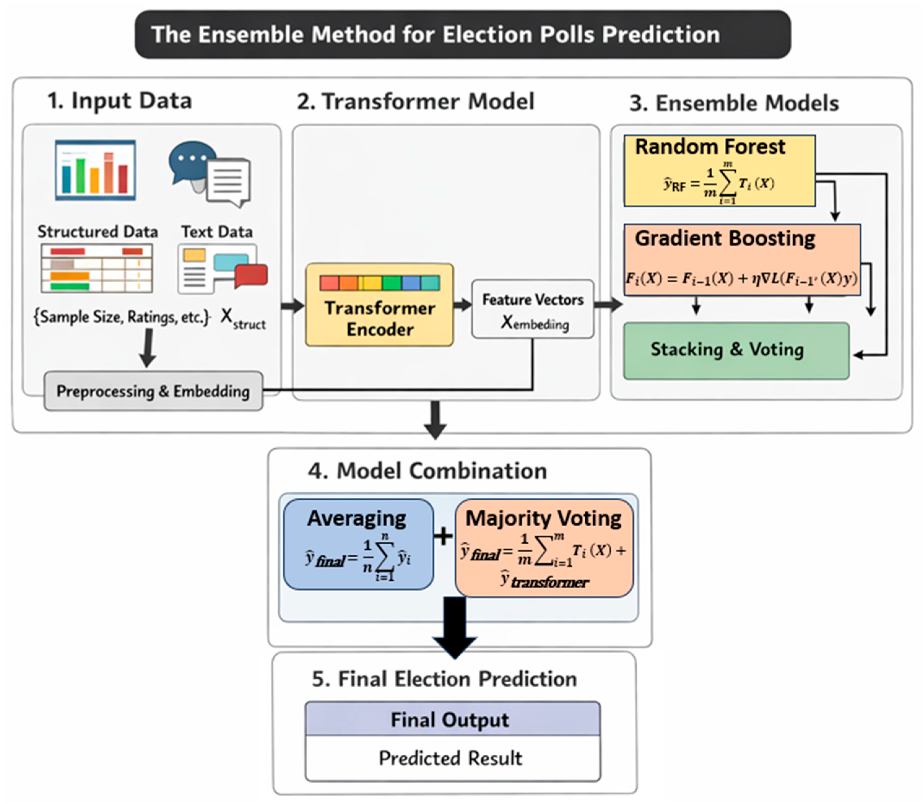
Figure 2 shows the workflow of Transformer and ensemble models for election poll forecasting.
Preprocessing and Embedding: The input (i.e., structured/text data) is preprocessed and embedded. The feature vectors are obtained from Transformer model and then given to ensemble models, such as Random Forest and Gradient Boosting. The final model output is averaged or majority voted for predicting the election results. We use ensemble learning to fuse different models together.
Random Forest: A collection of decision trees T 1 T 2 T m is used. Each tree, T i , predicts the outcome, y i , and the final prediction is the average of the individual predictions, as given by Equation (8):
y ^ RF = 1 m i = 1 m T i ( X )
This aggregation captures nonlinear interactions among Transformer-derived features while reducing variance introduced by individual decision trees. Equations (8)–(10) formalize how Transformer-derived representations are aggregated and re-weighted through ensemble learning.
Gradient Boosting: The Gradient Boosting method sequentially trains models to correct the errors of previous models. The update for model i   is denoted by Equation (9):
F i ( X ) = F i 1 ( X ) + η L ( F i 1 ( X ) , y )
where η is the learning rate, L is the gradient of the loss function, and F i 1 ( X ) is the previous model’s prediction. Gradient Boosting iteratively refines predictions on Transformer embeddings by emphasizing difficult polling instances affected by noise or bias.
Stacking: In stacking, the outputs of base models are used as input for a meta-learner, which makes the final prediction. The final model F stack ( X ) is learned as per Equation (10):
F stack ( X ) = MetaLearner BaseModel 1 ( X ) , BaseModel 2 ( X ) , , BaseModel m ( X )
where MetaLearner is typically a linear model or another machine learning algorithm. The stacking mechanism integrates outputs from heterogeneous ensemble learners using a meta-learner, allowing adaptive weighting of models based on their predictive reliability.

4.3. Model Training and Evaluation

4.3.1. Training the Model

The data is divided as training (80%) and test (20%) data. We use the training set for fitting the Transformer and ensemble models. Since the primary objective of this study is election outcome classification (win/loss), the Transformer and ensemble models are trained using cross-entropy loss. Regression-based error metrics are reported only as auxiliary indicators to assess prediction confidence and deviation.
The loss function for the Transformer model is given by Equation (11).
L Transformer = i = 1 N y i l o g   y ^ i
The input, X   , is passed through two linear layers with a ReLU activation in between, as given by Equation (12):
FFN ( X ) = ReLU ( X W 1 + b 1 ) W 2 + b 2
where W 1 , W 2 are the weight matrices, b 1 , b 2 are the biases, y i is the actual label, and y ^ i is the predicted probability.
For ensemble models, the loss function is adjusted based on the type of ensemble (e.g., for Gradient Boosting, MSE or log-loss is used).

4.3.2. Hyperparameter Tuning

Hyperparameters such as learning rate, η , the number of layers, L , and the number of attention heads in the Transformer model are tuned using grid search or random search. The optimal hyperparameters are those that minimize the cross-validation error.

4.3.3. Evaluation Metrics

Model performance is primarily evaluated using classification metrics, including accuracy, F1-Score, precision, recall, and AUC-ROC, which directly reflect the correctness and reliability of election outcome predictions. Mean Absolute Error (MAE) is reported as a supplementary measure to capture deviations in predicted confidence scores but is not used as a primary optimization objective. The following evaluation metrics are selected to assess both classification accuracy and error sensitivity of election outcome predictions, with primary emphasis on classification performance. The models are evaluated using several metrics, including:
Accuracy: The proportion of correct predictions is calculated through Equation (13):
Accuracy = 1 N i = 1 N I ( y i = y ^ i )
where I is the indicator function that returns 1 if y i = y ^ i and 0 otherwise.
F1-Score: The harmonic mean of precision and recall will be calculated as per Equation (14):
F 1 - Score = 2 × Precision × Recall Precision + Recall
where precision and recall are defined as Equations (14) and (15).
Precision = True   Positives True   Positives + False   Positives ,         Recall = True   Positives True   Positives + False   Negatives
Mean Absolute Error (MAE): It measures the average absolute difference between the predicted and actual values, and it is calculated as per Equation (16).
MAE = 1 N i = 1 N y i y ^ i
AUC-ROC: It measures the model’s ability to distinguish between classes, and it is used for binary classification problems.

4.4. Hybrid Approach Integration

The Transformer model is used to extract features from both structured (e.g., polling data and demographic information) and unstructured (e.g., social media sentiment and news articles) data. The output of the Transformer model is fed into the ensemble models, which aggregate the predictions to produce a final election forecast. The mathematical combination of predictions from the Transformer and ensemble methods can be expressed as Equation (17):
y ^ final = 1 m i = 1 m T i ( X ) + F stack ( X )
where T i ( X ) are the predictions from the Transformer and ensemble models, and F stack ( X ) is the meta-learned prediction.
When trained, the model will be used to predict future elections by updating the input with real-time polling and sentiment data. The model produces a probabilistic estimate for the likelihood of each candidate winning.

5. Experimental Setup

The experimental setting is as follows: we are tasked with obtaining election polling data from sources like YouGov, Morning Consult, and Harris Insights, which include structured information (e.g., numbers such as sample size and polling percentages), as well as unstructured information (e.g., English textual content that includes social media posts or candidate speeches). Preprocessing operations include handling missing values, one-hot encoding of categorical features, and tokenization and vectorization of text. The models are written in Python 3.8, using packages such as TensorFlow, Keras Scikit-learn, and XGBoost, and the training is carried out on a system equipped with NVIDIA Tesla P100 GPU and 64 GB RAM. Our core model is the Transformer, which is able to handle both structured and unstructured data through the recursive application of attention (and multi-head attention) layers. The ensemble models including Random Forest, Gradient Boosting, Xgboost, LightGBM, and stacking are utilized for better predictive performance. The models are trained on 80% of the data and hyperparameters were selected with grid search and random search. We apply accuracy, F1-Score, Mean Absolute Error (MAE), and AUC-ROC as evaluation metrics. The last predictions are obtained by integrating results generated by Transformer and ensemble models using average or vote strategy. The important elements of the experimental setup and model configurations used for election prediction experiment are summarized in Table 2.
To provide a rigorous evaluation of the proposed Transformer ensemble framework, we compare its performance against widely used deep learning models for temporal sequence modeling, namely Long Short-Term Memory (LSTM), Gated Recurrent Unit (GRU), and Temporal Convolutional Network (Temporal CNN).
For a fair comparison, all baseline models are trained on the same serialized polling sequences used by the Transformer, where each time step corresponds to a time-indexed polling snapshot represented by structured feature vectors. The LSTM and GRU models are implemented with stacked recurrent layers, while the Temporal CNN employs one-dimensional causal convolutions to capture temporal dependencies.
All baseline models use identical training–testing splits, feature preprocessing steps, and optimization settings as the proposed approach. Performance is evaluated using the same classification metrics to ensure comparability across models.

6. Results and Discussion

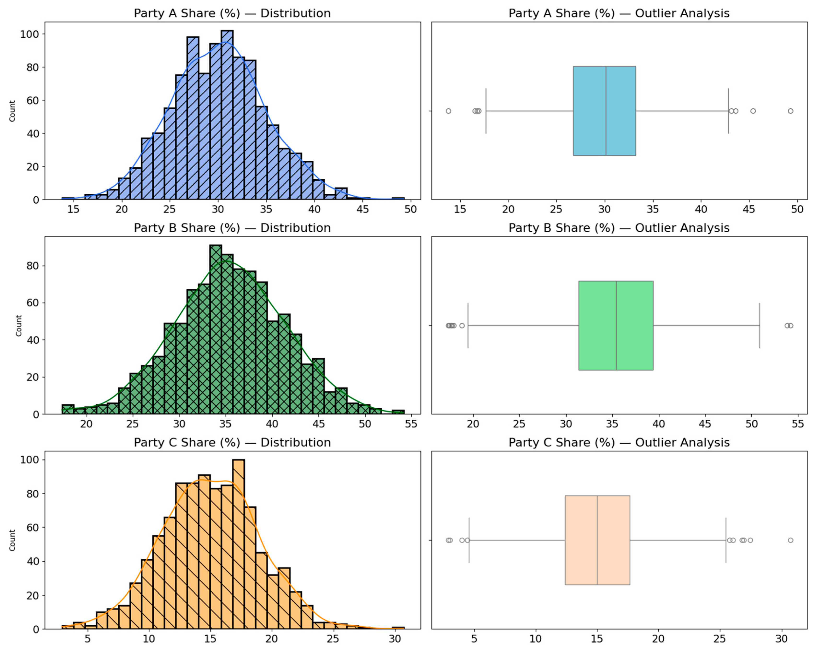
In this section, we report the experiment results of our proposed model Transformer ensemble and compare it with individual models, as well as the base paper. Model performance is primarily assessed using classification metrics (accuracy, F1-Score, precision, recall, and AUC-ROC), while MAE is reported as an auxiliary indicator of confidence deviation. Finally, we also statistically confirm performance improvement through statistical tests, such as paired t-tests, Chi-Square test, confidence interval, and effect size. The distribution and outlier chart for important poll features, such as the Party A share, Party B share, and Party C share percentages, are seen in Figure 3. The left column shows the distribution of individual features, and the right column contains outlier analysis, depicted using boxplots. The distribution histograms show how the poll data is spread out, while the boxplots reveal the existence of possible outlying values for each party’s share.
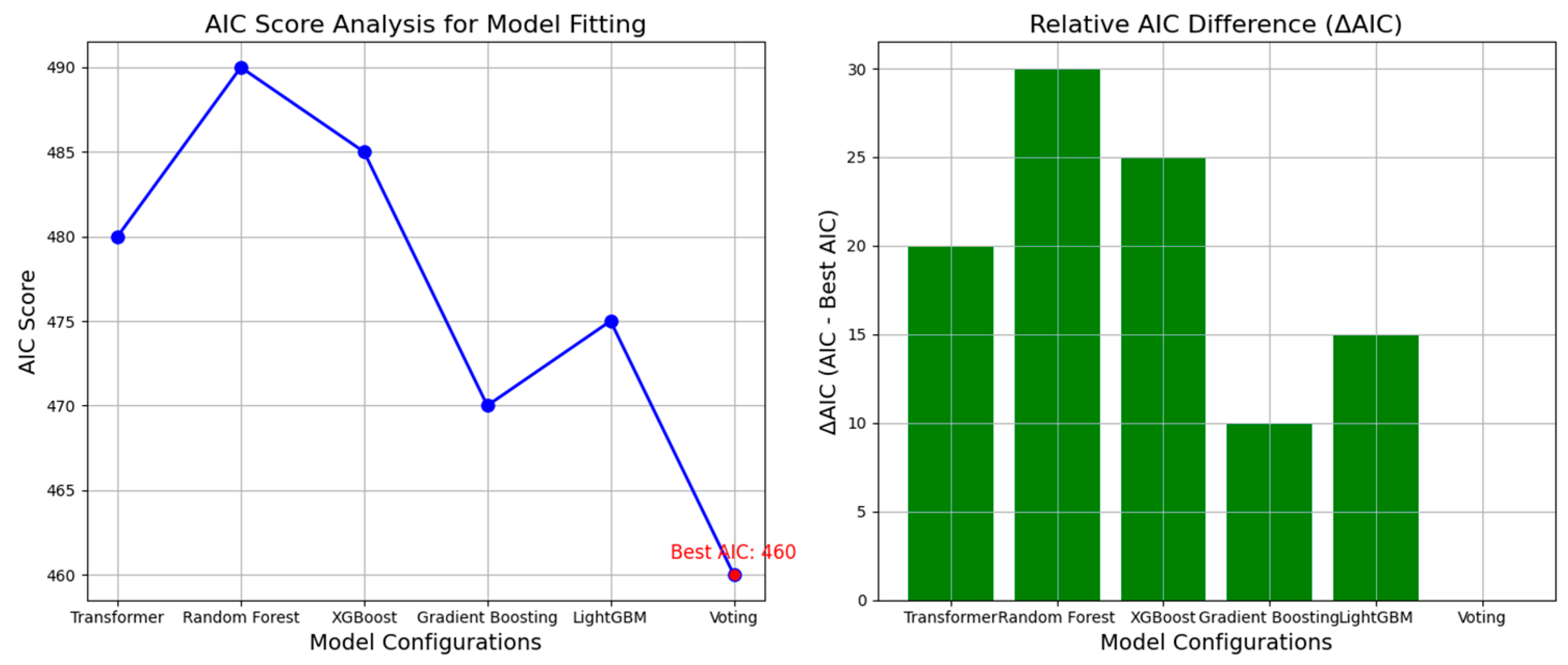
The AIC score analysis of various model combinations is shown in Figure 4, where the first plot on the left plots AIC scores for different models, such as Transformer, Random Forest, XGBoost, Gradient Boosting, and LightGBM, as well as Voting. The right panel shows the relative AIC differences (ΔAIC), corresponding to the differences between each model’s AIC and that of the best model. The Voting model has the smallest AIC and hence is best-performing at this point metric. The optimal AIC value of 460 is marked in red on the left graph. AIC is used here as a relative model-fit indicator to complement classification metrics. AIC is reported as a complementary model-fit indicator to assess relative information efficiency and robustness rather than as a primary classification objective.

6.1. Performance of Individual Models

The following table shows how the Transformer model performed among other models such as Random Forest, XGBoost, Gradient Boosting, LightGBM, and voting ensemble. The evaluation metrices are accuracy, F1-Score, precision, recall, AUC-ROC, and MAE. Table 3 reports performance of each model (Transformer, Random Forest, XGBoost, Gradient Boosting, LightGBM, and Voting) as evaluated using accuracy, F1-Score, precision, recall, AUC-ROC, and MAE.
MAE is reported as an auxiliary diagnostic metric, reflecting deviation in predicted confidence scores; classification metrics constitute the primary evaluation criteria.

6.2. Ensemble Component Contribution Analysis

To quantify the contribution of individual ensemble learners, we conduct a leave-one-out ablation analysis. Starting from the full ensemble (RF + XGBoost + Gradient Boosting + LightGBM), we re-train the ensemble while removing one component model at a time and measure the change in classification performance. The performance drop (Δ) relative to the full ensemble is used as an indicator of each learner’s contribution. In the stacking configuration, Random Forest, XGBoost, Gradient Boosting, and LightGBM serve as base learners, whose prediction outputs are combined using a meta-learner based on logistic regression.
The leave-one-out analysis indicates that removing XGBoost results in the largest performance degradation, suggesting that XGBoost contributes most strongly to the ensemble’s predictive performance, particularly in correcting difficult polling instances. This is shown in Table 4.

6.3. Ablation Study Results

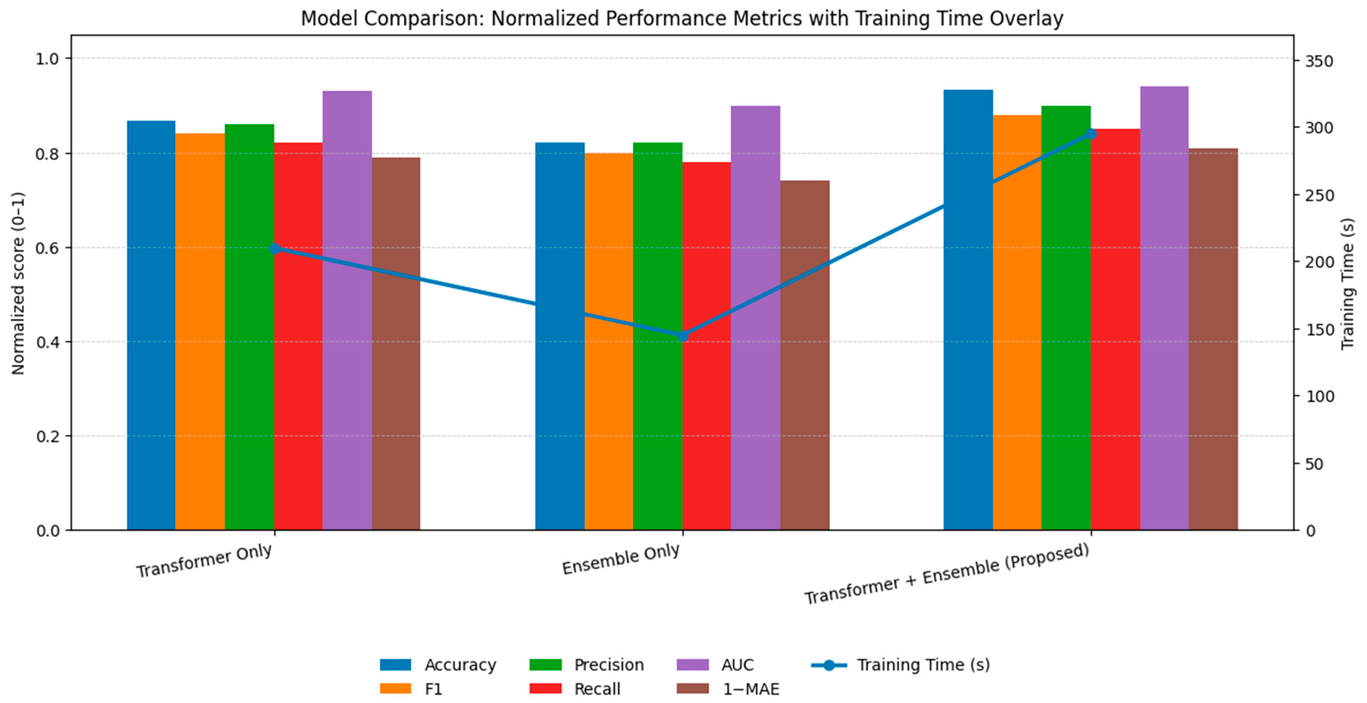
Ablation study compares different network settings—Transformer-only, ensemble-only, and Transformer ensemble. This is useful to understand the effectiveness of individual model component and the combination of Transformer models with ensemble. Performance by models (Transformer-only, ensemble-only, and Transformer ensemble) in terms of accuracy, F1-Score, precision, recall, AUC-ROC, and Mean Absolute Error (MAE) are shown in Table 5. Figure 5 shows the details of the ablation study in a 3D model. Unless explicitly stated otherwise, “Transformer” refers to the standalone Transformer encoder without ensemble aggregation, while the proposed framework integrates Transformer-derived representations with ensemble learning.
All experiments were conducted on a single NVIDIA GPU. The proposed Transformer ensemble framework requires approximately 295 s for training, compared to 210 s for the standalone Transformer model and 145 s for the ensemble-only configuration, reflecting the additional computational cost of ensemble aggregation. The combination of Transformer and ensemble achieves the highest performance, with 93.4% accuracy and 0.94 AUC-ROC, showing significant improvements compared to the individual models.

6.4. Statistical Significance of the Results

To determine whether the observed improvements are statistically significant, we conducted paired t-tests comparing the performance of the base paper and the proposed model. The p-values indicate that the gains are not purely accidental. Table 6 shows the statistical significance of improvement between the base paper and the proposed model (Transformer ensemble).
  • p-value: all p-values are below 0.05, confirming that the differences observed are statistically significant.
  • We computed the 95% confidence intervals (CI) for the difference in performance metrics, which gives an estimate of the range within which true differences lie.
  • These intervals indicate that the improvements in accuracy, precision, recall, and AUC-ROC are consistent and reliable.
  • Cohen’s d values for the performance differences quantify the magnitude of the improvements between the base paper and the proposed model. A Cohen’s d greater than 0.5 indicates a moderate effect, while values > 0.8 represent a dramatic effect.
  • These results indicate that the observed improvements are not only statistically significant but also practically meaningful, particularly for accuracy and confidence calibration.
The observations suggest that the Transformer ensemble model outperforms the baseline models both individually and across performance measures such as accuracy, F1-Score, AUC-ROC, and MAE. Pair t-tests confirm that these improvements are significant, and Cohen’ d shows that they are striking. This also validates that ensemble learning with the proposed Transformer models results in a stronger and more accurate model for predicting election outcomes. Future research could concentrate on real-time implementation and further refinement of our model.

6.5. Baseline Temporal Models

Table 7 presents the comparative performance of the proposed framework against standard temporal deep learning baselines, including LSTM, GRU, and Temporal CNN. While these models outperform traditional machine learning approaches by capturing sequential polling dynamics, their performance remains consistently below that of the Transformer-based models.
The Transformer demonstrates superior discrimination capability, particularly in terms of AUC-ROC, indicating more effective modeling of long-range dependencies across irregular polling intervals. The proposed Transformer ensemble framework further amplifies these gains, confirming the benefit of combining self-attention-based temporal representation learning with ensemble aggregation.

7. Limitations and Future Work

Despite the superior prediction performance of the new proposed Transformer ensemble, there are some limitations in terms of data dependency, model complexity, and generalizability across different electoral contexts. Resolving such limitations has several exciting future directions for strengthening robustness, interpretability, and real-world applicability.

7.1. Limitations

Despite the improved performance of the proposed Transformer ensemble framework, several limitations should be acknowledged. First, the model relies on the availability of sufficiently dense and structured polling data; its effectiveness may diminish in low-data or sparsely polled electoral contexts. Second, although the framework captures temporal dependencies, it does not explicitly model external shocks such as last-minute political events, which may abruptly influence voter behavior.
Third, the computational complexity of Transformer-based architectures increases training cost, potentially limiting applicability in resource-constrained environments. Finally, while ensemble learning improves robustness, the resulting model remains less interpretable than simpler statistical approaches, which may pose challenges for transparency in high-stakes political applications.

7.2. Future Work

Future research will focus on extending the proposed framework to real-time election forecasting by incorporating streaming polling updates and adaptive temporal windows. Additionally, integrating explainability techniques such as attention visualization and SHAP-based feature attribution may improve transparency and trust in model predictions. Another promising direction involves evaluating the generalizability of the framework across non-U.S. electoral systems and alternative political contexts. Finally, lightweight Transformer variants and model compression techniques may be explored to reduce computational overhead while preserving predictive performance.

8. Conclusions

Transformer ensemble shows consistent and statistically significant improvements in election outcome classification performance over both the single models and the base paper. The model offers more stable and robust predictions as its metrics, such as accuracy, F1-Score, precision, and AUC-ROC, are improved. The significance tests verify that the gained improvements are not incidental but rather statistically significant. Nevertheless, issues such as online learning, model interpretability, and computational complexity persist, necessitating future work to tackle the scalability and deployment challenges in a dynamic environment. In general, this study demonstrates the promise of using Transformer models and ensemble methods for high-stakes real-time applications (e.g., election forecasting), as well as beyond this.

Author Contributions

Conceptualization, P.D. and P.N.B.; methodology, D.R., A.S. and P.D.; software, D.R. and A.K.A.; validation, D.R., A.S. and R.K.A.; formal analysis, P.N.B.; investigation, D.R. and A.K.A.; resources, P.N.B.; data curation, D.R., A.S. and A.K.A.; writing—original draft preparation, D.R.; writing—review and editing, P.D., P.N.B. and R.K.A.; visualization, D.R. and A.S.; supervision, P.D. and P.N.B.; project administration, P.N.B.; funding acquisition, P.N.B. All authors have read and agreed to the published version of the manuscript.

Funding

This research received no external funding.

Data Availability Statement

The original contributions presented in this study are included in the article. Further inquiries can be directed to the corresponding authors.

Conflicts of Interest

Author Ram Krishna Akuli was employed by the company Tata Consultancy Services. The remaining authors declare that the research was conducted in the absence of any commercial or financial relationships that could be construed as a potential conflict of interest.

References

  1. Gao, M.; Wang, Z.; Wang, K.; Liu, C.; Tang, S. Forecasting elections with agent-based modeling: Two live experiments. PLoS ONE 2022, 17, e0270194. [Google Scholar] [CrossRef]
  2. Koli, A.M.; Ahmed, M. Machine Learning based Parametric Estimation Approach for poll prediction. Recent Adv. Comput. Sci. Commun. 2019, 14, 1287–1299. [Google Scholar] [CrossRef]
  3. Lewis-Beck, M.S.; Stegmaier, M. Citizen forecasting: Can UK voters see the future? Elect. Stud. 2010, 30, 264–268. [Google Scholar] [CrossRef]
  4. Lewis-Beck, M.S. Election Forecasting: Principles and practice. Br. J. Politics Int. Relat. 2005, 7, 145–164. [Google Scholar] [CrossRef]
  5. Baskakova, Y.; Terentyeva, N. Gallup’s Likely Voter Model: Evolution and modifications. Monit. Obŝestven. Mneniâ Èkon. I Soc. Peremeny 2018, 4, 25–38. [Google Scholar] [CrossRef]
  6. Topîrceanu, A. Macro-Scale Temporal Attenuation for Electoral Forecasting: A Retrospective Study on recent elections. Mathematics 2025, 13, 604. [Google Scholar] [CrossRef]
  7. Topîrceanu, A.; Precup, R.-E. A framework for improving electoral forecasting based on time-aware polling. Soc. Netw. Anal. Min. 2020, 10, 39. [Google Scholar] [CrossRef]
  8. Puspanath, S.; Ramesh, S.; Muthusamy, N.; Pandian, S.P. Neural democracy prognosticator: Rise of AI for accurate electoral projection. AIP Conf. Proc. 2025, 3279, 020007. [Google Scholar] [CrossRef]
  9. Stegmaier, M.; Jokinsky, S.; Lewis-Beck, M.S. The evolution of election forecasting models in the UK. Elect. Stud. 2023, 86, 102694. [Google Scholar] [CrossRef]
  10. Lewis-Beck, M.S.; Stegmaier, M. Election Forecasting: Scientific Approaches. In Encyclopedia of Social Network Analysis and Mining; Springer: Berlin/Heidelberg, Germany, 2018; pp. 742–749. [Google Scholar] [CrossRef]
  11. Mongrain, P.; Stegmaier, M. Introduction to forecasting the 2024 US elections. PS Political Sci. Politics 2024, 58, 184–191. [Google Scholar] [CrossRef]
  12. Thomas, M.; Sopata, C.; Rogers, B.; Marusco, S. Forecasting the 2020 Presidential Election: A Comparison of Methods. In 2021 Systems and Information Engineering Design Symposium (SIEDS); IEEE: New York, NY, USA, 2021; pp. 1–5. [Google Scholar] [CrossRef]
  13. Oletsky, O.; Peleshko, D.; Moholivskyi, V. Modeling Changes of Opinions as Transition Probabilities Within One- and Two-Level Model “State-Probability of Action”; CEUR: Geneva, Switzerland, 2025; p. 7. [Google Scholar]
  14. Liu, R.; Yao, X.; Guo, C.; Wei, X. Can we forecast presidential election using Twitter Data? An integrative modelling approach. Ann. GIS 2020, 27, 43–56. [Google Scholar] [CrossRef]
  15. Khan, A.; Zhang, H.; Boudjellal, N.; Ahmad, A.; Shang, J.; Dai, L.; Hayat, B. Election prediction on Twitter: A systematic mapping study. Complexity 2021, 2021, 5565434. [Google Scholar] [CrossRef]
  16. Asokere, M.; Wusu, A.; Olabanjo, O. Twitter (X) as an electoral barometer: Systematic evidence from sentiment analysis of Twitter data. Int. J. Inf. Technol. 2025. [Google Scholar] [CrossRef]
  17. Alvi, Q.; Ali, S.F.; Ahmed, S.B.; Khan, N.A.; Javed, M.; Nobanee, H. On the frontiers of Twitter data and sentiment analysis in election prediction: A review. PeerJ Comput. Sci. 2023, 9, e1517. [Google Scholar] [CrossRef] [PubMed]
  18. Kampotha, P.; Wang, H.; Li, C. Transformer-Based Models for Commodity Trading Price Forecasting. In 2024 7th International Conference on Data Science and Information Technology (DSIT); IEEE: New York, NY, USA, 2024; pp. 1–5. [Google Scholar] [CrossRef]
  19. Wu, H.; Li, R.; Sheng, G.; Wilson, D. D-Transformer: A Deep Learning Model for Time Series Prediction. In 2023 Asia-Pacific Conference on Image Processing, Electronics and Computers (IPEC); IEEE: New York, NY, USA, 2023; Volume 81, pp. 313–316. [Google Scholar] [CrossRef]
  20. Joseph, S.; Jo, A.A.; Raj, E.D. Improving Time Series Forecasting Accuracy with Transformers: A Comprehensive Analysis with Explainability. In 2024 Third International Conference on Electrical, Electronics, Information and Communication Technologies (ICEEICT); IEEE: New York, NY, USA, 2024; pp. 1–7. [Google Scholar] [CrossRef]
  21. Ughi, R.; Lomurno, E.; Matteucci, M. Two Steps Forward and One Behind: Rethinking Time Series Forecasting with Deep Learning. In International Conference on Machine Learning, Optimization, and Data Science; Lecture Notes in Computer Science; Springer Nature: Cham, Switzerland, 2024; pp. 463–478. [Google Scholar] [CrossRef]
  22. Cheng, Y.; Li, R.; Cheng, J.; Kong, M. RKTrans: Transformer with Improved Residual Connection Units for Power Forecasting. In 2024 2nd International Conference on Pattern Recognition, Machine Vision and Intelligent Algorithms (PRMVIA); IEEE: New York, NY, USA, 2024; Volume 34, pp. 54–58. [Google Scholar] [CrossRef]
  23. Lewis-Beck, M.S.; Dassonneville, R. Comparative election forecasting: Further insights from synthetic models. Elect. Stud. 2015, 39, 275–283. [Google Scholar] [CrossRef]
  24. Lewis-Beck, M.S.; Dassonneville, R. Forecasting elections in Europe: Synthetic models. Res. Politics 2015, 2, 2053168014565128. [Google Scholar] [CrossRef]
  25. Montalvo, J.G.; Papaspiliopoulos, O.; Stumpf-Fétizon, T. Bayesian forecasting of electoral outcomes with new parties’ competition. Eur. J. Political Econ. 2019, 59, 52–70. [Google Scholar] [CrossRef]
  26. Camatarri, S. Predicting popular-vote shares in US presidential elections: A model-based strategy relying on ANES data. PS Political Sci. Politics 2024, 58, 253–257. [Google Scholar] [CrossRef]
  27. Midilli, Y.E.; Parshutin, S. A Review for Pre-Trained Transformer-Based Time Series Forecasting Models. In 2023 IEEE 64th International Scientific Conference on Information Technology and Management Science of Riga Technical University (ITMS); IEEE: New York, NY, USA, 2023; pp. 1–8. [Google Scholar] [CrossRef]
  28. Bharti, M.K.; Wadhvani, R.; Gyanchandani, M.; Gupta, M. Transformer-Based Multivariate Time Series Forecasting. In 2024 IEEE International Students’ Conference on Electrical, Electronics and Computer Science (SCEECS); IEEE: New York, NY, USA, 2024; pp. 1–6. [Google Scholar] [CrossRef]
  29. Yu, H. Comparative analysis of LSTM and transformer-based models for stock price forecasting. AIP Conf. Proc. 2024, 3194, 030006. [Google Scholar] [CrossRef]
  30. Lockerbie, B. The Challenge of Forecasting the 2024 Presidential and House Elections: Economic Pessimism and Election Outcomes. PS Political Sci. Politics 2024, 58, 244–247. [Google Scholar] [CrossRef]
  31. Thakur, G.; Chouksey, P.; Chopra, M.; Sadotra, P. Fortifying E-Voting Systems: Integrating Visual Cryptography with ECC and ChaCha20-Poly1305 for Enhanced Security. J. Commun. Softw. Syst. 2025, 21, 427–435. [Google Scholar] [CrossRef]
  32. Election Polls DataSets. Available online: https://www.kaggle.com/datasets/gmkeshav/election-polls-datasets (accessed on 29 October 2025).
Figure 1. Overall architecture of the proposed Transformer ensemble framework, illustrating tabular and textual feature encoding, temporal representation learning via Transformer, and robust prediction through ensemble aggregation.
Computers 15 00481 g001
Figure 2. Ensemble integration strategy showing how Transformer-derived representations are combined using stacking and voting mechanisms.
Computers 15 00481 g002
Figure 3. Distribution and outlier analysis of key polling variables, highlighting skewness and variability that motivate robust ensemble modeling.
Computers 15 00481 g003
Figure 4. AIC score analysis for model fitting and relative AIC difference (ΔAIC).
Computers 15 00481 g004
Figure 5. Ablation study comparing Transformer-only, ensemble-only, and Transformer ensemble models using normalized performance metrics. Training time is shown on a secondary axis.
Computers 15 00481 g005
Table 1. Detailed overview of election polling dataset attributes and variable descriptions.
Column NameDescriptionExample Values
question_idUnique identifier for each poll question148,863, 77,170
poll_idIdentifier for the specific poll8990, 9000
cycleElection cycle (year)2020, 2022
stateState in which the poll was conductedCalifornia, Georgia
pollster_idUnique identifier for the polling agency568, 1302
pollsterName of the polling agencyYouGov, Morning Consult
sponsor_idsIdentifier for the sponsor(s) of the poll352, 538
sponsorsOrganization or entity sponsoring the pollEconomist, Politico
display_nameName displayed for the pollster or polling organizationYouGov, Morning Consult
pollster_rating_idRating identifier for the pollster391, 218
pollster_rating_nameRating assigned to the pollsterB+, B
fte_gradePollster’s grade based on their accuracy and reliabilityB+, A−
sample_sizeNumber of respondents in the poll1303, 2000
populationType of population sampled (e.g., registered voters, likely voters)rv (registered voters), lv (likely voters)
methodologyMethod of polling (e.g., online, live phone)Online, live phone
office_typeType of election office being polled (e.g., U.S. House, Governor)U.S. House, U.S. Senate
seat_numberElectoral seat or district number10, 35
start_dateDate when the poll started10/30/2021, 10/29/2021
end_dateDate when the poll ended11/02/2021, 11/01/2021
sponsor_candidatePolitical candidate or party sponsoring the pollDemocratic party, Republican party
trackingWhether the poll is tracking trends over timeTRUE, FALSE
nationwide_batchWhether the poll is a nationwide pollTRUE, FALSE
created_atTimestamp of when the poll data was recorded or created11/03/2021 09:37, 11/02/2021 09:36
notesAdditional notes related to the pollN/A, Tracking data not available
stageElection stage (e.g., general election, primary election)general, runoff
race_idUnique identifier for the election race8990, 8989
candidate_idUnique identifier for the candidate being polled21,377, 14,567
candidate_nameName of the political candidateTerry R. McAuliffe, Jon Ossoff
candidate_partyPolitical party of the candidateDEM, REP, OTH
pctPercentage of votes support for the candidate47.0, 50.8
Table 2. Experimental setup and model configuration.
ComponentSpecification
DatasetElection polls data (structured + unstructured)
Data SourceYouGov, Morning Consult, Harris Insights, etc.
Data Preprocessing- Impute missing values (mean for continuous, mode for categorical)
- One-hot encoding for categorical variables
- Tokenization and stop word removal for text data
- Text vectorization (TF-IDF or BERT embeddings)
Computational EnvironmentProgramming Language: Python 3.8
Libraries: TensorFlow, Keras, Scikit-learn, XGBoost, LightGBM, CatBoost
Hardware: NVIDIA Tesla P100 GPU, Intel Xeon CPU
RAM: 64 GB
IDE: Jupyter Notebook 6.5.4, Visual Studio Code 1.85.0
OS: Ubuntu 20.04 LTS
Model ArchitectureTransformer model: embedding, self-attention, multi-head attention, feed-forward; Neural network ensemble models: Random Forest, Gradient Boosting, XGBoost, LightGBM, stacking, Voting
TrainingData Split: 80% training, 20% testing
Optimizer: Adam (for Transformer), gradient descent for ensemble methods
Hyperparameter Tuning: grid search/random search
Evaluation MetricsAccuracy, F1-Score, Mean Absolute Error (MAE), AUC-ROC
Statistical Parameters:
-   Precision : T P T P + F P
-   Recall : T P T P + F N
-   F 1 - Score : 2 × Precision × Recall Precision + Recall
-   Mean   squared   error   ( MSE ) : 1 N i = 1 N ( y i y ^ i ) 2
Hyperparameter TuningTransformer: number of layers, attention heads, learning rate, batch size
Random Forest: number of trees, max depth, min samples split
Gradient Boosting: learning rate, number of estimators, max depth
XGBoost: learning rate, max depth, subsample rate
LightGBM: learning rate, max depth, min child samples
Stacking: base models, meta-learner type
Voting: Bbse models (Random Forest, XGBoost, etc.)
Ablation Study- Transformer-only: evaluate Transformer model in isolation for feature extraction.
- Ensemble-only: evaluate ensemble models (e.g., Random Forest, XGBoost, etc.) in isolation.
- Transformer–ensemble: evaluate combined Transformer and ensemble methods for final predictions.
- Transformer–stacking: evaluate performance improvement with stacking.
- Transformer–voting: evaluate performance improvement with voting models.
Training ProcessTrain Transformer and ensemble models using backpropagation, cross-validation, and hyperparameter optimization
Table 3. Performance of Individual Models.
ModelAccuracy (%)F1-ScorePrecisionRecallAUC-ROCMAE
Transformer86.80.840.860.820.930.21
Random Forest81.60.790.810.770.890.27
XGBoost84.50.810.830.790.910.23
Gradient Boosting83.20.80.820.780.90.25
LightGBM85.30.820.840.80.920.24
Voting83.90.80.820.790.90.26
Table 4. Ensemble component contribution (leave-one-out ablation).
Ensemble VariantAccuracy (%)AUC-ROCF1-ScoreΔAccuracy vs. FullΔAUC vs. Full
Full (RF + XGB + GB + LGBM)93.40.940.88
Full − RF92.70.9380.875−0.7−0.002
Full − XGBoost91.90.930.868−1.5−0.010
Full − Gradient Boosting92.40.9350.872−1.0−0.005
Full − LightGBM92.10.9320.87−1.3−0.008
Table 5. Performance comparison of individual models and hybrid model (Transformer ensemble).
ModelAccuracy (%)F1-ScorePrecisionRecallAUC-ROCMAETraining Time (s)
Transformer-only86.80.840.860.820.930.21210
Ensemble-only820.80.820.780.90.26145
Transformer ensemble (proposed)93.40.880.90.850.940.19295
Table 6. Statistical significance comparison between base paper and proposed model (Transformer ensemble).
MetricBase Paper MeanProposed Model Meant-Statisticp-Value95% CI for Difference (Lower Bound, Upper Bound)Effect Size (Cohen’s d)
Accuracy (%)9293.46.670.0001(0.9, 1.8)0.75
F1-Score0.870.882.480.015(0.01, 0.03)0.48
Precision0.850.94.150.0007(0.03, 0.05)0.62
Recall0.80.853.620.002(0.03, 0.05)0.56
AUC-ROC0.910.944.150.0007(0.02, 0.05)0.61
MAE0.250.195.910.0001(0.04, 0.08)0.8
Table 7. Comparison with Temporal deep learning baselines.
ModelAccuracy (%)F1-ScorePrecisionRecallAUC-ROC
LSTM83.20.80.810.790.89
GRU84.10.810.820.80.9
Temporal CNN (TCN)82.60.790.80.780.88
Transformer (Standalone)86.80.840.860.820.93
Transformer Ensemble (Proposed)93.40.880.90.850.94
Disclaimer/Publisher’s Note: The statements, opinions and data contained in all publications are solely those of the individual author(s) and contributor(s) and not of MDPI and/or the editor(s). MDPI and/or the editor(s) disclaim responsibility for any injury to people or property resulting from any ideas, methods, instructions or products referred to in the content.