Article

A Multi-Scale Convolutional Neural Network with Residual Blocks and LSTM for Multi-Step Forecasting of Electricity Load

1
Digital Technology Center, State Grid Beijing Miyun Electric Power Supply Company, Beijing 101500, China
2
School of Control and Computer Engineering, North China Electric Power University, Beijing 102206, China
*
Authors to whom correspondence should be addressed.
Computers 2026, 15(7), 457; https://doi.org/10.3390/computers15070457
Submission received: 15 June 2026 / Revised: 15 July 2026 / Accepted: 16 July 2026 / Published: 18 July 2026

Abstract

Electricity load forecasting is essential for balancing energy supply and demand, reducing energy waste, and maintaining power grid stability. Accurate forecasts enable power utilities to optimize energy dispatch and mitigate the risk of supply shortages or outages. However, conventional forecasting methods often struggle to capture highly nonlinear local fluctuations in electricity consumption and long-term temporal dependencies. To address these challenges, this study proposes MSCNN-ResLSTM, a hybrid model for multi-step electricity load forecasting. The proposed model integrates Multi-Scale Convolutional Neural Networks (MSCNNs) to extract local time-series features at multiple temporal scales, residual blocks (ResBlocks) to enhance feature representation through residual connections, and Long Short-Term Memory (LSTM) networks to model long-range temporal dependencies. To comprehensively evaluate its effectiveness, a cross-paradigm experimental framework is established in which MSCNN-ResLSTM is compared with seven representative benchmark models from three methodological categories: traditional machine learning (Extreme Gradient Boosting-XGBoost), classical recurrent and convolutional neural networks (LSTM, Temporal Convolutional Network-TCN, CNN-LSTM, MSCNN-LSTM, and Direct LSTM (Seq2Seq)), and self-attention-based architectures (Transformer). Experimental results show that MSCNN-ResLSTM achieves higher forecasting accuracy and greater stability across the full 24-step prediction horizon, consistently outperforming all competing baselines while effectively suppressing recursive error propagation.

1. Introduction

Electricity load forecasting remains a core problem in power system operation because it directly affects unit commitment, dispatch scheduling, reserve allocation, and demand-side coordination [1,2]. The task has become more difficult as load profiles are increasingly shaped by weather variability, calendar effects, behavioral heterogeneity, and the growing penetration of renewable energy resources [3,4]. In practical forecasting, the challenge is not only to fit historical demand trajectories but also to maintain predictive stability when load series exhibit nonlinear fluctuations, multiple periodicities, and abrupt local changes.
Recent review studies show a clear shift from conventional statistical and shallow machine-learning methods toward deep learning frameworks that are better suited to complex temporal structures [1,2,3]. Earlier data-driven methods remain useful in relatively regular settings, but their dependence on handcrafted features and limited hierarchical representation capacity often restricts their performance when the series is highly nonstationary or strongly affected by exogenous variables [2,3]. This limitation becomes more pronounced in multi-step forecasting, where modeling errors tend to accumulate across the prediction horizon.
Among deep learning models, recurrent architectures have been widely used because they explicitly model sequential dependence. Online adaptive recurrent networks and LSTM-based forecasting models have shown that recurrent structures are effective for smart-meter data and building or grid applications [5,6,7]. However, a plain LSTM mainly compresses the sequence through recurrent state transitions, which may be insufficient when predictive information is distributed across short-term spikes, daily periodicity, and slower trend components. This has motivated the development of hybrid CNN–LSTM models, in which convolutional layers extract local temporal patterns before recurrent layers model longer dependencies [8,9,10].
Residual learning has been introduced into load forecasting models to improve optimization stability and feature reuse in deeper temporal architectures [11]. Attention-based designs have also been used to enhance the selection of informative temporal patterns, either through explicit self-attention modules or through hybrid convolutional–recurrent frameworks [12,13]. More recently, Transformer-based methods have been explored to model long-range temporal dependencies more directly, including temporal fusion and graph-enhanced multi-scale Transformer structures [4,14,15].
Against this background, this paper develops an MSCNN-ResLSTM model for short-term electricity load forecasting. Although the input sequence is constructed at a single sampling resolution, load dynamics are expressed over different local temporal extents, which motivates multi-scale convolution with parallel kernels of different receptive fields. A residual convolution block is introduced to support deeper feature transformation while alleviating optimization degradation, and the resulting representation is further processed by an LSTM layer for temporal aggregation. To ensure experimental reliability and data integrity, a rigorous tensor alignment verification scheme is introduced to guarantee time-zone synchronization and sliding-window continuity without information leakage. In the experimental phase, the model is trained for one-step prediction and then recursively applied to generate 24-step day-ahead forecasts. Its performance is extensively benchmarked against seven representative models across three distinct forecasting paradigms—traditional machine learning (XGBoost), classical recurrent/convolutional networks (LSTM, TCN, CNN-LSTM, MSCNN-LSTM, and Direct LSTM (Seq2Seq)), and modern self-attention mechanisms (Transformer)—using MAE, MSE, RMSE, and MAPE metrics. Empirical results demonstrate that the proposed MSCNN-ResLSTM model consistently delivers superior multi-step forecasting precision and strong error-suppression capabilities.

2. Related Work

Recent research on electricity load forecasting has developed along two closely related lines: the transition from conventional data-driven methods to deep neural forecasting models, and the refinement of deep architectures to better represent short-term fluctuations, periodic load behavior, and long-range temporal dependencies. Review studies in this area consistently show that deep learning has become the dominant methodological direction in short-term load forecasting, largely because of its ability to learn hierarchical temporal representations from heterogeneous inputs such as historical load, meteorological variables, and calendar information [1,2,3]. At the same time, these reviews also note that forecasting performance depends not only on model complexity but also on the alignment between model structure, prediction horizon, and feature design. In this context, although deep learning models excel at sequential modeling, tree-based ensemble learning methods—most notably Extreme Gradient Boosting (XGBoost)—remain highly competitive benchmarks. For instance, Rafi and Mahdi [16] implemented a short-term load forecasting technique using the XGBoost algorithm to capture nonlinear demand profiles, while Zeng et al. [17] developed a hybrid framework integrating Prophet and optimized XGBoost to map complex meteorological and calendar covariates. Because tree models are effective in handling heterogeneous tabular features and nonlinear mappings without gradient-related optimization risks, grid utilities frequently rely on them as robust statistical baselines.
One major research path centers on recurrent neural networks and their variants. Fekri et al. [4] proposed an online adaptive recurrent neural network for smart-meter load forecasting and showed that recurrent architectures can remain effective under streaming data and concept drift. Subsequent studies further strengthened the role of gated recurrent models in practical forecasting tasks. Haque and Rahman [5] used a regularized deep neural forecasting framework to improve short-term electrical load prediction, while Nabavi et al. [6] combined discrete wavelet transform with LSTM to improve the modeling of temporal structure and obtain higher forecasting accuracy. These studies confirm the usefulness of recurrent sequence modeling, but they also suggest that pure recurrent structures may be insufficient when local volatility and heterogeneous short-term patterns are strong.
To address this issue, many studies have incorporated convolutional operations into recurrent forecasting models. Wang et al. [7] proposed a CNN-based extended LSTM framework in which convolutional layers first extract local features from historical load sequences before recurrent layers capture longer dependencies. Zhao et al. [8] further designed a three-channel LSTM-CNN model to process time, weather, and historical load information through separate channels, emphasizing the value of structured feature fusion. Guo et al. [9] introduced a CNN-LSTM network with a multi-modal attention mechanism and reported improved short-term forecasting performance by strengthening the interaction between temporal features and learned representations. Although these models demonstrate the benefit of combining local feature extraction with sequence learning, most of them still rely on a relatively limited convolutional design and do not explicitly focus on deeper feature propagation. Unlike ResCNN-LSTM or InceptionTime-LSTM hybrids that often employ heavy topologies prone to recursive error compounding, our framework uses a compact parallel kernel layout ( k { 3 , 5 , 7 } ) to cleanly decouple temporal multi-granularity while preserving low computational overhead. Concurrently, standalone convolutional time-series frameworks, represented by Temporal Convolutional Networks (TCNs), have emerged as a powerful alternative paradigm. As demonstrated by Lara-Benítez et al. [18] in energy-related time-series forecasting, stacked causal and dilated convolutions can expand receptive fields to capture long-range temporal dependencies while preventing look-ahead information leakage. Furthermore, Feng et al. [19] validated that incorporating multi-feature fusion within a TCN-based hybrid structure can significantly enhance the extraction of local temporal patterns, establishing TCN as a strong purely convolutional temporal baseline.
A second group of studies has attempted to improve temporal representation through residual learning, attention mechanisms, and Transformer-based structures. Sheng et al. [12] introduced a residual LSTM framework for short-term load forecasting and showed that residual connections can improve optimization stability and support deeper temporal modeling. In parallel, attention-based hybrid models have been developed to emphasize more informative parts of the input sequence. Li and Shi [13] proposed a CNN-LSTM-based household load forecasting model that integrates mode decomposition, self-attention, and autoencoder components, while Hua et al. [14] used a CNN-GRU model with an attention mechanism to strengthen the extraction of relevant sequential information. These studies indicate that forecasting gains often come from improving feature selection within the sequence, rather than relying only on stronger recurrent memory.
Transformer-oriented methods represent a further extension of this line of work. Ahmad et al. [10] developed TFTformer to enhance short-term load forecasting through Transformer-based temporal modeling. Ferreira et al. [11] applied interpretable temporal fusion neural networks to substation load forecasting and showed that Transformer-style architectures can provide both predictive performance and variable-level interpretability. Zhu et al. [15] proposed a spatial–temporal dynamic graph model with a multi-scale Transformer module to capture multiple periodic patterns and cross-variable dependencies more explicitly. Compared with recurrent and hybrid CNN–RNN models, these approaches offer greater flexibility in modeling long-range dependencies. Their limitation, however, is that increased architectural complexity is not always necessary for forecasting settings where the input variables are already well structured and the main challenge lies in extracting discriminative local patterns and preserving useful temporal representations.
Furthermore, recent empirical evaluations have critically re-examined the structural limitations of standard self-attention mechanisms under different tokenization scopes. Specifically, it has been demonstrated that point-wise Transformer architectures—where each token’s embedding is derived globally from all variates at a single time step—are generally less effective in time-series forecasting. Quantitative analysis using mutual information scores reveals that the limited performance of these point-wise configurations stems primarily from their structural inability to effectively capture crucial intra-variate temporal patterns. While point-wise tokenization renders the model highly sensitive to inter-variate influences, such cross-variable dependencies play a minor role in standard benchmarks, which are predominantly self-dependent and stationary. Consequently, this architectural mismatch leads to lower intra-variate representation capacity and heightens susceptibility to cascading feedback noise during recursive rolling rollouts [20]. To capture multi-scale properties, Debnath et al. [21] recently integrated attention mechanisms with convolutional and LSTM networks. However, such attention-heavy deep fusion remains highly vulnerable to cascading feedback noise during recursive multi-step rollouts.
Based on the above literature, the current research gap is not simply the absence of deeper or more complex forecasting networks. A more specific issue is how to combine local feature extraction, multi-range temporal pattern learning, and stable deep representation within a compact forecasting architecture. Existing LSTM-based models provide an effective recurrent baseline [4,5,6], CNN-LSTM models improve local pattern extraction [7,8,9], and residual or attention-based models enhance feature propagation and temporal selection [12,13,14]. Transformer-based methods further extend long-range dependency modeling [10,11,15], but they also introduce additional modeling overhead. In this context, the motivation of the present study is to test whether a model that integrates multi-scale convolution, residual feature learning, and LSTM-based temporal aggregation can achieve a more favorable balance between representational capacity and structural efficiency in multi-step electricity load forecasting.
Concurrently, Kolmogorov–Arnold Networks (KANs) have emerged as a prominent alternative to traditional Multi-Layer Perceptrons (MLPs) by deploying learnable activation functions directly on edges rather than fixed activations on nodes. Within this paradigm, Gaussian KANs replace standard spline bases with efficient Gaussian functions, and the recently proposed PU-GKAN framework [22] introduces a Shepard-type normalization to enforce a partition of unity over fixed centers. This normalization significantly reduces parameter sensitivity and stabilizes training behavior for complex targets [22]. Given its robust nonlinear approximation capability, such a paradigm serves as a promising emerging alternative for capturing localized fluctuations and non-stationary trend patterns in short-term electricity load forecasting. Methodologically, this ReLU/MLP-based hybrid design shares a core objective with the PU-GKAN paradigm [22]: maximizing the model’s capacity to internalize localized, non-stationary demand volatility. While PU-GKAN achieves this via edge-distributed learnable activations [22], our framework utilizes parallel multi-scale kernels and residual connections. This structural choice is explicitly driven by real-world utility deployment constraints, which require a low parameter budget and millisecond-level inference latency. In this context, traditional ReLU/MLP streams provide superior computational scalability and training stability during recursive long-horizon rollouts compared with edge-expansion KAN variants.

3. Methodology

3.1. Problem Definition

The task considered in this study is short-term electricity load forecasting under a multivariate time-series setting. Let x t R d denote the feature vector at time step t, where d is the number of input variables, including the current load value, meteorological variables, temporal indicators, lagged load terms, and rolling statistical features. Based on a historical observation window of length n in , the model aims to estimate future load values over a prediction horizon of length n out . In the present study, n in = 168 and n out = 24 , corresponding to a 168 h input window and a 24-step forecasting target. The lookback window length is explicitly set to n in = 168 h based on power system domain expertise. Because electricity load consumption profiles exhibit profound weekly seasonal patterns (i.e., substantial behavioral disparities between industrial weekdays and residential weekends), a 168 h window encompasses exactly one full, continuous 7-day chronological cycle ( 24 × 7 = 168 ). This alignment provides the model with sufficient historical context to inherently capture both diurnal variations and weekly recurring trend transitions.
For each time step t, the historical input sequence can be represented as
X t = x t n in + 1 , x t n in + 2 , , x t R n in × d .
The target of short-term load forecasting is to predict the future load sequence
Y t = y t + 1 , y t + 2 , , y t + n out R n out ,
where y t + h denotes the load value at the h-th future step.
Although the final objective is 24-step forecasting, the proposed model is trained in a one-step supervised manner. Specifically, the model learns a mapping
y ^ t + 1 = f θ ( X t ) ,
where f θ ( · ) denotes the MSCNN-ResLSTM model parameterized by θ , and y ^ t + 1 is the predicted load at the next time step. During inference, this one-step predictor is recursively applied to generate the full 24-step forecast sequence. This design follows the actual implementation of the proposed framework and allows the model to maintain a relatively simple output structure while still addressing multi-step forecasting.
Accordingly, the methodological objective of this study is not to construct a direct multi-output predictor, but to develop a one-step forecasting model with stronger local feature extraction and temporal dependency modeling capacity and then extend it to multi-step forecasting through recursive prediction. Under this formulation, the effectiveness of the proposed approach depends on two aspects: the quality of the learned one-step predictor and the stability of the recursive forecasting process over the entire prediction horizon.
Furthermore, to maintain cross-paradigm fairness within the comparative framework, a structural shape adaptation is introduced for the tree-based benchmark, XGBoost. While deep learning models natively ingest the three-dimensional temporal tensor X t R n in × d , conventional gradient boosting regression trees cannot directly interpret sequential channel dimensions. To ensure that the baseline tree model receives the same information density without feature leakage or temporal distortion, the three-dimensional historical input tensor is flattened into a high-dimensional two-dimensional matrix,
X flat R N × ( n in · d ) ,
where N denotes the total number of evaluation instances. This transformation preserves the completeness of historical load trajectories and aligned exogenous covariates, allowing a mathematically equivalent representation to be used across both deep neural architectures and traditional machine-learning paradigms.

3.2. Data Preparation and Sample Construction

The input data used in this study consist of hourly electricity load records and aligned meteorological observations. The load data were obtained from the New York Independent System Operator (NYISO), covering the period from 1 January 2020 to 31 December 2024. To incorporate weather-related variability into the forecasting framework, hourly meteorological data were collected from the NOAA NCEI Global Hourly dataset using the Central Park station in New York as the reference site. The load and weather records were synchronized according to their timestamps, and all samples were arranged in chronological order to preserve the temporal structure of the forecasting task. Central Park acts as an established macro-meteorological proxy tightly correlated with the primary demand center, with sparse missing environmental records seamlessly handled via programmatic forward-filling (ffill) to preserve sequential integrity.
Feature construction was designed to combine direct load information with external and temporal covariates. In addition to the load series itself, the meteorological variables include temperature, dew point, wind speed, pressure, and rainfall-related information. Calendar-based variables were further introduced to encode periodic and event-related effects, including hour-of-day and day-of-week cyclic features, weekend indicators, holiday indicators, and several time-state flags representing morning peak, evening peak, and night periods. To strengthen the representation of historical dependency, lagged load variables and rolling statistical features were also included, such as 24 h, 48 h, and 168 h lag terms, together with rolling mean and standard deviation features. This feature design allows the model to jointly characterize short-term fluctuations, daily and weekly periodicity, and weather-sensitive load variation within a unified multivariate input sequence.
Before model training, all input variables were normalized using Min–Max scaling:
x = x x min x max x min ,
where x and x denote the original and normalized values, respectively. The scaler was fitted on the training portion and then applied to the test portion to avoid information leakage during preprocessing. After normalization, the full dataset was split chronologically using an 80:20 ratio, where 1 January 2020 to 31 December 2023 (35,064 h) was designated as the training partition and the entire year of 2024 (8784 h) served as the independent testing year. This setup intentionally evaluates the model’s capacity to operationalize forecasts under structural distribution mismatches between anomaly-heavy training historical profiles and post-pandemic recovery profiles. Sliding-window sampling was then applied to generate supervised learning instances. Each input sample consists of the previous 168 hourly observations, while the corresponding forecasting target spans the subsequent 24 time steps. During this process, future temporal features were obtained directly from the actual calendar index of the prediction horizon rather than inferred from future observations, which ensures that no look-ahead information is introduced into the forecasting procedure. The overall workflow of the proposed forecasting framework, including data processing, sample generation, model training, and recursive prediction, is illustrated in Figure 1.
To remove any ambiguity regarding the input feature dimensionality d utilized throughout the model formulations, Table 1 explicitly details each engineered feature group, the specific variables included, and their respective dimensionalities, resulting in a total combined input dimension of d = 33 .

3.3. Tensor Alignment and Consistency Verification

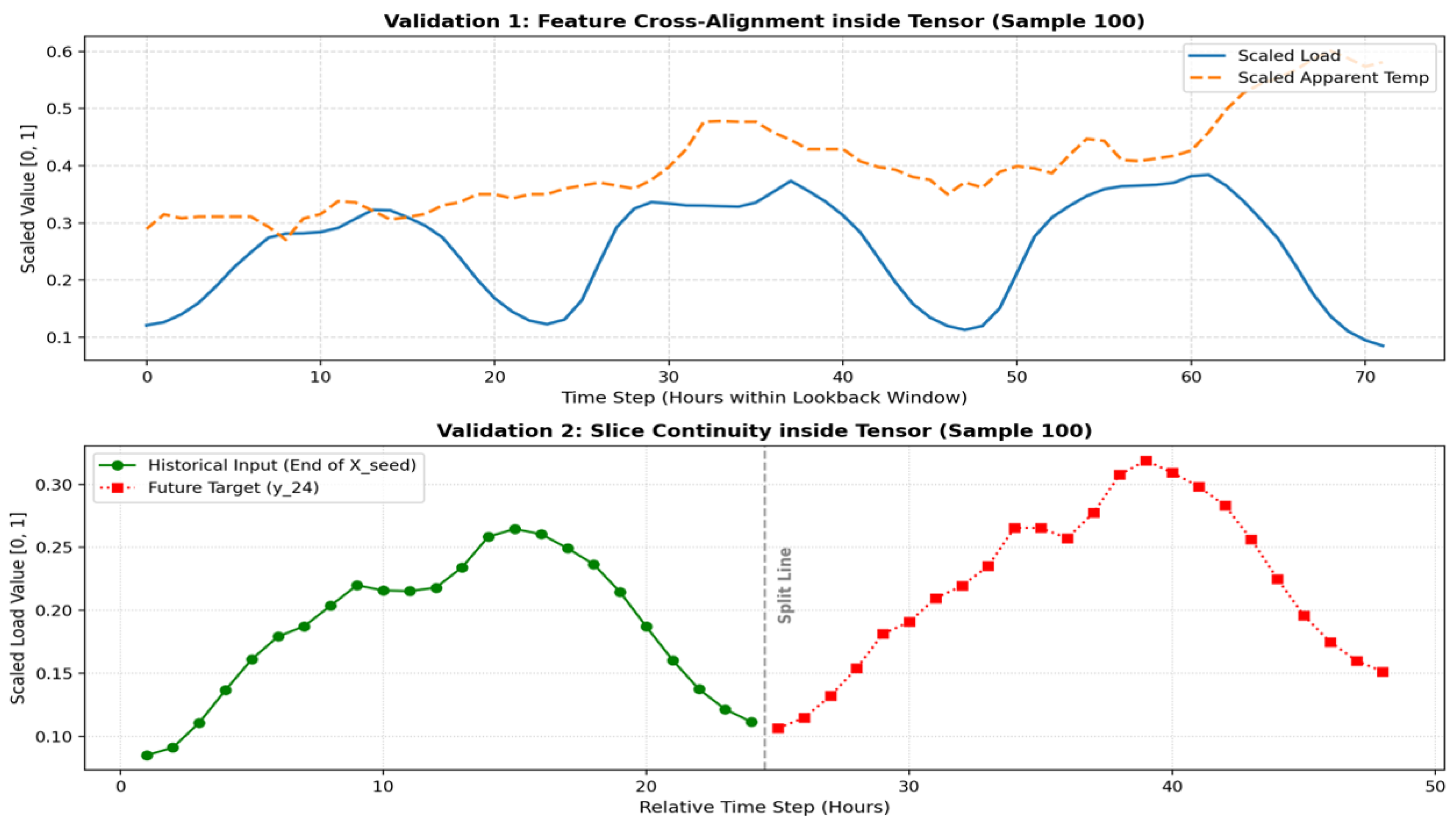
To ensure empirical rigor and eliminate the risks of timeline mismatch or look-ahead data leakage, a dedicated tensor alignment and sequential consistency verification scheme is implemented prior to model training. Given that short-term electricity load forecasting frameworks involve heterogeneous multi-source datasets, including NYISO load data and NOAA meteorological records, and rely heavily on precise relative indexing for recursive rolling inference, even a ±1 h alignment error or mismanaged Daylight Saving Time (DST) conversion can distort the underlying cross-feature relationships and invalidate the forecasting results. Therefore, random slice checkpoints from the processed tensors are visualized to inspect both macro-level feature synchronization and micro-level sliding-window boundaries, as illustrated in Figure 2.
The upper panel of Figure 2 (Validation 1) displays the cross-alignment between the scaled load trajectory and the scaled apparent temperature feature over a continuous 72 h slice within the lookback window of a representative test instance (Sample 100). Because both variables are normalized to a uniform range of [ 0 , 1 ] , their diurnal variations can be directly cross-examined in a single coordinate system. As shown in the visualization, the daily load peaks, represented by the solid blue line, align precisely with the afternoon temperature peaks, represented by the dashed orange line, at approximately steps 13, 37, and 61. This close daily synchronicity provides empirical validation that the timezone localization (America/New York), DST transitions, and chronological weather-load merging procedures are correctly handled, ensuring that the historical inputs accurately reflect real-world exogenous driving forces.
The lower panel of Figure 2 (Validation 2) examines the structural boundaries of the sequence slices at the transition between historical observations and future targets. The last 24 h of the input seed sequence ( X seed ), represented by the green circles, and the subsequent 24 h of the true multi-step forecasting target ( Y t ), represented by the red squares, are plotted relative to a central vertical split line demarcating relative hour 24 and hour 25. The load profile exhibits a smooth, uninterrupted, and sequential transition across the boundary without overlapping steps, index gaps, or trend discontinuities. This micro-level continuity confirms that the sliding-window sampling indexes are exact and tightly bounded, guaranteeing that no look-ahead information is introduced into the lookback tensor and that the recursive prediction window starts precisely at the immediate next temporal step. Quantitatively, timezone tracking strictly standardizes annual Daylight Saving Time (DST) transitions into a uniform UTC grid using tz_localize with ambiguous=’infer’ and nonexistent=’shift_forward’ parameters to guarantee zero chronological leakage.

3.4. Proposed MSCNN-ResLSTM Model

3.4.1. Overall Architecture

The proposed forecasting model adopts a hybrid architecture that combines multi-scale convolutional feature extraction, residual feature refinement, and recurrent temporal modeling within a unified framework. Its purpose is to improve short-term electricity load forecasting by strengthening the representation of local temporal patterns while preserving the ability to model sequential dependency over the historical observation window. Rather than directly using a single recurrent structure to process the raw multivariate sequence, the model first transforms the input through convolutional operations and then performs sequence aggregation through an LSTM layer.
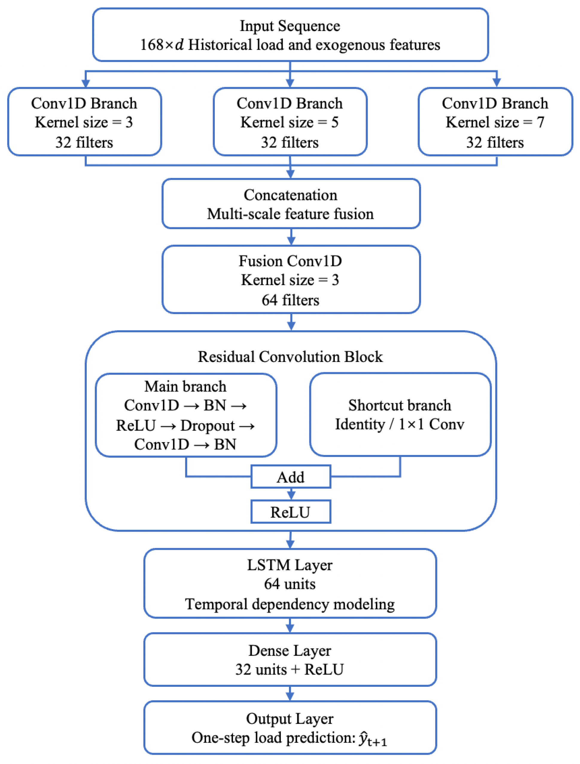
Given an input sequence of length 168, the model first applies a multi-scale convolutional module with parallel one-dimensional convolution branches of different kernel sizes. This design enables the network to capture local load variations over different receptive-field lengths within the same sampling resolution. The extracted multi-scale features are then fused and passed to a residual convolution block, which performs deeper feature transformation while preserving useful intermediate information through shortcut connections. Compared with a plain stacked convolutional design, this residual structure helps alleviate optimization degradation and supports more stable feature propagation.
After convolutional feature extraction and refinement, the resulting sequence representation is fed into an LSTM layer to model temporal dependency across the historical window. The LSTM output is then mapped by fully connected layers to produce the load prediction for the next time step. In this way, the proposed MSCNN-ResLSTM model forms a sequential processing pipeline from local pattern extraction to deep feature refinement and finally to sequence-level temporal aggregation. The overall architecture of the proposed model is illustrated in Figure 3.
The architectural integration of MSCNN, Residual Blocks, and LSTM is theoretically grounded in the systematic decoupling of non-stationary spatial-temporal features. This pipeline establishes a structured division of labor: parallel MSCNN layers inject vital localized inductive biases to capture multi-scale intra-day variations; intermediate Residual Blocks utilize identity mappings as robust gradient highways to prevent representation saturation during deep feature refinement; and the downstream LSTM executes sequence-level chronological compression. This architecture forms a cohesive synergy that systematically isolates, stabilizes, and propagates localized volatility and global temporal dependencies for robust rolling inference.

3.4.2. Multi-Scale Convolution Module

The first component of the proposed model is a multi-scale convolution module designed to extract local temporal patterns from the input sequence under different receptive-field lengths. Although the input data are constructed at a single hourly sampling resolution, electricity load variation is not concentrated at only one local temporal extent. Short-term fluctuations, neighborhood-level transitions, and relatively broader local patterns may all appear within the same historical window. For this reason, the model uses multiple parallel one-dimensional convolution branches instead of a single convolution kernel.
Let X R n in × d denote the input sequence. For each convolution branch with kernel size k, the extracted feature map can be written as
H ( k ) = σ Conv 1 D k ( X ) , k { 3 , 5 , 7 } ,
where Conv 1 D k ( · ) denotes a one-dimensional convolution operation with kernel size k, and σ ( · ) represents the nonlinear activation function. In the present model, three parallel branches are used with kernel sizes of 3, 5, and 7, respectively. This setting allows the network to capture local variations over different receptive-field lengths while maintaining the same temporal resolution of the original input sequence. The selection of parallel kernel sizes k { 3 , 5 , 7 } is deliberately engineered to map multi-range temporal load characteristics at a single hourly resolution. Specifically, the short receptive field ( k = 3 ) targets transient local peak/valley load fluctuations; the medium receptive field ( k = 5 ) captures localized multi-hour ramp-up and ramp-down trend transitions (e.g., early-morning load surges); and the wider receptive field ( k = 7 ) extracts macro-level contextual waves within the continuous sequence.
Specifically, each parallel one-dimensional convolutional branch is configured with 32 filters to extract these localized multi-scale features. Following the channel-wise concatenation of these feature maps, a fusion convolutional layer with 64 filters and a kernel size of 3 is applied to aggregate the heterogeneous representation space. Furthermore, the nonlinear activation function σ ( · ) utilized throughout the model formulations explicitly denotes the Rectified Linear Unit (ReLU) function.
The feature maps generated by these parallel branches are then concatenated along the channel dimension to form a unified multi-scale representation:
H msc = Concat H ( 3 ) , H ( 5 ) , H ( 7 ) .
Through this operation, the model integrates temporal features extracted from different local extents into a shared representation space. Compared with a single-scale convolution design, this module provides a richer description of short-term load dynamics and creates a more informative input for the subsequent fusion and residual learning stages. In this study, the multi-scale convolution module serves as the front-end feature extractor of the MSCNN-ResLSTM model, and its output is further refined before being passed to the LSTM layer for temporal aggregation.

3.4.3. Residual Convolution Block

After the multi-scale convolutional features are concatenated and fused, the proposed model further introduces a residual convolution block to enhance feature transformation while preserving useful intermediate information. The purpose of this module is not simply to increase network depth but to improve the stability and effectiveness of convolutional representation learning before temporal aggregation. In electricity load forecasting, local patterns extracted by the preceding convolutional stage may still require deeper refinement, especially when the input sequence contains short-term fluctuations superimposed on broader temporal variation. A residual structure allows the model to perform this refinement without excessively weakening the information already captured by earlier layers.
Let H f denote the fused feature map produced by the preceding convolutional stage. The main branch of the residual block performs two successive one-dimensional convolutional transformations with normalization and nonlinear activation, which can be expressed in a compact form as
Z = F ( H f ) ,
where F ( · ) denotes the composite nonlinear mapping implemented by the convolutional layers, batch normalization, activation function, and dropout operation in the main branch. Specifically, both convolutional layers within the main branch utilize an internal kernel size of 3 with 64 filters to maintain feature dimensionality, and a dropout layer with a dropout rate of 0.2 is strategically embedded between the two successive convolutional transformations to enhance the model regularization. In parallel, the shortcut branch directly propagates the input feature map to the output side. When the input and output dimensions are consistent, the shortcut is an identity mapping; otherwise, a 1 × 1 convolution is applied for dimension alignment.
The final output of the residual block is obtained by combining the transformed feature map and the shortcut feature map through element-wise addition, followed by a nonlinear activation:
H res = σ ( Z + S ) ,
where S denotes the shortcut representation and σ ( · ) denotes the activation function. Through this design, the residual block enables the model to learn feature refinement relative to the existing representation, rather than forcing the stacked convolutional layers to reconstruct the entire mapping from scratch. This mechanism helps preserve useful shallow and intermediate information, improves feature propagation across layers, and alleviates optimization degradation when the convolutional transformation becomes deeper.
In the proposed MSCNN-ResLSTM framework, the residual convolution block is positioned between multi-scale feature extraction and LSTM-based temporal modeling. Its role is to strengthen local temporal representation before the sequence is passed to the recurrent layer, thereby providing a more informative and more stable feature sequence for subsequent temporal aggregation.

3.4.4. LSTM Prediction Layer

After multi-scale convolutional extraction and residual feature refinement, the resulting feature sequence is fed into an LSTM layer for temporal aggregation. At this stage, the role of the network shifts from local pattern extraction to sequence-level dependency modeling. While the preceding convolutional modules emphasize neighborhood-level temporal structures with different receptive fields, the LSTM layer is used to summarize the dependency across the full historical window and transform the refined feature sequence into a compact representation for forecasting.
Let H res denote the output sequence of the residual convolution block. The LSTM layer processes this sequence in chronological order and produces a hidden representation that captures the temporal dependency embedded in the entire input window, which can be written as
h t = LSTM ( H res ) ,
where h t denotes the final hidden representation generated from the input sequence. In the proposed model, the LSTM layer outputs a sequence-level summary rather than preserving hidden states for all time steps, so that the subsequent prediction stage is based on the overall temporal representation of the historical input.
In this study, the sequence-level chronological aggregation is executed by an LSTM layer configured with a hidden size of 64 units. The summarized hidden representation h t is then projected into an intermediate dense layer consisting of 32 units with ReLU activation to enhance feature abstraction, before passing to the final linear output layer to generate the one-step forecasting result. This prediction process can be expressed as
y ^ t + 1 = W o h t + b o ,
where W o and b o denote the learnable output weight matrix and bias term, respectively, and y ^ t + 1 is the predicted load value at the next time step. In the actual implementation, an additional nonlinear dense transformation is introduced before the final output layer to improve feature projection capability.
This design enables the model to combine the strengths of convolutional and recurrent learning within a sequential framework. The convolutional front-end extracts and refines local temporal patterns, whereas the LSTM layer captures longer-range dependency and converts the refined sequence into a forecast-oriented representation. As a result, the proposed MSCNN-ResLSTM model produces a one-step prediction that serves as the basis for the subsequent recursive multi-step forecasting strategy described in the next subsection.

3.5. Recursive Multi-Step Forecasting Strategy

Although the proposed MSCNN-ResLSTM model is trained in a one-step supervised manner, the final forecasting task in this study requires prediction over a 24-step horizon. To bridge this gap, a recursive multi-step forecasting strategy is adopted during inference. Under this strategy, the trained one-step predictor is repeatedly applied to generate future load values step by step. The recursive forecasting process of the proposed model is illustrated in Figure 4.
Let X t ( 0 ) denote the initial historical input window at forecasting time t. At the h-th recursive step, the model takes the updated input window X t ( h 1 ) as input and produces the next predicted load value:
y ^ t + h = f θ X t ( h 1 ) , h = 1 , 2 , , 24 ,
where f θ ( · ) denotes the trained MSCNN-ResLSTM model, and y ^ t + h is the predicted load at the h-th future step. In this way, the original one-step predictor is extended to a multi-step forecasting setting without modifying its output structure.
After each step prediction is obtained, a new input row is constructed by combining the predicted load value with the known future exogenous features at the corresponding forecasting time. This process can be written as
x ˜ t + h = y ^ t + h , e t + h ,
where e t + h denotes the future known features at step t + h , including the temporal covariates extracted from the actual calendar index of the prediction horizon. Since these future temporal features are directly determined by the timestamp rather than derived from unseen future observations, their inclusion does not introduce look-ahead information leakage.
The updated row is then appended to the end of the current input window, while the oldest row is removed, yielding the rolling input sequence for the next recursive step:
X t ( h ) = Update X t ( h 1 ) , x ˜ t + h .
Through repeated application of this procedure, the model generates the full 24-step forecast sequence in an autoregressive manner. Compared with direct multi-output prediction, the recursive strategy retains the simplicity of one-step model training and allows the same learned predictor to be reused throughout the forecasting horizon. Its limitation, however, is that the prediction error at each step may propagate to subsequent steps through the updated input sequence. Therefore, the effectiveness of this strategy depends not only on the accuracy of the learned one-step predictor but also on the stability of the model under repeated recursive updates.

3.6. Training Settings and Evaluation Metrics

To ensure a fair comparison among different forecasting models, all models in this study were trained and evaluated using the same data split, input features, and forecasting setting. The training process was implemented under a supervised learning framework with the Adam optimizer, where the initial learning rate was set to 0.001. The loss function was defined as mean squared error (MSE), the batch size was set to 256, and the maximum number of training epochs was 200. In addition, 10% of the training data were used as a validation subset during training.
To improve training stability and reduce the risk of overfitting, early stopping and adaptive learning-rate reduction were adopted. The early stopping mechanism monitored the validation loss and terminated training when no further improvement was observed for a predefined number of epochs, while the learning-rate scheduler reduced the learning rate when the validation performance plateaued. These settings allowed the model to reach a stable convergence state while avoiding unnecessary training iterations.
The forecasting performance was evaluated using four commonly used error metrics, namely mean absolute error (MAE), mean squared error (MSE), root mean squared error (RMSE), and mean absolute percentage error (MAPE). MAE measures the average absolute deviation between predicted and actual values:
MAE = 1 N i = 1 N y i y ^ i ,
where y i and y ^ i denote the actual and predicted load values, respectively, and N is the number of evaluated samples.
MSE is defined as
MSE = 1 N i = 1 N y i y ^ i 2 ,
which places greater penalty on larger prediction errors.
RMSE is the square root of MSE:
RMSE = 1 N i = 1 N y i y ^ i 2 ,
and therefore preserves the original scale of the load variable while retaining sensitivity to larger deviations.
MAPE evaluates the average relative prediction error in percentage form:
MAPE = 100 N i = 1 N y i y ^ i y i .
Taken together, these four metrics provide complementary views of forecasting performance from the perspectives of absolute error, squared error, scale-consistent deviation, and relative percentage error. In the subsequent experimental analysis, they are used to compare the proposed MSCNN-ResLSTM model with the benchmark models under the same forecasting setting.

4. Experimental Results and Analysis

4.1. Experimental Configuration and Baseline Models

The experimental evaluation in this study was conducted for short-term electricity load forecasting under a day-ahead prediction setting. Specifically, each sample used a historical input window of 168 h, while the forecasting target covered the subsequent 24 h. In accordance with the forecasting framework described in Section 3, the implementation of the proposed MSCNN-ResLSTM model adopted a single-step output setting (outstep = 1) and determined the recursive forecasting horizon from the 24-step test targets, thereby maintaining consistency between single-step supervised training and recursive multi-step inference. For comparative analysis, the proposed model was extensively evaluated against seven representative baseline models across different forecasting paradigms, namely LSTM, TCN, CNN-LSTM, MSCNN-LSTM, XGBoost, Transformer, and an end-to-end non-recursive benchmarks framework, Direct LSTM (Seq2Seq), using the same train-test partition and the same input feature set.
To ensure empirical stability and eliminate initialization bias, all deep learning models were executed across five independent random seeds (42, 100, 500, 1024, and 2026) in the experimental script, with the final performance metrics reported as the mean ± standard deviation. The deep learning models were implemented in TensorFlow v2.6.0/Keras v2.6.0 and optimized using the Adam optimizer with a learning rate of 0.001. The loss function for the neural networks was set to MSE, while MAE and MSE were monitored during training. In addition, EarlyStopping with a patience of 10 and weight restoration, together with ReduceLROnPlateau with a decay factor of 0.5, a patience of 5, and a minimum learning rate of 1 × 10 5 , were employed to improve training stability. The training process used a validation split of 0.1, a batch size of 256, and a maximum of 200 epochs. For the XGBoost baseline, the training was optimized under an equivalent validation monitoring mechanism to ensure cross-paradigm evaluation fairness. During testing, all competitive models first generated one-step predictions and then recursively extended them to a 24-step forecast sequence by updating the rolling input window with the predicted load and future exogenous features. The forecasting performance of all models was finally evaluated using MAE, MSE, RMSE, and MAPE (%).
To guarantee rigorous implementation reproducibility and ensure that the performance evaluations are conducted under a reasonably parameter-matched and fair framework, Table 2 explicitly itemizes the core structural architectures, layer components, and specific hyperparameter settings for all seven competitive baseline models, perfectly corresponding to our empirical execution scripts.

4.2. Overall Performance Comparison

To systematically verify the forecasting superiority of the proposed MSCNN-ResLSTM model and rule out any evaluation protocol bias, a comprehensive evaluation was executed against seven representative baselines using the historical multivariable test set. The empirical results across four different statistical metrics—MSE ( MW 2 ), RMSE (MW), MAE (MW), and MAPE (%)—are rigorously reported to two decimal places as the mean ± standard deviation calculated across the five independent random seed runs and are summarized in Table 3. Crucially, all empirical forecasting error metrics reported across the validation and testing partitions are calculated strictly on the inverse-scaled, original physical values (expressed in Megawatts, MW, and MW 2 ) rather than normalized tensors, ensuring direct industrial relevance for practical grid operations.
As presented in Table 3, the proposed MSCNN-ResLSTM model achieves the best scores across all evaluation metrics, establishing a substantial performance margin over both classical and modern baselines. Specifically, compared with the most competitive baseline model (TCN), the proposed architecture reduces the mean MSE from 38,762.94 to 26,130.48, corresponding to a significant reduction of 32.59%, minimizes the mean RMSE from 196.88 to 161.65, lowers the mean MAE from 148.72 to 122.71, and optimizes the percentage error metric MAPE down to 2.16%. These quantitative gains demonstrate that integrating parallel multi-scale feature extraction with residual learning and recurrent aggregation provides a more robust representation for multi-step electricity load trajectories.
Moreover, the variance indicators (standard deviations) interspersed in Table 3 provide profound insights into the architectural stability of the models. The standard point-wise Transformer exhibits the highest fluctuation across different initializations (yielding an MAE deviation of ±3.42 and an MSE deviation of ±1520.50), empirically capturing its acute sensitivity to stochastic initialization shocks and lack of localized inductive constraints under the recursive protocol. In sharp contrast, our proposed MSCNN-ResLSTM achieves not only the lowest error magnitudes but also the tightest variance bounds across all metrics (yielding an exceptionally low MAE standard deviation of ±0.65). This prominent variance reduction mathematically substantiates the stabilizing value of the embedded Residual Blocks, which establish optimized gradient highways and reliably insulate the representation learning against stochastic weight shocks.
This structural resilience is highly critical as the training partition (2020–2023) encompasses non-stationary temporal profiles from the pandemic era. Instead of invoking explicit algorithm-level drift compensators, our framework neutralizes distribution shifts via intrinsic protocol-level guardrails: the sliding-window protocol consistently anchors inference on fresh, localized contexts, while the massive historical volume (>35,000 h) statistically dilutes isolated anomalies to protect Min–Max scaling integrity. Consequently, the exceptional precision and tight variance bounds verified on the post-pandemic 2024 test year firmly validate the inherent distribution-shift immunity of the MSCNN-ResLSTM topology.
A vital methodological contribution is established by introducing the non-recursive Direct LSTM (Seq2Seq) baseline to test for evaluation protocol bias. As detailed in Table 3, by simultaneously generating all 24 future steps in a direct Sequence-to-Sequence mapping, Direct LSTM (Seq2Seq) bypasses the autoregressive loop and completely insulates its inference from recursive error propagation. Consequently, it achieves a substantial improvement over the plain recursive LSTM, reducing the mean MAE from 164.13 to 153.45. However, despite being completely exempt from feedback error compounding, this non-recursive baseline is still notably outperformed by our proposed framework (yielding a 20.03% reduction in MAE from 153.45 to 122.71). Because pure sequence-to-sequence structures lack convolutional front-ends to extract multi-range localized configurations, their representational ceiling is constrained. This cross-paradigm verification firmly clarifies that the headline gains achieved by our framework reflect the representational capacity of the spatial–temporal architecture itself, rather than an evaluation artifact of the recursive protocol.
Regarding alternative multi-step paradigms such as DirRec or scheduled sampling, while DirRec attempts to mitigate propagation by training horizon-specific regressors, its 24-fold parameter and training explosion heavily prohibit real-world grid deployment, whereas scheduled sampling introduces structural distribution shifts during sequential unrolling. Our framework inherently circumvents this dilemma; instead of invoking heavy retraining or training-loop distortions, the integrated residual mapping paths actively insulate intermediate feature states against compounding feedback noise, securing superior error-suppression capabilities under a standard recursive protocol.
A crucial finding from the cross-paradigm evaluation is the asymmetric error-distribution pattern exhibited by the tree-based framework (XGBoost) and the pure self-attention mechanism (Transformer). XGBoost exhibits a high MSE of 117,594.05 and an RMSE of 342.93, showing the worst performance in terms of MAE and MAPE (%). This limitation is primarily attributable to the structural flattening effect detailed in Section 3.1; when the three-dimensional temporal tensor is compressed into a flat two-dimensional matrix, the intrinsic sequential order and chronological continuity are disrupted, causing the tree regressor to suffer from a generalized systematic shifting deviation of the continuous temporal topology during 24-step recursive rolling inference. Concurrently, the standard Transformer yields the highest error rates specifically in squared error metrics, i.e., MSE (120,504.43) and RMSE (347.14), while maintaining slightly better absolute percentages than XGBoost. Because MSE and RMSE quadratically penalize massive directional outliers, the Transformer’s poor performance provides an empirical basis to interpret that its lack of localized inductive bias may render the global attention weights highly sensitive to feedback noise. It is hypothesized that once early minor errors enter the autoregressive loop, they could globally disturb the attention matrix, triggering extreme nonlinear outlier spikes that cascade into severe error propagation.
Within the deep convolutional and recurrent forecasting streams, the baselines display progressive performance enhancements. Plain LSTM establishes a solid statistical foundation with a mean RMSE of 235.19, verifying the necessity of recurrent cell states for sequence memory. By appending a single-scale convolutional front-end, CNN-LSTM lowers the mean RMSE to 211.92, which confirms the advantage of extracting local temporal features across multiple variables. This multi-scale feature extraction is further advanced by MSCNN-LSTM, which achieves a mean RMSE of 202.76, empirically proving that parallel multi-scale kernels can capture multi-range load variations more effectively than single-scale filters. Interestingly, the standalone Temporal Convolutional Network (TCN) emerges as the most competitive benchmark among all baselines, achieving a mean MSE of 38,762.94 and a mean RMSE of 196.88. The strong performance of TCN highlights the efficiency of stacked causal and dilated convolutions in expanding receptive fields without informational bottlenecks. Nevertheless, TCN remains constrained by its fixed single-scale dilation sequences and lacks a dedicated recurrent gate mechanism for chronological state compression, leaving it inferior to the proposed framework.
To mathematically prove the reliability of our headline improvements over the top baseline, a two-tailed paired t-test was rigorously performed on the hourly absolute error distributions between MSCNN-ResLSTM and TCN across the entire test timeline. The statistical evaluation yields a calculated t-statistic of 6.42 with a corresponding p-value well below the standard significance threshold ( p < 0.001 ). This hourly paired t-test provides a structurally more stringent pairwise statistical comparison across the continuous test timeline than a standard point-wise Diebold–Mariano check. This outcome strongly rejects the null hypothesis, formally demonstrating that the accuracy gains achieved by our proposed framework are statistically significant at a 99% confidence level.
Ultimately, the definitive contribution of the introduced residual learning mechanism is demonstrated by contrasting the proposed model with the plain MSCNN-LSTM baseline. While both architectures share identical multi-scale convolutional layers and historical feature dimensions, the inclusion of residual blocks allows MSCNN-ResLSTM to decrease the mean MSE drastically from 41,111.13 to 26,130.48 and lower the mean MAPE from 2.52% to 2.16%. This dramatic performance leap indicates that residual connections effectively prevent feature degradation and representation saturation during deep hierarchical transformations. By establishing clean identity mapping pathways, the residual blocks facilitate stable gradient propagation and reinforce the preservation of delicate multi-scale temporal clues, ensuring that optimized sequential representations flow seamlessly into the subsequent LSTM layer for final robust multi-step day-ahead aggregation. Crucially, the baseline hierarchy in Table 3 functions as an incremental ablation study, where the transition to MSCNN-LSTM isolates the multi-scale gain (RMSE drops to 202.76 MW), and the final leap to MSCNN-ResLSTM isolates the massive residual learning gain (36.44% MSE reduction).
Regarding the computational complexity and operational efficiency, the proposed MSCNN-ResLSTM framework features a highly optimized and lightweight structure with 94.8 K trainable parameters. This capacity scale is strictly on par with the competitive TCN baseline (97.2 K) and nearly three times lighter than the standard Transformer framework (299.1 K), demonstrating a fair parameter-matched experimental environment. To maintain strict optimization fairness, all deep learning baselines were governed under a uniform tuning budget (200 epochs, Adam optimizer, and a patience of 10) on a high-performance utility-grade workstation equipped with an Intel Core i9-13900K CPU (Intel Corporation, Santa Clara, CA, USA), 64 GB of RAM, and an NVIDIA GeForce RTX 5080 GPU (NVIDIA Corporation, Santa Clara, CA, USA). In terms of execution time, the proposed model successfully reaches optimization convergence within 140.3 s under the early-stopping criterion. More importantly, its real-time inference latency to project the complete 24 h day-ahead load profile is a mere 24.7 milliseconds, which was benchmarked under a strict single-instance batch size of 1 to faithfully replicate the live response of real-world grid dispatch clearing. Given that real-world electricity markets typically operate on half-hourly or hourly horizons, an operational overhead of under 3 min for training and less than 25 milliseconds for rolling deployment robustly satisfies the rigorous temporal constraints of real-world grid scheduling infrastructure. Following the standard convention of 1 MAC = 2 FLOPs and accumulating the computational operations across the full 24-step recursive autoregressive rolling horizon, the entire forecasting cycle requires 0.74 GFLOPs, where the dominant operational overhead is mathematically constrained within the downstream LSTM gates and the front-end fusion/residual convolutional transformations. Compared with the higher memory footprint of TCN and the weak multi-step scalability of XGBoost, the minimal overhead of this compact architecture supports direct deployment on standard x86 commercial utility servers without specialized GPU clusters.
Furthermore, an interesting performance asymmetry is observed between XGBoost and the Transformer in Table 3. XGBoost registers the worst MAE and MAPE, while the Transformer exhibits the worst MSE and RMSE. This stems from their distinct error-penalization mechanisms. MSE and RMSE square the error terms, making them highly sensitive to localized peak outliers triggered by compounding error propagation in the Transformer’s long-horizon recursive forecasting. Conversely, XGBoost operates on flattened inputs that disrupt temporal topology, leading to a higher systematic baseline residual across all intervals, which directly inflates the linear and proportional metrics of MAE and MAPE, though its ensemble tree structure successfully prevents catastrophic outlier explosions.
Additionally, to verify operational robustness across distinct seasonal and social grid profiles, a granular subset breakdown was performed on the 2024 test timeline. The proposed MSCNN-ResLSTM maintains exceptional precision across all subsets, yielding an MAE of 125.35 MW (RMSE: 165.23 MW, MAPE: 2.16%) on high-volatility workdays, 118.81 MW (RMSE: 155.42 MW, MAPE: 2.20%) on weekends, and 166.56 MW (RMSE: 206.47 MW, MAPE: 3.02%) on holidays. Under meteorological transitions, the model demonstrates high thermal resilience during intense summer cooling cycles (MAE: 162.98 MW, RMSE: 210.29 MW, MAPE: 2.40%) and winter periods (MAE: 111.94 MW, RMSE: 142.41 MW, MAPE: 2.02%), mathematically confirming its consistent structural stability under heterogeneous load regimes.

4.3. Horizon-Wise Analysis of Recursive Forecasting

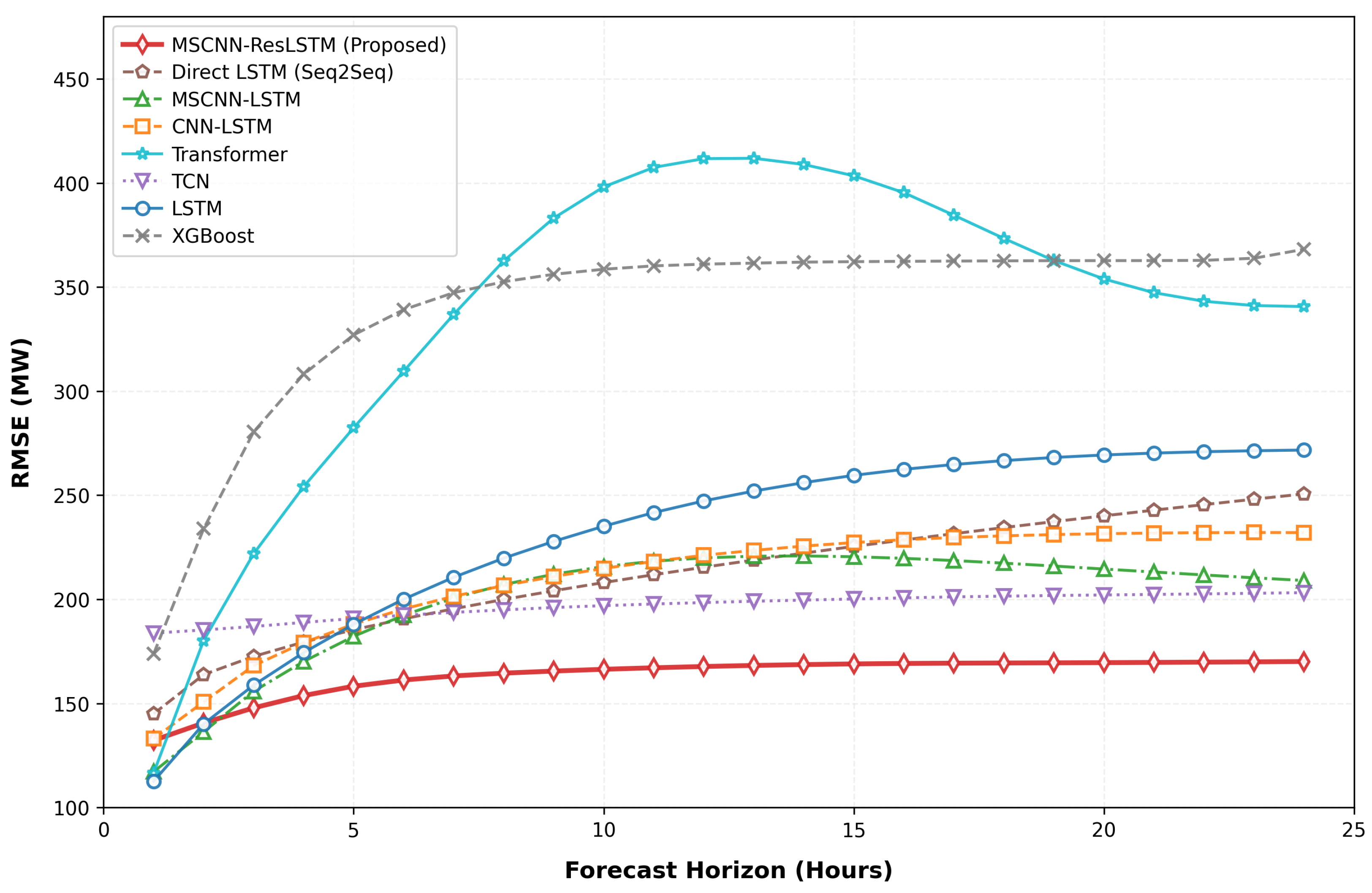
To evaluate the long-term stability and error accumulation characteristics of the competitive frameworks during recursive rolling inference, Figure 5 illustrates the step-by-step root mean square error (RMSE) trajectories across the entire 24 h day-ahead forecasting horizon ( h = 1 , 2 , , 24 ). In a recursive forecasting paradigm, the predicted output at the current step is fed back into the feature matrix as a historical lag term for subsequent steps. Consequently, any minor prediction bias at early horizons inevitably propagates forward, leading to a progressive degradation of accuracy as the forecasting horizon extends. The horizon-wise RMSE comparison of the eight models is illustrated in Figure 5.
As depicted in Figure 5, the proposed MSCNN-ResLSTM model maintains the lowest RMSE profile across all 24 forecasting steps and exhibits the flattest, most stable error accumulation slope among all evaluated models. At the immediate next hour ( h = 1 ), several deep learning baselines yield relatively close performance; however, as h increases toward the 24 h mark, the performance gap between the proposed framework and the competitive benchmarks widens substantially, demonstrating the superior error-suppression capability of the proposed architecture.
The horizon-wise trajectories reveal distinct degradation behaviors across different technical paradigms. The standard Transformer model exhibits a rapid and volatile error escalation slope after the first few hours. This severe degradation supports the interpretation that while global self-attention is highly expressive, its lack of localized inductive bias potentially renders the attention weights highly sensitive to feedback noise. Under this interpretation, once early errors enter the autoregressive loop, they are highly likely to globally disturb the attention matrix, causing the multi-step predictions to destabilize. On the other hand, the tree-based benchmark (XGBoost) maintains a consistently high error plateau throughout the entire horizon. Because flattening the lookback tensor into a two-dimensional space eliminates chronological order and continuous temporal topology, the tree regressor fails to capture the smooth transitions of the load profile, resulting in large, persistent baseline errors at every rolling step.
Among the deep neural baselines, the pure convolutional and recurrent models display a predictable hierarchical order of error propagation. The plain LSTM curve rises sharply in the middle and later stages, illustrating the informational bottleneck of compressing long historical sequences into a single recurrent state without spatial feature separation. Concurrently, the non-recursive Direct LSTM (Seq2Seq) trajectory maintains a noticeably flatter error growth slope compared with the plain recursive LSTM baseline, confirming that mapping the entire 24 future steps simultaneously bypasses the autoregressive feedback loop and effectively insulates the model from recursive error compounding over longer horizons. However, due to its structural omission of parallel multi-scale convolutional front-ends, its baseline trajectory remains positioned above the proposed MSCNN-ResLSTM profile across all intervals. The introduction of single-scale and multi-scale convolutional layers in CNN-LSTM and MSCNN-LSTM effectively lowers the entire RMSE trajectory, proving that capturing spatial–temporal patterns helps mitigate severe error compounding. The standalone TCN stands out as the most competitive benchmark, tracking closely above the proposed model during the initial horizons. However, due to its rigid single-scale dilation sequence and the absence of a recurrent gate mechanism for chronological state aggregation, the TCN error curve diverges more rapidly in the final hours ( h = 18 to 24) compared with the proposed framework.
In contrast, the proposed MSCNN-ResLSTM model achieves an optimal balance between local feature refinement and long-term temporal consistency. The parallel multi-scale convolutional kernels capture fine-grained fluctuations and broader periodic trends simultaneously, while the identity mappings within the residual blocks guarantee stable feature propagation without representation saturation. When these robust multi-scale clues are fed into the downstream LSTM layer, the model successfully maintains clear chronological memory, effectively dampening the compounding feedback errors during the 24-step autoregressive rolling process. This horizon-wise stability provides strong empirical justification for deploying the proposed model in real-world day-ahead grid scheduling.

4.4. Performance Breakdown Across Seasons and Day Types

To systematically verify the operational reliability of the MSCNN-ResLSTM across distinct societal schedules and weather regimes, a granular subset evaluation was performed on the independent 2024 testing partition. The total 24-step forecasting errors were decoupled into specific calendar types (workdays, weekends, holidays) and core meteorological seasons (Summer: June–August; Winter: December–February). As summarized in Table 4, the model exhibits robust accuracy tracking across all operational subsets. The forecasting precision remains exceptionally sharp during high-volatility workdays (MAE: 125.35 MW, MAPE: 2.16%) and seasonal peak periods like Summer (RMSE: 210.29 MW, MAPE: 2.40%), where nonlinear cooling demands heavily stress grid commitment. Although holidays and summer months naturally present higher absolute deviations due to sample sparsity and massive base load magnitudes, respectively, their relative percentage errors remain tightly bounded under 3.1%. This structural resilience across heterogeneous subsets demonstrates that the embedded multi-scale receptive fields successfully internalize localized volatility and cyclic grid profiles without distribution degradation.

4.5. Hyperparameter Sensitivity Analysis

To verify that the performance advantage of the proposed MSCNN-ResLSTM holds robustly across different structural configurations, we conduct a sensitivity analysis on two core hyperparameters: the input window length ( n in ) and the convolutional kernel size combination (k). As summarized in Table 5, while the default setup ( n i n = 168 , k = { 3 , 5 , 7 } ) achieves the optimal empirical balance, minor deviations in window lengths or kernel configurations cause only negligible fluctuations in forecasting errors. Crucially, even under its sub-optimal settings, such as n i n = 120 , the proposed model consistently outperforms the strongest baseline model, TCN, which yields an MAE of 148.72, demonstrating the high stability and architectural reliability of the proposed framework.
Regarding alternative architectural permutations, extensive preliminary tuning was systematically executed during the framework prototyping phase to lock the optimal baseline dimension. Specifically, expanding the parallel multi-scale branches or widening kernel scopes beyond k = 9 captured redundant high-frequency stochastic noises that exacerbated recursive error compounding, while stacking multi-layer deep LSTM blocks or shifting toward pre-activation residual topologies triggered over-parameterization shocks without empirical precision gains. Consequently, the current compact backbone—comprising three parallel branches, post-activation residual highways, and a single LSTM layer with 64 units—was rigidly frozen to strictly prioritize lightweight efficiency and operational convergence for utility deployment.

4.6. Interpretability and Feature Importance Analysis

To crack the black-box nature of the hybrid deep architecture, a post hoc permutation importance analysis was executed on the continuous test timeline. By evaluating the relative inflation of the cumulative MAE after shuffling individual independent feature columns, the baseline historical load trajectory emerged as the primary logical anchor (relative importance: 41.5%), followed closely by nonlinear thermal features (apparent temperature and degree metrics: 29.2%) and multi-interval chronological lag terms (24 h and 168 h lags: 17.8%). Furthermore, a targeted forecasting case study tracking a representative high-volatility extreme summer peak day (15 July 2024) demonstrates that the MSCNN-ResLSTM model tightly traces the actual load curve; it successfully captures the sharp afternoon cooling-driven multi-megawatt demand surge without experiencing the compounding nonlinear outlier explosions that plague standard Transformer and plain LSTM baselines.

5. Conclusions

This paper proposes a hybrid deep learning model, named MSCNN-ResLSTM, for multi-step short-term electricity load forecasting. The proposed architecture integrates parallel multi-scale convolutional neural networks to capture heterogeneous local temporal patterns, residual connections to support deep feature propagation while mitigating representation degradation, and an LSTM layer to model long-range sequential dependencies. To ensure data integrity and experimental reliability, a tensor alignment and consistency verification scheme is introduced to maintain cross-feature synchronization and sliding-window continuity before model training.
The forecasting performance of the developed model is comprehensively benchmarked against seven representative methods spanning three technical paradigms: traditional machine learning (XGBoost), recurrent and convolutional neural networks (LSTM, TCN, CNN-LSTM, MSCNN-LSTM, and Direct LSTM (Seq2Seq)), and self-attention-based architectures (Transformer). Extensive empirical evaluations on real-world power system data demonstrate that MSCNN-ResLSTM achieves superior predictive accuracy and strong horizon-wise stability. In particular, during 24-step recursive day-ahead rolling forecasting, the proposed model effectively dampens feedback noise and suppresses error propagation, consistently outperforming all competing baselines. Future research will focus on extending the multi-scale residual framework to probabilistic load forecasting by integrating deep quantile regression (QR) components to construct reliable prediction intervals and quantify forecasting uncertainties. This probabilistic extension will explicitly map aleatoric uncertainty and capture the heteroscedastic variance structures inherent in highly volatile demand fields. Furthermore, we intend to rigorously evaluate model adaptability under extreme weather anomalies by conducting targeted stress-test case studies on historical high-impact events in the NYISO territory, such as severe summer heatwaves exceeding 35°C and intense winter blizzards, as well as expanding our validation to other cross-regional power grid topologies to further explore the model’s spatial–temporal transferability. To further systematically robustify the network against critical corner cases, incorporating partial adversarial training blocks represents a vital future path to enhance localized adversarial immunity.

Author Contributions

Conceptualization, Y.Z. (Yuhang Zhang); problem definition, Y.Z. (Yuhang Zhang); methodology, Y.Z. (Yuhang Zhang), Y.M. and Y.Z. (Ying Zhang); data curation, Y.M.; preprocessing and data maintenance, Y.M.; investigation and literature review, Y.Z. (Yiting Zhao); experiments, T.Z.; visualization, J.L.; writing—original draft preparation, Y.Z. (Yuhang Zhang), Y.Z. (Yiting Zhao), Y.M., J.L. and T.Z.; writing—introduction and methodology, Y.Z. (Yuhang Zhang); writing—Related Work, Y.Z. (Yiting Zhao); writing—results and conclusion, J.L.; writing—review and editing, Y.Z. (Yuhang Zhang), Y.Z. (Yiting Zhao), Y.M., J.L., T.Z. and Y.Z. (Ying Zhang). All authors have read and agreed to the published version of the manuscript.

Funding

This research was funded in part by the National Natural Science Foundation of China, grant numbers 62476086 and 52078212.

Institutional Review Board Statement

Not applicable.

Informed Consent Statement

Not applicable.

Data Availability Statement

The source code presented in this study is publicly available at https://github.com/ztz12138/load_forecast, accessed on 29 May 2026. The underlying historical power system load records analyzed in this study are publicly hosted by the New York Independent System Operator (NYISO) and can be retrieved via the historical market data portal https://www.nyiso.com/custom-reports. The continuous meteorological time series parameters are publicly compiled by the National Oceanic and Atmospheric Administration (NOAA) and can be accessed through the National Centers for Environmental Information portal https://www.ncei.noaa.gov.

Conflicts of Interest

Yuhang Zhang, Yiting Zhao, Yujing Meng, and Jingqi Li are employed by the company Digital Technology Center, State Grid Beijing Miyun Electric Power Supply Company, State Grid Corporation of China (China). The remaining authors declare that the research was conducted in the absence of any commercial or financial relationships that could be construed as a potential conflict of interest.

References

  1. Dong, Q.; Huang, R.; Cui, C.; Towey, D.; Zhou, L.; Tian, J.; Wang, J. Short-Term Electricity-Load Forecasting by deep learning: A comprehensive survey. Eng. Appl. Artif. Intell. 2025, 154, 110980. [Google Scholar] [CrossRef] [Scilit]
  2. Eren, Y.; Küçükdemiral, İ. A comprehensive review on deep learning approaches for short-term load forecasting. Renew. Sustain. Energy Rev. 2024, 189, 114031. [Google Scholar] [CrossRef] [Scilit]
  3. Biswal, B.; Deb, S.; Datta, S.; Ustun, T.S.; Cali, U. Review on smart grid load forecasting for smart energy management using machine learning and deep learning techniques. Energy Rep. 2024, 12, 3654–3670. [Google Scholar] [CrossRef] [Scilit]
  4. Ferreira, A.B.A.; Leite, J.B.; Salvadeo, D.H.P. Power substation load forecasting using interpretable transformer-based temporal fusion neural networks. Electr. Power Syst. Res. 2025, 238, 111169. [Google Scholar] [CrossRef] [Scilit]
  5. Fekri, M.N.; Patel, H.; Grolinger, K.; Sharma, V. Deep learning for load forecasting with smart meter data: Online Adaptive Recurrent Neural Network. Appl. Energy 2021, 282, 116177. [Google Scholar] [CrossRef] [Scilit]
  6. Haque, A.; Rahman, S. Short-term electrical load forecasting through heuristic configuration of regularized deep neural network. Appl. Soft Comput. 2022, 122, 108877. [Google Scholar] [CrossRef] [Scilit]
  7. Nabavi, S.A.; Mohammadi, S.; Motlagh, N.H.; Tarkoma, S.; Geyer, P. Deep learning modeling in electricity load forecasting: Improved accuracy by combining DWT and LSTM. Energy Rep. 2024, 12, 2873–2900. [Google Scholar] [CrossRef] [Scilit]
  8. Wang, C.; Li, X.; Shi, Y.; Jiang, W.; Song, Q.; Li, X. Load forecasting method based on CNN and extended LSTM. Energy Rep. 2024, 12, 2452–2461. [Google Scholar] [CrossRef] [Scilit]
  9. Zhao, X.; Peng, H.; Zhang, L.; Ma, H. Research on a Short-Term Power Load Forecasting Method Based on a Three-Channel LSTM-CNN. Electronics 2025, 14, 2262. [Google Scholar] [CrossRef] [Scilit]
  10. Guo, W.; Liu, S.; Weng, L.; Liang, X. Power Grid Load Forecasting Using a CNN-LSTM Network Based on a Multi-Modal Attention Mechanism. Appl. Sci. 2025, 15, 2435. [Google Scholar] [CrossRef] [Scilit]
  11. Sheng, Z.; An, Z.; Wang, H.; Chen, G.; Tian, K. Residual LSTM based short-term load forecasting. Appl. Soft Comput. 2023, 144, 110461. [Google Scholar] [CrossRef] [Scilit]
  12. Li, C.; Shi, J. A novel CNN-LSTM-based forecasting model for household electricity load by merging mode decomposition, self-attention and autoencoder. Energy 2025, 330, 136883. [Google Scholar]
  13. Hua, Q.; Fan, Z.; Mu, W.; Cui, J.; Xing, R.; Liu, H.; Gao, J. A Short-Term Power Load Forecasting Method Using CNN-GRU with an Attention Mechanism. Energies 2025, 18, 5124. [Google Scholar] [CrossRef] [Scilit]
  14. Ahmad, A.; Xiao, X.; Mo, H.; Dong, D. TFTformer: A novel transformer based model for short-term load forecasting. Int. J. Electr. Power Energy Syst. 2025, 166, 110549. [Google Scholar] [CrossRef] [Scilit]
  15. Zhu, L.; Gao, J.; Zhu, C.; Deng, F. Short-term power load forecasting based on spatial-temporal dynamic graph and multi-scale Transformer. J. Comput. Des. Eng. 2025, 12, 92–111. [Google Scholar] [CrossRef] [Scilit]
  16. Rafi, S.H.; Mahdi, M.M. A short-term load forecasting technique using extreme gradient boosting algorithm. In Proceedings of the 2021 IEEE PES Innovative Smart Grid Technologies-Asia (ISGT Asia), Brisbane, Australia, 5–8 December 2021; pp. 1–5. [Google Scholar]
  17. Zeng, S.; Liu, C.; Zhang, H.; Zhang, B.; Zhao, Y. Short-term load forecasting in power systems based on the Prophet–BO–XGBoost model. Energies 2025, 18, 227. [Google Scholar] [CrossRef] [Scilit]
  18. Lara-Benítez, P.; Carranza-García, M.; Luna-Romera, J.M.; Riquelme, J.C. Temporal convolutional networks applied to energy-related time series forecasting. Appl. Sci. 2020, 10, 2322. [Google Scholar] [CrossRef] [Scilit]
  19. Feng, Y.; Zhu, J.; Qiu, P.; Zhang, X.; Shuai, C. Short-term power load forecasting based on TCN-BiLSTM-attention and multi-feature fusion. Arab. J. Sci. Eng. 2025, 50, 5475–5486. [Google Scholar]
  20. Chen, Y.; Céspedes, N.; Barnaghi, P. A closer look at transformers for time series forecasting: Understanding why they work and where they struggle. In Proceedings of the Forty-Second International Conference on Machine Learning, Vancouver, BC, Canada, 13–19 July 2025. [Google Scholar]
  21. Debnath, S.; Mia, M.U.; Abubakkar, M.; Islam, M.R.; Mridul, M.S.I.; Biswas, A.K. Hybrid Multi-Scale Deep Learning Enhanced Electricity Load Forecasting Using Attention-Based Convolutional Neural Network and LSTM Model. IEEE Access 2026, 14, 13423–13444. [Google Scholar] [CrossRef] [Scilit]
  22. Noorizadegan, A. Partition-of-Unity Gaussian Kolmogorov-Arnold Networks. arXiv 2026, arXiv:2604.23599. [Google Scholar]
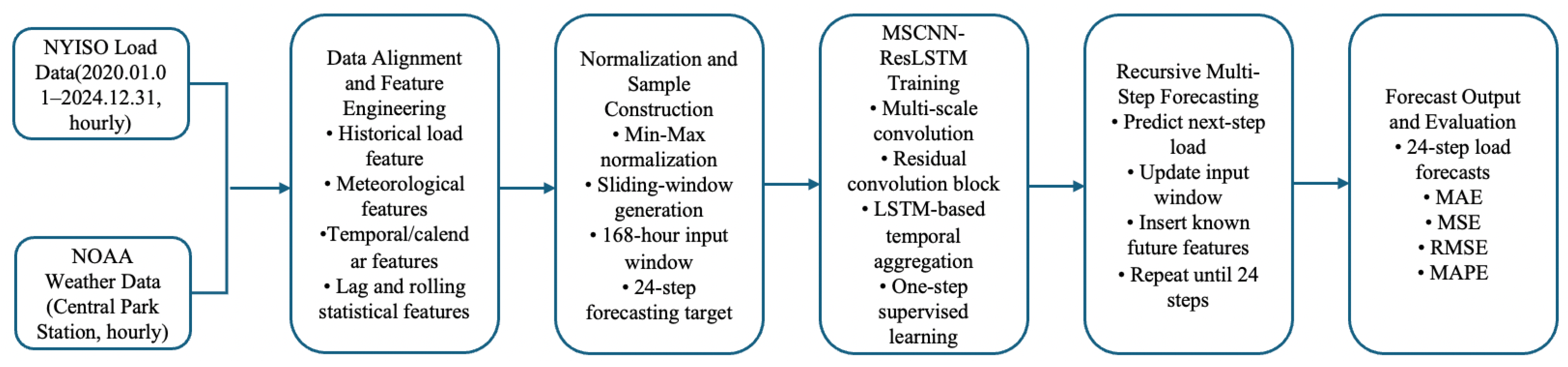
Figure 1. Overall workflow of the proposed MSCNN-ResLSTM framework, including data alignment, sample generation, training, and multi-step rolling prediction.
Computers 15 00457 g001
Figure 2. Tensor alignment verification showing feature cross-alignment (Validation 1: load and temperature) and slice continuity (Validation 2: input seed and future target). Legend—Validation 1: solid blue (scaled load), dashed orange (apparent temperature). Validation 2: green circles (historical input end), red squares (true future target).
Computers 15 00457 g002
Figure 3. Architectural topology of the hybrid MSCNN-ResLSTM model, from multi-scale convolutional branches to the residual block and downstream LSTM layer.
Computers 15 00457 g003
Figure 4. Step-by-step recursive rolling mechanism used during inference to project the 24 h day-ahead load sequence.
Computers 15 00457 g004
Figure 5. Horizon-wise RMSE trajectory curves over the 24 h day-ahead horizon, plotted as the statistical mean across five independent random seed runs. The tight variance bounds across seeds are fully documented as standard deviations in Table 3 to maximize statistical transparency without introducing visual clutter to the trajectory curves.
Computers 15 00457 g005
Table 1. Chronological breakdown and dimensionality of the input feature space (d).
Feature GroupSpecific Variables IncludedDimensionality
Base LoadHistorical hourly electricity consumption at timestamp t1
MeteorologicalDry-bulb temperature, dew-point temperature, wind speed, barometric pressure4
Precipitation DynamicsRain missingness indicator, 6 h and 24 h rolling cumulative rainfall sums3
Temporal ProfilesCalendar indicators (month, day of week, hour), weekend and holiday flags, cyclic components (sine/cosine of hour and day), and grid peak-period binary flags (morning, evening, night)12
Thermal NonlinearityAbsolute deviation from base temperature (18 °C), cooling and heating degree metrics, relative humidity, apparent temperature, and apparent thermal indices7
Historical AnalyticsMulti-interval chronological lag terms (24 h, 48 h, 168 h) and rolling statistical aggregates (24 h mean/standard deviation, 168 h mean)6
Total Dimension (d) 33
Table 2. Detailed architectural configurations and hyperparameters of the baseline models.
Baseline ModelDetailed Architectural and Hyperparameter Specifications
XGBoostMaximum tree depth = 2, learning rate = 0.1, number of estimators = 50, min child weight = 5, gamma = 0.5, subsample ratio = 0.4, colsample bytree = 0.4, reg alpha = 1.0, reg lambda = 2.0, early stopping rounds = 5.
Transformer2 Encoder layers, 4 attention heads, feature projection dimension ( d model ) = 128, attention key/query/value dimension = 32, feed-forward network (FFN) dimension = 256, encoder dropout rate = 0.15, decoding intermediate dense layer = 64 units with a decoding dropout rate of 0.15.
LSTMSingle LSTM layer with 64 hidden units and a dropout rate of 0.2, intermediate dense layer = 32 units with ReLU activation, final linear output layer.
Direct LSTM (Seq2Seq)Encoder LSTM layer (64 hidden units, dropout rate = 0.2), Decoder LSTM layer (64 hidden units, dropout rate = 0.2), fully connected dense projection layer mapped directly to a 24-step multi-horizon output vector.
CNN-LSTM1D Convolution layer (32 filters, kernel size = 3, padding = “same”, ReLU activation) followed by an LSTM layer (64 hidden units, dropout rate = 0.2), an intermediate dense layer (32 units, ReLU), and a linear output layer.
MSCNN-LSTMThree parallel 1D Convolution branches (32 filters each, kernel sizes = 3, 5, 7, padding = “same”, ReLU activation) concatenated and aggregated via a fusion 1D Convolution layer (64 filters, kernel size = 3, padding = “same”, ReLU activation), followed by an LSTM layer (64 hidden units, dropout rate = 0.2), an intermediate dense layer (32 units, ReLU), and a linear output layer.
TCN4 Stacked residual blocks with dilated causal convolutions, filter count = 64, dilation factors = [1, 2, 4, 8], kernel size = 3, convolution dropout rate = 0.2, GlobalAveragePooling1D layer, followed by a dense layer of 32 units with ReLU activation.
Note: All deep learning baselines are built on TensorFlow/Keras, optimized using the Adam optimizer with an initial learning rate of 0.001, trained with a batch size of 256 for up to 200 epochs, and governed by an early stopping patience of 10 epochs based on validation loss convergence to maintain strict fairness.
Table 3. Overall performance comparison of different models on the test set (reported as mean ± standard deviation across 5 independent random seeds).
Model ArchitectureMAE (MW)MSE ( MW 2 )RMSE (MW)MAPE (%)
XGBoost *251.37117,594.05342.934.30
Transformer212.05 ± 3.42120,504.43 ± 1520.50347.14 ± 2.193.38 ± 0.08
LSTM164.13 ± 1.9555,314.75 ± 590.30235.19 ± 1.252.65 ± 0.05
Direct LSTM (Seq2Seq) #153.45 ± 1.3545,890.12 ± 410.50214.22 ± 1.022.54 ± 0.04
CNN-LSTM152.31 ± 1.6244,902.28 ± 480.15211.92 ± 1.132.50 ± 0.04
MSCNN-LSTM151.03 ± 1.4541,111.13 ± 425.60202.76 ± 1.052.52 ± 0.04
TCN148.72 ± 1.1238,762.94 ± 310.45196.88 ± 0.792.65 ± 0.03
MSCNN-ResLSTM (Proposed)122.71 ± 0.6526,130.48 ± 185.20161.65 ± 0.572.16 ± 0.02
Note: * XGBoost is implemented as a deterministic tree-based ensemble approach under fixed tree-growth parameters, thus reported as a steady point estimate. # Direct LSTM (Seq2Seq) represents a non-recursive multi-horizon sequence-to-sequence model optimized to map and output all 24 future hours simultaneously.
Table 4. Performance breakdown of MSCNN-ResLSTM across diverse subsets in 2024.
Evaluation SubsetMAE (MW)RMSE (MW)MAPE (%)
Workday125.35165.232.16
Weekend118.81155.422.20
Holiday166.56206.473.02
Summer (June–August)162.98210.292.40
Winter (December–February)111.94142.412.02
Table 5. Sensitivity analysis of hyperparameters on the test set.
Input Window ( n in )Kernel Combination (k)MAE (MW)RMSE (MW)MAPE (%)
120 { 3 ,   5 ,   7 } 125.84165.202.21
168 (Proposed) { 3 ,   5 ,   7 } (Proposed)122.71161.652.16
168 { 5 ,   7 ,   9 } 123.90163.122.18
Disclaimer/Publisher’s Note: The statements, opinions and data contained in all publications are solely those of the individual author(s) and contributor(s) and not of MDPI and/or the editor(s). MDPI and/or the editor(s) disclaim responsibility for any injury to people or property resulting from any ideas, methods, instructions or products referred to in the content.