Quantum k-Means Clustering Using Hadamard-Test-Based Similarity Estimation

Abstract

Recently, the volume of the generated data has increased significantly, leading to the need for computational techniques capable of handling such data efficiently. As a result, many quantum algorithms have been developed, and the domain of quantum machine learning (QML) has become more extensive. Traditional k-means algorithms for quantum computers usually make use of deep or shallow quantum circuits, resulting in sub-optimal clustering results. In our work, we introduce two types of quantum-inspired k-means algorithm: (1) the quantum subtraction operation and (2) the rotational-difference dissimilarity measure. Our second framework measures the dissimilarity using a quantum rotation-based dissimilarity circuit, which encodes the relative difference of the states. We employ a Hadamard-test-based circuit design, as well as an alternative technique that is not used in other quantum dissimilarities like the swap test. The introduced algorithms are evaluated on six different datasets—Iris, Wine, Breast Cancer Wisconsin, Blobs, Moons, and the noisier Iris dataset. Evaluation involves clustering validity metrics, as well as the classic classification performance metrics. The findings show that the rotational-based dissimilarity metric allows us to obtain clustering results comparable with the results obtained by the classical counterpart, thus showing the feasibility of the introduced distance calculation technique.

1. Introduction

Improved capabilities of AI, especially in the field of chatbots, have significantly expanded the scope of applications of machine learning (ML). Modern computers rely heavily on ML models, which boost their performance and speed up task completion. However, while AI continues its rapid proliferation, there emerges a need for processing large amounts of data, most of which is untagged. The increase in the volume of untagged data leads to significant computational difficulties. As the amount of data grows, current computing infrastructure faces its limits, as Moore’s law can no longer be applied [1]. Hence, the creation of advanced computing methodologies becomes crucial for the continued optimal operation of ML.

A new computing technology called quantum computing takes advantage of various quantum mechanics properties, such as superposition. Quantum computing has the ability to solve certain high-dimensional challenges that cannot be resolved using existing computing technologies. The area of quantum machine learning (QML) is one among the many subfields of quantum computing, which brings together machine learning and quantum computation technologies [2].

In recent years, numerous quantum machine learning algorithms have been studied, including quantum principal component analysis (QPCA) [3], quantum linear regression [4], and quantum neural networks [5]. In addition, several quantum k-means algorithms have been proposed [6,7,8]. However, their approaches require deep circuits [7,8] because they use quantum random-access memory (QRAM). Moreover, their clustering results are not ideal for shallow circuits. The k-means clustering algorithm is a widely used unsupervised learning method in data analysis and pattern recognition. In its traditional form, the k-means method partitions a dataset into k distinct groups, each characterized by a central point, the centroid. Individual observations are then placed into the group whose centroid lies closest, most commonly determined by Euclidean distance. However, alternative similarity measures, such as cosine similarity, can also be applied.

Quantum computers currently exist in the NISQ era and thus are prone to noise and decoherence, which create errors in computation [9]. It is usually the case that increased depth in circuits leads to more decoherence, hence unreliable outcomes.

The focus of this paper is to come up with a quantum version of the k-means method that addresses some of the issues that were observed in earlier studies. The k-means problem is NP-hard [10], which implies that there are significant problems in its computation, particularly for very large amounts of data. Lloyd’s iterative method solves the above problem through heuristic methods [11]. Therefore, we build our algorithm upon Lloyd’s version of k-means [11].

To mitigate the issue of NISQ computers, we restrict quantum computation to the most computationally expensive component of k-means, the distance calculation, to avoid deep circuits. We introduce two quantum approaches for distance calculation:

• Quantum Addition-Based Method: This approach simulates the classical subroutine in the quantum setting using quantum addition. Specifically, we employ a version of quantum Fourier transform (QFT)-based addition [12] to compute elements of the Euclidean distance.
• Rotational-Difference Similarity Method Using the Hadamard Test: This method leverages the Hadamard test [13] to compute a rotation-parameter difference between encoded data points using parameterized rotation gates. The resulting quantity serves as a similarity score, which is then transformed into a heuristic dissimilarity measure. We also introduce a tailored subroutine for the Hadamard test adapted to this setting. In this approach, record and centroid information are encoded into qubit rotations, allowing the circuit output to capture their relative relationship through rotation-based transformations and quantum state overlap.

In order to analyze the effectiveness of the new algorithm, we perform a comparative analysis using standard cluster validity measures on both the real and synthetic datasets. It is found that quantum k-means based on the quantum Fourier transform-based addition (QK-QFT) algorithm fails in terms of the performance of the algorithm and circuit complexity, while quantum k-means using the Hadamard test (QK-H) outperforms.

It is important to note the distinction between quantum k-means (QK-means) and quantum clustering (QC). QK-means refers to quantum implementations of the traditional k-means algorithm, where the number of clusters is determined beforehand. In QC, however, quantum potential functions based on the Schrödinger equation are used, such that cluster centers emerge from the potential functions without the need for specifying the number of clusters [14,15]. In this work, we focus exclusively on the QK-means framework and do not employ QC-based methods.

The main contributions of this work are as follows:

• We propose a hybrid quantum–classical clustering algorithm inspired by k-means, where the assignment step is guided by a rotational-difference similarity estimated via the Hadamard test. This similarity measure is heuristic in nature, depends on the difference between encoded rotation parameters, and provides an alternative to conventional distance computations.
• We consider a QFT-based method of computing Euclidean distances in a hybrid quantum k-means scheme, along with its empirical and structural assessment, demonstrating its weaknesses in terms of clustering with the fixed-point representation and NISQ settings.
• We demonstrate through empirical evaluation that the proposed Hadamard-test-based method achieves performance comparable to classical approaches, while offering a framework that can be implemented on near-term quantum devices.

The rest of the paper is structured as follows. Section 2 gives a brief review of the classic k-means method and provides an overview of the latest research on quantum clustering, in particular, quantum k-means. Section 3 explains our methods of quantum k-means. Experimental results are shown in Section 4. Finally, conclusions are drawn in Section 5.

2. Related Work

In this section, we review the classical k-means algorithm and then discuss other works on quantum k-means clustering algorithms.

2.1. K-Means Algorithm

The most famous version of the k-means algorithm was introduced in [11]. It is an unsupervised machine learning algorithm used for clustering. Its input is dataset V of N vectors $v_i\in {\mathbb{R}}^d$. The algorithm partitions these points into k clusters, where k is specified, based on their similarity, measured by the Euclidean distance. The output is a k-cluster, and its centre is called the centroid. Algorithm 1 presents the classical k-means algorithm.

Algorithm 1 Classical k-means algorithm [11]

Input: V – input dataset, k – number of clusters Output: $\mathcal{K}$ – clusters, $\mathcal{C}$ – centroids   1: $C\leftarrow \mathrm{initCentroids}(V,k)$                                                         // Initialize k centroids   2: while not converged do   3:       Initialize empty clusters ${\mathcal{K}}_1,\dots ,{\mathcal{K}}_k$   4:       for $v_i\in V$ do   5:             $j\leftarrow arg{min}_{c_j\in C}d(v_i,c_j)$                                           // Find nearest centroid   6:             ${\mathcal{K}}_j\leftarrow {\mathcal{K}}_j\cup \left\{v_i\right\}$                                                         // Assign $v_i$ to cluster j   7:             $L\left(v_i\right)\leftarrow j$                                                           // Label $v_i$ with cluster ID j   8:       end for   9:       for $j=1$ to k do 10:             $c_j\leftarrow {\displaystyle \frac{1}{|{\mathcal{K}}_j|}}{\sum }_{v_i\in {\mathcal{K}}_j}{v}_i$                                                            // Update centroid j 11:       end for 12: end while

In Step 1, for initializing centroids, we can either randomly select k initial centroids or use more efficient methods, such as the heuristic k-means++ [16]. In the pseudocode, $d(v_i,c_j)$ represents the Euclidean distance, and it is calculated as follows:

$$d(\mathbf{x},\mathbf{y})=\sqrt{\sum _{i=1}^n{(x_i-y_i)}^2}$$

After selecting the closest centroid from Step 5, Step 6 assigns the individual data points to their specific clusters. In addition, under Step 6, each $v_i$ gets labeled with an identifier $L\left(v_i\right)$, which signifies the closest centroid. In Steps 9 and 10, each centroid is updated by computing the average of all points assigned to the cluster in the current iteration. This step helps correct clustering errors: if a point was incorrectly assigned to a cluster, the centroid recalculation will adjust the assignments in subsequent iterations. As a result, the algorithm continues to iterate until the clusters reach a stable state.

The algorithm is said to have converged when the centroids no longer move significantly. Specifically, for a small threshold $ϵ$, convergence is defined as

$${\displaystyle \frac{1}{k}}{\displaystyle \sum _{j=1}^k}d\left({\mathbf{c}}_j^{\mathrm{new}},{\mathbf{c}}_j^{\mathrm{old}}\right)\le ϵ.$$

2.2. Related Quantum Clustering Algorithms

Authors in [17] perform a hybrid approach by formulating clustering as a MAXCUT problem and then solving it using QAOA, a quantum algorithm for approximate combinatorial optimization [18]. However, their work is limited to binary clustering.

Khan et al. [19] propose three strategies for designing shallow-depth quantum circuits for k-means clustering on NISQ computers, addressing limitations such as low coherence times and noise.

• Constant-Depth Quantum Interference Circuit: This method uses quantum interference to compute the angles between a data point and cluster centers, grouping the samples based on the interference patterns obtained. Using amplitude encoding, the process gets an exponential speed-up, but can only be applied to datasets where angles matter.
• Negative Rotations Method: The method provides a mapping that correlates the cosine similarity of the vectors and the probability of getting the $|0\rangle$ state using the negative rotation gates. This way, one can build very shallow quantum circuits. However, scalability becomes problematic since many qubits are needed.
• Destructive Interference Probabilities: In this case, the algorithm uses destructive interference for measuring the Euclidean distance between the vectors.

In [20], Duong Bui and Kimmo Halunen enhance the approach of [19], incorporating polar radius information into the distance formula and introducing a parallel multi-distance circuit, improving clustering accuracy and qubit utilization on both simulators and real quantum hardware.

In [21], the authors encode each candidate solution (set of k centroids) as a chromosome of qubits represented by probability amplitudes $(\alpha ,\beta )$, rather than fixed binary genes. A population of such quantum individuals is initialized in superposition and “measured” to generate classical centroid sets, which are then evaluated using the k-means objective (e.g., SSE). During evolution, a quantum rotation gate updates the qubit amplitudes toward better solutions based on the global best individual, increasing the probability of sampling high-quality centroids while maintaining diversity. After several QIGA iterations, the best sampled centroids are refined using standard k-means updates, combining global exploration (QIGA) with local exploitation (k-means).

Arthur et al. [22] introduced a quantum approach to balanced k-means clustering, implemented on the D-Wave 2000Q adiabatic quantum annealer developed by D-Wave Systems Inc. (Burnaby, BC, Canada; Palo Alto, CA, USA) They formulated the problem, which enforces equal-sized clusters, as a quadratic unconstrained binary optimization (QUBO) problem [23] solved via quantum annealing to target the global optimum. Their method is effective for small datasets but shows comparable performance to classical methods, limited by hardware constraints like qubit availability and embedding overhead.

A common approach is to quantize the computationally intensive distance calculations in k-means clustering. For example, Kopczyk [6] employs the SwapTest subroutine, which measures state overlaps to estimate inner products within the DistCalc subroutine for computing distances between records and centroids [24]. The algorithm may utilize the GroverOptim subroutine to accelerate cluster assignment [25] by employing the Grover algorithm to select the centroid with the shortest distance. The remaining steps are similar to the classical k-means algorithm.

Also, Kerenidis et al. [7] propose q-means, a fully quantum k-means algorithm based on a robust variant, $\delta$-k-means. Their approach offers promising exponential speedups over classical k-means, with even greater efficiency for well-clusterable datasets, and outputs classical data. But q-means requires QRAM to store the data, posing substantial practical difficulties. Moreover, their research is purely theoretical, as it employs simulations of $\delta$-k-means but not the quantum version itself. Lastly, Poggially et al. in [8] propose a quantum k-means algorithm using $\delta$-k-means, where the only quantization is made during distance computation to reduce the influence of NISQ noise. The quantum method presents an appreciable speedup; the experiments conducted on both real-world and artificial datasets achieved similar performance compared to the classical algorithm. However, there is still an issue of QRAM, as their technique involves conditional data loading in a flip-flop quantum random access memory (FF-QRAM).

A quantum-based enhanced version of k-means was suggested by Ohno [26], in which the step to compute centroids explicitly is omitted using a quantum-based algorithm for estimating mean distance using quantum entanglement and amplitude encoding. The new approach does not involve classical computations of centroids’ vectors and calculates distances from points to cluster means in a quantum circuit. Viladomat Jasso et al. [27] propose a novel stereographic quantum and quantum-inspired nearest-neighbour clustering methodology where classical data is mapped to a Bloch sphere using the inverse stereographic projection technique. The methodology makes use of cosine dissimilarity and quantum fidelity as similarity measures in clustering. It demonstrates that improvement in performance could be due to the geometrical property of embedding alone.

In

Table 1. Comparison of advantages and disadvantages of algorithms used in related quantum k-means studies.

Article	Clustering Quality	Clustering Accuracy	Circuit Depth	Noise Robustness
Balanced k-means [22]	Good	Moderate	Medium–High	Low
Quantum k-means [8]	Good	Moderate	Low–Medium	Medium
NISQ k-means [19]	Good	Good	Low–High	Med–High
Parallel Distance [20]	Good	Good	Low	High
Genetic k-means [21]	Good	Good	Low–Medium	Good
q-means algorithm [7]	Good	Good	High	Low
QML for Scientists [6]	Moderate	Moderate	Low	Acceptable
Hybrid Quantum [17]	Good	Good	Medium	Good

, we can see a comparative overview of various quantum k-means approaches, highlighting trade-offs among clustering quality, accuracy, circuit depth, and noise robustness across different implementations. The estimation for noise robustness is based on the circuit depth and complexity of the algorithm. In contrast, our work aims to provide a version of the quantum k-means algorithm that runs on NISQ computers, is robust to noise, does not rely on QRAM, and yields good clustering results.

3. Our Implementation of Quantum k-Means

Table 2. Summary of symbols and notations used in this study.

Symbol	Description
k	Number of clusters
$\mathbf{r},{\mathbf{r}}_i$	Data point (record)
$\mathbf{c},{\mathbf{c}}_j$	Centroid of cluster
$d(·,·)$	Distance function (e.g., Euclidean or fidelity-based)
f	Precision parameter (fractional bits for fixed-point encoding)
$\theta$	Rotation angle used in CRY and RY gates
${\theta }_r,{\theta }_c$	Angle-encoded vectors for record and centroid
$|x\rangle$	Quantum state of classical vector x
$RY\left(\theta \right)$	Rotation-Y gate with angle $\theta$
$RZ\left(\theta \right)$	Rotation-Z gate with angle $\theta$
$CRY\left(\theta \right)$	Controlled-RY gate
$|{\psi }_r\rangle ,|{\psi }_c\rangle$	Quantum states of record and centroid
D	Distance computed via the Hadamard test
$|a\rangle ,|b\rangle$	Quantum registers encoding integers a and b
S	Number of shots
A	Accumulated sum of squared differences (in QFT method)
H	Hadamard gate
Q	Quantum gate (general)
p	Probability
I	Identity gate
e	accumulator register size
D	dissimilarity value
${\ell }_1$	$L^1$ norm (sum of absolute values)
${\ell }_{\infty }$	$L^{\infty }$ norm (maximum absolute value)
CP	Controlled Phase gate
CCP/MCP	Multi-controlled phase gate with two controls
CX	Controlled-NOT
$\mathbf{X}$	Data points
$\mathbf{Y}$	Data labels
N	Number of qubits or data points (context-dependent)
$R_z$	Rotation gate around the Z-axis
$\left|\varphi \right(a)\rangle$	Quantum state a in Fourier basis

lists the symbols used throughout the document.

Classical data needs to be encoded into quantum states before implementing any quantum algorithm. Various methods of encoding are considered in [28], including dense angle encoding, which is well-suited for quantum machine learning tasks on NISQ computers, like in the current case. Thus, given a vector of features $\mathbf{x}={[x_1,\dots ,x_N]}^T\in {\mathbb{X}}^N$, we can use dense angle encoding to encode two consecutive features in $\lceil N/2\rceil$ qubits as

$$|\mathbf{x}\rangle ={\displaystyle \underset{i=1}{\overset{\lceil N/2\rceil }{⨂}}}\left[cos\left(\pi x_{2i-1}\right)|0\rangle +e^{2\pi i{x}_{2i}}sin\left(\pi x_{2i-1}\right)|1\rangle \right].$$

The encoding proceeds as follows:

• Initialize $\lceil N/2\rceil$ qubits in ${|0\rangle }^{\otimes \lceil N/2\rceil }$.
• Apply the unitary $S_{\mathbf{x}}={⨂}_{i=1}^{\lceil N/2\rceil }{U}_i$, where $U_i$ consists of:
  • $R_Y\left(2\pi x_{2i-1}\right)$ to set amplitudes $cos\left(\pi x_{2i-1}\right)$ and $sin\left(\pi x_{2i-1}\right)$,
  • $R_Z\left(2\pi x_{2i}\right)$ to apply the phase $e^{2\pi i{x}_{2i}}$ to $|1\rangle$.

This yields a product state over $\lceil N/2\rceil$ qubits. Although it performs well in the NISQ era for QML, it is not well-suited to all quantum algorithms. An example is QFT. That is because QFT operates on basis states, not quantum phases. However, angle-encoding maps classical data onto quantum phases. Therefore, it transforms unknown phase amplitudes that do not correspond to classical integers. That makes it unsuitable for arithmetic operations, such as QFT-based addition or subtraction, which require a clear binary structure. Hence, in this work, we use basis encoding for QFT. For a binary vector $\mathbf{x}\in {\{0,1\}}^N$, the encoded state with basis encoding is [28]

$$|x\rangle =|x_1\rangle \otimes |x_2\rangle \otimes \cdots \otimes |x_N\rangle ,$$

where

$$|x_i\rangle =\left\{\begin{array}{cc}|0\rangle \hfill & \mathrm{if}{x}_i=0,\hfill \\ |1\rangle \hfill & \mathrm{if}{x}_i=1.\hfill \end{array}\right.$$

Since today’s quantum computers are prone to noise, we quantize only the distance calculation, leaving the rest of the algorithm classical. We introduce two novel approaches for calculating distance using quantum methods.

3.1. Quantum Addition

Given its widespread use in classical algorithms, Euclidean distance is a natural candidate for quantum distance calculation. We use it as our first approach. Euclidean distance is the square root of the sum of the squared differences between corresponding points in two vectors.

$$d(\mathbf{x},\mathbf{y})=\sqrt{\sum _{i=1}^n{(x_i-y_i)}^2}$$

We can subtract by adding one point to complement the other. There are several quantum algorithms for addition. The most famous ones are quantum ripple carry adder (QRCA) [29] and QFT-Adder [12].

The QFT-Adder performs the addition of two n-bit integers, a and b, in the quantum phase domain. The process starts with the conversion of the target qubits’ state $|a\rangle$ to the Fourier basis using the quantum Fourier transform (QFT). In the Fourier space, each addend bit $b_j$, applies a controlled phase rotation to every target qubit $a_i$ ($i\ge j$), that have higher significance, thus embedding the binary value of b in the phase factor of $|a\rangle$. Finally, an inverse QFT converts the qubits’ state from the Fourier basis to the computational basis, leading to the result of $|a+b\rangle$ in the target qubits without the need for extra qubits or carry propagation. The steps are shown in Algorithm 2.

In Algorithm 2, a denotes the integer encoded by the bit string $a_n\cdots a_1$, i.e., $a={\sum }_{j=1}^n{a}_j{2}^{j-1}.$ For a bit string $a_k\cdots a_1\in {\{0,1\}}^k$, we use the notation 0. $a_k\cdots a_1={\sum }_{j=1}^k{a}_j{2}^{-j}$ to denote the corresponding binary fractional number in $[0,1)$. This is a real classical number and is not to be confused with the quantum state $|0\rangle$. The variable k here plays the role of an index in the Fourier basis index according to the standard definition of quantum Fourier transform.

QFT-based addition, described by Draper et al. [12], offers several advantages over the quantum ripple-carry adder (QRCA). This list includes fewer qubits needed than ripple carry would require ($2n$ against $3n$, as there are no ancillas needed to store carry), saving resources, which is critical for an NISQ device, and compatibility with classical inputs. The phase rotations that correspond to classical inputs could be applied beforehand, before applying the QFT algorithm, without any quantum inputs prepared. Additionally, because of the commutativity of the phase rotation operation, they can be computed in parallel, resulting in a potential depth of $O(logn)$ with adequate parallelization, rather than $O\left(n\right)$ in the case of the QRCA. Nonetheless, the sequential nature of QFT leads to a total depth of $O\left(n^2\right)$ (or $O(nlogn)$ with approximations), which is an issue due to the limited coherence time of the NISQ hardware. However, in view of the aforementioned benefits of QFT-based addition, this approach may be advantageous for our distance algorithm.

Algorithm 2 Quantum Addition using QFT

Input: Quantum register $|a\rangle$ encoding number a; classical or quantum number/register b Output: State encoding $a+b$ in the Fourier basis (or optionally, in the computational basis after ${\mathrm{QFT}}^{-1}$) 1: Apply the quantum Fourier transform (QFT) to $|a\rangle$     ${\displaystyle |\varphi \left(a\right)\rangle =\frac{1}{\sqrt{2^n}}{\displaystyle \sum _{k=0}^{2^n-1}}{e}^{2\pi iak/2^n}|k\rangle }$     // Now the register is in the Fourier basis 2: for each qubit k in $\left|\varphi \right(a)\rangle$ do 3:     Apply controlled-phase rotation using bits of b     ${\displaystyle |{\varphi }_k\left(a\right)\rangle =\frac{1}{\sqrt{2}}\left(|0\rangle +e^{2\pi i(0.a_k\dots a_1+0.b_k\dots b_1)}|1\rangle \right)}$     ( $$|{\varphi }_k\left(a\right)\rangle =\left({\displaystyle \prod _{j=1}^k}\mathrm{CP}{\left(2\pi ·2^{-j}\right)}^{a_j}·{\displaystyle \prod _{j=1}^k}\mathrm{CP}{\left(2\pi ·2^{-j}\right)}^{b_j}\right)·H|0\rangle$$ ) 4: end for // Phase accumulates incrementally during the loop:       After $b_n$: ${\displaystyle e^{2\pi i(0.a_n\dots a_1+0.b_n)}}$ 5:         After $b_{n-1}$: ${\displaystyle e^{2\pi i(0.a_n\dots a_1+0.b_n{b}_{n-1})}}$ 6:         Final state: $\left|\varphi \right(a+b)\rangle$ // Encodes $a+b$ in Fourier basis 7: [Optional] Apply ${\mathrm{QFT}}^{-1}$ to obtain the result in the computational basis     ${\displaystyle \left|\varphi \right(a+b)\rangle ⟶|a+b\rangle }$

Our quantum algorithm computes the Euclidean distance between two points, $\mathbf{a}$ and $\mathbf{b}$, each with N dimensions, leveraging QFT-based arithmetic for subtraction, summation, and multiplication. For each dimension i, our algorithm is as follows:

• Encoding: We encode $a_i$ into a quantum register using basis encoding, where $|a_i\rangle =|a_{i,n}\dots a_{i,0}\rangle$ represents the binary form of an integer. Since $a_i$ is typically a real-valued number, it is first converted to a fixed-point integer via scaling: $a_{i,\mathrm{int}}=⌊a_i·2^f⌉.$ To support negative values, $a_{i,\mathrm{int}}$ is represented using n-bit two’s complement encoding, such that $a_{i,\mathrm{int}}\in [-2^{n-1},2^{n-1}-1]$. The resulting bitstring is then basis-encoded by applying X gates to qubits corresponding to bits with value 1.
  The parameter f determines the precision with which floating-point values are represented as fixed-point integers. Increasing f allows a more accurate representation of real numbers by reducing discretization error. Specifically, the smallest representable increment becomes $1/2^f$. For example, when $f=2$, values are represented in steps of $0.25$, whereas for $f=3$, the resolution improves to $0.125$. This increased precision leads to more accurate distance estimates. However, as f is increased, the scale integer value increases in size. Therefore, more bits are required to represent each value, which equates to the use of more qubits in the quantum register. As the complexity of QFT-based arithmetic circuits depends on the size of the register, as f increases, the circuit depth increases. Deep circuits are susceptible to noise and gate errors.
  The numerical value of f is specified later in the Section 4.3. After converting floating-point inputs to fixed-point integers using this scaling, the required integer bit width n is determined based on the maximum magnitude of the scaled dataset to avoid overflow.
• Subtraction: Using a QFT-based approach (Algorithm 2 as proposed in [18]), we subtract $b_i$ from $a_i$. First, $|a_i\rangle$ is transformed into the Fourier domain via QFT [30]. Then, phase rotations are applied with angles ${\theta }_j=-2\pi \left(b_{i,j}\right)/2^{j+1}$, where $b_{i,j}$ is the j-th bit of $b_i$ (classical). These negative phases, unlike the positive ${\theta }_j=2\pi \left(b_{i,j}\right)/2^{j+1}$ used for addition, decrease the phase, yielding $\left|\varphi \right(a_i-b_i)\rangle$. An ${\mathrm{QFT}}^{-1}$ returns $|a_i-b_i\rangle$. The subtraction is performed using QFT-based arithmetic, which operates inherently over modular arithmetic in ${\mathbb{Z}}_{2^n}$. As a consequence, subtraction naturally produces results modulo $2^n$. When $a<b$, the subtraction $a-b$ results in

  $$a-b\equiv 2^n-(b-a)(mod{2}^n),$$

  which corresponds to the standard two’s complement representation of negative numbers under modular arithmetic. Therefore, under the two’s complement representation, signed values are correctly produced via modular wraparound. The most significant bit is interpreted as a sign bit under the assumption that intermediate results satisfy

  $$|a_i-b_i|<2^{n-1},$$

  so that no modular overflow occurs and two’s complement interpretation remains valid. In practice, n is selected based on the maximum possible scaled value of the dataset to ensure that subtraction results remain within the valid signed range.
• Squaring and Summation: Since the multiplication module operates on unsigned values, the result of the subtraction must be converted to its absolute value before squaring. We achieve this by using the most significant bit as a sign qubit.
  In case of a negative result, the magnitude register is conditionally inverted using CX gates. In particular, CX gates are performed starting from the sign qubit and directed toward each qubit from the magnitude register, so that the entire register flips whenever the sign qubit takes on the value 1; if not, nothing changes. Then, a controlled increment is applied to complete the two’s-complement transformation. This is implemented by using a controlled version of our QFT-based adder, where multi-controlled phase (MCP) gates replace standard controlled phase (CP) gates, and the sign qubit is used as an additional control. For each dimension, we compute ${(a_i-b_i)}^2$ using a QFT-based method. We use the register $|a_i-b_i\rangle$ produced in the last step. We then copy this value to another register to preserve it and compute the square ${(a_i-b_i)}^2$ by performing QFT-based multiplication of the register with its copy. A known risk in QFT arithmetic is catastrophic wraparound. In order to prevent any corruption of the distance calculation, the square differences must be kept in an extended accumulation register of size e. For correctness, the accumulation register size must fulfill:

  $$2^e>{\displaystyle \sum _{i=1}^M}{\left(max|a_i-b_i|·2^f\right)}^2$$
  This condition ensures that the global accumulation register never exceeds its representable range, thereby preventing modular overflow from resetting large distances to small values.
  In practice, the register width is selected dynamically based on the maximum possible squared difference implied by the dataset. Finally, this squared result is added to a global accumulation register using QFT-based addition. This process is repeated for each input dimension, iteratively building the total sum $A={\sum }_i{(a_i-b_i)}^2$. Steps of multiplication are shown in Algorithm 3.
• Measurement: Measurement of the register $|A\rangle$ representing the conclusion sum is performed on the computational basis. Further, the classical output string thus obtained is rescaled by performing division with respect to ${\left(2^f\right)}^2$ (where f is the number of fraction bits used in the fixed point encoding) to calculate the squared Euclidean distance. Finally, the Euclidean distance is computed using $\sqrt{A}$.

The conversion from real-valued data to fixed-point integers introduces a bounded discretization error.

For a precision parameter f, the error per coordinate satisfies

$$|x_{\mathrm{true}}-x_{\mathrm{fixed}}|\le 2^{-(f+1)}$$

After squaring and summing over M dimensions, the total distance error is bounded by:

$${ϵ}_d\le {\displaystyle \sum _{i=1}^M}\left(2|x_i-c_i|·2^{-(f+1)}+2^{-2(f+1)}\right)$$

which decreases exponentially as f increases. QFT-based arithmetic relies on controlled phase rotations $R_k$. In practical implementations, very small-angle rotations are typically truncated.

In our implementation, the precision of QFT operations is determined by the simulator backend and its native gate resolution.

While ideal simulations assume perfect rotations, the truncation of Higher-order rotations introduces an additional bounded error term ${ϵ}_r$ in the computed distance. This error remains small for moderate register sizes and does not dominate the discretization error introduced by fixed-point encoding. For $N=1$ (e.g., $a=5.5$, $b=3.4$), with $f=2$, $a_{\mathrm{int}}=22$, $b_{\mathrm{int}}=14$, the output is approximately $2.0$, reflecting discretization error (exact: $2.1$).

Algorithm 3 QFT-based Multiplication via Shift-Add Method

1: Input: Quantum registers $|a\rangle$ and $|b\rangle$ of n qubits each; result register $|r\rangle$ of at least $2n$ qubits, initialised to $|0\rangle$.   2: Output: $|r\rangle$ contains $a·b$ in binary.   3: for $i\leftarrow 0$ to $n-1$ do                                                                                                         // bit $a_i$ (multiplier)   4:       Define shifted slice $|r_i\rangle =\left(r_i,\dots ,r_{i+n-1}\right)$   5:       Apply $\mathrm{QFT}$ to $|r_i\rangle$   6:       for $k\leftarrow 0$ to $n-1$ do                                                                                                // target qubit in slice   7:             for $j\leftarrow 0$ to k do                                                                                                    // bit $b_j$ (multiplicand)   8:                  if $b_j=1$ then                                                                                      // classically, or via control   9:                        Apply double-controlled phase $\mathrm{CCP}\left({\theta }_{k,j}\right)$ on $r_{i+k}$ controlled by $a_i$ and $b_j$ 10:                        where ${\displaystyle {\theta }_{k,j}=\frac{2\pi }{2^{k-j+1}}}$ 11:                  end if 12:             end for 13:       end for 14:       Apply ${\mathrm{QFT}}^{-1}$ to $|r_i\rangle$ 15: end for

Algorithm 3 multiplies two n-qubit integers in place using a quantum shift-and-add strategy executed entirely in the Fourier domain. For each multiplier bit $a_i$, a window of the result register—shifted left by i positions to emulate the classical bit-shift—is transformed with the quantum Fourier transform (QFT). Within this window, doubly controlled phase rotations, conditioned jointly on $a_i$ (active only when the multiplier bit equals 1) and on each multiplicand bit $b_j$, encode the partial product $b\times 2^i$ in the register’s phase. An inverse QFT then restores the computational basis, completing one partial sum. Iterating over all bits of a accumulates every shifted partial product, yielding the full binary product $a·b$ in the result register.

We implement a quantum k-means clustering approach, which utilizes the above-discussed QFT distance calculation circuit along with other classical parts of the algorithm, as shown in Algorithm 4. Centroids’ initialization is performed using the k-means++ algorithm [16]. For each vector $\mathbf{r}$ in the input dataset and for each centroid $\mathbf{c}$, the quantum circuit calculates the Euclidean distance $\parallel \mathbf{r}-\mathbf{c}\parallel$ across all features. Namely, each feature $r_i$ from a feature space is encoded and loaded into the quantum register, subtracted from the respective centroid feature $c_i$, the difference ${(r_i-c_i)}^2$ is calculated, and then added up coherently to produce the value of the distance classically.

Algorithm 4 Quantum k-Means Clustering using QFT-based Distance Estimation

Require: Dataset $D=\{{\mathbf{r}}_1,{\mathbf{r}}_2,\dots ,{\mathbf{r}}_M\}$, number of clusters k, precision parameter f Ensure: Cluster assignments C, final centroids $\{{\mathbf{c}}_1,\dots ,{\mathbf{c}}_k\}$   1: Initialize centroids $\{{\mathbf{c}}_1,\dots ,{\mathbf{c}}_k\}$ using k-means++ [16]                      // Smart centroid initialization   2: repeat   3:       for each record ${\mathbf{r}}_m\in D$ do   4:             for each centroid ${\mathbf{c}}_j$ do   5:                $d_{mj}\leftarrow \mathtt{DistanceCircuitQFT}({\mathbf{r}}_m,{\mathbf{c}}_j,f)$                                                       // Quantum distance via QFT   6:             end for   7:             Assign ${\mathbf{r}}_m$ to cluster $j^{\ast }=arg{min}_j{d}_{mj}$                                                // Find nearest centroid   8:       end for   9:       for each cluster j do 10:         ${\mathbf{c}}_j\leftarrow {\displaystyle \frac{1}{|C_j|}}{\sum }_{\mathbf{r}\in C_j}\mathbf{r}$                                                                                  // Classical centroid update 11:     end for 12: until centroids have converged                                                                  // No changes in centroids 13: return Cluster assignments C, final centroids $\{{\mathbf{c}}_1,\dots ,{\mathbf{c}}_k\}$

3.2. Rotational-Difference Dissimilarity Based on the Hadamard Test

The Hadamard test is similar to the swap test, but with some differences. Euclidean distance is not naturally aligned with quantum state geometry. In quantum representations, global phase and rotational structure can encode information that Euclidean metrics ignore. For example, states such as $|\psi \rangle$ and $-|\psi \rangle$ are physically identical but appear maximally separated under Euclidean distance. Motivated by this, quantum clustering methods often employ other measures, which better reflect the similarity between encoded quantum states. The Hadamard test is a quantum circuit used to estimate the real or imaginary part of the expectation value $\langle \alpha \left|Q\right|\alpha \rangle$, where Q is a unitary operator and $|\alpha \rangle$ is a quantum state that can be prepared efficiently [13].

• Procedure for Real Part:

• Start with a two-register state: ${\displaystyle \frac{1}{\sqrt{2}}}\left(\right|0\rangle +|1\rangle )\otimes |\alpha \rangle$.
• Apply Q to the second register conditioned on the first qubit being $|1\rangle$, resulting in the state ${\displaystyle \frac{1}{\sqrt{2}}}\left(\right|0\rangle \otimes |\alpha \rangle +|1\rangle \otimes Q|\alpha \rangle )$.
• Apply a Hadamard gate to the first qubit, yielding a superposition that, upon measurement, produces outcomes $\pm 1$.
• Measure the first qubit: output 1 if the result is $|0\rangle$, and $-1$ if the result is $|1\rangle$. The expectation of this random variable is $\mathrm{Re}\langle \alpha \left|Q\right|\alpha \rangle$.

We employ the Hadamard test to estimate a quantity that depends on the difference between the rotation parameters associated with the record and the centroid. The quantity of interest is derived from the expectation value of the measurement outcome: $\mathrm{Re}\langle \alpha \left|Q\right|\alpha \rangle .$

Let us define the quantum state that represents the record as $|{\psi }_r\rangle$. In the current framework, the centroid is not directly encoded into a quantum state. Still, its effect on the calculation process is achieved by means of a parameterized rotation performed on the record quantum state. Therefore, the resulting estimate is dependent on both the record and the centroid. We achieve this by setting $|\alpha \rangle =|{\psi }_r\rangle$ and defining the unitary operator as a single-qubit rotation $R_Y\left(\theta \right)$, where

$$\theta ={\displaystyle \frac{{\theta }_r-{\theta }_c}{2}},{\theta }_r=2arcsin(\mathrm{record}),{\theta }_c=2arcsin(\mathrm{centroid}).$$

The real part of $\langle {\psi }_r\left|R_Y\left(\theta \right)\right|{\psi }_r\rangle$ is estimated via the Hadamard test. The expectation value is dependent on both the record and the centroid through the angle of rotation $\theta$, which represents the difference between them. It should be noted that this expectation value is not a fidelity or any kind of overlap of two independent quantum states but is rather an expectation value created by rotating the record using a centroid-dependent rotation.

Using the composition property of rotations about a common axis, $R_Y\left(\alpha \right)R_Y\left(\beta \right)=R_Y(\alpha +\beta ),$ the applied transformation may be seen as changing the rotation of the record state based on the ratio of the two parameters. In this regard, the resulting expectation value is indicative of the effect that such a relative rotation has on the orientation of the state relative to the measuring system.

If the record and centroid are close in the encoded representation, then the generated rotation will be rather small, which leads to the creation of a state where there is a greater projection on the state $|0\rangle$ and thus an increased chance of measuring $|0\rangle$. The greater the distance between the encodings, the greater the rotation, hence leading to a smaller projection. Because the rotation is a periodic function, the connection between these values will not have any sharp changes.

The resulting quantity is therefore interpreted as a similarity measure derived from rotation-induced interference. It is used as a heuristic dissimilarity indicator rather than a formal metric or fidelity measure. The full procedure is summarized in Algorithm 5.

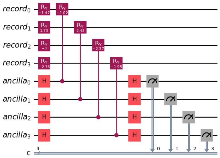
We use angle encoding because we previously discussed its advantages. However, we do not use its dense version because of clarity and easier implementation. In this simple version, we only use RY rotation. Here, we are not using QFT for addition or subtraction, so it is acceptable. We do this in lines 7 and 8 of Algorithm 5. Lines 11–14 present the steps of the Hadamard test. The CRY gate is used because the unitary Q in the Hadamard test must be applied conditioned on the first qubit or ancilla. The ancilla is the controlling qubit, and ${\psi }_r$ is the target qubit. The same $\theta$ is used for the Hadamard test and angle encoding. This reduces the computational overhead while encoding information about the relationship between the record and centroid in ${\psi }_r$. We did not encode the centroid into a quantum state; instead, we encode it in the rotation gate parameter $\theta$. Everything we want to know about it is in $\theta$. Finally, we measure the ancilla and use the probability that it is zero to calculate the sum of the phases of the record and the centroid. Since we apply the Hadamard test for each dimension separately, we add the probabilities to obtain the general likelihood. We demonstrate the rationale for setting the ancilla probability to zero and the relationship between this and the dissimilarity measure using equations later. The circuit diagram for Algorithm 5 is illustrated in Figure 1.

Algorithm 5 Rotational-Difference Quantum Heuristic Dissimilarity Measure

Require: Classical vectors $\mathbf{r},\mathbf{c}\in {\mathbb{R}}^n$, Number of shots S Ensure: Estimated quantum dissimilarity score D between $\mathbf{r}$ and $\mathbf{c}$   1: $n\leftarrow \left|\mathbf{r}\right|$                                                                   // Dimensionality of input vectors   2: Initialize quantum registers: $R_r\left[n\right]$, $R_a\left[n\right]$                                      // Record, ancilla   3: Initialize classical register: $C\left[n\right]$   4: ${\mathit{\theta }}_r\leftarrow {[2arcsin\left(r_i\right)]}_{i=0}^{n-1}$                                               // Compute rotation angles for $\mathbf{r}$   5: ${\mathit{\theta }}_c\leftarrow {[2arcsin\left(c_i\right)]}_{i=0}^{n-1}$                                               // Compute rotation angles for $\mathbf{c}$   6: Prepare quantum circuit Q with $R_r$, $R_a$, C   7: for $i=0$ to $n-1$ do   8:       $Q.RY({\theta }_{r,i},R_r\left[i\right])$                                                                            // Encode $\mathbf{r}$ into $R_r$   9: end for 10: $\theta ={\displaystyle \frac{{\theta }_c-{\theta }_r}{2}}$ 11: for $i=0$ to $n-1$ do 12:       $Q.H\left(R_a\left[i\right]\right)$                                                                  // Apply Hadamard to ancilla 13:       $Q.CRY(\theta ,R_a\left[i\right],R_r\left[i\right])$                                                            // Controlled rotation 14:       $Q.H\left(R_a\left[i\right]\right)$                                                                  // Apply Hadamard to ancilla 15: end for 16: $Q.\mathrm{Measure}(R_a,C)$                                                                // Measure ancilla register 17: $\mathrm{counts}\leftarrow \mathrm{Execute}(Q,S)$                                                                 // Run circuit S times 18: $P_0\leftarrow 0$ 19: for each $\mathrm{bitstring}b$ in counts do 20:       $P_0\leftarrow P_0+\left({\displaystyle \frac{\mathrm{Number}\mathrm{of}0\mathrm{s}\mathrm{in}b}{n}}\right)·\left({\displaystyle \frac{\mathrm{counts}\left[b\right]}{S}}\right)$ 21: end for 22: ${\mathsf{\Phi }}_{acc}\leftarrow 2P_0-1$     // Estimated average rotational-difference similarity factor 23: $D\leftarrow \sqrt{2-2·{\mathsf{\Phi }}_{acc}}$                                           // Rotational-difference dissimilarity 24: return D

Below are the equations of our Algorithm, which prove its correctness:

1. Record State Encoding:

$$|{\psi }_{r,i}\rangle =RY\left({\theta }_{r,i}\right)|0\rangle =cos\left({\displaystyle \frac{{\theta }_{r,i}}{2}}\right)|0\rangle +sin\left({\displaystyle \frac{{\theta }_{r,i}}{2}}\right)|1\rangle$$

$$|{\psi }_r\rangle ={\displaystyle \underset{i=0}{\overset{n-1}{⨂}}}|{\psi }_{r,i}\rangle$$

2. Initial State:

$$|{\psi }_0{\rangle =|0\rangle }_{a_0}{|0\rangle }_{a_1}{\dots |0\rangle }_{a_{n-1}}\otimes |{\psi }_{r,0}{\rangle }_{r_0}|{\psi }_{r,1}{\rangle }_{r_1}\dots |{\psi }_{r,n-1}{\rangle }_{r_{n-1}}={\displaystyle \underset{i=0}{\overset{n-1}{⨂}}}{|0\rangle }_{a_i}\otimes {|{\psi }_{r,i}\rangle }_{r_i}$$

3. Step 1: First Hadamard on Ancilla:

$$|{\psi }_{1,i}{\rangle =H|0\rangle }_{a_i}\otimes |{\psi }_{r,i}{\rangle }_{r_i}={\displaystyle \frac{1}{\sqrt{2}}}\left({|0\rangle }_{a_i}+{|1\rangle }_{a_i}\right)\otimes {|{\psi }_{r,i}\rangle }_{r_i}$$

4. Controlled-RY Definition:

$$CRY\left({\theta }_i\right)=|0\rangle \langle 0|\otimes I+|1\rangle \langle 1|\otimes RY\left({\theta }_i\right)$$

$$RY\left({\theta }_i\right)=\left(\begin{array}{cc}cos\left({\displaystyle \frac{{\theta }_i}{2}}\right)& -sin\left({\displaystyle \frac{{\theta }_i}{2}}\right)\\ sin\left({\displaystyle \frac{{\theta }_i}{2}}\right)& cos\left({\displaystyle \frac{{\theta }_i}{2}}\right)\end{array}\right)$$

$$RY\left({\theta }_i\right)|{\psi }_{r,i}\rangle =cos\left({\displaystyle \frac{3{\theta }_{r,i}-{\theta }_{c,i}}{4}}\right)|0\rangle +sin\left({\displaystyle \frac{3{\theta }_{r,i}-{\theta }_{c,i}}{4}}\right)|1\rangle ,\mathrm{where}{\theta }_i={\displaystyle \frac{{\theta }_{r,i}-{\theta }_{c,i}}{2}}$$

5. Step 2: CRY on ${\psi }_r$:

$$|{\psi }_{2,i}\rangle ={\displaystyle \frac{1}{\sqrt{2}}}\left({|0\rangle }_{a_i}|{\psi }_{r,i}{\rangle }_{r_i}+{|1\rangle }_{a_i}RY\left({\displaystyle \frac{{\theta }_{r,i}-{\theta }_{c,i}}{2}}\right){|{\psi }_{r,i}\rangle }_{r_i}\right)$$

6. Step 3: Second Hadamard:

$$|{\psi }_{3,i}\rangle ={\displaystyle \frac{1}{2}}\left[{|0\rangle }_{a_i}\left(|{\psi }_{r,i}\rangle +RY\left({\displaystyle \frac{{\theta }_{r,i}-{\theta }_{c,i}}{2}}\right)|{\psi }_{r,i}\rangle \right)+{|1\rangle }_{a_i}\left(|{\psi }_{r,i}\rangle -RY\left({\displaystyle \frac{{\theta }_{r,i}-{\theta }_{c,i}}{2}}\right)|{\psi }_{r,i}\rangle \right)\right]$$

7. Measurement Probability:

$$P_i\left(0\right)={∥{\displaystyle \frac{1}{2}}\left(|{\psi }_{r,i}\rangle +RY\left({\displaystyle \frac{{\theta }_{r,i}-{\theta }_{c,i}}{2}}\right)|{\psi }_{r,i}\rangle \right)∥}^2={\displaystyle \frac{1}{2}}+{\displaystyle \frac{1}{2}}cos\left({\displaystyle \frac{{\theta }_{r,i}-{\theta }_{c,i}}{4}}\right)$$

8. Total Probability:

$$\mathrm{totalprob0}={\displaystyle \frac{1}{n}}{\displaystyle \sum _{i=0}^{n-1}}{P}_i\left(0\right)={\displaystyle \frac{1}{2}}+{\displaystyle \frac{1}{2n}}{\displaystyle \sum _{i=0}^{n-1}}cos\left({\displaystyle \frac{{\theta }_{r,i}-{\theta }_{c,i}}{4}}\right)$$

9. Average rotational-difference similarity factor:

$${\mathsf{\Phi }}_{acc}=\mathrm{Average}\mathrm{rotational-difference}\mathrm{similarity}\mathrm{factor}:=2·\mathrm{totalprob0}-1={\displaystyle \frac{1}{n}}{\displaystyle \sum _{i=0}^{n-1}}cos\left({\displaystyle \frac{{\theta }_{r,i}-{\theta }_{c,i}}{4}}\right)$$

10. Dissimilarity measure

$$\mathrm{dissimilarity}\mathrm{score}=\sqrt{2-2·{\mathsf{\Phi }}_{acc}}$$

Our quantum-k-means using the Hadamard test (QK-H) is identical to its classical counterpart, except that we use Algorithm 5 to compute the dissimilarity score and use that for cluster assignment rather than Euclidean distances. The centroid update step follows the classical arithmetic mean, which is not guaranteed to be the optimal minimizer under the proposed dissimilarity measure. Therefore, the overall algorithm should be understood as a heuristic, k-means-inspired procedure rather than an exact optimization of a well-defined objective.

4. Results

In this section, we evaluate the performance of our proposed quantum k-means algorithms.

4.1. Dataset Description:

To assess our algorithms, we consider six datasets of two groups. The synthetic dataset includes Blobs with 800 data points and four features, and Moon with 800 data points and a noise of 1.2. Real datasets include the Iris, Wine, Breast Cancer Wisconsin, and Noisy-Iris datasets. They are defined below:

• Blobs: Synthetic data set with isotropic Gaussian blobs, which is used for evaluating clustering algorithms.
• Moons: Synthetic data set containing two interleaved half-circles, often used to test nonlinear classifiers or clustering techniques.
• Iris: A real-world dataset of flower measurements from three iris species, commonly used for classification tasks.
• Wine: A dataset with chemical analysis of wines from three cultivars, used for classification and feature selection.
• Breast Cancer Wisconsin: A medical imaging–based dataset containing numerical features extracted from breast tissue biopsies. It is used for binary classification to distinguish malignant tumours from benign ones.

The Moon and Wisconsin breast cancer dataset has only two classes, so we chose k to be 2. For other datasets, we choose k to be 3. This is carried out using the elbow method. We use the PCA algorithm on the wine and Wisconsin breast cancer datasets, reducing them to four dimensions while retaining 99% of the original variance. The noisy Iris dataset is the original Iris data with Gaussian noise added, with a mean of 0 and a standard deviation of 0.5.

4.2. Evaluation Metrics

We use the evaluation metrics for unsupervised tasks, and especially clustering is introduced in [31,32,33,34,35,36,37]:

• Folkes and Mallows Coefficient (FMI): Measures similarity between clusters and ground truth by computing the geometric mean of precision and recall for pairs [36].
• Sum of Squared Errors (SSE): Quantifies cohesion as the sum of squared distances from each point to its cluster centroid, also known as SSW [36].
• Silhouette Coefficient (Sil): Combines cohesion and separation by measuring how similar an object is to its cluster compared to other clusters [36].
• Rand Index (RI): Measures the similarity between two partitions by computing the proportion of point pairs that are either clustered together or separately in both partitions [33].
• Adjusted Rand Index (ARI): Quantifies the similarity between two clusterings by correcting the Rand Index for chance agreement, resulting in a score that ranges from $-1$ (complete disagreement) to 1 (perfect agreement) [32].
• Normalized Mutual Information (NMI): Measures the statistical dependency between cluster assignments, normalized to account for differences in entropy, with values ranging from 0 (no mutual information) to 1 (perfect match) [34].
• Davies–Bouldin Index (DBI): Evaluates clustering quality based on intra-cluster compactness and inter-cluster separation; lower values indicate better-defined clusters [35].
• Homogeneity: A clustering satisfies homogeneity if all clusters contain only data points from a single class [31].
• Completeness: A clustering satisfies completeness if all the data points of a given class are assigned to the same cluster [31].

After applying the Hungarian algorithm to obtain an optimal one-to-one mapping between predicted cluster labels and ground-truth labels, we evaluate clustering performance using standard classification metrics. These metrics are computed on the aligned labels and complement traditional clustering evaluation measures such as NMI and ARI.

These values are aggregated over all classes to compute the final metrics.

• Accuracy: Accuracy measures the overall proportion of correctly classified instances [37]:

  $$\mathrm{Accuracy}={\displaystyle \frac{TP+TN}{TP+TN+FP+FN}}$$

  (1)
• Precision: Precision evaluates the correctness of positive predictions [37]:

  $$\mathrm{Precision}={\displaystyle \frac{TP}{TP+FP}}$$

  (2)
• Recall (Sensitivity): Recall measures the ability of the model to identify all relevant instances of a class [37]:

  $$\mathrm{Recall}={\displaystyle \frac{TP}{TP+FN}}$$

  (3)
• F1-Score The F1-score is the harmonic mean of precision and recall [37]:

  $$F1={\displaystyle \frac{2·(\mathrm{Precision}·\mathrm{Recall})}{\mathrm{Precision}+\mathrm{Recall}}}$$

  (4)

In these metrics, TP, TN, FP, and FN are defined in a one-vs-all manner for each class as follows [37]:

• True Positive (TP): The number of instances correctly assigned to a given class.
• False Positive (FP): The number of instances incorrectly assigned to a given class.
• False Negative (FN): The number of instances of a given class that are incorrectly assigned to other classes.
• True Negative (TN): The number of instances that do not belong to a given class and are also not assigned to that class.

We also use:

• N-ITE: The actual number of iterations k-means performs to converge.

4.3. Implementation Details

We run our code for these algorithms under the following conditions: thresh = $0.0001$, maxite =10, shots = 32 and 8192, optimizationlevel = 3.

• thresh: The stopping condition of the algorithm. Defined as the maximum difference between cluster centres in two consecutive iterations, measured by the Frobenius norm, at which the algorithm is considered to have converged.
• maxite: The maximum number of iterations the algorithm can perform.
• shots: The number of times the quantum circuit is executed.
• optimization-level: The level at which the simulator optimizes the quantum circuit.

The experiments performed were carried out using quantum simulators due to the limited availability of quantum devices. Noise models and multiple samplings were used to simulate real-world conditions. In addition to these, we also provide resource estimation results using a hardware-specific backend (FakeGuadalupeV2) after transpiling to give a more realistic view of hardware limitations, e.g., qubit connectivity, native gate set restrictions.

We implemented our quantum circuits using Qiskit, an open-source quantum computing framework, and executed them using the AerSimulator (version 0.17.1). [38]. The AerSimulator, part of Qiskit’s Aer module, supports high-performance simulation of quantum circuits with up to 32 qubits by default (extendable with configuration), offering features like state vector, density matrix, and stabilizer simulations, as well as noise modeling for realistic quantum device emulation.

We consider two classical baselines for comparison: (1) standard classical k-means using Euclidean distance, and (2) a modified classical k-means (denoted as K-N) that uses the same dissimilarity measure introduced in our second method, computed classically using Equations (9) and (10). This allows for a fair comparison by isolating the effect of the proposed dissimilarity measure from the quantum estimation procedure. To ensure full reproducibility of the experiments, we fixed random seeds at three levels: (i) numpy.random.seed(42) and random.seed(42) for any classical randomness (e.g., centroid initialization and synthetic datasets), (ii) seed_simulator = 42 for Qiskit’s AerSimulator to obtain deterministic measurement outcomes, and (iii) seed_transpiler = 42 in the transpile() call to make the circuit-routing and optimization process repeatable. We have used the linear_sum_assignment function from scipy. optimize library for implementing the Hungarian algorithm to find the optimal one-to-one mapping between clusters and ground-truth labels by maximizing the total number of correctly assigned points across all K clusters.

To evaluate performance under realistic NISQ-like conditions, we incorporated a custom noise model in our simulator.

Depolarizing Gate Noise: Gate imperfections were modeled using depolarizing errors. Single-qubit gates (rz, sx, x, h, ry) were assigned an error rate of $p_{1q}=0.0005,$ while two-qubit entangling gates (cx) were assigned a higher error rate of $p_{2q}=0.005,$ reflecting the dominant contribution of entangling operations to noise in practical devices.

Thermal Relaxation Noise: Decoherence was modeled via thermal relaxation channels using coherence times $T_1=200\mathsf{\mu }\mathrm{s},T_2=160\mathsf{\mu }\mathrm{s}$. Thermal relaxation noise was implemented using the built-in thermal_relaxation_error function from Qiskit Aer. The resulting noise channel is represented using the Kraus operator formalism and applied according to the specified gate durations. Gate durations were set to $t_{1q}=45\mathrm{ns},$ $t_{2q}=220\mathrm{ns}$. These values provide relatively long coherence compared to gate execution time, resulting in a weaker relaxation effect.

Readout Noise: Measurement imperfections were modeled using a symmetric bit-flip readout error with probability: $p_{\mathrm{flip}}=0.008.$

All simulations were carried out on a density matrix simulation backend that allows us to account for noise from both coherent and incoherent sources.

Here we use $f=2$. For k-means clustering, it is not necessary to have the actual distances between data points but rather their relative values; therefore, this selection of f is a compromise between accuracy and circuit depth. If, however, we choose $f=1$, this results in too much discretization that will negatively impact the clustering process. Higher values of f lead to better numerical value representation but increase circuit depth and computing costs.

Before model training or clustering—specifically, before feeding data into our models—it is crucial to apply preprocessing to ensure uniformity and enhance performance. Two popular preprocessing techniques are:

• Standardization: Adjusts each feature so that it has a mean of zero and a standard deviation of one.
• Normalization: Rescales values either into a fixed range or such that each vector has a unit length. Of all the normalization techniques to be used, the ${\ell }_1$ and ${\ell }_{\infty }$ norms are evaluated. In this case, the ${\ell }_{\infty }$-norm technique is chosen, where the data is scaled according to the maximum absolute values in each observation. This is performed because ${\ell }_{\infty }$ normalization works effectively within the framework of this particular encoding mechanism, as it ensures that all values are within a specified range suitable for rotation-based encoding.

This preprocessing is performed on the whole dataset rather than just part of it. And first we have Standardization, then Normalization.

The final results are averaged over 10 runs with different random initializations (k-means++), along with the corresponding standard deviations.

The implementation of the proposed method is publicly available at https://github.com/shahin-torabii/Quantum-k-means-Clustering-Using-Phase-Accumulation-via-Hadamard-Test (accessed on 27 May 2026).

4.4. Evaluation

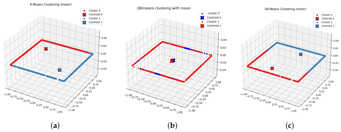
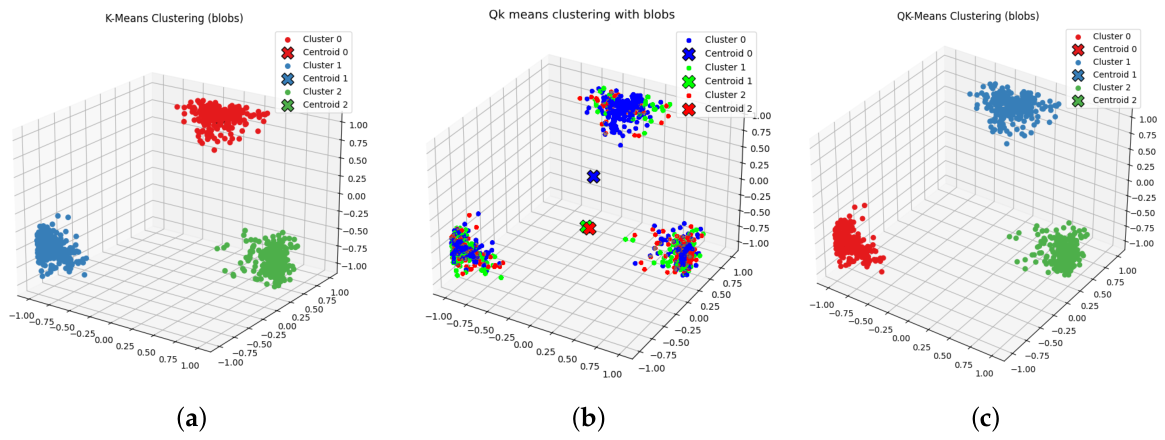
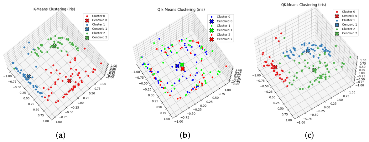
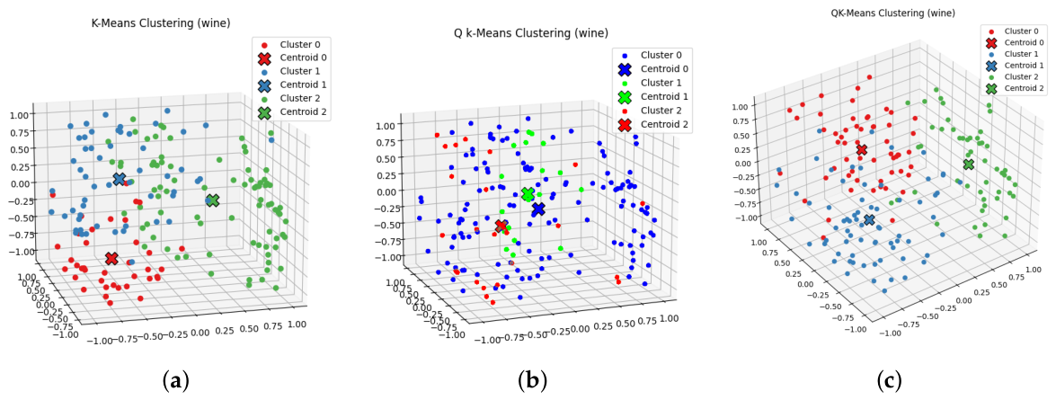
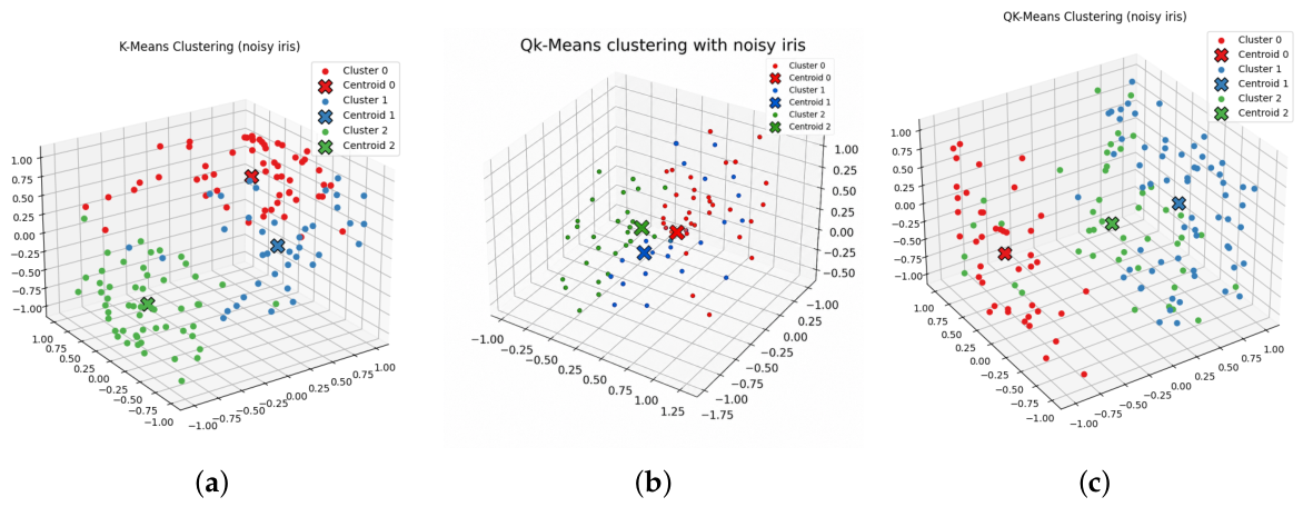
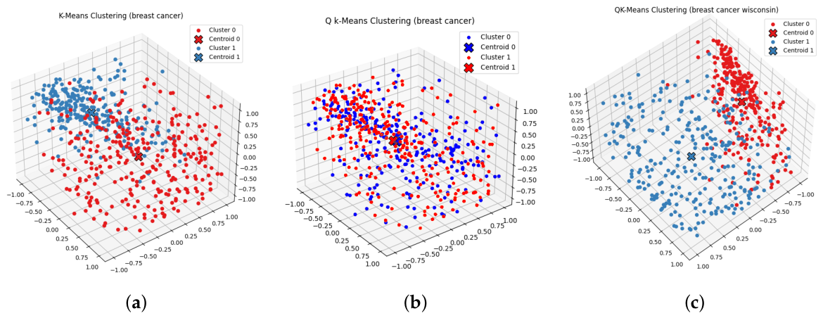
Results of classical k-means, classical k-means using the new metric(K-N), quantum k-means using the Hadamard test with 8192 shots(QK-H) and 32 shots (QK-H-32), quantum k-means using QFT-based addition(QK-QFT), and the quantum approach introduced in [8] are shown in

Table 3. Clustering comparison (Part I: internal clustering metrics).

Dataset	N-ITE	SSE	SIL	DBI	ARI	NMI
IRIS
IRIS-K	5.0 ± 0.0000	61.6802 ± 0.0000	0.5312 ± 0.0000	0.7619 ± 0.0000	0.6038 ± 0.0000	0.6552 ± 0.0000
IRIS-K-N	6.8 ± 2.7856	326.4160 ± 265.5407	0.4566 ± 0.2102	1.0354 ± 0.4786	0.4807 ± 0.3326	0.4962 ± 0.3318
IRIS-QK-H	4.7 ± 1.4178	63.226 ± 0.0000	0.527 ± 0.0000	0.743 ± 0.0000	0.609 ± 0.0000	0.650 ± 0.0000
IRIS-QK-H-32	5.2 ± 1.4697	63.6309 ± 0.8542	0.5244 ± 0.0092	0.7526 ± 0.0381	0.5959 ± 0.0227	0.6413 ± 0.0238
IRIS-QK-QFT	10	307.2400	0.041	19.0300	0.0070	0.0070
IRIS-QK-R [8]	7	616.830	0.4800	–	–	–
WINE
WINE-K	5.0 ± 0.0000	206.8692 ± 0.0000	0.2039 ± 0.0000	1.5049 ± 0.0000	0.3093 ± 0.0000	0.3199 ± 0.0000
WINE-K-N	7.0 ± 3.0822	392.2134 ± 257.8630	0.4390 ± 0.2316	1.1085 ± 0.5094	0.4487 ± 0.3649	0.4577 ± 0.3608
WINE-QK-H	6.6 ± 2.5377	184.6930 ± 5.9280	0.2830 ± 0.0210	1.399 ± 0.0820	0.6090 ± 0.1200	0.5760 ± 0.0940
WINE-QK-H-32	8.8 ± 1.9890	189.6016 ± 10.6955	0.2670 ± 0.0352	1.4251 ± 0.1264	0.5534 ± 0.1600	0.5422 ± 0.1430
WINE-QK-QFT	10	310.370	0.0200	16.4000	0.0060	0.0050
BLOBS
BLOBS-K	2.0 ± 0.0000	75.5599 ± 0.0000	0.8277 ± 0.0000	0.2515 ± 0.0000	1.0000 ± 0.0000	1.0000 ± 0.0000
BLOBS-K-N	5.5 ± 3.5000	365.0366 ± 289.4766	0.5705 ± 0.2572	0.8140 ± 0.5625	0.7504 ± 0.2496	0.7491 ± 0.2509
BLOBS-QK-H	1.1 ± 0.3000	75.560 ± 0.0000	0.828 ± 0.0000	0.252 ± 0.0000	1.000 ± 0.0000	1.000 ± 0.0000
BLOBS-QK-H-32	1.1 ± 0.3000	75.5599 ± 0	0.8277 ± 0	0.2515 ± 0	1.0000 ± 0	1.0000 ± 0
BLOBS-QK-QFT	10	1546.4400	0.0030	20.4900	0.0670	0.0580
BLOBS-QK-R [8]	7	422.2300	0.8600	–	–	–
MOON
MOON-K	7.0 ± 0.0000	581.3156 ± 0.0000	0.4288 ± 0.0000	1.0842 ± 0.0000	0.1267 ± 0.0000	0.0943 ± 0.0000
MOON-K-N	7.0 ± 3.5590	455.9653 ± 269.0735	0.5097 ± 0.2269	0.9535 ± 0.4998	0.4999 ± 0.4087	0.4994 ± 0.4082
MOON-QK-H	5.3 ± 2.4515	590.9730 ± 20.3440	0.4210 ± 0.0160	1.1100 ± 0.0520	0.1010 ± 0.0480	0.0750 ± 0.0350
MOON-QK-H-32	5.6 ± 2.6533	592.4755 ± 22.7411	0.4205 ± 0.0171	1.1122 ± 0.0560	0.0989 ± 0.0486	0.0737 ± 0.0358
MOON-QK-QFT	10	987.2000	0.0030	20.1600	0.0010	0.0010
MOON-QK-R [8]	5	7185.8000	0.5500	–	–	–
NOISY IRIS
NOISY-IRIS-K	8.0 ± 0.0000	108.0471 ± 0.0000	0.3864 ± 0.0000	1.0494 ± 0.0000	0.5294 ± 0.0000	0.5505 ± 0.0000
NOISY-IRIS-K-N	6.84 ± 2.5440	291.4000 ± 254.7363	0.4401 ± 0.1954	1.0352 ± 0.4369	0.4796 ± 0.3036	0.4959 ± 0.3029
NOISY-IRIS-QK-H	6.9 ± 2.6627	114.2470 ± 1.5310	0.3440 ± 0.0090	1.1010 ± 0.0300	0.4540 ± 0.0460	0.5230 ± 0.0380
NOISY-IRIS-QK-H-32	7.7 ± 2.4515	122.3730 ± 9.6597	0.3144 ± 0.0330	1.1983 ± 0.1568	0.3728 ± 0.0961	0.4269 ± 0.1044
NOISY-IRIS-QK-QFT	10	280.2360	0.0230	0.0100	0.0120	0.0100
BCW
BCW-K	10.0 ± 0.0000	649.5961 ± 0.0000	0.3191 ± 0.0000	1.3455 ± 0.0000	0.4521 ± 0.0000	0.4667 ± 0.0000
BCW-K-N	9.0 ± 0.0000	654.5132 ± 0.0000	0.3133 ± 0.0000	1.3765 ± 0.0000	0.5008 ± 0.0000	0.4981 ± 0.0000
BCW-QK-H	8.6 ± 1.6852	662.9880 ± 20.5510	0.3060 ± 0.0180	1.4110 ± 0.0850	0.4470 ± 0.1380	0.4390 ± 0.1400
BCW-QK-H-32	9.3000 ± 1.4177	674.4183 ± 33.7576	0.2961 ± 0.0308	1.4572 ± 0.1558	0.4245 ± 0.1706	0.4044 ± 0.1732
BCW-QK-QFT	10	961.9470	0.0000001	24.2740	0.0001	0.0000002

and

Table 4. Clustering comparison (Part II: external and classification metrics).

Dataset	HOM	FMI	COMP	Precision	Accuracy	Recall	F1-Score
IRIS
IRIS-K	0.6503 ± 0.0000	0.7363 ± 0.0000	0.6601 ± 0.0000	0.8278 ± 0.0000	0.8200 ± 0.0000	0.8200 ± 0.0000	0.8178 ± 0.0000
IRIS-K-N	0.4968 ± 0.3312	0.7066 ± 0.1804	0.4957 ± 0.3326	0.7745 ± 0.1799	0.7571 ± 0.1799	0.7571 ± 0.1799	0.7572 ± 0.1797
IRIS-QK-H	0.6420 ± 0.0000	0.7410 ± 0.0000	0.6590 ± 0.0000	0.8420 ± 0.0000	0.8270 ± 0.0000	0.8270 ± 0.0000	0.8230 ± 0.0000
IRIS-QK-H-32	0.6334 ± 0.0191	0.7324 ± 0.0174	0.6494 ± 0.0287	0.8327 ± 0.0211	0.8180 ± 0.0133	0.8180 ± 0.0133	0.8150 ± 0.0111
IRIS-QK-QFT	0.0770	0.3500	0.0080	0.3790	0.3730	0.3730	0.3590
IRIS-QK-R [8]	–	–	–	–	–	–	–
WINE
WINE-K	0.3152 ± 0.0000	0.5503 ± 0.0000	0.3247 ± 0.0000	0.5659 ± 0.0000	0.5787 ± 0.0000	0.5787 ± 0.0000	0.5603 ± 0.0000
WINE-K-N	0.4606 ± 0.3613	0.6979 ± 0.2007	0.4549 ± 0.3605	0.7577 ± 0.1976	0.7398 ± 0.1973	0.7398 ± 0.1973	0.7407 ± 0.1974
WINE-QK-H	0.5760 ± 0.0940	0.7410 ± 0.0790	0.5760 ± 0.0950	0.8520 ± 0.0760	0.8390 ± 0.0840	0.8390 ± 0.0840	0.8410 ± 0.0840
WINE-QK-H-32	0.5405 ± 0.1441	0.7064 ± 0.1031	0.5440 ± 0.1418	0.8325 ± 0.0859	0.8140 ± 0.0953	0.8140 ± 0.0953	0.8149 ± 0.0957
WINE-QK-QFT	0.0050	0.3330	0.0050	0.3780	0.3640	0.3640	0.3650
BLOBS
BLOBS-K	1.0000 ± 0.0000	1.0000 ± 0.0000	1.0000 ± 0.0000	1.0000 ± 0.0000	1.0000 ± 0.0000	1.0000 ± 0.0000	1.0000 ± 0.0000
BLOBS-K-N	0.7552 ± 0.2448	0.8791 ± 0.1209	0.7432 ± 0.2568	0.9459 ± 0.0541	0.9271 ± 0.0729	0.9271 ± 0.0729	0.9283 ± 0.0717
BLOBS-QK-H	1.0000 ± 0.0000	1.0000 ± 0.0000	1.0000 ± 0.0000	1.0000 ± 0.0000	1.0000 ± 0.0000	1.0000 ± 0.0000	1.0000 ± 0.0000
BLOBS-QK-H-32	1.0000 ± 0.0000	1.0000 ± 0.0000	1.0000 ± 0.0000	1.0000 ± 0.0000	1.0000 ± 0.0000	1.0000 ± 0.0000	1.0000 ± 0.0000
BLOBS-QK-QFT	0.0570	0.3870	0.0590	0.4650	0.4530	0.4650	0.4550
BLOBS-QK-R [8]	–	–	–	0.9980	0.9980	0.9980	0.9980
MOON
MOON-K	0.0943 ± 0.0000	0.5628 ± 0.0000	0.0943 ± 0.0000	0.6788 ± 0.0000	0.6788 ± 0.0000	0.6788 ± 0.0000	0.6787 ± 0.0000
MOON-K-N	0.5035 ± 0.4083	0.7524 ± 0.2047	0.4955 ± 0.4083	0.7985 ± 0.2131	0.7860 ± 0.2082	0.7860 ± 0.2082	0.7868 ± 0.2085
MOON-QK-H	0.0750 ± 0.0350	0.5500 ± 0.0240	0.0750 ± 0.0350	0.6500 ± 0.0550	0.6500 ± 0.0550	0.6500 ± 0.0550	0.6500 ± 0.0550
MOON-QK-H-32	0.0737 ± 0.0358	0.5491 ± 0.0239	0.0737 ± 0.0358	0.6465 ± 0.0595	0.6465 ± 0.0595	0.6465 ± 0.0595	0.6464 ± 0.0597
MOON-QK-QFT	0.0010	0.5000	0.0010	0.5130	0.5130	0.5130	0.5120
MOON-QK-R [8]	–	–	–	0.9800	0.9800	0.9800	0.9800
NOISY IRIS
NOISY-IRIS-K	0.5455 ± 0.0000	0.6873 ± 0.0000	0.5557 ± 0.0000	0.7814 ± 0.0000	0.7800 ± 0.0000	0.7800 ± 0.0000	0.7734 ± 0.0000
NOISY-IRIS-K-N	0.4951 ± 0.3023	0.6976 ± 0.1659	0.4968 ± 0.3036	0.7684 ± 0.1648	0.7543 ± 0.1643	0.7543 ± 0.1643	0.7522 ± 0.1644
NOISY-IRIS-QK-H	0.5200 ± 0.0390	0.6350 ± 0.0300	0.5250 ± 0.0360	0.7020 ± 0.0470	0.6930 ± 0.0520	0.6930 ± 0.0520	0.6950 ± 0.0510
NOISY-IRIS-QK-H-32	0.4140 ± 0.1778	0.7225 ± 0.0808	0.3951 ± 0.1689	0.8446 ± 0.0936	0.8146 ± 0.0864	0.8146 ± 0.0864	0.8172 ± 0.0856
NOISY-IRIS-QK-QFT	0.0120	0.0120	0.0120	0.3340	0.3790	0.3790	0.3790
BCW
BCW-K	0.4777 ± 0.0000	0.7350 ± 0.0000	0.4562 ± 0.0000	0.8827 ± 0.0000	0.8366 ± 0.0000	0.8366 ± 0.0000	0.8391± 0.0000
BCW-K-N	0.5104 ± 0.0000	0.7583 ± 0.0000	0.4864 ± 0.0000	0.8918 ± 0.0000	0.8541 ± 0.0000	0.8541 ± 0.0000	0.8565 ± 0.0000
BCW-QK-H	0.4500 ± 0.1430	0.7320 ± 0.0670	0.4290 ± 0.1370	0.8620 ± 0.0800	0.8260 ± 0.0770	0.8260 ± 0.0770	0.8290 ± 0.0760
BCW-QK-H-32	0.3520 ± 0.1700	0.8100 ± 0.1000	0.3400 ± 0.1600	0.8140 ± 0.1100	0.8080 ± 0.1000	0.8080 ± 0.1000	0.8110 ± 0.1000
BCW-QK-QFT	0.0000003	0.3330	0.000001	0.5330	0.5040	0.5040	0.5130

. Table 3 shows internal clustering metrics, and Table 4 shows external and classification metrics. The results of these three methods are shown in Figure 2, Figure 3, Figure 4, Figure 5, Figure 6 and Figure 7.

The comparison between classical k-means (K) and the quantum variant based on the Hadamard test (QK-H) shows that QK-H is able to match closely, and in some cases surpass, the performance of its classical counterpart. On well-structured datasets such as IRIS and BLOBS, the two methods exhibit nearly identical behavior in terms of cluster compactness (as reflected by SSE), cluster separation (silhouette score and DBI), and class alignment (ARI and accuracy). For instance, the SSE for QK-H and K is 63.23 and 61.68, respectively, on the IRIS dataset. ARI and accuracy for QK-H clusterings were obtained at 0.609 and 0.827 levels, respectively, whereas for K clusterings, 0.6038 and 0.820. This demonstrates that there is a similar compactness level and marginally better alignment to ground truth labels. In addition, in the case of BLOBS data, both clustering techniques achieve perfect scores (e.g., ARI = 1.0, accuracy = 1.0). Importantly, for WINE data, there is a significantly better performance of QK-H compared to K, based on the smaller SSE value (184.69 compared to 206.87), better separation (with increased silhouette score from 0.2039 to 0.283, and reduction in DBI), and improved matching with the true classes (increase in ARI from 0.3093 to 0.609, and increase in accuracy from 0.5787 to 0.839). These results suggest that the Hadamard-test-based dissimilarity can capture different structural relationships in higher-dimensional feature spaces compared to Euclidean distance.

Nevertheless, this trend does not apply to all types of datasets. In more difficult cases where noise and nonlinear structures are present, QK-H is expected to demonstrate a slight inferiority compared to K-Means concerning the criteria mentioned above. Specifically, the NOISY IRIS data set indicates that the algorithm performs poorly compared to its predecessor when assessing the quality of clustering using such measures as SSE, silhouette score, and ARI (114.25 vs. 108.05, 0.344 vs. 0.3864, 0.454 vs. 0.5294, respectively). Similar results were obtained with the MOON data set, which poses an additional challenge to both methods due to its nonlinearity; however, QK-H yields slightly lower performance than K-Means on certain metrics (ARI, for example, 0.101 vs. 0.1267; accuracy: 0.650 vs. 0.6788). The BCW data set demonstrates almost identical performance of both algorithms, with minor losses for QK-H (accuracy: 0.826 vs. 0.8366). This disparity may partially result from the fact that the QK-H algorithm relies on probabilistic estimates of similarity and is therefore sensitive to noise. Overall, QK-H represents a competitive and even better alternative in many cases of structured and multidimensional data, yet further improvements are possible.

The comparison between classical K-Means (K) and its modified variant using the Hadamard-test-inspired dissimilarity (K-N) shows that replacing Euclidean distance with a non-Euclidean metric introduces a trade-off between cluster structure quality and class alignment. As far as internal cluster properties are concerned, K-N generally leads to worse cluster compactness and separation based on the IRIS and BLOBS data sets (IRIS: SSE 326.42 vs. 61.68; SIL 0.4566 vs. 0.5312; BLOBS: SSE 365.04 vs. 75.56; SIL 0.5705 vs. 0.8277). The findings show that clusters have worse cohesion and coherence when calculated using the proposed metric. In regard to the external evaluation metrics, on the other hand, K-N can improve agreement with the ground truth classification on several cases, especially in those cases where the data set is more complicated, such as WINE (ARI 0.4487 vs. 0.3093; Accuracy 0.7398 vs. 0.5787) and MOON (ARI 0.4999 vs. 0.1267), which suggests that the new metric includes label-related structure while Euclidean distance may not. In general, it seems that K is better at creating coherent clusters, while K-N tends to create clusters that better agree with the label structure. In particular, K dominates on internal metrics across IRIS and BLOBS, whereas K-N is stronger on external metrics for WINE and MOON.

The comparison between K-N and QK-H shows that introducing a probabilistic quantum estimation of the same non-Euclidean dissimilarity generally leads to more consistent clustering behavior. In terms of internal structure, K-N often produces weaker compactness and separation. On the other hand, QK-H tends to improve or restore the quality of clustering, as seen in IRIS (SSE: 63.23 vs. 326.42, SIL: 0.527 vs. 0.4566) and WINE (SSE: 184.69 vs. 392.21, SIL: 0.283 vs. 0.4390), and achieves near-optimal performance on BLOBS. However, this improvement is not universal. K-N can still achieve competitive or even better class alignment in certain cases, such as MOON (ARI: 0.4999 vs. 0.101, accuracy: 0.786 vs. 650) or NOISY IRIS (accuracy: 0.754 vs. 0.693) and Breast Cancer (ARI: 0.500 vs. 0.447), indicating that it may better capture label structure in noisy or complex datasets. Generally, it can be said that QK-H is able to behave much better and more reliably on the considered datasets, resulting in better structural clustering quality without deteriorating its external performance. Thus, it seems that the process of quantum estimation plays some role in achieving better clustering quality.

The results suggest that the observed improvements in QK-H over K-Means cannot be attributed solely to the replacement of the similarity metric, since K-N—despite using the same dissimilarity in a fully classical setting—does not consistently outperform classical K-Means and often shows only limited or unstable gains. It means that the operation of K-N could be influenced by the inconsistency of the non-Euclidean dissimilarity with the procedure of centroids updating, limiting the degree to which the dissimilarity helps to reveal the cluster structure. In turn, QK-H outperforms K-N on several occasions (for instance, for IRIS and WINE data sets in terms of both external and internal metrics) and even classical K-Means in some cases, indicating that QK-H’s performance does not depend entirely on the choice of similarity measure. Instead, the behavior of QK-H—particularly its lower SSE values and observed variability—may be partly influenced by its stochastic, measurement-based estimation process. In one such interpretation, the stochastic nature could itself serve as a perturbation mechanism, facilitating the exploration of alternate partition possibilities by QK-H and allowing it to sidestep some non-ideal local optimum solutions at times. Yet this feature is by no means constant for every data set, and may be one factor behind the varying effectiveness of QK-H under different conditions. Thus, the operation of QK-H is best explained by the dual impact of its modified dissimilarity measure and its stochastic estimation procedure.

The number of shots is an important practical consideration for the implementation of algorithms in quantum computation due to the inherent probabilistic measurement process involved. An increase in the number of shots generally leads to improved accuracy in estimating the similarity metric, as seen in Table 3 and Table 4, where results obtained with 8192 shots are more stable. However, increasing the number of shots also significantly increases computational cost. A comparison of QK-H with a large number of shots (8192) with its low shot counterpart QK-H-32 reveals that a considerable savings on the measurement budget has little impact on clustering accuracy. For most of the data sets considered, the two algorithms are close to each other in both internal and external criteria measures. As an instance, on the IRIS data set, both the techniques show almost equal results (SSE: 63.63 against 63.23; SIL: 0.5244 against 0.527). Likewise, on the WINE data set, QK-H-32 demonstrates almost similar clustering tendencies (SSE: 189.60 vs. 184.69, SIL: 0.2670 vs. 0.283, ARI: 0.5534 vs. 0.609). In fact, the performance does not change much even on the more complicated datasets, such as MOON and NOISY IRIS, where it shows moderate differences (ARI MOON = 0.0989 vs. 0.101; ARI NOISY IRIS = 0.3728 vs. 0.454). Therefore, the lower-shot version follows the same clustering tendency even with higher stochastic variations. In general, we can conclude that the data prove that the 32-shot model sufficiently approximates the model using 8192 shots, following a similar clustering trend but consuming significantly less computational power. Thus, the results show that the quality of quantum clustering is not very sensitive to the number of shots used for sampling. The approach works well when using fewer samples, which makes it more applicable for immediate deployment. However, more shots are mainly used to measure estimation precision.

When comparing error bars for the three cases of K-Means (K), QK-H (8192 shots), and QK-H-32, there exist clear distinctions in terms of stability and repeatability. The classical K-Means approach usually has very little variance between multiple runs, for example, in IRIS distance measurements (±0.000). In turn, the QK-H shows a reasonable variability owing to its probabilistic-based estimation process, where the obtained standard deviations are relatively low but still existent for each metric, as is the case with ARI fluctuations on WINE and NOISY IRIS. The same is true for QK-H-32, which shows similar variability but with slightly exaggerated variability in some cases; however, it stays consistently close to its full-shot counterpart in terms of average results. Importantly, the variance of both quantum setups is limited and consistent among different datasets, which suggests that the probabilistic approximation algorithm does not lead to unstable cluster formation. All in all, K-Means turns out to be a deterministic algorithm, whereas QK-H and QK-H-32 are stable algorithms with consistent performance based on aggregate indicators. It can be concluded that despite the presence of randomness introduced by quantum measurement, the structure of clusters is maintained even with significantly smaller shot costs.

From comparing the rate of convergence, it can be seen that QK-H always requires a similar or slightly lesser number of iterations compared to the traditional K-Means algorithm, while K-N lacks consistency. As an example, the IRIS data set has an average convergence of 4.7 iterations using QK-H, 5.0 with K, and 6.8 with K-N. On BLOBS, QK-H converges notably faster (1.1 vs. 2.0). Similar trends are observed on other datasets, although the improvement is not uniform. In contrast, K-N does not show consistent convergence behavior: it converges faster than K-Means in some cases, such as NOISY IRIS (6.84 vs. 8.0) and BCW (9.0 vs. 10.0), but slower in others, including IRIS and WINE. On the other hand, the QK-H-32 low shot variant shares similar convergence behavior with QK-H, albeit with slight differences (for instance, IRIS = 5.2, BLOBS = 1.1, MOON = 5.6). The implication is that decreasing the shots will not make much difference in terms of convergence behavior. Taken together, QK-H and QK-H-32 converge faster than classical K-Means, with some cases even surpassing K-N.

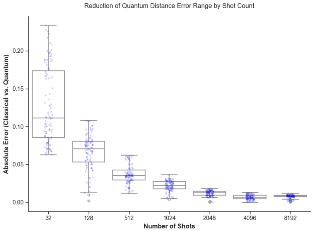
Since K-N represents the analytical form of the QK-H dissimilarity measure, the quantum estimation is expected to approach the classical value as the number of shots increases. To validate this behavior, we performed a pointwise comparison using 100 random vector pairs under an idealized (noiseless) simulation. As shown by the box plot presented in Figure 8, there is a significant variation in the absolute error with $N=32$ shots (0.05–0.20), which is characteristic of stochastic sampling error. However, as N increases, the distribution of errors decreases significantly, such that when $N\ge 512$, the error drops below 0.05. It is important to note that this convergence is observed under ideal conditions. In a realistic noisy environment, as used for the results in Table 3 and Table 4, a baseline error (typically >0.1) persists even at high shot counts. Higher shot numbers are used in order to minimize sampling errors, but systematic error terms cannot be minimized since there are still gate infidelities and decoherence issues. This explains why there is a disparity between the outcomes of K-N versus QK-H.

The depth-optimized circuit of the proposed QK-H approach has a depth of approximately 4 before transpilation, which is relatively shallow for Hadamard-test-based constructions. Upon compilation to the hardware-aware backend (FakeGuadalupeV2), there is an observable similarity in the circuits’ structure regardless of the data set. They have a consistent architecture with a total of 16 qubits and circuit depth of 10 (12 for the MOON dataset). The number of two-qubit gates (CX) is minimal, ranging from 3 to 8, whereas the one-qubit gate (RZ) is roughly 16 to 34, and SX is from 10 to 16. Based on the results obtained, the designs are expected to have shallow circuit depth after transpilation and involve few entangling gates. These two key factors cause noise in current quantum computers. Therefore, it is plausible that the technique can fit in with the limitations of near-term quantum hardware. In particular, the low CX count and moderate circuit depth are in line with, or lower than, those reported for several quantum distance estimation approaches that require deeper circuits or more entangling layers. In addition, the method is based on a simple architecture employing the Hadamard test along with rotation encoding, without resorting to any complex subroutines like amplitude estimation or complex interference circuits. Along with the demonstrated robustness under a lower number of repetitions (32 repetitions), the above findings indicate that the method would be viable even under resource-constrained conditions. However, it must be acknowledged that the experimental results presented above have been obtained through simulation on a virtual backend, and other noise effects associated with physical quantum computing systems could affect its performance.

The time complexity of the proposed distance evaluation is $O\left(MKSn\right)$. Here, n is the number of features, K is the number of centroids, S is nd the number of measurement shots. For a single record–centroid comparison, the quantum circuit applies feature-wise rotations followed by a Hadamard-test-based measurement, resulting in a circuit cost of $O\left(n\right)$ per execution. But since we need to perform S number of repetitions of each shot in order to obtain an exact estimate of probabilities, our comparison cost becomes $O\left(Sn\right)$. The assignment step in the k-means algorithm involves comparing M number of points to K number of centers. While features can be encoded using quantum circuits in parallel, each comparison between a point and the center requires separate execution and measurement of a quantum circuit. With the help of QRAM, it would have been possible to make the comparisons in superposition, bringing down per-iteration costs to $O\left(MSn\right)$. Since QRAM is not assumed in this theoretical work, comparisons are performed sequentially.

For the quantum QFT-based addition k-means (QK-QFT), comparing its results with both classical k-means and our QK-H method, as shown in Table 3 and Table 4, reveals that the QK-QFT approach performs significantly worse. Most clustering metrics—such as ARI, NMI, homogeneity, and completeness—are close to zero, indicating poor clustering quality. This is critical, as higher values generally represent better performance for most of these metrics (except SSE and DBI).

While the method shows relatively better performance on classification-based metrics (e.g., accuracy, precision, recall), these remain mediocre compared to the baseline methods. This suggests that although the QK-QFT correctly assigns some data points, the actual cluster structure is poorly defined, with significant overlaps between clusters.

Similarly, the circuit depth for QK-QFT is high as well. In particular, the depth of the circuit before transpilation is 60, resulting in poor performance within the NISQ era. This result is consistent with the earlier-mentioned circuit depth of $O(logn)$, but this applies to just one quantum adder based on QFT. In the case of the full quantum distance circuit, there are two quantum adders along with a quantum multiplication process implemented through Draper’s method. These additional components increase the overall circuit depth. Due to this depth, it is challenging to visualize its circuit properly. Its poor performance is due to its depth and, therefore, its proneness to noise.

Overall, the QFT-based k-means variant (QK-QFT) exhibits limited suitability for distance estimation in clustering tasks. In general, the technique demonstrates poor clustering accuracy in comparison with classic clustering methods and clustering based on the Hadamard test. These drawbacks are due to finite-precision coding, high circuit depth, and limited qubit resources. Though QFT-based computations provide a valid approach for calculating the Euclidean distance, the experimental results show that under real conditions, the technique is unable to perform accurate clustering. Thus, any conclusions based on the use of the QK-QFT must be considered in light of its drawbacks. Extra caution is needed while comparing QK-QFT. While classic k-means performs at almost an unlimited precision level, QK-QFT requires limited qubit numbers and finite-precision coding. The usage of increased precision for QK-QFT is unrealistic since it would require much larger qubits and greater circuit depth.

One possible limitation that has been identified in some of the existing research papers is the way the clustering ability of quantum clustering algorithms was assessed. Some researchers have used accuracy alone to evaluate the clustering ability, but no other clustering metrics were used. However, it is important to consider different clustering metrics since using accuracy alone does not help understand the various aspects of clustering. As can be seen from Table 3, we try to avoid this problem through our approach, thereby providing a more robust comparison between quantum and classical k-means.

It is also informative to compare our QK-H results with prior work to provide context for the performance of the proposed approach. Results from [8] are shown in Table 3 and Table 4. On the BLOBS dataset, our method achieves lower SSE, indicating improved compactness, while some other metrics are weaker. Performance-wise on IRIS, the difference lies in the fact that the number of iterations needed is greater in our method compared to [8]. In terms of MOON, however, we have achieved better results using our algorithm on SSE while underperforming on other alignment-based measures. Overall, the above comparisons show that both methods have different advantages since one performs better in terms of compactness while the other has better values for accuracy-oriented measures. It should be noted, however, that comparison was possible only because [8] did not provide all evaluation metrics (e.g., accuracy). In addition, the method in [8] relies on QRAM-based structures with higher circuit depth, whereas our approach uses a shallower circuit design. This suggests that our method may be more compatible with near-term hardware, although a fully controlled comparison would be required to confirm this. A comparison of the results from [19] and our method is presented in

Table 5. Accuracy on IRIS dataset with corresponding quantum circuit depth for different circuit designs with k = 2 (four designs from [19] and our two approaches).

Circuit	IRIS (K = 2)	Depth
Basic Implementation [19]	42.0	37
Optimized Interference [19]	62.0	25
Negative Rotations [19]	80.0	2
Distance Calc. (Destructive Interference) [19]	83.4	14
The Hadamard Test	75.7.0	10

. The only common dataset is IRIS, and the reported metrics in [19] are limited to accuracy and circuit depth. Among the implementations in [19], two achieve higher accuracy than our approach. In this regard, one particular technique, which makes use of the principle of destructive interference, stands out for its comparatively deep circuit structure compared to the one discussed here. However, other approaches, such as the one called Negative Rotations, offer comparable accuracy but are significantly less deep in their circuit structures. With the proposed QK-H circuit, whose post-transpilation depth is 10, similar results can be obtained while keeping the circuit depth relatively low. However, since clustering evaluation measures like ARI, NMI, and silhouette scores have not been reported in [19], an accurate evaluation cannot be provided. Overall, these results highlight differing trade-offs across methods in terms of accuracy, circuit depth, and evaluation scope. The datasets used in [7] differ from ours, and [6] does not report specific clustering accuracy results. Therefore, we exclude both from our evaluation.

In [22], only ARI results for the Iris dataset are reported, which we compare with our QK-H method in

Table 6. ARI values for quantum balanced k-means on Iris dataset variations.

(Points, Clusters)	ARI (Quantum Balanced k-Means) [22]	ARI (Quantum k-Means Using the Hadamard Test)
(8, 2)	0.76	1.0
(16, 2)	0.88	1.0
(24, 2)	0.91	1.0
(32, 2)	0.91	1.0
(9, 3)	0.72	0.31
(12, 3)	0.76	0.36
(15, 3)	0.77	0.64
(18, 3)	0.79	0.66
(21, 3)	0.71	0.6

. Although higher ARI values are reported in [22], their evaluation is performed on subsets of the Iris dataset, whereas in this work, the complete dataset of 150 records is also considered. The low ARI values of 0.31 and 0.36 for the $(9,3)$ and $(12,3)$ cases should be interpreted with caution. These results arise from the greater difficulty of the $k=3$ setting on very small randomly selected subsets, rather than indicating a general weakness of QK-H. In the Iris dataset, the three-class problem is inherently harder than the two-class case because versicolor and virginica classes overlap in feature space, whereas the $k=2$ subsets are comparatively easier. Moreover, small subsets are sensitive to random sampling and may not preserve the structure of the full dataset, which can lead to unstable ARI values. This is consistent with the improved ARI values for larger subsets and the stronger performance obtained on the complete dataset in Table 3.

Finally, the approach in [22] is implemented in an adiabatic quantum computing framework, which differs fundamentally from the gate-based model used in this work. In adiabatic approaches, computational complexity and implementation constraints are not characterized by circuit depth in the same manner as in gate-based quantum circuits, making direct performance comparison non-trivial. Moreover, the method in [22] uses balanced k-means, where the cluster sizes are constrained to be equal. This constraint may improve clustering performance under certain conditions, particularly when the sampled data approximately satisfy the balanced-cluster assumption. Therefore, differences in data volume, quantum computing model, and clustering criteria should be considered when comparing the two methods.

One notable work using the Breast Cancer Wisconsin dataset is [39]. A comparison of our results with theirs is provided in

Table 7. Comparison between our QK-H and the improved QK-means algorithm [39] on the Breast Cancer Wisconsin dataset.

Method	Accuracy	Completeness	Silhouette Score
Improved qk-means [39]	0.926	0.891	0.333
Our QK-H	0.845	0.8520	0.292

. Across common metrics (accuracy, silhouette score, and completeness), their method achieves slightly higher values, indicating stronger alignment with ground-truth labels and marginally better cluster separation. However, the performance gap is relatively small, and our silhouette scores remain close, suggesting that the overall cluster structure produced by our method is competitive. Importantly, the circuit in [39] has a reported depth of approximately 28, whereas our QK-H circuit has a depth of 10 after transpilation. This difference highlights a trade-off between clustering performance and circuit complexity. While their approach achieves slightly stronger results, our method may be more suitable for near-term quantum devices due to its lower depth and reduced sensitivity to noise.

We did not compare QK-QFT results with prior work because we already knew it was not a good method and performed poorly.

5. Conclusions

As data sizes increase and become more complicated, traditional machine learning models face increasingly greater computational difficulties. A possible avenue to take would be incorporating elements of quantum computing into creating quantum versions of traditional methods. We have designed two quantum algorithms to tackle the task of distance computation in the k-means clustering process, which is the most computationally intensive part. By restricting quantization to the distance computation, we intentionally limit circuit complexity, aiming to maintain shallow implementations suitable for NISQ-era devices.

The first algorithm makes use of the QFT-based adder and multiplier operations to approximate the Euclidean distance function. Even though from a mathematical perspective it appears sound, it needs deep quantum circuits, which, coupled with finite precision arithmetic problems, lead to poor clustering performance. This emphasizes the challenges associated with the use of QFT in clustering problems.

The second algorithm is based on a rotational difference similarity measure that is achieved using the Hadamard test. In this case, the records are encoded as quantum states, and the distance between the records and the centroids is calculated by using parameterized rotations. The technique does not incur additional computational overhead compared to previous methods, as it does not encode centroids. Yet estimates the geometric structure of the dataset. Experimental studies on six benchmark datasets reveal that the algorithm achieves clustering performance close to k-means and other quantum methods while providing more noise tolerance and scalability.

The shallow depth that characterizes rotational difference similarity makes it easier to apply under noisy conditions, which makes it applicable to the current generation of quantum computers. The time complexity per iteration of the rotational difference similarity technique is $O\left(MKsn\right)$, where M represents the number of data samples, K represents the number of centroids, S is the number of measurement shots, and n is the number of features.

Overall, our results suggest that shallow rotational-difference quantum distance evaluation provides a more NISQ-compatible alternative to arithmetic-based quantum methods for clustering tasks.

The proposed method is positioned as an alternative implementation rather than a direct replacement for classical k-means, particularly in the context of current NISQ-era limitations.

As for future directions, we plan to explore more complex data representation methods, such as ISP (inverse stereographic projection) and OFC (optimal feature construction), that could improve clustering accuracy due to their capability of better retaining structural information in high-dimensional data. Moreover, there exist other forms of quantum similarity measure estimation that should also be considered aside from the Hadamard approach. The QFT-based approaches have already been considered in this research work, although additional research can be conducted to make them more effective. Apart from QFT-based approaches, the Walsh–Hadamard-based method and other quantum transformations are worth considering.

References

1. Markov, I.L. Limits on Fundamental Limits to Computation. Nature 2014, 512, 147–154. [Google Scholar] [CrossRef]
2. Biamonte, J.; Wittek, P.; Pancotti, N.; Rebentrost, P.; Wiebe, N.; Lloyd, S. Quantum machine learning. Nature 2017, 549, 195–202. [Google Scholar] [CrossRef]
3. Lloyd, S.; Mohseni, M.; Rebentrost, P. Quantum principal component analysis. Nat. Phys. 2014, 10, 631–633. [Google Scholar] [CrossRef]
4. Wang, G. Quantum algorithm for linear regression. Phys. Rev. A 2017, 96, 012335. [Google Scholar] [CrossRef]
5. Abbas, A.; Sutter, D.; Zoufal, C.; Lucchi, A.; Figalli, A.; Woerner, S. The power of quantum neural networks. Nat. Comput. Sci. 2021, 1, 403–409. [Google Scholar] [CrossRef] [PubMed]
6. Kopczyk, D. Quantum machine learning for data scientists. arXiv 2018, arXiv:1804.10068. [Google Scholar] [CrossRef]
7. Kerenidis, I.; Landman, J.; Luongo, A.; Prakash, A. q-means: A quantum algorithm for unsupervised machine learning. In Proceedings of the 2019 Advances in Neural Information Processing Systems, Vancouver, BC, Canada, 8–14 December 2019. [Google Scholar]
8. Poggiali, A.; Berti, A.; Bernasconi, A.; Del Corso, G.M.; Guidotti, R. Clustering Classical Data with Quantum k-Means. In Proceedings of the ICTCS, Rome, Italy, 7–9 September 2022; pp. 188–200. [Google Scholar]
9. Preskill, J. Quantum Computing in the NISQ era and beyond. Quantum 2018, 2, 79. [Google Scholar] [CrossRef]
10. Dasgupta, S. The Hardness of k-Means Clustering; Technical Report CS2007-0890; University of California: San Diego, CA, USA, 2008. [Google Scholar]
11. Lloyd, S. Least squares quantization in PCM. IEEE Trans. Inf. Theory 1982, 28, 129–137. [Google Scholar] [CrossRef]
12. Draper, T.G. Addition on a Quantum Computer. arXiv 2000, arXiv:quant-ph/0008033. [Google Scholar] [CrossRef]
13. Aharonov, D.; Jones, V.; Landau, Z. A polynomial quantum algorithm for approximating the Jones polynomial. In Proceedings of the Thirty-Eighth Annual ACM Symposium on Theory of Computing, Seattle, WA, USA, 21–23 May 2006; pp. 427–436. [Google Scholar]
14. Horn, D.; Gottlieb, A. Algorithm for data clustering in pattern recognition problems based on quantum mechanics. Phys. Rev. Lett. 2001, 88, 018702. [Google Scholar] [CrossRef]
15. Wittek, P. Quantum Machine Learning: What Quantum Computing Means to Data Mining; Academic Press: Cambridge, MA, USA, 2014. [Google Scholar]
16. Arthur, D.; Vassilvitskii, S. k-means++: The Advantages of Careful Seeding; Technical Report; Stanford University: Standford, CA, USA, 2006. [Google Scholar]
17. Otterbach, J.S.; Manenti, R.; Alidoust, N.; Bestwick, A.; Block, M.; Bloom, B.; Caldwell, S.; Didier, N.; Fried, E.S.; Hong, S.; et al. Unsupervised machine learning on a hybrid quantum computer. arXiv 2017, arXiv:1712.05771. [Google Scholar] [CrossRef]
18. Farhi, E.; Goldstone, J.; Gutmann, S. A quantum approximate optimization algorithm. arXiv 2014, arXiv:1411.4028. [Google Scholar] [CrossRef]
19. Khan, S.U.; Awan, A.J.; Vall-Llosera, G. K-means clustering on noisy intermediate scale quantum computers. arXiv 2019, arXiv:1909.12183. [Google Scholar] [CrossRef]
20. Bui, D.; Halunen, K. Nisq quantum algorithm for k-means clustering. In Proceedings of the 40th ACM/SIGAPP Symposium on Applied Computing, Sicily, Italy, 31 March–4 April 2025; pp. 1449–1456. [Google Scholar]
21. Xiao, J.; Yan, Y.; Zhang, J.; Tang, Y. A quantum-inspired genetic algorithm for k-means clustering. Expert Syst. Appl. 2010, 37, 4966–4973. [Google Scholar] [CrossRef]
22. Arthur, D.; Date, P. Balanced k-means clustering on an adiabatic quantum computer. Quant. Inf. Process. 2021, 20, 294. [Google Scholar] [CrossRef]
23. Aggoune, R.; Deleplanque, S. A Quantum Annealing Solution to the Job Shop Scheduling Problem. In Proceedings of the International Conference on Computational Science and Its Applications; Springer: Berlin/Heidelberg, Germany, 2023; pp. 421–428. [Google Scholar]
24. Lloyd, S.; Mohseni, M.; Rebentrost, P. Quantum algorithms for supervised and unsupervised machine learning. arXiv 2013, arXiv:1307.0411. [Google Scholar] [CrossRef]
25. Durr, C.; Hoyer, P. A quantum algorithm for finding the minimum. arXiv 1996, arXiv:quant-ph/9607014. [Google Scholar]
26. Ohno, H. A quantum algorithm of K-means toward practical use. Quant. Inf. Process. 2022, 21, 146. [Google Scholar] [CrossRef]
27. Viladomat Jasso, A.; Modi, A.; Ferrara, R.; Deppe, C.; Nötzel, J.; Fung, F.; Schädler, M. Quantum and quantum-inspired stereographic k nearest-neighbour clustering. Entropy 2023, 25, 1361. [Google Scholar] [CrossRef]
28. LaRose, R.; Coyle, B. Robust data encodings for quantum classifiers. Phys. Rev. A 2020, 102, 032420. [Google Scholar] [CrossRef]
29. Cuccaro, S.A.; Draper, T.G.; Kutin, S.A.; Moulton, D.P. A new quantum ripple-carry addition circuit. arXiv 2004, arXiv:quantph/0410184. [Google Scholar] [CrossRef]
30. Shor, P.W. Algorithms for quantum computation: Discrete logarithms and factoring. In Proceedings of the 35th Annual Symposium on Foundations of Computer Science, Santa Fe, NM, USA, 20–22 November 1994; IEEE: New York, NY, USA, 1994; pp. 124–134. [Google Scholar] [CrossRef]
31. Rosenberg, A.; Hirschberg, J. V-measure: A conditional entropy-based external cluster evaluation measure. In Proceedings of the 2007 Joint Conference on Empirical Methods in Natural Language Processing and Computational Natural Language Learning (EMNLP-CoNLL), Prague, Czech Republic, 28–30 June 2007; pp. 410–420. [Google Scholar]
32. Hubert, L.; Arabie, P. Comparing partitions. J. Classif. 1985, 2, 193–218. [Google Scholar] [CrossRef]
33. Rand, W.M. Objective criteria for the evaluation of clustering methods. J. Am. Stat. Assoc. 1971, 66, 846–850. [Google Scholar] [CrossRef]
34. Vinh, N.X.; Epps, J.; Bailey, J. Empirical comparison of clustering algorithms. In Proceedings of the 26th Annual International Conference on Machine Learning (ICML), Montreal, QC, Canada, 14–18 June 2009; pp. 1073–1080. [Google Scholar]
35. Davies, D.L.; Bouldin, D.W. A cluster separation measure. IEEE Trans. Pattern Anal. Mach. Intell. 1979, 2, 224–227. [Google Scholar] [CrossRef]
36. Palacio-Niño, J.O.; Berzal, F. Evaluation metrics for unsupervised learning algorithms. arXiv 2019, arXiv:1905.05667. [Google Scholar] [CrossRef]
37. Vujović, Ž. Classification model evaluation metrics. Int. J. Adv. Comput. Sci. Appl. 2021, 12, 599–606. [Google Scholar] [CrossRef]
38. Aleksandrowicz, G.; Alexander, T.; Barkoutsos, P.; Bello, L.; Ben-Haim, Y.; Bucher, D.; Cabrera-Hernández, F.; Carballo-Franquis, J.; Chen, A.; Chen, C.; et al. Qiskit: An Open-source Quantum Computing Framework for Leveraging Today’s Quantum Processors in Research, Education, and Business. Available online: https://zenodo.org/record/2562111#.YlYzptNByUl (accessed on 16 March 2019).
39. Deshmukh, S.; Behera, B.K.; Mulay, P.; Ahmed, E.A.; Al-Kuwari, S.; Tiwari, P.; Farouk, A. Explainable quantum clustering method to model medical data. Knowl. Based Syst. 2023, 267, 110413. [Google Scholar] [CrossRef]
Figure 1. The Hadamard test circuit for a heuristic dissimilarity measure for a dataset with four features.
Computers 15 00355 g001
Figure 2. Results of classical quantum using the Hadamard test and quantum QFT-based addition k-means on Moon dataset. (a) Classical k-means; (b) Quantum k-means using QFT-based addition; (c) Quantum k-means using the Hadamard test.
Computers 15 00355 g002
Figure 3. Results of classical quantum using the Hadamard test and quantum QFT-based addition k-means on the Blobs dataset. (a) Classical k-means; (b) Quantum k-means using QFT-based addition; (c) Quantum k-means using the Hadamard test.
Computers 15 00355 g003
Figure 4. Results of classical quantum using the Hadamard test and quantum QFT-based addition k-means on Iris dataset. (a) Classical k-means; (b) Quantum k-means using QFT-based addition; (c) Quantum k-means using the Hadamard test.
Computers 15 00355 g004
Figure 5. Results of classical quantum using the Hadamard test and quantum QFT-based addition k-means on Wine dataset. (a) Classical k-means; (b) Quantum k-means using QFT-based addition; (c) Quantum k-means using the Hadamard test.
Computers 15 00355 g005
Figure 6. Results of classical quantum using the Hadamard test and quantum QFT-based addition k-means on the Noisy Iris dataset. (a) Classical k-means; (b) Quantum addition using QFT k-means; (c) Hadamard test k-means.
Computers 15 00355 g006
Figure 7. Results of classical quantum using the Hadamard test and quantum QFT-based addition k-means on Breast Cancer Wisconsin Dataset. (a) Classical k-means; (b) Quantum addition using QFT k-means; (c) Hadamard test k-means.
Computers 15 00355 g007
Figure 8. Distribution of absolute error between the quantum rotation-based dissimilarity (QK-H) and its classical analytical counterpart (K-N) for different numbers of measurement shots.
Computers 15 00355 g008