Comparative Analysis of Deep Learning Models for Intrusion Detection in IoT Networks

Abstract

The Internet of Things (IoT) holds transformative potential in fields such as power grid optimization, defense networks, and healthcare. However, the constrained processing capacities and resource limitations of IoT networks make them especially susceptible to cyber threats. This study addresses the problem of detecting intrusions in IoT environments by evaluating the performance of deep learning (DL) models under different data and algorithmic conditions. We conducted a comparative analysis of three widely used DL models—Convolutional Neural Networks (CNNs), Long Short-Term Memory (LSTM), and Bidirectional LSTM (biLSTM)—across four benchmark IoT intrusion detection datasets: BoTIoT, CiCIoT, ToNIoT, and WUSTL-IIoT-2021. Each model was assessed under balanced and imbalanced dataset configurations and evaluated using three loss functions (cross-entropy, focal loss, and dual focal loss). By analyzing model efficacy across these datasets, we highlight the importance of generalizability and adaptability to varied data characteristics that are essential for real-world applications. The results demonstrate that the CNN trained using the cross-entropy loss function consistently outperforms the other models, particularly on balanced datasets. On the other hand, LSTM and biLSTM show strong potential in temporal modeling, but their performance is highly dependent on the characteristics of the dataset. By analyzing the performance of multiple DL models under diverse datasets, this research provides actionable insights for developing secure, interpretable IoT systems that can meet the challenges of designing a secure IoT system.

1. Introduction

Robust intrusion detection is a crucial requirement in Internet of Things (IoT) networks since several objects communicate with each other independently. The nature of the dispersed architecture of these networks, diversity in the communication protocols, inability to command resources, and most often inadequate security measures make them particularly vulnerable to a variety of cyberthreats. A cybersecurity agency called Kaspersky stated that cyberattacks on IoT gadgets have risen by over 300% in the past three years alone, and millions of gadgets are already infected across the globe. These attacks include malware infections, Distributed Denial of Service (DDoS) attacks, unauthorized access attempts, and information disclosures, which pose an extreme threat to the IoT network and the sensitive information they process [1]. Hence, to protect IoT devices against probable vulnerabilities and harmful actions, it is critical to implement potential intrusion detection system (IDS) solutions.

The IDS, which is part of the cybersecurity infrastructure, should be able to classify different types of attacks. Through proper classification, the IDS is able to identify whether an action in the network is malicious or legal. Thus, threat detection is also a key concern, in addition to defending the network’s resources [2]. This process improves detection, analysis, resolution, and reaction to solve cybersecurity problems for IoT networks and other computer environments. Artificial intelligence (AI) [3] and deep learning (DL) [4] have redefined IDS by providing them with high-tech analytical features to navigate the large amounts of data generated by Internet-enabled devices and improve their decision-making processes. AI systems and DL-integrated IDSs have been used to detect anomalous and zero-day threats and identify suspicious cases by differentiating them from actual network breaches [5]. However, the quality and comprehensiveness of the training datasets have a significant impact on the performance of algorithms [6].

In intrusion detection, the dataset plays a very important role in the IoT network since it is used to assess and compare IDSs. They are usually characterized by information about network traffic and features observed during simulated or real attacks [7]. CICIDS occupies one of the prominent positions among the most utilized datasets and includes samples of benign and hostile traffic identified in IoT networks and devices [8]. Another interesting dataset is IoT-23, which emphasizes the attacks and anomalies unique to IoT devices, such as spoofing, data exfiltration, and command injection. This dataset gives researchers an opportunity to develop and evaluate IDSs that are specifically tailored to IoT environments [9]. Moreover, some datasets that were not initially created to analyze IoT have been adjusted to include threats related to IoT networks. As an example, the NSL-KDD dataset, initially developed for general network intrusion detection, was altered and enhanced to evaluate the effectiveness of IDS on IoT networks. The above-mentioned datasets, along with others such as the UNSW-NB15 and CTU-IoT, can be considered by researchers to determine the effectiveness, precision, and strength of an IDS in protecting IoT networks against cyberattacks.

The remainder of this paper is organized as follows. In Section 2, we discuss the contributions of other researchers to the topic. In Section 3, we discuss the proposed model in detail. In Section 4, we discuss the experimental setup, including the dataset used, data processing, and performance metrics used to evaluate the performance of the proposed system. Section 5 presents the results and compares the performance of various DL models on the datasets used. Finally, Section 6 concludes the work and provides future directions.

2. Related Work

The focus of researchers on the application of deep learning methods to IoT-based network intrusion detection systems has increased, especially because it can improve cybersecurity in changing environments. Building robust deep learning models for the underlying IDS demands careful selection and tuning of hyperparameters. The ideal number of hidden layers and neurons in Generative Adversarial Networks (GANs) was investigated by researchers in [10], highlighting the significance of parameter adjustment for efficient IDS creation. In [11], the authors proposed and achieved a classification accuracy of 93% on the NSL-KDD dataset with a deep neural network (DNN) with 200 hidden layers. In [12], the authors experimented with DNN models with varying hidden layers and used a hyperparameter selection method to find the optimal number of layers. On the other hand, in [13], the authors evaluated the performance of three datasets on a simpler DNN that consisted of one input layer, three hidden layers, and one output layer.

The researchers in another study [14] offered a comparison of ANN, RNN, and DNN performance using an enhanced UNSW-NB15 dataset. They demonstrated that a DNN with a specific numbers of layers can achieve an accuracy rate of 99.22% and 99.59% on binary and multivariate classification, respectively. In [15,16], authors combined a DNN and stacked auto-encoder (SAE) for IDS application. CNNs have also been used in IDS alongside ANNs by many researchers. The authors in [17] presented a comparative study of the CNN and LSTM/GRU models and demonstrated that this particular model had an accuracy of 97.01% in comparison with other models. In contrast, other studies have explored the fusion of CNN and RNN models to leverage the feature extraction capabilities of CNNs and the strong sequence modeling abilities of RNNs. In [18], CNN is integrated with the Spark data processing platform for binary classification, followed by machine learning for multiclass classification of anomalies. This integration enhances the discrimination between normal and abnormal events while minimizing potential coupling issues and reducing data preprocessing time.

In [14], the authors compared LSTM-based intrusion detection systems (IDSs) with other models and found that LSTM alone did not perform as well as the combined models. To bolster LSTM’s feature extraction capability, CNNs are integrated into IDS [18]. Another strategy, as demonstrated in [19], involved using autoencoders (AE) to reduce the dimensionality of the features before combining with LSTM, yielding positive intrusion detection outcomes. Additionally, ref. [20] introduced a weighted LSTM (WDLSTM) variant to address concerns of overfitting caused by circular connections. Bidirectional LSTM (BiLSTM) was also leveraged in [21] to enhance prediction accuracy by incorporating temporal information from both past and future instances.

3. Proposed Method

3.1. System Model

The proposed system is described by a supervised learning setup where the input data is represented as a matrix X with N samples, with each sample being a vector $x_i\in {\mathbb{R}}^D$ in a D-dimensional feature space. Associated with each sample is a label $y_i$, where $y_i\in \{1,\dots ,L\}$, indicating L distinct attack categories. The goal is to learn a function $f\left(x\right)$ that maps feature vectors to their corresponding labels. In supervised learning, this function is approximated by a learnable function $\widehat{f}\left(x\right)$ using a labeled training dataset. The objective is to make $\widehat{f}\left(x\right)$ as close as possible to the true underlying function $f\left(x\right)$ to accurately predict labels for new, unseen data points.

3.2. DL Models

3.2.1. CNN

CNNs have demonstrated exceptional performance across various domains. In CNNs, input features undergo transformation into meaningful information through convolutions, which are then utilized to build subsequent layers of the neural network. A convolutional layer in CNNs serves the purpose of feature extraction and performs linear operations. Convolutions are achieved by employing multiple kernels or filters. Mathematically, a convolution operation can be expressed as

$$\widehat{Y}=x\ast k+b$$

(1)

Here, the kernel k is of dimensions $n\times m$, where n and m represent the height and width of the kernel, respectively. x denotes the input to the convolution operation, and b represents the bias term.

Our proposed model for classifying attacks in IoT systems leverages a sequence input layer to handle temporal IoT data, followed by two convolutional layers. In each convolutional layer, the number of filters is doubled compared to the previous layer, allowing for more complex feature extraction. We employed causal padding and rectified linear unit (ReLU) after each conventional layer to efficiently capture sequential dependencies. In addition, normalization layers are used to improve training convergence. Afterwards, we applied a global average pooling layer to aggregate time dimensional characteristics. A fully connected layer with softmax activation serves as the final layer, allowing attacks to be categorized into multiple classes.

3.2.2. LSTM and biLSTM

An architecture of recurrent neural networks (RNNs) called Long Short-Term Memory (LSTM) is designed to identify sequential patterns and long-range dependencies in data. The fundamental components of LSTM are memory cells and gates. The cells are used to store data over time, and gates control the information flow into and out of these cells. An LSTM cell’s main constituents are the input gate ($i_t$), forget gate ($f_t$), output gate ($o_t$), and cell state ($C_t$). The input gate decides how much fresh information to add, the forget gate decides how much information to discard, the output gate controls the cell’s output, and the cell state reflects the long-term memory. The computations within an LSTM cell involve activation functions like the sigmoid function for gate outputs and the hyperbolic tangent (tanh) function for candidate cell state updates. The equations governing an LSTM cell’s behavior are

$$\begin{array}{cc}\hfill i_t& =\sigma (W_{ix}{x}_t+W_{ih}{h}_{t-1}+b_i)\hfill \\ \hfill f_t& =\sigma (W_{fx}{x}_t+W_{fh}{h}_{t-1}+b_f)\hfill \\ \hfill o_t& =\sigma (W_{ox}{x}_t+W_{oh}{h}_{t-1}+b_o)\hfill \\ \hfill g_t& =tanh(W_{gx}{x}_t+W_{gh}{h}_{t-1}+b_g)\hfill \\ \hfill C_t& =f_t·C_{t-1}+i_t·g_t\hfill \\ \hfill h_t& =o_t·tanh\left(C_t\right)\hfill \end{array}$$

(2)

Here, $x_t$ represents the input at time step t, $h_{t-1}$ is the previous hidden state, W and b are the weight matrices and bias terms, respectively. The symbol $\sigma$ denotes the sigmoid activation function. These equations represent the standard LSTM implementation mechanism, and the architecture used in our experiments adheres to this formulation. LSTM and biLSTM are employed in this work due to their proven effectiveness in learning long-term dependencies in sequential data. IoT traffic data, especially attack patterns, often follow temporal sequences, making LSTM and biLSTM a suitable choice for intrusion detection systems [22].

Our suggested model for categorizing attacks in IoT systems starts with a sequence input layer followed by three LSTM layers. Each LSTM layer has different amounts of hidden units. These LSTM layers are appropriate for modeling temporal patterns in IoT attack data because they are able to capture long-term dependencies in sequential data. For multi-class classification, we employed a softmax layer after feature transformation and dimensionality reduction achieved by a fully connected layer before the softmax layer. In the next experiment, we switched to BiLSTM layers, which process data both forward and backward to capture bidirectional dependencies. This improves the model’s capacity to precisely categorize attacks. Each LSTM and BiLSTM layer of the design uses increasing units; the first layer has 64 units, the second has 128 units, and the final layer has 128 units. A dense layer with a softmax classification activation function makes up the last layer.

4. Experiment Design

In our experiments, we used the Adam optimizer for training all deep learning models with a learning rate of 0.001, batch size of 32, and up to 100 epochs. Additionally, the training data is shuffled at the beginning of each epoch to prevent the model from overfitting to the input sequence and to encourage better generalization. These hyperparameters were selected based on preliminary tuning to balance convergence speed and model generalization.

4.1. Data Preparation and Pre-Processing

While the original datasets are available as CSV files with multiple features and records, we prepared data as per the requirements of the experiments. First of all, we removed the columns (features) with missing values. Afterwards, we removed the records with missing values. Although other options such as duplication, interpolation, and average value replacement are possible, we aimed to maintain the originality of the data; therefore, we chose to remove the records with missing values over other options. Then, the text features such as upd packet, source ip, destination ip were converted into numeric values using the one-hot-encoding technique. Then, we prepared two separate sets of data for each dataset: the balanced dataset and imbalanced dataset.

4.1.1. Balanced Dataset

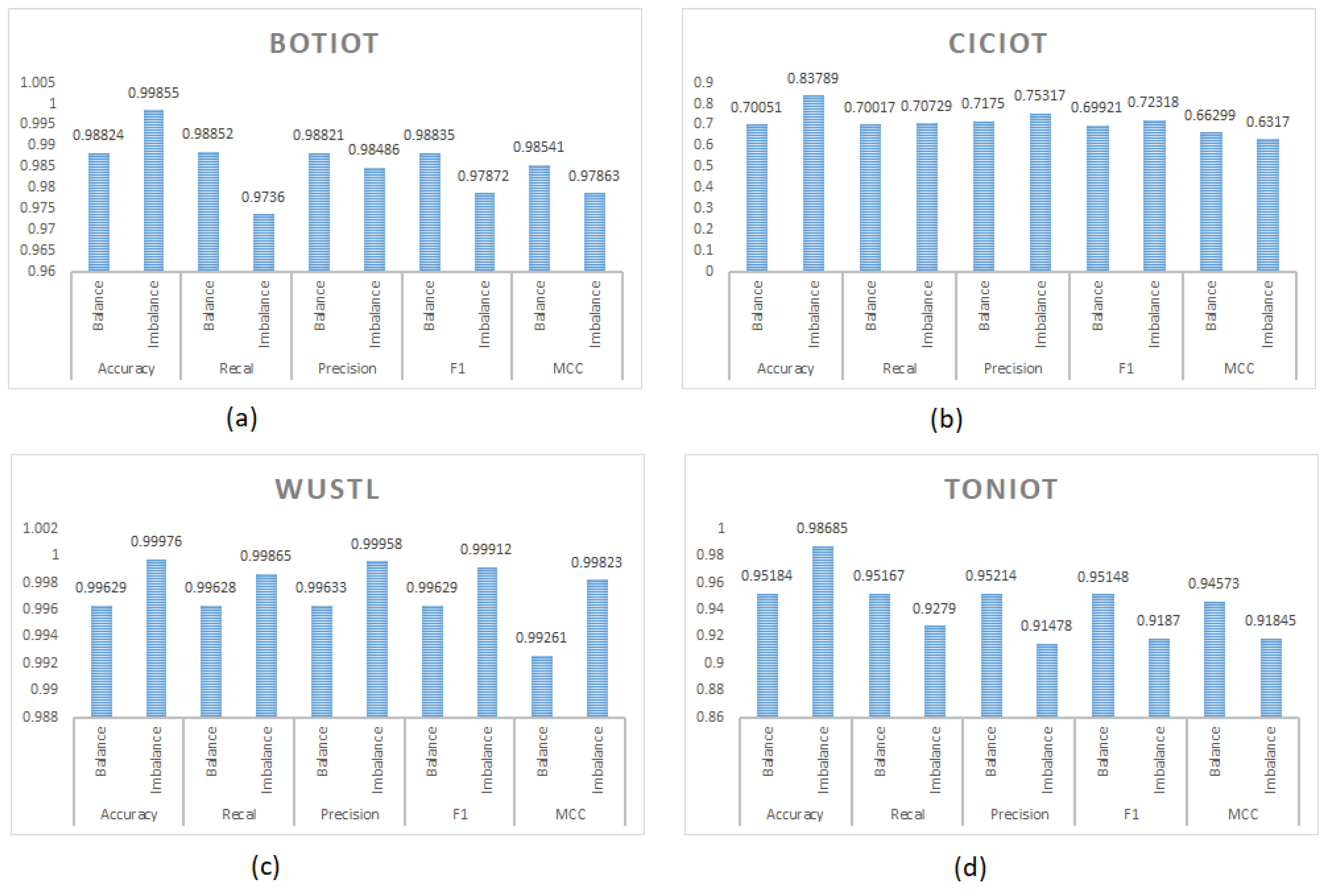
Data imbalance is a common challenge in many machine learning tasks, particularly in domains like intrusion detection where certain classes of data are significantly underrepresented compared to others. To address this issue and ensure fair model training, we employed a data balancing technique known as undersampling in our study. The undersampling reduces the number of samples in the majority class to achieve the balanced class distribution. In our experiments, the undersampling approach is chosen instead of oversampling (which balances the data by synthetic generation of samples) or duplication of existing samples to preserve the originality of the dataset. As a result, a balanced dataset is achieved while ensuring that the remaining samples in the class are still authentic and representative of the actual data distribution. The undersampling process involves careful selection of samples from categories with a higher number of instances and removing them until each category has a similar number of samples. This step is crucial to prevent bias and to maintain the integrity of the dataset. While undersampling helps to address the challenges of class imbalance, it also comes with considerations. One such consideration is the potential loss of information due to the removal of samples, which could impact the model’s ability to capture complex patterns in the data. In the context of deep learning techniques, data balancing through undersampling plays a vital role in improving model performance by reducing overfitting and ensuring a fair representation of all classes during training. By including this data balancing approach in our methodology, we aimed to enhance the robustness and accuracy of our deep learning-based intrusion detection system. The balanced datasets were subsequently split into 80% for training and 20% for testing. The resulting sample distribution is shown in

Table 1. Dataset split between training and testing samples after data balancing.

Dataset	Training Samples	Testing Samples
BoTIoT [23]	6312	1578
CiCIoT [24]	93,484	23,372
TonIoT [25,26]	52,416	13,104
WUSTL-IIoT-2021 [27]	139,226	34,806

.

4.1.2. Imbalanced Dataset

To ease the handling of the dataset, we extracted a portion of records of the original datasets, from which 80% is used for training and 20% is used for testing. This split was applied consistently across all datasets to ensure comparability in model evaluation. The number of records of minority class were not reduced. This decision was made to preserve the natural class imbalance present in real-world IoT traffic, where certain attack types are significantly underrepresented compared to others. While processing with imbalanced datasets, we used the 5% samples of each category of original datasets. This sampling strategy was adopted to reduce computational load while retaining representative distributions across classes. The sampling was applied uniformly, ensuring the overall class proportions remain unchanged. By maintaining the original imbalance in class distributions, this setup allowed us to evaluate how well each model performs under realistic data conditions. In such scenarios, performance metrics like recall and MCC become critical, particularly for identifying rare but high-impact attack types. For WUSTL-IIoT-2021, only binary classification is considered in the imbalanced setup as well, with ‘Normal’ and ‘Attacked’ categories. This dataset is included to examine performance under simpler class distributions and industrial IoT settings. The number of observations while performing the experiments on the imbalanced dataset are shown in

Table 2. Dataset records’ distribution for training and testing.

Dataset Name	Category Name	Original Records	Training Records	Testing Records
BoTIoT	Normal	9063	7250	1813
	Reconnaissance	1,789,474	71,578	17,895
	DoS	33,003,929	132,015	33,004
	Theft	1578	1262	316
	DDoS	38,531,238	154,125	38,531
CiCIoT	Benign Traffic	1,091,170	43,646	10,912
	DDoS	33,768,100	550,724	137,681
	DNS Spoofing	177,786	7111	1778
	Dictionary BruteForce	12,984	10,387	2597
	DoS	8,039,344	321,574	80,393
	Mirai	2,617,378	104,694	26,174
	Recon	352,244	41,795	10,449
	Web-based	24,658	19,726	4932
ToNIoT	Backdoor	508,116	20,324	5081
	DDoS	6,165,008	246,600	61,650
	DoS	3,375,328	135,013	33,753
	Injection	452,659	18,106	4526
	Password	1,718,568	68,742	17,186
	Ransomware	72,805	2912	728
	Scanning	7,140,161	285,606	71,402
	XSS	2,108,944	84,358	21,089
	Normal	796,380	31,855	7964
WUSTL-IIoT-2021	Normal	1,107,448	885,958	221,490
	Attacked	87,016	69,613	17,403

.

4.2. Dataset Details and Comparison

The experiments conducted in this study utilize four key datasets: BoTIoT [23], ToNIoT [25,26], CiCIoT [24], and WUSTL-IIoT-2021 [27]. Each dataset provides distinct insights into IoT and IIoT security challenges.

The BoTIoT dataset is built upon a realistic IoT network testbed designed at the University of New South Wales (UNSW), Australia, to simulate a smart home and smart city IoT environment. The testbed integrates multiple IoT devices and services with normal and malicious traffic streams to capture comprehensive network activity for intrusion detection research. The network consists of normal IoT devices, such as smart fridges, smart thermostats, smart garage doors, and surveillance cameras, all connected through a software-defined networking (SDN) environment to reflect modern IoT deployment models. These devices interact with remote cloud services via edge and gateway nodes, simulating real-world network behavior under normal operations. To generate malicious traffic, the environment includes simulated attack tools like Hping3, Slowloris, and Nmap, which are used to perform a variety of cyberattacks. These attacks are launched from compromised virtual machines within the network to mimic attacker behavior targeting the IoT infrastructure. The publicly available dataset is composed of multiple features and includes both training and testing subsets with detailed distributions of data items for different attack types.

The IoT network scenario in ToNIoT simulates a smart industrial environment composed of multiple interconnected devices, services, and operating systems. These include IoT/IIoT sensors and actuators (temperature, motion, humidity sensors), edge devices and gateways, operating systems (Windows 7, Windows 10, Ubuntu, and Android), and network infrastructure components. These entities are connected through a network topology that mirrors a smart manufacturing environment. The devices generate telemetry and communication data during normal operations and under various cyberattack scenarios. The attack traffic in the dataset is generated using tools such as Metasploit, Hping3, Nmap, GoldenEye, and Loic. The ToNIoT dataset incorporates diverse data sources from telemetry datasets of IoT and IIoT sensors, operating systems datasets, and network traffic datasets. It was collected from a network at the Australian Defence Force Academy, encompassing various virtual machines and hosts running different operating systems. This dataset includes many attack methods such as DoS, DDoS, and ransomware, against web apps, IoT gateways, and computer systems, thus providing a rich resource for developing intrusion detection systems.

The CiCIoT dataset was created by the Canadian Institute for Cybersecurity and is designed for deep learning-based intrusion detection in IoT contexts. The dataset is based on a smart home testbed environment that includes 105 IoT devices such as smart thermostats, lights, and cameras. These devices communicate through a Wi-Fi router to simulate real-world consumer IoT setups. The dataset captures both benign and malicious traffic to enable comprehensive evaluation of intrusion detection models in home IoT networks.

The WUSTL-IIoT-2021 dataset is developed by Washington University in St. Louis. The dataset includes telemetry data, network traffic data, and system logs. The testbed was developed by connecting industrial sensors and Programmable Logic Controllers (PLCs) using industrial protocols (e.g., Modbus/TCP) and edge computing gateways. The dataset collected from the testbed emulates the industrial IoT environment. This dataset supports binary classification by capturing normal and attack traffic flows, including unauthorized access and protocol misuse. Hence, it provides a comprehensive resource for analyzing device behavior in industrial settings.

The comparison of various features of datasets is crucial for evaluating the performance of the deep learning models in IoT-based intrusion detection systems.

Table 3. Comparison of datasets.

Datasets/Parameters	BoTIoT	CiCIoT	ToNIoT	WUSTL-IIoT-2021
No. of Samples	73,335,282	46,389,254	22,339,021	1,194,464
Number of Features	32	46	42	35
Number of Classes	5	9	10	2
Class Imbalance	Yes	Yes	Yes	Yes
Feature Variability	High	Moderate	High	Moderate
Statistical Properties	Varied	Varied	Varied	Varied
Contextual Usage	IoT Security	IoT Security	Industrial IoT Security	Industrial IoT Security
Scenario Suitability	Suitable for evaluating model scalability	Suitable for feature engineering	Beneficial for models with fewer samples	Diverse dataset for robust testing

compares these four datasets presented in this work, considering a variety of parameters.

4.3. Performance Metrics

The performance metrics taken into account when assessing the performance of our intrusion detection models are discussed below.

4.3.1. Accuracy

Accuracy is one of the indicators used to predict the perfection of the model. It reflects the percentages of accuracy of the values which were correctly classified in relation to the total number of cases in the dataset. When the data is not balanced, a better accuracy implies that the predictive results of the model are more accurate; however, it may not be enough to provide a complete picture of the performance of the model.

4.3.2. Recall

Another important measure of the functioning of the intrusion detection system is called recall. The recall value determines the ratio of successful accurate detection (true positives) of the model. Good recall provides a guarantee that real threats are not overlooked, which is critical parameter in cybersecurity applications, since failures to detect the intrusion can result in extensive damage.

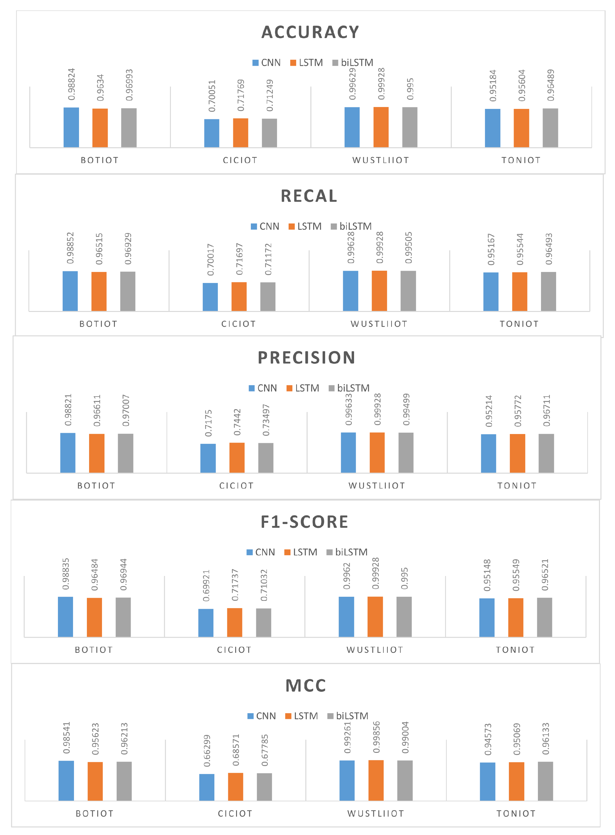
4.4. Precision

Precision is another metric used to evaluate the performance of a machine learning model. It refers to the quality of the positive predictions. Precision is the number of true positives divided by the overall number of positive predictions (i.e., the sum of true positives and false positives). In an IDS, the high precision indicates that if the system flags an event as an attack, it is more likely to be a genuine attack and less likely to be a harmless event (false alarm).

4.4.1. F1 Score

The F1 score is a balanced metric that takes into account both precision and recall. It provides a single figure that shows the trade-off between false positives and false negatives. It is computed as the harmonic mean of precision and recall. Recall and precision are better balanced when the F1 score is higher.

4.4.2. MCC (Matthews Correlation Coefficient)

False positives, false negatives, true positives, and true negatives are all taken into consideration by the Matthews correlation coefficient (MCC). It offers a fair assessment of the model’s effectiveness. The MCC metric is important specifically for the cases when there is an imbalance between the classes. The MCC metric is a number between −1 and 1, where 1 denotes ideal forecasts, 0 represents random predictions, and −1 denotes total discrepancy between predictions and actual results.

5. Results and Discussion

In this section, we demonstrate and explain the performance of the CNN, LSTM, and biLSTM models presented in Section 3.2 on the datasets discussed in above sections. For all of these models, three loss functions (cross-entropy, focal loss, and dual focal loss) are tested. To validate our results, we repeated all experiments multiple times with different random seeds and the average values of the performance parameters are reported. Furthermore, we benchmarked our models against baseline methods from the existing literature [28], demonstrating clear improvements in accuracy, recall, and MCC.

5.1. Comparison of Loss Function Performance

5.1.1. Balanced BoTIot Dataset

The results in

Table 4. Performance metrics for DL models with different loss functions for the BoTIoT balanced dataset.

DL Model	Loss Func	Acc	Recall	Prec	F1 Score	MCC
CNN	Cross	0.98824	0.98852	0.98821	0.98835	0.98541
	FL	0.98301	0.98352	0.98312	0.98331	0.97904
	DFL	0.98431	0.98465	0.98441	0.98431	0.98055
LSTM	Cross	0.9634	0.96515	0.96611	0.96484	0.95623
	FL	0.96667	0.96708	0.9686	0.96753	0.95937
	DFL	0.96797	0.96933	0.97144	0.96877	0.962
biLSTM	Cross	0.96209	0.96476	0.96281	0.96326	0.95411
	FL	0.95033	0.94943	0.95303	0.94991	0.93853
	DFL	0.96601	0.9668	0.97088	0.96761	0.95999
FNN-Rand [28]	FL	0.8614	0.4990	0.4990	0.5275	0.7623
FNN-CTGAN [28]	FL	0.8808	0.8652	0.4991	0.5540	0.7885
CNN-Rand [28]	FL	0.8084	0.7843	0.5349	0.5680	0.6550
CNN-CTGAN [28]	FL	0.8168	0.7988	0.4298	0.4536	0.6878

highlight a key contrast between the data-balancing strategies used in this study and those in the baseline models from [28]. While the baseline models rely on oversampling techniques either through random duplication (Rand) or synthetic data generation using CTGAN, the models in this study use undersampling to achieve a balanced dataset.

The findings indicate that undersampling led to significantly better model performance across all deep learning architectures. For instance, the CNN model trained with cross-entropy loss in this study achieved an accuracy of 0.98824 and an MCC of 0.98541. This notable performance of CNN can be explained by BoTIoT’s high-dimensional structured feature space, which benefits from CNN’s capacity to learn spatial hierarchies. The model effectively captured local interactions among features that are crucial for distinguishing between attack classes. In comparison, the best-performing CNN baseline (CNN-CTGAN) achieved only 0.8168 accuracy and 0.6878 MCC, suggesting that oversampling with synthetic data may have introduced noise or redundant patterns, thereby hindering the model’s ability to generalize effectively. Additionally, the precision of the CNN-CTGAN model (0.4298) is significantly lower than any CNN variant in this study, further indicating that the synthetic data generation may have negatively affected class separation.

Similarly, the LSTM and biLSTM models trained on undersampled data showed superior performance compared to the baseline models that used oversampling. The LSTM model with DFL, for instance, achieved an accuracy of 0.96797 and an MCC of 0.962, whereas the best FNN-based model from the baseline (FNN-CTGAN) had only 0.8808 accuracy and 0.7885 MCC. The recall values in this study are also consistently higher, indicating that the undersampled models retained strong sensitivity to minority class instances without the risk of overfitting to synthetic patterns.

One of the key weaknesses of the oversampling approach used in the baseline study is evident in the MCC values. MCC is particularly important in imbalanced datasets as it considers both false positives and false negatives. The fact that the highest MCC in the baseline study (0.7885 for FNN-CTGAN) is significantly lower than those in this study (e.g., CNN with cross-entropy: 0.98541, LSTM with DFL: 0.962) demonstrates that undersampling led to a better overall decision boundary.

5.1.2. Balanced CiCIoT Dataset

When evaluating the CiCIoT dataset shown in

Table 5. Performance metrics for DL models with different loss functions for the CiCIoT balanced dataset.

DL Model	Loss Func	Acc	Recall	Prec	F1 Score	MCC
CNN	Cross	0.69622	0.69592	0.71519	0.69429	0.65842
	FL	0.69815	0.69833	0.70869	0.69828	0.65854
	DFL	0.7033	0.70348	0.72331	0.70181	0.66727
LSTM	Cross	0.71769	0.71697	0.7442	0.71737	0.68571
	FL	0.69252	0.69309	0.71396	0.69414	0.6564
	DFL	0.71264	0.71066	0.73351	0.70924	0.67643
biLSTM	Cross	0.71249	0.71172	0.73497	0.71032	0.67785
	FL	0.71004	0.71161	0.73743	0.7098	0.67826
	DFL	0.707	0.70727	0.73558	0.70531	0.67384

, we noted that the CNN model achieved the best performance with DFL, displaying high accuracy, recall, precision, F1 score, and MCC. Cross-entropy loss and FL also performed well, indicating that CNNs are versatile across different loss functions. On the other hand, the LSTM and biLSTM models exhibited strong performance with all loss functions, with cross-entropy loss providing the best balance of accuracy and MCC. This robustness indicates that LSTM-based architectures are well suited for the CiCIoT dataset, regardless of the loss function used.

5.1.3. Balanced WUSTL-IIOT-2021 Dataset

The analysis of DL models on the WUSTL-IIOT-2021 dataset (

Table 6. Performance metrics for DL models with different loss functions for the WUSTIIoT balanced dataset.

DL Model	Loss Func	Acc	Recall	Prec	F1 Score	MCC
CNN	Cross	0.99629	0.99628	0.99633	0.99629	0.99261
	FL	0.99638	0.99638	0.9964	0.99638	0.99278
	DFL	0.99601	0.99599	0.99604	0.99601	0.99204
LSTM	Cross	0.99928	0.99928	0.99928	0.99928	0.99856
	FL	0.99851	0.9985	0.99851	0.99851	0.99701
	DFL	0.99914	0.99914	0.99914	0.99914	0.99828
biLSTM	Cross	0.995	0.99505	0.99499	0.995	0.99004
	FL	0.99839	0.99839	0.99839	0.99839	0.99678
	DFL	0.99879	0.9988	0.99879	0.99879	0.99759

) shows that CNN performs exceptionally well across metrics, with FL being slightly better than cross-entropy and DFL. This showcases the CNN’s effectiveness with complex data regardless of the loss function used. LSTM excels with cross-entropy, highlighting its superior generalization, while biLSTM performs remarkably with specialized loss functions, emphasizing their role in handling class imbalances effectively.

5.1.4. Balanced ToNIoT Dataset

In

Table 7. Performance metrics for DL models with different loss functions for the ToNIoT balanced dataset.

DL Model	Loss Func	Acc	Recall	Prec	F1 Score	MCC
CNN	Cross	0.95184	0.95167	0.95214	0.95148	0.94573
	FL	0.94597	0.94624	0.94705	0.94611	0.93969
	DFL	0.95787	0.95798	0.95837	0.95809	0.95288
LSTM	Cross	0.95604	0.95544	0.95772	0.95549	0.95069
	FL	0.94108	0.94046	0.94152	0.94041	0.93342
	DFL	0.91926	0.91894	0.9253	0.92003	0.91125
biLSTM	Cross	0.96489	0.96493	0.96711	0.96521	0.96133
	FL	0.95871	0.95879	0.9588	0.95835	0.95348
	DFL	0.96657	0.96679	0.96713	0.96659	0.96264

, we present the performance comparison of proposed DL algorithms for different loss functions on the ToNIoT dataset. For the ToNIoT dataset, the results are similar to the other datasets. Similar to the other datasets, the CNN model shows solid performance across all metrics and loss functions. Using cross-entropy loss, CNN achieves high accuracy, precision, and F1 score. Focal loss results in slightly lower accuracy, which indicates that FL faces challenges in handling balanced data effectively. For this dataset, the CNN and biLSTM models exhibit robust performance across all loss functions, with DFL providing a slight edge in precision and accuracy. The LSTM model performs exceptionally well with cross-entropy loss as compared to FL and DFL.

5.2. Comparison of the Performance of Various DL Models

A performance analysis of the deep learning models across the four IoT datasets is shown in Figure 1. The results demonstrate that the CNN model consistently performs well across all datasets. This superior performance can be attributed to CNN’s ability to capture high-dimensional spatial features, which are typically present in IoT environments, effectively. The high accuracy, recall, precision, F1 score, and MCC metrics for these datasets indicate that CNNs are adept at distinguishing between different classes of data having complex patterns and noise; CNNs handle these well through convolutional layers.

The LSTM and biLSTM models demonstrate strong performance on the WUSTL-IIoT-2021 dataset. The results suggests that these models are effective in handling sequential data and capturing long-term dependencies. This capability is crucial in IoT environments where data streams are continuous. On the other hand, the performance of LSTM and biLSTM is lower on the CiCIoT dataset than CNN. This is due to the dataset characteristics that favor the spatial feature extraction strength of CNNs more than the temporal handling of LSTMs. The analysis and the performance trends indicate that for datasets that contain rich spatial features like BoTIoT and CiCIoT, CNNs are highly effective. Meanwhile, for datasets that include significant sequential data or require handling of long-term dependencies, as present in WUSTL-IIoT-2021, LSTMs and biLSTMs are more suitable than CNNs.

5.3. Analysis for Imbalanced Dataset

5.3.1. Comparison of DL Models

The evaluation of CNN, LSTM, and biLSTM models across different IDS datasets reveals insightful trends in performance as shown in

Table 8. Performance analysis of CNN, LSTM, and biLSTM models on IDS datasets.

Model	Dataset	Accuracy	Recall	Precision	F1-Score	MCC
CNN	BoTIoT	0.99855	0.9736	0.98486	0.97872	0.97863
	CiCIoT	0.83789	0.70729	0.75317	0.72318	0.66299
	WUSTIIoT	0.99976	0.99865	0.99958	0.99912	0.99823
	ToNIoT	0.98685	0.9279	0.91478	0.9187	0.91845
LSTM	BoTIoT	0.99392	0.97141	0.98116	0.97617	0.97414
	CiCIoT	0.90673	0.90946	0.88384	0.89454	0.87181
	WUSTIIoT	0.99926	0.99523	0.99931	0.99726	0.99453
	ToNIoT	0.9891	0.94379	0.94053	0.94164	0.9406
biLSTM	BoTIoT	0.98993	0.81711	0.98474	0.83575	0.85839
	CiCIoT	0.82907	0.66702	0.75991	0.68618	0.66583
	WUSTIIoT	0.99977	0.9988	0.99951	0.99915	0.99831
	ToNIoT	0.98964	0.89913	0.93475	0.90852	0.91123

and

Table 9. Performance metrics of different models on IDS imbalanced datasets.

Metric	Model	BoTIoT	CiCIoT	WUSTIIoT	ToNIoT
Accuracy	CNN	0.99855	0.83789	0.99976	0.98685
	LSTM	0.99392	0.90673	0.99926	0.9891
	biLSTM	0.98993	0.82907	0.99977	0.98964
Recall	CNN	0.9736	0.70729	0.99865	0.9279
	LSTM	0.97141	0.90946	0.99523	0.94379
	biLSTM	0.81711	0.66702	0.9988	0.89913
Precision	CNN	0.98486	0.75317	0.99958	0.91478
	LSTM	0.98116	0.88384	0.99931	0.94053
	biLSTM	0.98474	0.75991	0.99951	0.93475
F1 Score	CNN	0.97872	0.72318	0.99912	0.9187
	LSTM	0.97617	0.89454	0.99726	0.94164
	biLSTM	0.83575	0.68618	0.99915	0.90852
MCC	CNN	0.97863	0.66299	0.99823	0.91845
	LSTM	0.97414	0.87181	0.99453	0.9406
	biLSTM	0.85839	0.66583	0.99831	0.91123

. CNN achieves consistently high accuracy across datasets, with the best performance on WUSTIIoT (Accuracy: 0.99976, F1-Score: 0.99912, MCC: 0.99823). However, CiCIoT remains a challenging dataset, where CNN shows a drop in accuracy (0.83789) and F1 score (0.72318), indicating difficulty in handling this dataset’s complexity.

LSTM shows superior recall values compared to CNN, particularly for CiCIoT, indicating better performance in detecting minority class instances. This suggests that the sequential nature of LSTM helps in identifying attack patterns over time. Additionally, WUSTIIoT achieves near-perfect classification. However, for datasets like ToNIoT, the improvement over CNN is marginal, suggesting that temporal dependencies in attack detection are less pronounced for this dataset.

The biLSTM model demonstrates mixed performance, showing some improvements in accuracy but a notable drop in recall for the BoTIoT and CiCIoT datasets. This reduction in recall may be attributed to the presence of overlapping or sparse temporal patterns in these datasets, which can hinder the model’s ability to effectively capture sequential dependencies. Although biLSTM maintains relatively high precision, the lower recall indicates challenges in generalizing temporal features across all classes. In contrast, on the WUSTL-IIoT dataset, biLSTM achieves the highest overall performance, highlighting its effectiveness in handling more structured and temporally consistent data.

After analyzing the results, we can conclude that CNN performs well across most datasets but struggles with CiCIoT, where LSTM provides better recall value. LSTM consistently delivers strong results, while biLSTM offers marginal improvements for certain datasets but struggles with recall. Therefore, the choice of model depends on the dataset’s characteristics, with LSTM being preferable for datasets with temporal dependencies and CNN excelling in structured datasets.

5.3.2. Comparison of Loss Functions

In this section, we provide the analysis of different loss functions on intrusion detection models to provide insights into their effectiveness across various datasets.

We can see from

Table 10. Performance analysis of different loss functions.

Loss Function	Dataset	Accuracy	Recall	Precision	F1-Score	MCC
Cross	BoTIoT	0.99855	0.9736	0.98486	0.97872	0.97863
	CiCIoT	0.83789	0.70729	0.75317	0.72318	0.66299
	WUSTIIoT	0.99976	0.99865	0.99958	0.99912	0.99823
	ToNIoT	0.98685	0.9279	0.91478	0.9187	0.91845
FL	BoTIoT	0.99735	0.96956	0.97854	0.97387	0.97319
	CiCIoT	0.82652	0.67748	0.74173	0.69503	0.69503
	WUSTIIoT	0.99953	0.99753	0.99894	0.99824	0.99647
	ToNIoT	0.98333	0.89975	0.90873	0.90393	0.90214
DFL	BoTIoT	0.99778	0.97481	0.98437	0.97949	0.97889
	CiCIoT	0.82854	0.67455	0.75104	0.69226	0.66916
	WUSTIIoT	0.99981	0.99889	0.99971	0.9993	0.9986
	ToNIoT	0.98232	0.90509	0.90162	0.90219	0.90072

that the cross-entropy (CE) loss performs well overall as compared to other loss functions by achieving the highest accuracy for WUSTIIoT and BoTIoT, along with strong precision and recall values. However, it struggles with CiCIoT, where accuracy drops to 0.83789 and the F1 score is relatively lower, indicating challenges in handling class imbalance.

Focal loss (FL), which is designed to address class imbalance by reducing the weight of well-classified instances and focusing on hard-to-classify cases, improves recall in CiCIoT; however, it does not significantly improve accuracy and even reduces precision compared to CE. On the other hand, on the WUSTL-IIoT dataset, FL performs better, showing some performance gains over CE. However, for ToNIoT, FL results in a slightly lower accuracy and MCC than CE.

Dual focal loss (DFL) results in the best overall accuracy for WUSTIIoT and BoTIoT, along with the highest precision values. However, DFL does not significantly improve CiCIoT performance, where the accuracy remains close to FL. The impact of DFL is more visible in datasets with balanced distributions, whereas its benefits for handling imbalanced datasets such as CiCIoT are marginal. Although DFL is designed to enhance performance on imbalanced datasets, its limited improvement on CiCIoT stems from high inter-class similarity and feature overlap among attack types. In such cases, loss function tuning alone does not yield significant performance gains without additional feature engineering or model complexity.

5.4. Effects of the Data-Balancing Technique

The impact of data balancing through undersampling significantly influences the performance of IDS models across different datasets, as shown in Figure 2. In general, imbalanced datasets exhibit higher accuracy compared to their balanced counterparts. This trend is particularly evident in the BotIoT and WUSTL datasets, where accuracy remains consistently high even when balancing is applied. However, the CiCIoT dataset experiences a substantial accuracy drop when balanced (0.70051 vs. 0.83789 in the imbalanced case), suggesting that balancing increases classification difficulty due to higher class overlap or insufficient attack representation in the reduced dataset.

A deeper look into recall values reveals that BotIoT and WUSTL maintain high recall scores across both balanced and imbalanced datasets, indicating the suitability of the models for detecting attacks in these environments. However, CiCIoT exhibits a lower recall value when balanced using undersampling. This pattern suggests that while undersampling can correct biases in heavily skewed datasets, it may also eliminate essential attack instances for some datasets and can affect the model’s generalization ability.

Analyzing the results of precision, we can see that imbalanced datasets generally achieve higher precision scores, particularly in the WUSTL dataset. However, CiCIoT and TONIoT datasets show precision losses after balancing, which imply that the models struggle with attack class discrimination when fewer training samples are available. This precision drop is also reflected in the F1 score, where CiCIoT reaches only 0.69921 under balanced conditions, reinforcing the difficulty of making accurate attack predictions with a reduced dataset.

We also evaluate the MCC scores to highlight the overall reliability of the models. We can see that WUSTL dataset shows the most stable results for MCC. The MCC for CiCIoT drops when balanced, indicating that undersampling does not significantly improve classification reliability for this dataset. This suggests that removing excess data from the majority class does not always lead to better classification performance, especially when the dataset structure is complex.

6. Conclusions

In this study, we conducted a comprehensive performance analysis of three deep learning models (CNN, LSTM, and biLSTM) on four datasets (BoTIoT, CiCIoT, ToNIoT, and WUSTL-IIOT-2021) using three distinct loss functions (cross-entropy, focal loss, and dual focal loss). We have shown that data balancing through undersampling is more effective as compared to data balancing through oversampling and the synthetic generation of data. Moreover, the findings indicate that CNN is effective compared to LSTM and biLSTM model on all datasets, whereas LSTM and biLSTM are effective in the datasets with a temporal character. Such higher performance is explained by the fact that CNN has a greater capacity to capture complex features, which are essential in situations concerning IoT-based intrusion detection systems. In the future, we aim to explore how combining the spatial feature extraction capabilities of CNNs with the temporal analysis strengths of LSTMs can enhance detection performance in more complex IoT settings. The interpretability of models can also help in practical deployment via methods such as SHAP or LIME. Lastly, testing each of the models under time restrictions would assist in determining their practicability and feasibility of installation in edge-based or cloud-encompassing IoT security protocols.