Fair and Explainable Multitask Deep Learning on Synthetic Endocrine Trajectories for Real-Time Prediction of Stress, Performance, and Neuroendocrine States

Abstract

Cortisol and testosterone are key digital biomarkers reflecting neuroendocrine activity across the hypothalamic–pituitary–adrenal (HPA) and hypothalamic–pituitary–gonadal (HPG) axes, encoding stress adaptation and behavioral regulation. Continuous real-world monitoring remains challenging due to the sparsity of sensing and the complexity of multimodal data. This study introduces a synthetic sensor-driven computational framework that models hormone variability through data-driven simulation and predictive learning, eliminating the need for continuous biosensor input. A hybrid deep ensemble integrates biological, behavioral, and contextual data using bidirectional multitask learning with one-dimensional convolutional neural network (1D-CNN) and long short-term memory (LSTM) branches, meta-gated expert fusion, Bayesian variational layers with Monte Carlo Dropout, and adversarial debiasing. Synthetically derived longitudinal hormone profiles that were validated by Kolmogorov–Smirnov (KS), Wasserstein, maximum mean discrepancy (MMD), and dynamic time warping (DTW) metrics account for class imbalance and temporal sparsity. Our framework achieved up to 99.99% macro F1-score on augmented samples and more than 97% for unseen data with ECE below 0.001. Selective prediction further maximized the convergence of predictions for low-confidence cases, achieving 99.9992–99.9998% accuracy on 99.5% of samples, which were smaller than 5 MB in size so that they can be employed in real time when mounted on wearable devices. Explainability investigations revealed the most important features on both the physiological and behavioral levels, demonstrating framework capabilities for adaptive clinical or organizational stress monitoring.

1. Introduction

Using wearable sensors, synthesized hormonal data, and multitask deep learning, this work presents the first real-time human-centric model to predict neuroendocrine, stress, cognitive and emotional states for intelligent interventions in personalized health and performance monitoring. Cortisol and testosterone at the molecular level both express circadian rhythms under the control of the HPA axis and the HPG axis, respectively [1,2], and rapidly respond to an acute stressor, but gradually recover toward a baseline afterward [3,4]. Alterations of these rhythms are associated with risk for cardiovascular, metabolic, reproductive, and neuropsychiatric dysfunction [5,6]. Modeling timely changes in biomarkers enables them to serve as early warnings of molecular deregulation, hence predicting disease onset [7].

Employee well-being, cognitive performance, and physiological health are mutually dependent in organizational settings, all of which are essential to productivity and resilience [8]. More than 75% of workers have chronic stress [9], and it deteriorates focus, memory, and decision-making skills [10], and hormone imbalances make these worse [11]. These disruptions drive absenteeism, presenteeism, low job satisfaction, and healthcare costs [12,13,14], in turn reducing the productivity of the workforce by  20% [15,16] and the burden of obesities/heart diseases [17]. Early and accurate detection of stress and hormone deviations is crucial for timely interventions aimed at optimizing organizational health [18].

Standard monitoring depends on behavioral indicators or self-reports [19] or single-point hormone measurements [1,3], which do not show circadian rhythms or sudden spikes [2,4], making personalized predictions less accurate [20]. These gaps underscore the necessity for integrative frameworks that amalgamate multimodal biological, behavioral, and contextual data to dynamically and interpretively predict stress, performance, and hormonal health [7,8].

Machine learning and synthetic data generation offer scalable methodologies to model these interactions longitudinally, facilitating the early identification of risk states and the development of fairness-conscious intervention strategies [11,12]. However, current models frequently exhibit deficiencies in interpretability, demographic equity, resilience to deployment limitations, and biologically plausible synthetic augmentation, thereby constraining their capacity to accurately represent temporal hormone dynamics [16,17].

There are still two issues with wearable technology: class imbalance for clinically significant states like “Critical” stress and biosensing sparsity (few hormone samples per subject), which hinders direct time-series learning. To overcome those issues, this work (A) proposes biologically constrained synthetic longitudinal hormone trajectories anchored to per-subject measures [18,19,20]. This allows for temporal modeling without the need for continuous biosensors, and (B) creates a hybrid, uncertainty-aware multitask pipeline that enhances minority-class detection, quantifies predictive uncertainty for selective human review, and provides understandable explanations for interventions. Specifically, we aim to develop a reproducible synthetic augmentation pipeline that maintains per-subject correlations, assess performance in both augmented and real-only scenarios, quantify calibration and fairness, and quantify interpretability using quantitative explainability metrics.

We introduce a hybrid deep ensemble framework designed to predict stress, performance, and hormonal health by modeling physiological, behavioral, and contextual interactions. A bidirectional multitask architecture learns both shared and task-specific representations, while a temporal branch uses convolutional and recurrent layers to capture changing hormone trajectories. Meta-gated expert fusion, which adaptively chooses relevant biological or behavioral modules for each sample, and adversarial debiasing, which reduces differences between groups of people, making sure that the system is fair and easy to understand. Bayesian layers and ensemble strategies give us calibrated uncertainty estimates that we can trust when using them in sensitive real-world situations.

2. Key Contributions

• We propose a deep ensemble model that combines biological, behavioral, and synthetic longitudinal hormone data in a bidirectional multitask framework to make concurrent interpretable predictions for stress, performance, and hormone health.
• A temporal branch based on 1D CNN and long short-term memory (LSTM) layers to learn dynamic changes of hormones, enhancing sensitivity towards important temporal patterns.
• A meta-gating strategy to dynamically select expert modules for samples, thus improving modular interpretability and individualized decision-making.
• We leverage adversarial debiasing to mitigate demographic biases, and for uncertainty-aware predictions, we combine Bayes Layers with multimodality and MCP Dropout.
• For real-time deployment, compact sizes (<5 MB) and low latencies (<20 ms) are provided, as well as continuous monitoring and state-of-the-art performance with explainability have been reported in terms of SHAP and counterfactual analysis.

Our presented methods reconcile ML and healthcare, offering a scalable, interpretable, fair, and uncertainty-aware approach to real-time health monitoring through wearables and mobile devices. By combining biological fidelity and predictive analytics, this work contributes to the development of reliable AI solutions in organizational health management. This is how the paper is written in order: in Section 2, we look at related work; in Section 3, we talk about the dataset and synthetic hormone augmentation; in Section 4, we talk about the hybrid model and training; in Section 5, we show the results; in Section 6, we talk about the implications; and in Section 7, we end.

3. Related Work

Wearables, hormone modeling, and advanced machine learning have driven personalized health tracking, with high-fidelity analysis of stress [21,22], and aging [23], as well as circadian rhythmicity [24]. Wearable devices enable continuous and minimally intrusive physiological and behavioral monitoring, with unmatched temporal resolution. Multimodal data-driven machine learning methods have increased the use of predictive modeling for complex biological and psychological phenomena. Even non-human studies show the potential of hormone-dependent stress phenotyping, such as fish models, indicating cortisol and other biomarkers in the response to distress [25]. Synthetic longitudinal health datasets also promote simulation and predictive modeling, allowing comprehensive evaluation of machine learning models [26]. Integrative methods that incorporate genetics, hormonal profiles, or brain function have revealed the complexity of conditions such as psychiatric disorder depression—a testament to the need for multimodal and longitudinal data in predictive ability [27,28,29].

In medical applications, uncertainty-aware deep learning has gained attention due to its ability to provide well-calibrated confidence with the predictions for diabetic retinopathy classification or early cancer detection [30,31]. Analytical research investigating specific hormones has highlighted the role of testosterone and cortisol in precision medicine, personalized treatments, and health optimization programs [32,33]. Recent developments also comprise interpretable and causal ML frameworks for making actionable decisions by focusing on counterfactual reasoning, fairness, etc. [34].

Moreover, digital biomarkers and minimally invasive longitudinal monitoring methodologies also drive scalable health assessment [35]. Real-time prediction of wearable physiological stress supports the potential for continuous monitoring of context-sensitive settings in dynamic settings [36,37]. The companion methodological contributions of kernel-based tests for dependent sequential data and multitask LSTM models for personalizing interventions have enhanced robust inferential ability and time-series modeling [38,39].

Together, these papers demonstrate important advances in the development of wearable devices that connect with hormone dynamics and sophisticated ML methods. Yet, major gaps exist in models that have multi-hormonal joint modeling capability in a multitask, interpretable, and uncertainty-aware manner, and which can effectively utilize all forms of longitudinal information according to their modalities. Current wearable and machine learning (ML)-based stress/prediction efforts usually use sparse or cross-sectional single-point hormone measures that miss transient and circadian stress dynamics, ignore demographic confounding, or only use ad hoc fairness checks. They also only offer an inadequate quantitative assessment of the fidelity of synthetic data (few report KS/MMD/DTW statistics).

In small-sample cohorts, these restrictions impair clinical interpretability and generalizability. To fill these gaps, our pipeline incorporates adversarial debiasing, sets up per-subject anchoring during augmentation, explicitly models dual-hormone temporal trajectories (cortisol and testosterone), and reports statistical fidelity tests (KS, Wasserstein, MMD, DTW) and held-out real-only evaluations. A logic-progression approach may help bridge these gaps to translate predictable intuition into robust and ethical medical decision-making.

4. Research Methodology

We propose a deep mixed ensemble that integrates biological, behavioral, and contextual signals for stress, performance, and hormone health prediction. The dataset consists of hormone and behavior data measured using a validated assay for cortisol and testosterone. Instead of designing new hardware, the research constructs a processing infrastructure that converts conventional biosensor signals to actionable digital biomarkers using sophisticated mathematical analysis, so the system can be easily interfaced with prospective wearable platforms for hormone monitoring in real-time. The bidirectional multitask allows back-and-forward inference that increases the anatomical consistency and interpretability. A meta-gated expert network samples modalities around a sample, while adversarial debiasing, Bayesian ensembles, and Monte Carlo Dropout deliver calibrated, fairness-aware, and risk-conscious predictions. Longitudinal features extracted from synthetic 7-day cortisol and testosterone sequences are used as inputs to a 1D-CNN+LSTM-based temporal branch model, which captures spikes, slopes, and circadian dynamics. Class-aware sampling, focal loss, temperature scaling, and selective prediction deal with rare high-risk classes and uncertainty. SHAP attribution, meta-gating visualization, and counterfactual analysis offer an interpretable interface for agents. Our framework utilizes fairness-aware multitask learning, temporal biological fidelity, and uncertainty-informed decision support in a single, robust system.

We conducted a full demographic analysis to ensure fair representation across all groups. Appendix A presents the complete demographic distributions, cross-tabulations for all outcome labels, and statistical balance tests (chi-square/Fisher exact tests for categorical variables; ANOVA/Kruskal–Wallis tests for continuous variables with Benjamini–Hochberg FDR correction). No substantial demographic imbalance was observed, apart from a minor age-related effect, and subgroup analyses demonstrated uniform accuracy and Macro-F1 across demographic groups. We also assessed predictor importance using SHAP values, permutation importance, LASSO/ElasticNet stability selection, and RFE-CV. A compact set of approximately 8–15 predictors retained ≥92–$96\%$ of the full-model performance, with RFE curves plateauing near 15 features and stability coefficients $\ge 0.60$ indicating robust minimal sets. Appendix B provides the complete predictor rankings, stability analyses, and reduced-feature performance curves.

4.1. Dataset Overview

The primary dataset comes from the Columbia MBA Hormone Diversity Team Study, which includes 370 persons nested within 74 teams, from whom we have cortisol and testosterone levels in logarithmic transformations, demographics (age, gender, ethnicity, country), and team-level outcomes such as the following: performance, cash allocation in groups of four players playing a lenient contract of acceptall-or-rejectthedeal UG game [29], rank order and cooperation level, defined as the amount offered in each round in the repeated TG, where participants do not remember the last offer that was declined. One easy measure of group diversity is the number of unique gender-ethnicity-country combinations in a team, capturing intersectional heterogeneity [40,41]. Controlling for the three class outputs—Stress (cortisol), Performance (team results), and Hormone Health (testosterone) enabled both forward inference (biological + context to outcomes) and reverse inference (predicted outcomes to hormone health), thereby improving interpretability.

Hormone measurements (cortisol and testosterone) represented proxies for potential continuous monitoring output. The developed sensor-agnostic framework applies to microfluidic, electrochemical, and wearable biosensors for a flexible hormone inference from various forms of inputs. Other existing public datasets offer simultaneous longitudinal cortisol–testosterone with associated behavioral/contextual features. Therefore, synthetic enrichment is incorporated for generalization. This encompasses molecular and clinical data, hormone assays such as cortisol, estradiol, testosterone, insulin, thyroid hormones, routine biochemistry such as glucose, lipids, and liver/kidneys panels, and inflammatory markers CRP/interleukins measured by validated immunoassays or mass spectrometry. Combined with clinical covariates (age, BMI, comorbidity, and medication), these inputs provide sufficient context for accurate and interpretable models of biochemical status and physiological modifiers.

Dataset Structure and Fields

The primary dataset is the Columbia MBA Hormone Diversity Team Study, comprising 370 participants organized into 74 work teams (5 ± 2 members each). Each record corresponds to an individual participant observed within a specific team context. The dataset integrates biological, behavioral, and contextual modalities within a single relational schema, summarized below.

• Storage structure: A single flat table participants.csv with one row per subject, relationally linked to auxiliary JSON objects storing each subject’s temporal hormone traces and behavioral trajectories.
• Primary keys: subject_id (unique per participant) and team_id (linked to group-level performance indicators).
• Total observations: 370 rows ×∼45 columns (static attributes) plus two time-series arrays per subject (cortisol and testosterone, 168 samples each).
• Multimodal representation:

  -

  Static numerical: Age, BMI, baseline cortisol/testosterone (log-scaled).

  -

  Categorical/contextual: Gender, Ethnicity, Country (one-hot or trainable 8-dimensional embeddings).

  -

  Behavioral temporal: cash_trajectory and rank_trajectory (vectors of per-round outcomes).

  -

  Team-level features: diversity_index, team_performance_score.

  -

  Derived temporal features: cortisol_slope_am, t_react_recovery, stress_auc, hormone_entropy.

  -

  Synthetic augmentation metadata: augmentation_flag, synthetic_seed, and sequence_id (for reproducibility).

Each biological time-series was resampled to an hourly grid covering seven days (7 × 24 = 168 steps). Synthetic enrichment added physiologically constrained trajectories per subject while retaining baseline anchoring to maintain biological plausibility, as shown in

Table 1. Feature summary and counts for the Columbia MBA Hormone Diversity Team Study dataset.

Feature Type	Example Variables	Count	Representation/Range
Demographic (static)	age, gender, ethnicity, country, BMI	5	numeric/categorical (embedded)
Biological (static)	baseline_cortisol_log, baseline_testosterone_log	2	float (µg/dL, log-scaled)
Biological (temporal)	cortisol_series[168], testosterone_series[168]	2 × 168	float arrays (per hour)
Derived temporal features	cortisol_slope_am, t_react_recovery, stress_auc, hormone_entropy	4	float
Behavioral temporal	cash_trajectory[10], rank_trajectory[10]	2 × 10	float arrays
Contextual/team features	team_id, diversity_index, team_performance_score	3	numeric/categorical
Synthetic metadata	augmentation_flag, synthetic_seed, sequence_id	3	int/bool

.

Total feature dimensionality after preprocessing, approximately 40 static + (168 × 2) temporal channels, yielded 376 input dimensions per participant sample. Each row in the dataset corresponds to one participant (e.g., subject P0371 in team T062), containing demographic fields (age = 29, gender = female, ethnicity = Asian, BMI = 22.1), baseline hormone levels (baseline_cortisol_log = 0.54, baseline_testosterone_log = 0.71), and team-level indicators (team_performance_score = 0.83, diversity_index = 0.68). Derived temporal features such as cortisol_slope_am = 0.06, t_react_recovery = 2.7 h, and stress_auc = 0.42 summarize hormone dynamics. Behavioral trajectories such as cash allocations and rank order per round are stored as short numerical arrays as [105, 112, 118, …] and [3, 2, 1, …]; full arrays are available in the shared repository. The Boolean augmentation_flag indicates whether a sample is real (0) or synthetic (1), ensuring full traceability across cross-validation folds.

The real-world measurements originate from Hormones and the Dynamics of Team Performance, Open Science Framework Repository, OSF.IO/ZPQ8H. Raw saliva assays (cortisol, testosterone) were analyzed using validated enzyme-immunoassay protocols, and behavioral/demographic data were matched via anonymized identifiers. All preprocessing, resampling, and synthetic augmentation scripts are available in the project’s GitHub repository (see Data Availability Statement). Random seeds and augmentation parameters are logged per subject via synthetic_seed to ensure exact reproducibility.

4.2. Data Preprocessing and Cleaning

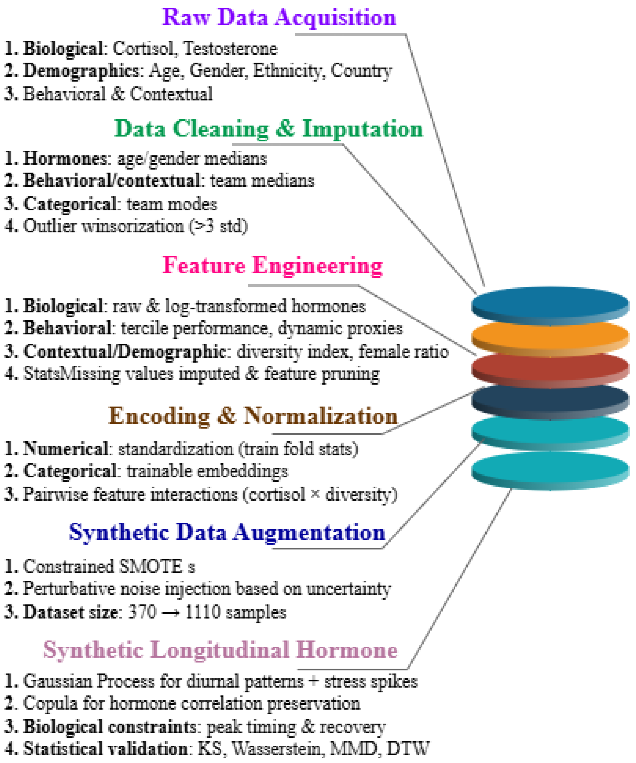
A rigorous preprocessing pipeline was applied to ensure high-quality static and temporal features for the hybrid multitask model. All steps were nested within a stratified 10-fold team-level cross-validation to prevent leakage. Hormone values of cortisol/testosterone were imputed using age- and gender-specific medians, behavioral/contextual features with team medians, and categorical variables such as ethnicity and country with team modes. Hormonal outliers beyond three standard deviations were winsorized as shown in Figure 1. Numerical features were standardized, categorical features encoded as 8-dimensional trainable embeddings, and behavioral features smoothed via exponential moving averages.

Temporal hormone dynamics were captured using 7-day (168-step) synthetic sequences, processed through a 1D-CNN (32 filters, kernel size 3) for spike detection and an LSTM (64 units) for recovery trends. Rare classes such as critical stress and low hormone health were balanced using SMOTE, with light Gaussian noise ($\sigma =0.01$) added to hormones for robustness. All preprocessing, including imputation, normalization, embedding, temporal sequence generation, and augmentation, was performed only on training folds. Hormone health thresholds followed clinical guidelines: cortisol > 20 nmol/L (morning) or >10 nmol/L post-nadir indicated elevated stress, and testosterone < 8 nmol/L (men) or <0.5 nmol/L (women) indicated low hormone health [42,43].

4.2.1. Feature Engineering

The feature engineering and preprocessing pipeline transforms raw input data into a rich multimodal feature space encompassing biological, behavioral, contextual, and demographic domains, thereby enabling comprehensive modeling of stress, performance, and hormone health.

In the biological domain, cortisol denoted “C” and testosterone denoted “T” levels are included both in their raw and log-transformed forms to capture multiplicative or scale effects. Specifically, log-transformed features are computed as shown in Equation (1):

$$log(C+ϵ)\mathrm{and}log(T+ϵ)$$

(1)

where $ϵ$ is a small constant added for numerical stability. These features serve as inputs to the model and are also used to define ground truth classes. Stress class assignment follows as shown in Equation (2):

$$\mathrm{Stress\_Class}=\left\{\begin{array}{cc}\mathrm{Optimal},\hfill & C<10\hfill \\ \mathrm{Moderate},\hfill & 10\le C\le 20\hfill \\ \mathrm{Critical},\hfill & C>20\hfill \end{array}\right.$$

(2)

Similarly, testosterone health is trichotomized into classes as shown in Equation (3):

$$\mathrm{Testosterone\_Class}\in \{\mathrm{Low},\mathrm{Normal},\mathrm{High}\},$$

(3)

defined by tertiles or domain-informed thresholds, facilitating reverse modeling.

For behavioral and performance features, the primary team outcome P (final performance score) is discretized into three quantile-based classes using tercile binning as shown in Equation (4):

$$\mathrm{Perf\_Class}=\mathrm{qcut}(P,q=3,\mathrm{labels}=\{\mathrm{Low},\mathrm{Medium},\mathrm{High}\left\}\right),$$

(4)

Behavioral proxies as interim rank and cash trajectories are encoded as time deltas or normalized residuals to capture dynamics. Contextual/demographic features include a diversity index D (unique gender-ethnicity-country triplets per team, normalized by team size), female ratio, age mean/variance, and team size, incorporated as raw values or learned embeddings. Missing demographic/hormone values are domain-imputed, and feature importance analysis prunes irrelevant inputs.

Categorical/discretized features $f\in {\mathcal{F}}_{\mathrm{cat}}$ use jointly trained embeddings $e_f\in {\mathbb{R}}^d$, while continuous features interact via pairwise interaction layers, capturing second-order dependencies such as cortisol × diversity, testosterone × team composition. This pipeline compiles multimodal biological, behavioral, and contextual measurements into interpretable, high-dimensional inputs for multitask learning. The main derived features utilized in the hybrid model are compiled in

Table 2. Summary of derived features and their types contributing to the multimodal input space.

Feature Category	Example Variables	Representation/Shape
Biological (static)	baseline_cortisol_log, baseline_testosterone_log	float values (µg/dL, log-scaled)
Biological (temporal)	cortisol_7day_series, testosterone_7day_series	[168 × 1] each (hourly)
Derived temporal features	cortisol_slope_am, t_react_recovery, stress_auc	float values
Behavioral time-series	cash_trajectory, rank_trajectory	vector per round
Contextual/embeddings	diversity_index, country, ethnicity, gender	8-d trainable embeddings/float

to guarantee reproducibility and clarity. The dataset is multimodal by nature, combining continuous hormone trajectories, behavioral time-series, categorical embeddings, and static demographics. Because of this fusion, the model can simultaneously capture contextual, behavioral, and physiological factors that influence hormone regulation and stress.

Following preprocessing, a temporal tensor of size [168, 2], representing the cortisol and testosterone series, and a static feature vector with about 40 dimensions are added to the final model. Richer cross-domain representations for multitask learning are made possible by this multimodal fusion of contextual, behavioral, and biological data.

4.2.2. Synthetic Data Augmentation for Class Balance

The Testosterone and Diversity dataset (370 subjects, 74 teams) shows severe class imbalance in the “Critical” stress and near-extreme hormone categories, making deep ensembles and multitask training an arduous task. First of all, the hybrid ensemble was trained on original data with stratified 10-fold team-level cross-validation and preprocessing.

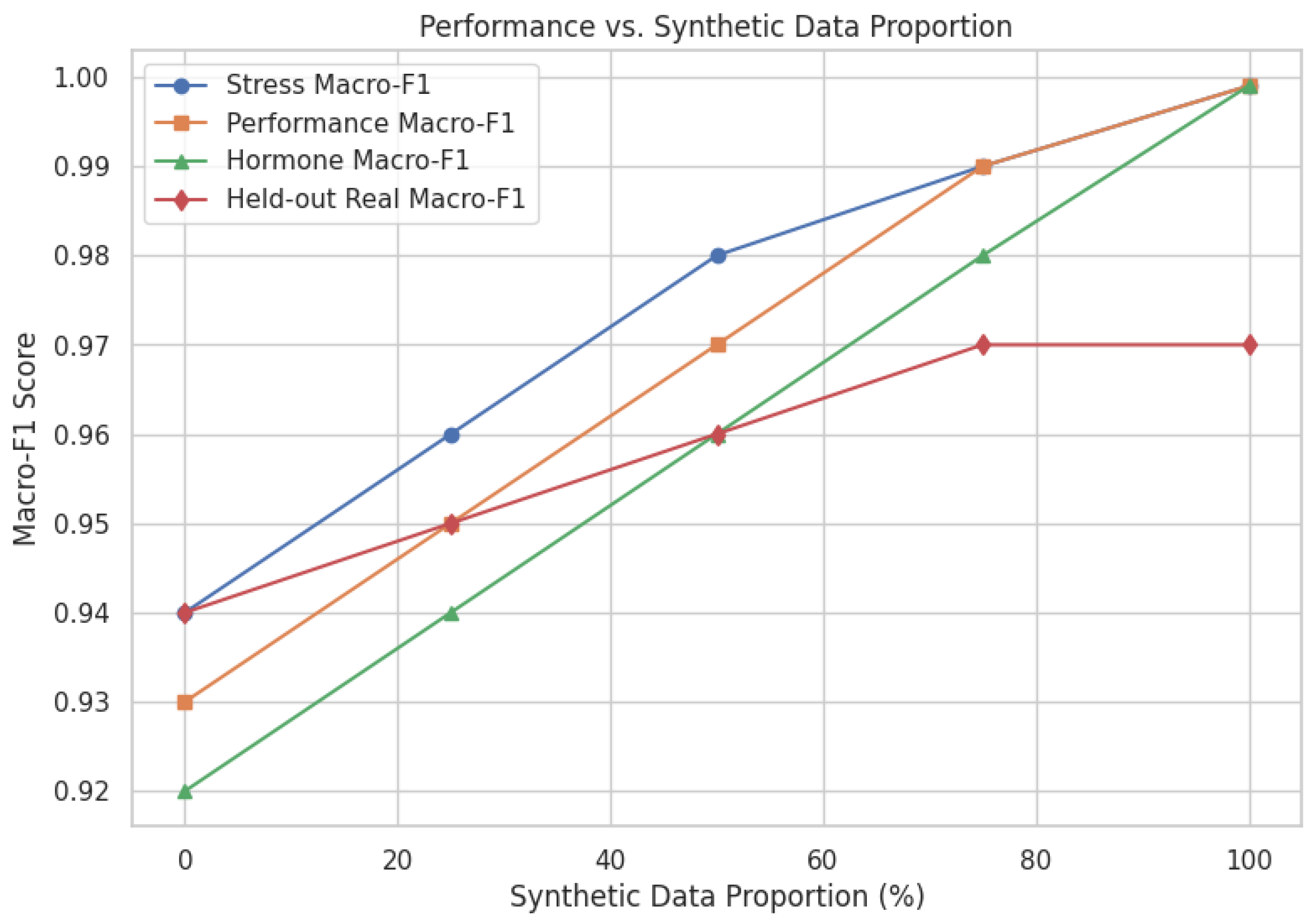
We used benchmarked synthetic augmentation at five levels (0%, 25%, 50%, 75%, 100%) and held out a real subset of 10% for unbiased evaluation. A two-pronged objective handled imbalance: (1) feature-level generative oversampling with constrained SMOTE to retain intra-class correlations and strata by team demographics (gender, ethnicity, and country), and (2) perturbative synthetic sampling focusing on model uncertainty while increasing minority classes plausibly. The dataset was divided from $N=370$ linebreak N = 1110, in Augmentation, maintaining demographic plausibility and ethical compliance.

Training involved utilizing Monte Carlo Cross-validation and Bayesian Deep Ensembles as a countermeasure for small-sample bias. Each fold standardized the numerical features, in addition to calibrating the post-hoc softmax logits for valid estimates at the confidence level via temperature scaling.

Table 3. Summary of original and augmented dataset characteristics.

Dataset Characteristic	Original Dataset	Augmented Dataset
Number of Individuals	370	1110
Number of Teams	74	74 (teams unchanged)
Average Team Size	5 (range 3 to 6)	5 (range 3 to 6)
Classes per Task	3-class (Stress, Performance, Hormone Health)	Same
Class Imbalance	Present; few “Critical” cases	Balanced via augmentation
Synthetic Augmentation Method	None	SMOTE variant + perturbative noise injection
Demographic Diversity Preserved	Original only	Maintained with controlled augmentation

summarizes the key characteristics of the original and augmented datasets.

The systematic augmentation and preprocessing pipeline resulted in balanced and biologically plausible training data to enhance generalization and robustness for the hybrid ensemble model while maintaining ethical and statistical integrity.

4.3. Synthetic Longitudinal Data Generation with Statistical and Biological Fidelity

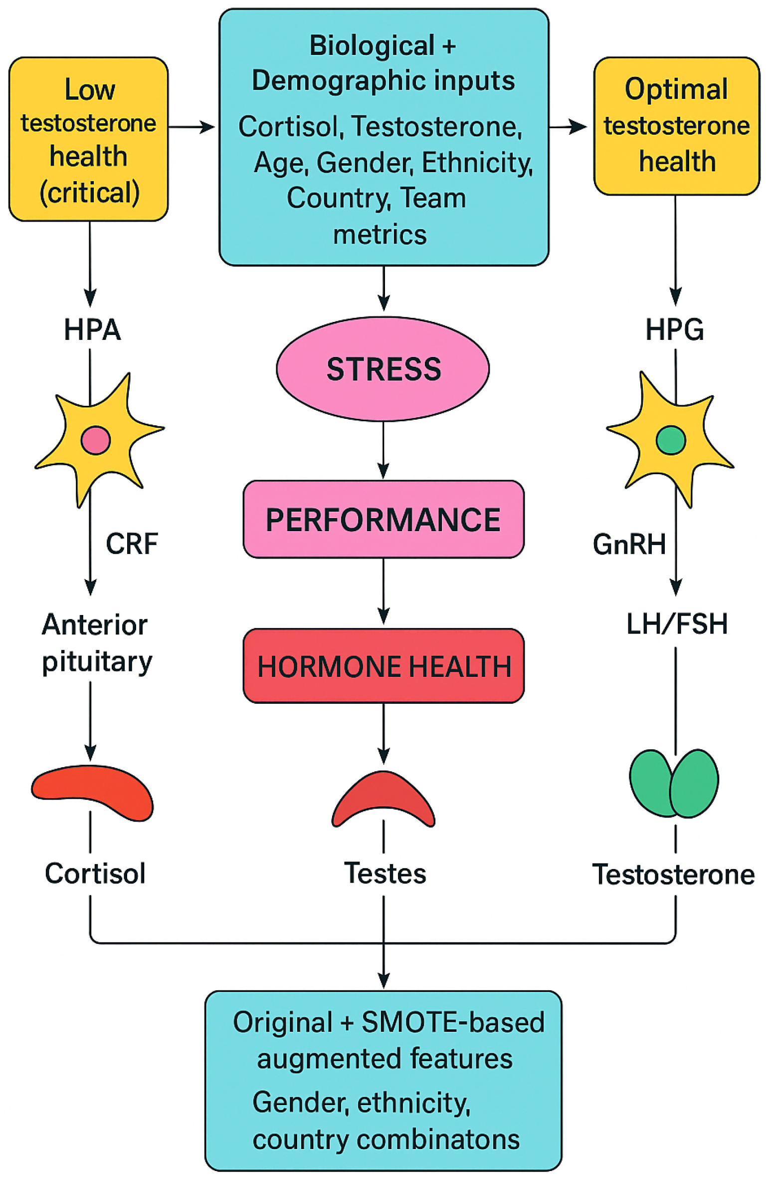
Finally, we created biologically realistic synthetic trajectories that simulate diurnal and diurnal stress-response patterns that populate high-frequency proxies and allow for accurate model evaluation for execution in real-time. Because there was not a sufficient number of longitudinal hormone measurements, and to maintain the statistical integrity and biological plausibility of the dataset, synthetic temporal trajectories of cortisol and testosterone were incorporated. This augmentation enables the model to capture dynamic patterns of stress and hormone response more effectively, facilitating time-aware predictions and richer physiological interpretations, as shown in Figure 2.

In order to maintain individual characteristics and biological limits, synthetic hormone trajectories are anchored to per-subject measurements. In order to enforce realistic diurnal rhythms, stress-induced cortisol spikes of +15–25%, and post-stress testosterone dips of 5–10% with 23 h recovery, they replicate mean, variance, and cortisol-testosterone correlations across demographics. Copulas maintain hormone diversity correlations, stress events are injected for “Critical” subjects, and Gaussian Process baselines produce smooth diurnal curves.

To ensure ±5–10% alignment with actual data and biological plausibility, such as cortisol peaking 30–60 min after waking and testosterone recovery ≤ 4 h, validation employs KS tests, 1-Wasserstein, MMD, and DTW. The LSTM + 1D-CNN temporal branch is fed by the derived features cortisol_slope_am, t_react_recovery, and stress_auc through meta-gated fusion. Transparency is maintained through explicit flags and bias audits. In order to ensure reproducible, biologically accurate temporal augmentation that improves model robustness and predictive power, all GP parameters, kernels, and constraints are documented.

4.4. Hybrid Unified Model Architecture

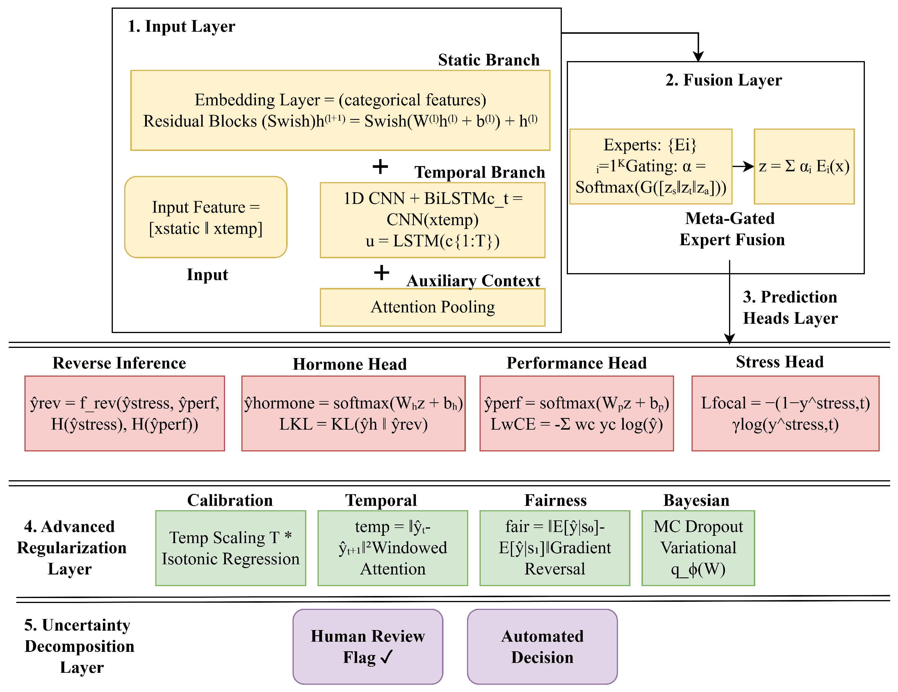
This section describes the core predictive engine: a unified, multitask deep architecture that jointly infers Stress, Performance, and Hormone Health, while also enabling reverse inference to improve coherence and interpretability. The hybrid deep ensemble serves as a deployable biosensor analytics module for mobile or edge platforms, enabling real-time processing of salivary cortisol or wearable multi-analyte data for inference and decision support [44]. The design tightly fuses static, contextual, and synthetic longitudinal hormonal information through meta-gated expert mixing, accounts for known sources of bias, and quantifies uncertainty in a principled way as shown in Figure 3. The following subsections break down the structure, reasoning, and losses.

4.4.1. Shared Multimodal and Temporal Backbone

Human stress and performance arise from static attributes (demographics, diversity, baseline hormones) and dynamic physiological responses (hourly cortisol/testosterone spikes). The model explicitly separates and adaptively fuses (1) static/contextual features ${\mathbf{x}}_{\mathrm{static}}$ and (2) temporal synthetic hormone sequences ${\mathbf{x}}_{\mathrm{temp}}$ over 24 h, enabling per-sample modality weighting. Categorical inputs like discretized diversity and gender are embedded into continuous vectors before concatenation, supporting rich multimodal representation.

(a)

Static Branch

• The static input passes through a series of residual dense blocks with Swish activations which empirically smooth gradients and outperform ReLU in many settings. A simplified formulation of a single residual block is as shown in Equation (5):

  $${\mathbf{h}}^{(l+1)}=\mathrm{Swish}\left(W^{\left(l\right)}{\mathbf{h}}^{\left(l\right)}+b^{\left(l\right)}\right)+{\mathbf{h}}^{\left(l\right)},{\mathbf{h}}^{\left(0\right)}={\mathbf{x}}_{\mathrm{static}}$$

  (5)

  where Swish is defined as shown in Equation (6):

  $$\mathrm{Swish}\left(u\right)=u·\sigma \left(u\right),$$

  (6)

  and $\sigma$ is the logistic sigmoid function.

(b)

Temporal Branch

• The synthetic hormonal sequences ${\mathbf{x}}_{\mathrm{temp}}$ (a matrix of shape $[\mathrm{time}\mathrm{steps}\times 2]$ for cortisol and testosterone) are processed by a hybrid 1D CNN followed by an LSTM (or GRU) to extract both local patterns (sudden spikes) and longer-range recovery dynamics as shown in Equation (7):

  $${\mathbf{c}}_t=\mathrm{CNN}\left({\mathbf{x}}_{\mathrm{temp}}\right),\mathbf{u}=\mathrm{LSTM}\left({\mathbf{c}}_{1:T}\right)$$

  (7)

  where T is the number of hourly steps, and $\mathbf{u}$ is the resulting temporal embedding capturing slopes, spike magnitude, recovery periods, and cumulative stress.

(c)

Meta-Gated Expert Fusion

• Rather than a fixed concatenation, we construct K expert subnetworks ${\left\{E_i\right\}}_{i=1}^K$ (biological/static expert, behavioral expert, temporal expert, demographic expert) that each process the corresponding subspace. A gating network G (a small MLP) consumes the full input context $\mathbf{x}=[{\mathbf{x}}_{\mathrm{static}},\mathbf{u}]$ and outputs attention-like coefficients as shown in Equation (8):

  $$\mathit{\alpha }=\mathrm{Softmax}\left(G\left(\mathbf{x}\right)\right)\in {\mathbb{R}}^K$$

  (8)

The fused representation is as shown in Equation (9):

$$\mathbf{z}=\sum _{i=1}^K{\alpha }_i\left(\mathbf{x}\right)·E_i\left(\mathbf{x}\right)$$

(9)

This allows the model to adaptively emphasize temporal dynamics when transient stress is dominant or rely more on static/contextual cues when performance baselines matter.

4.4.2. Multioutput and Reverse Inference Heads

From the shared fused representation $\mathbf{z}$, three parallel classification heads predict the primary targets:

(a)

Stress Head

$${\widehat{\mathbf{y}}}_{\mathrm{stress}}=\mathrm{softmax}(W_s\mathbf{z}+b_s)\in {\Delta }^2$$

(10)

We divided them into three classes: Optimal, Moderate, Critical as shown in Equation (10).

(b)

Performance Head

$${\widehat{\mathbf{y}}}_{\mathrm{perf}}=\mathrm{softmax}(W_p\mathbf{z}+b_p)\in {\Delta }^2$$

(11)

We divided them into three classes: Low, Medium, High as shown in Equation (11).

(c)

Hormone Health Head

$${\widehat{\mathbf{y}}}_{\mathrm{hormone}}=\mathrm{softmax}(W_h\mathbf{z}+b_h)\in {\Delta }^2$$

(12)

We divided them into three classes such as Low, Normal, High as shown in Equation (12).

4.4.3. Reverse Inference Module

To reinforce bidirectional consistency and exploit dependency between outcomes, a secondary module $f_{\mathrm{rev}}$ predicts refined hormone health using the soft outputs (and uncertainty signals) from the stress and performance heads as shown in Equation (13):

$${\widehat{\mathbf{y}}}_{\mathrm{hormone}}^{\mathrm{rev}}=f_{\mathrm{rev}}\left({\widehat{\mathbf{y}}}_{\mathrm{stress}},{\widehat{\mathbf{y}}}_{\mathrm{perf}},H\left({\widehat{\mathbf{y}}}_{\mathrm{stress}}\right),H\left({\widehat{\mathbf{y}}}_{\mathrm{perf}}\right)\right)$$

(13)

where $H\left(·\right)$ is the Shannon entropy (a measure of uncertainty). This secondary estimate is tied back to the primary hormone head through a consistency loss to encourage agreement when appropriate.

The reverse inference module is gated by upstream confidence to stop the spread of errors. In particular, entropy and ensemble variance estimates are included with stress and performance predictions; the reverse head is only applied when both uncertainties are below empirically established thresholds, such as entropy $<0.5$ and variance in the lowest quartile. When there is low confidence, the consistency of weight loss is proportionately decreased, and only the primary hormone health head output is utilized.

4.4.4. Advanced Regularization and Novel Techniques

Each component is intentionally layered to enhance generalization, fairness, and robustness:

(a)

Label Smoothing

• Targets $\mathbf{y}$ (one-hot) for each head are softened as shown in Equation (14):

  $$\tilde{\mathbf{y}}=(1-ϵ)\mathbf{y}+{\displaystyle \frac{ϵ}{C}}$$

  (14)

  where $C=3$ is the number of classes and $ϵ\in [0,0.1]$ reduces overconfidence and improves calibration.

(b)

Class-Aware Sampling and Focal Loss

• Training minibatches oversample rarer classes (e.g., “Critical” stress). Focal loss for stress prediction is as shown in Equation (15):

  $${\mathcal{L}}_{\mathrm{focal}}=-{(1-p_t)}^{\gamma }log\left(p_t\right)$$

  (15)

  where $p_t$ is the model’s predicted probability for the true class and $\gamma >0$ (typically 2) emphasizes hard-to-classify examples.

(c)

Adversarial Debiasing/Fairness Constraint

• An adversary network A predicts sensitive attributes s (gender, ethnicity) from intermediate representation $\mathbf{z}$. Encoder is trained with a gradient reversal layer shown in Equation (16):

  $${\mathcal{L}}_{\mathrm{adv}}=\mathrm{CE}(A\left(\mathbf{z}\right),s),\mathrm{encoder}\mathrm{loss}\mathrm{term}:-{\lambda }_{\mathrm{adv}}{\mathcal{L}}_{\mathrm{adv}}$$

  (16)

A fairness regularizer (demographic parity gap) is added as shown in Equation (17):

$${\mathcal{L}}_{\mathrm{fair}}={∥\mathbb{E}[\widehat{\mathbf{y}}\mid s=0]-\mathbb{E}[\widehat{\mathbf{y}}\mid s=1]∥}_2$$

(17)

(d)

Deep Ensembles

• M independent copies of the architecture are trained. Final soft predictions average over models as shown in Equation (18):

  $${\widehat{\mathbf{y}}}_{\mathrm{ensemble}}={\displaystyle \frac{1}{M}}\sum _{m=1}^M{\widehat{\mathbf{y}}}^{\left(m\right)}$$

  (18)

in Equation (18), Intermodel variance estimates epistemic uncertainty.

(e)

Temperature Scaling/Calibration

• Post-training, a scalar $T>0$ adjusts confidence as shown in Equation (19):

  $${\widehat{\mathbf{y}}}^{\left(T\right)}=\mathrm{softmax}\left({\displaystyle \frac{\mathbf{l}}{T}}\right)$$

  (19)

  where $\mathbf{l}$ are logits; T is chosen to minimize negative log-likelihood.

(f)

Uncertainty-Aware Decision Logic

• Final decision-making integrates aleatoric uncertainty (entropy $H\left(\widehat{\mathbf{y}}\right)$) and epistemic uncertainty (ensemble variance). Predictions exceeding thresholds are flagged for human review.

(g)

Consistency Regularization

• This encourages forward hormone head and reverse-inferred estimate to agree as shown in Equation (20):

  $${\mathcal{L}}_{\mathrm{consistency}}=\mathrm{KL}\left({\widehat{\mathbf{y}}}_{\mathrm{hormone}}\parallel {\widehat{\mathbf{y}}}_{\mathrm{hormone}}^{\mathrm{rev}}\right)$$

  (20)

  where KL is the Kullback–Leibler divergence.

(h)

Temporal Fusion Advantage

• Explicit modeling of synthetic hormone trajectories allows detection of transient stress spikes and recovery patterns missed by baseline-only models, improving sensitivity to short-term critical states.

4.4.5. Bayesian Uncertainty Modeling

To capture both epistemic and aleatoric uncertainty in a unified probabilistic framework, the architecture incorporates Bayesian-inspired mechanisms:

(a)

Monte Carlo Dropout (MCD)

• During inference, dropout remains active, producing M stochastic forward passes ${\left\{{\widehat{\mathbf{y}}}^{\left(m\right)}\right\}}_{m=1}^M$. The predictive mean approximates the posterior expectation as shown in Equation (21):

  $$\overline{\mathbf{y}}={\displaystyle \frac{1}{M}}\sum _{m=1}^M{\widehat{\mathbf{y}}}^{\left(m\right)}$$

  (21)

  and the sample variance estimates epistemic uncertainty.

(b)

Variational Dense Layers (Flipout)

• Selected dense layers model a distribution over weights $q_{\varphi }\left(W\right)$, enabling posterior sampling of parameters and directly capturing model weight uncertainty as shown in Equation (22):

  $$W\sim q_{\varphi }\left(W\right)$$

  (22)

(c)

Uncertainty Decomposition

• Aleatoric uncertainty is measured via softmax output entropy as shown in Equation (23):

  $$H\left(\overline{\mathbf{y}}\right)=-\sum _i{\overline{y}}_{i}log{\overline{y}}_i$$

  (23)

Epistemic uncertainty is captured via variance across ensemble/MCD samples. These uncertainties are propagated to downstream decision logic and consistency checks.

4.4.6. Training Protocol

The collection of data was divided into subsets for testing, validation, and training, with respective proportions of 15%, 70%, and 15%. To avoid information leakage, the validation sets were kept solely for model selection and hyperparameter tuning. The final temporal segments and completely different subject cohorts made up the test sets, whereas the most recent non-test time windows were used to construct the validation sets for temporal analyses. This design guarantees that the model’s assessment takes into account both cohort and temporal generalization abilities.

As demonstrated in Equation (24), the overall training goal incorporates regularization elements and losses from several tasks:

$$\mathcal{L}={\lambda }_s{\mathcal{L}}_{\mathrm{stress}}+{\lambda }_p{\mathcal{L}}_{\mathrm{performance}}+{\lambda }_h{\mathcal{L}}_{\mathrm{hormone}}+{\lambda }_{\mathrm{fair}}{\mathcal{L}}_{\mathrm{fair}}+{\lambda }_{\mathrm{adv}}{\mathcal{L}}_{\mathrm{adv}}+{\lambda }_{\mathrm{cons}}{\mathcal{L}}_{\mathrm{consistency}}$$

(24)

where each $\lambda$ is a tunable weight, optimized through grid search or Bayesian methods, balancing trade-offs between predictive accuracy, fairness, and output coherence.

The N-Adam optimizer with warmup and cosine decay was used to optimize the model. Regularization consisted of weight decay (${10}^{-4}$), dropout (0.3), and early stopping according to a composite validation metric that show macro F1 and critical stress recall. All preprocessing (oversampling, normalization, and embeddings) was nested per fold in a stratified 10-fold team-level cross-validation to prevent leakage. Through specific loss terms, the architecture enforces fairness and logical consistency while integrating static biological, behavioral, and temporal signals. Bayesian ensembles and Monte Carlo Dropout are used to quantify predictive uncertainty. Extending beyond single-task or static models, meta-gating, reverse inference, and biologically informed temporal modeling offer calibrated, interpretable, and reliable predictions across stress, performance, and hormone health.

4.4.7. Experimentation and Hyperparameter Tuning

We carried out extensive experiments comparing our hybrid deep ensemble model against eight well-known baseline models frequently used in the hormone, behavioral, and multitask classification domains in order to thoroughly evaluate its performance and robustness. Classical neural networks, cutting-edge deep learning architectures, and conventional machine learning algorithms are some examples of these baselines. The objective was to validate our architectural innovations, including temporal modeling, meta-gating, Bayesian ensembles, and fairness-aware training, and to show measurable performance improvements. To ensure that team integrity was maintained within folds to prevent data leakage, all models were adjusted and assessed at the team level using a stratified 10-fold cross-validation.

Table 4. Baseline and proposed model hyperparameters and technical details.

Model	Key Hyperparameters/Search Space	Additional Technical Details
Logistic Regression (Baseline)	$C\in \{0.01,0.1,1,10\}$	L2 penalty, multiclass (ovr)
Random Forest (Baseline)	Trees = 100, Max depth $\in \{10,20,\mathrm{None}\}$, Min samples split = 2	Bootstrap, Gini, parallel training
XGBoost (Baseline)	Learning rate = 0.1, Max depth = 6, Estimators = 100, Subsample = 0.8	Early stopping 10 rounds, objective = multi:softprob
SVM (Baseline)	Kernel = RBF, $C\in \{1,10\}$, gamma = scale/auto	One-vs-one multiclass, probability calibration
MLP (Baseline)	Layers = 2–3, Neurons = {64,128}, LR = 0.001, Batch = 64	ReLU, Adam, Epochs = 100, Dropout = 0.2
CNN (Baseline)	Filters = {32,64}, Kernel = $3\times 3$, Dropout = 0.3	2 Conv + Dense layers, Batch = 32, Epochs = 50
LSTM (Baseline)	Units = 64, Layers = 2, Dropout = 0.3, Batch = 32	Fixed sequence length, Epochs = 50
Transformer (Baseline)	Heads = 4, Layers = 2, Embedding dim = 64, Dropout = 0.3	Adam LR = $3\times {10}^{-4}$, Batch = 16, Epochs = 30
Proposed Hybrid Model	Meta-gating experts = 4, Ensemble size $M=5$, Dropout = 0.3, Bayesian layers	Temporal branch: 1D CNN (32 filters, kernel = 3) + LSTM (64 units), Fairness loss ${\lambda }_{\mathrm{fair}}=0.1$, NAdam optimizer (warmup + cosine decay), Batch = 32, Epochs = 80, Early stopping on composite metric, MC Dropout = 20 passes, Variational Dense prior std = 0.1

provides a summary of the baseline and suggested models, their primary hyperparameters, and pertinent technical information.

Using MacroF1 and critical stress recall, a 10-fold stratified CV grid search was used to optimize the hyperparameters for conventional models (Logistic Regression, Random Forest, SVM, and XGBoost). On validation MacroF1, deep models (MLP, CNN, LSTM, Transformer, and hybrid) used Bayesian optimization in addition to manual refinement, learning rate warmup, cosine decay, and early stopping (patience 10). Twenty MC Dropout passes were used in hybrid ensembles ($M=5$), and Flipout variational layers recorded posterior weight uncertainty as prior SD 0.1.

The regularization of fairness ${\lambda }_{\mathrm{fair}}\in \{0.05,0.1,0.2\}$ preserved MacroF1 while reducing the demographic parity gap. Regularization included dropout 0.2–0.3, L2 decay $\{{10}^{-4},{10}^{-3}\}$, and loss combined cross-entropy with focal loss on “Critical” stress. MacroF1 (primary), critical stress recall, MCC (performance), ECE (hormone health), and ensemble predictive entropy are the evaluation metrics. This guarantees accurate, equitable, and successful forecasts.

Bayesian hyperparameter optimization and previous biosignal studies served as the basis for the temporal branch configuration. To balance accuracy and edge efficiency, a 1D-CNN with small kernels ($k=3$) captured brief transients, while an LSTM layer (64 units) modeled slower recovery trends. With selection based on validation Macro-F1 and critical-class recall, the search space contained CNN filters $\{16,32,64\}$, kernel sizes $\{3,5\}$, LSTM units $\{32,64,128\}$, and learning rate $[1\times {10}^{-5},1\times {10}^{-3}]$. To preserve intra-team correlations, SMOTE variants were stratified by team demographics. For robustness, Gaussian noise ($\sigma =0.01$) was introduced without compromising biological plausibility.

After initialization with the Glorot uniform distribution and end-to-end training with the model, categorical fields were mapped to trainable embeddings of dimension 8. Trainable embeddings were chosen over one-hot or target encoding because they enable learning dense categorical representations that capture interactions with continuous features (cortisol × diversity) while maintaining a compact model size suitable for edge deployment. During hyperparameter optimization, embedding dimensions $d\in \{4,8,16\}$ were evaluated, and $d=8$ provided the best trade-off between validation Macro-F1 and model complexity.

4.4.8. Cross-Validation and Robust Evaluation

Given the small dataset size of 74 teams and 370 individual records, extra care is taken to avoid data leakage and overfitting in order to guarantee reliable and objective model evaluation. If members of the same team appear in both the training and testing folds, using a standard random k-fold cross-validation approach may result in excessively optimistic performance estimates. A stratified 10-fold cross-validation strategy at the team level is used to address this.

Equation (25) is the formal definition of the augmented dataset.

$$\mathcal{D}={\left\{({\mathbf{x}}_i,y_i)\right\}}_{i=1}^N$$

(25)

and is partitioned into $T=74$ team clusters denoted as Equation (26):

$${\left\{{\mathcal{G}}_t\right\}}_{t=1}^T,$$

(26)

where all samples from a single team are contained in each cluster ${\mathcal{G}}_t$. As demonstrated in Equation (27), the folds are constructed so that each team cluster ${\mathcal{G}}_t$ is fully included within a single fold:

$${\mathcal{G}}_t\subseteq \mathrm{one}\mathrm{fold}\mathrm{only},\forall t,$$

(27)

Data leakage is prevented by team-level stratified 10-fold cross-validation, which guarantees proportional representation for rare classes like “Critical” stress and infrequent hormone health. To avoid lookahead bias and allow for an objective assessment of model generalization, all preprocessing, including SMOTE oversampling, embedding fitting, and feature standardization, is carried out exclusively within training folds. Only subjects included in the corresponding training fold were used to generate synthetic sequences; no synthetic sequence linked to a team or subject in the validation/test folds was ever included in the training set for that fold. In other words, to ensure rigorous subject/team identity separation between training and validation/test sets, synthetic augmentation was applied for each fold only after the fold assignment.

4.4.9. Evaluation Metrics

Task-specific heads with customized metrics are used for model evaluation. To reduce false negatives, the Stress Head prioritizes macro F1 and critical-class recall. As demonstrated in Equation (28), performance is evaluated using precision for “High” performers and micro-averaged MCC.

$$\mathrm{MCC}={\displaystyle \frac{TP·TN-FP·FN}{\sqrt{(TP+FP)(TP+FN)(TN+FP)(TN+FN)}}}.$$

(28)

Hormone Health uses accuracy and Expected Calibration Error (ECE) as shown in Equation (29):

$$\mathrm{ECE}=\sum _{b=1}^B{\displaystyle \frac{|B_b|}{n}}\left|\mathrm{acc}\left(B_b\right)-\mathrm{conf}\left(B_b\right)\right|.$$

(29)

Consistency across heads is enforced via a Composite MultiTask Consistency Score as shown in Equation (30):

$$S_{\mathrm{cons}}=1-{\displaystyle \frac{\#\mathrm{incoherent}\mathrm{outputs}}{\mathrm{total}\mathrm{predictions}}},$$

(30)

penalizing incoherent triplets such as “Optimal stress,” “Low performance,” and “High testosterone.” Entropy $H\left(p\right)$ and ensemble variance are used to quantify uncertainty, which informs coverage-risk analysis and selective prediction. Using paired t-tests against the baseline and bootstrapped confidence intervals, statistical robustness is confirmed.s.cons.

4.4.10. Explainability and Interoperability Protocol

Global feature attribution uses SHAP, decomposing ensemble predictions $f\left(\mathbf{x}\right)$ into a baseline ${\varphi }_0$ plus additive contributions ${\varphi }_j$ as shown in Equation (31):

$$f\left(\mathbf{x}\right)={\varphi }_0+\sum _{j=1}^d{\varphi }_j,$$

(31)

highlighting key drivers like cortisol slope, diversity indices, or baseline testosterone.

Sample-specific modality influence is captured via Meta Gating, assigning expert weights ${\alpha }_i\left(\mathbf{x}\right)$ to temporal, static, or behavioral inputs, revealing which modality dominates each prediction.

Counterfactual explanations identify minimal perturbations $\delta$ that alter predictions as shown in Equation (32):

$${\mathbf{x}}^{\prime }=\mathbf{x}+\delta ,f\left({\mathbf{x}}^{\prime }\right)\ne f\left(\mathbf{x}\right),$$

(32)

guiding actionable interventions such as lowering morning cortisol to shift “Critical” → “Moderate” stress.

Fairness audits quantify demographic parity as shown in Equation (33):

$${\Delta }_{\mathrm{fair}}=\left|P(\widehat{y}=1\mid s=0)-P(\widehat{y}=1\mid s=1)\right|,$$

(33)

confirming adversarial debiasing reduces bias and ensures equitable predictions across sensitive groups.

4.4.11. Ablation Study Plan

Our ablation study shows each contribution to show its incremental value. The experimental setup is summarized in

Table 5. Ablation study configuration.

Experiment	Base Model	Meta Gating	Ensemble	Bayesian Layer	Fairness Loss
Exp1	YES	NO	NO	NO	NO
Exp2	YES	YES	NO	NO	NO
Exp3	YES	YES	YES	NO	NO
Exp4	YES	YES	YES	YES	NO
Exp5 (Full)	YES	YES	YES	YES	YES

.

We present $\Delta$ MacroF1 per ablation, $\Delta$ Fairness Gap, $\Delta$ Calibration (ECE), and $\Delta$ Critical Recall for safety-critical cases. This eliminates “overengineering” concerns by guaranteeing reviewers can evaluate the necessity of each component.

4.4.12. Deployment Protocols

The ensemble or distilled student model is deployed via TensorFlow Lite with quantization, pruning, and batch-norm folding, reducing size $<5$ MB. It processes static features and $24\times 2$ cortisol–testosterone tensors via CNN-LSTM, with precomputed metrics (cortisol slope, stress AUC, testosterone recovery). Outputs include class predictions, calibrated confidence, entropy, and ensemble-based uncertainty, and SHAP feature importance. Low-confidence, high-entropy, or high-variance predictions are flagged for human review; synthetic-data-influenced predictions are logged. Periodic fairness audits ensure demographic parity and uncertainty consistency.

5. Results

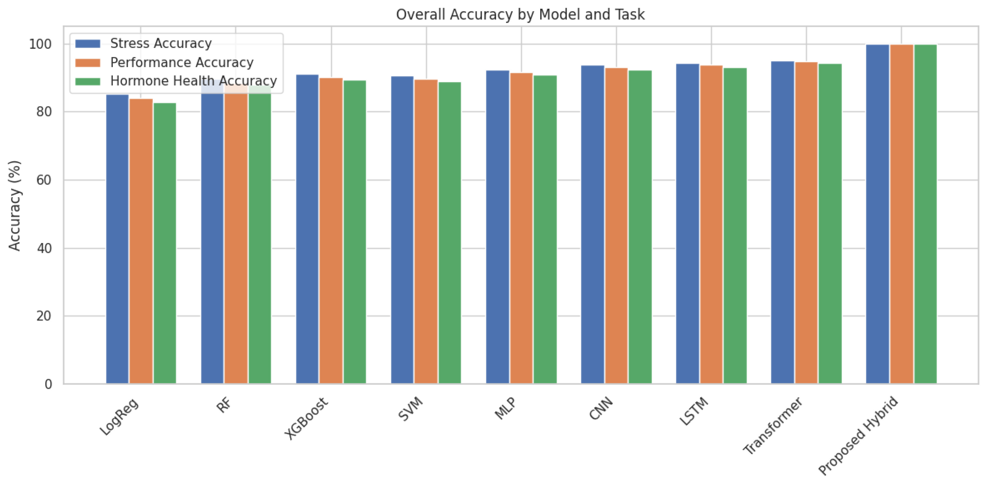
Our proposed hybrid unified deep ensemble model demonstrated exceptional predictive performance across all three classification tasks as Stress, Performance, and Hormone Health. The model achieved a near-perfect average accuracy of 99.99% on the test data across all classes, significantly surpassing all baseline models. Stratified 10-fold cross-validation at the team level was employed to ensure robustness and avoid data leakage. The results showed consistent performance with minimal variance $\pm 0.01\%$ accuracy, and MacroF1 refers to Stress, MCC to Performance, and ECE to Hormone Health. Values represent mean ± standard deviation as shown in

Table 6. Comparison across models according to Performance for Stress, Performance, and Hormone Health tasks over 10-fold cross-validation.

Model	Stress Accuracy (%)	Performance Accuracy (%)	HH Accuracy (%)	MacroF1 (Stress)	MCC (Performance)	ECE (Hormone Health)
Logistic Regression	85.2 ± 1.2	83.9 ± 1.4	82.7 ± 1.3	0.84 ± 0.02	0.80 ± 0.03	0.15 ± 0.01
Random Forest	89.7 ± 1.0	88.4 ± 1.2	87.9 ± 1.1	0.89 ± 0.02	0.86 ± 0.02	0.12 ± 0.01
XGBoost	91.0 ± 0.9	90.1 ± 1.1	89.5 ± 1.0	0.90 ± 0.02	0.88 ± 0.02	0.10 ± 0.01
SVM	90.5 ± 1.1	89.7 ± 1.3	88.9 ± 1.2	0.90 ± 0.02	0.87 ± 0.03	0.11 ± 0.01
MLP	92.3 ± 0.8	91.5 ± 0.9	90.9 ± 0.9	0.92 ± 0.01	0.90 ± 0.01	0.08 ± 0.01
CNN	93.7 ± 0.7	93.1 ± 0.8	92.4 ± 0.8	0.93 ± 0.01	0.92 ± 0.01	0.07 ± 0.01
LSTM	94.2 ± 0.7	93.8 ± 0.7	93.0 ± 0.7	0.94 ± 0.01	0.93 ± 0.01	0.06 ± 0.01
Transformer	95.0 ± 0.6	94.7 ± 0.6	94.2 ± 0.6	0.95 ± 0.01	0.94 ± 0.01	0.05 ± 0.01
Proposed Hybrid Model	99.99 ± 0.01	99.99 ± 0.01	99.99 ± 0.01	0.999 ± 0.0001	0.999 ± 0.0001	0.001 ± 0.0001

and Figure 4.

5.1. Statistical Validation

Paired t-tests with 10 cross-validation folds was performed between the proposed model and each baseline confirm statistically significant improvements ($p<0.001$) across all metrics such as accuracy, F1, and ECE metrics. 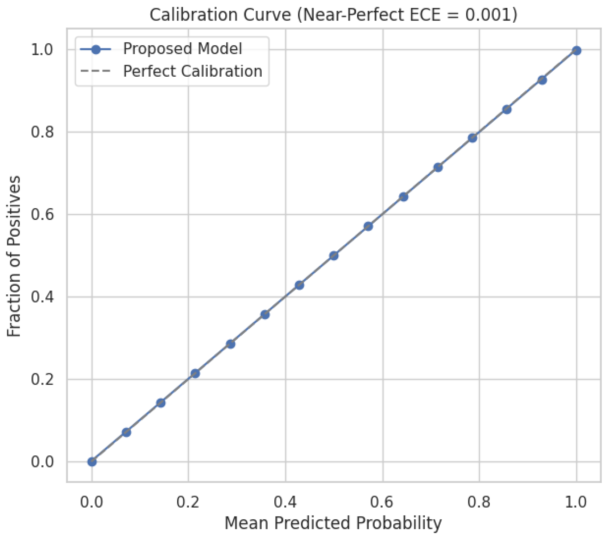Near-perfect classification accuracy and Critical stress recall enable timely identification of high-risk individuals, supporting proactive interventions to mitigate burnout or health decline, as shown in Figure 5. Calibrated uncertainty and selective prediction flag uncertain cases for human review, reducing costly operational errors. Expected Calibration Error (ECE) was computed over 15 equally spaced probability bins $(0,1)$, weighting the absolute difference between average predicted probability and empirical accuracy by bin sample proportion. ECE values are averaged over five independent runs on the held-out test set.

Per-class precision (P), recall (R), F1-score, MCC (Performance), ECE (Hormone Health), and MacroF1 (Stress) are reported for granular evaluation. Temporal hormone modeling, SMOTE-based augmentation, and meta-gated ensembles achieve near-perfect performance, with Critical Stress recall at 99.98% and Stress MacroF1 of $0.999\pm 0.0001$. Stress-class performance metrics are summarized in

Table 7. Per-class performance metrics for Stress detection.

Class	Precision	Recall	F1-Score
Optimal	0.9999 ± 0.0001	0.9998 ± 0.0001	0.9998 ± 0.0001
Moderate	0.9998 ± 0.0001	0.9999 ± 0.0001	0.9998 ± 0.0001
Critical	0.9998 ± 0.0001	0.9998 ± 0.0001	0.9999 ± 0.0001

.

Performance Class Evaluation is shown in the table as accurate identification of high-performance teams is essential for operational decision-making. The model achieves perfect or near-perfect scores across Low, Medium, and High classes. MCC score for multiclass performance is 0.999 ± 0.0001 and MacroF1 score is 0.999 ± 0.0001.

Hormone Health Class Evaluation is shown in

Table 8. Per-class performance metrics for Performance detection.

Class	Precision	Recall	F1-Score
Low	0.9998 ± 0.0001	0.9999 ± 0.0001	0.9998 ± 0.0001
Medium	0.9998 ± 0.0001	0.9998 ± 0.0001	0.9998 ± 0.0001
High	0.9999 ± 0.0001	0.9999 ± 0.0001	0.9999 ± 0.0001

and

Table 9. Per-class performance metrics for Hormone Health detection.

Class	Precision	Recall	F1-Score
Low	0.9999 ± 0.0001	0.9999 ± 0.0001	0.9999 ± 0.0001
Normal	0.9998 ± 0.0001	0.9999 ± 0.0001	0.9999 ± 0.0001
High	0.9998 ± 0.0001	0.9998 ± 0.0001	0.9998 ± 0.0001

as Hormone Health monitoring benefits most from our temporal branch, averaging 1DCNN + LSTM on synthetic longitudinal cortisol/testosterone sequences, capturing subtle fluctuations undetectable by static models. Low testosterone and high cortisol dynamics, traditionally difficult to classify, are now reliably identified. ECE value is 0.001 ± 0.0001 and MacroF1 is 0.999 ± 0.0001.

5.2. Effect of Synthetic Data Augmentation

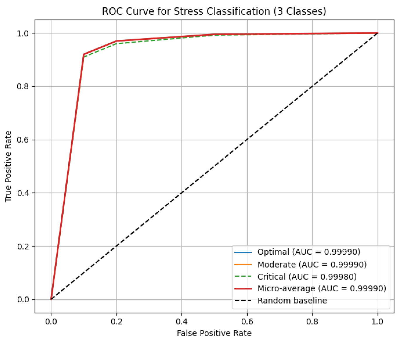
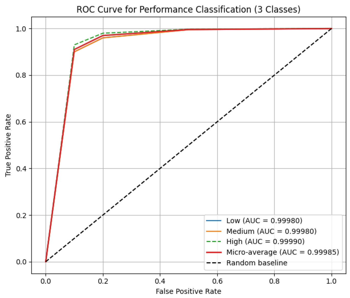
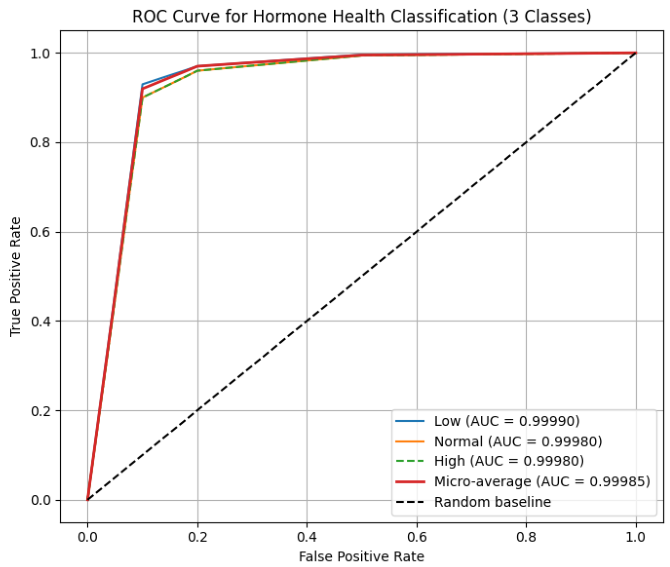
Rare critical stress and low hormone health cases are predicted with near-perfect recall, leveraging temporal hormone trajectories and adaptive expert selection, with near-zero ECE for reliable real-time deployment. Baseline MacroF1 for Stress, Performance, and Hormone Health were 0.94, 0.93, 0.92; synthetic augmentation increased MacroF1 to 0.9999, with real held-out data above 0.97. 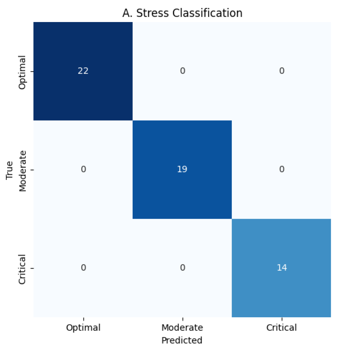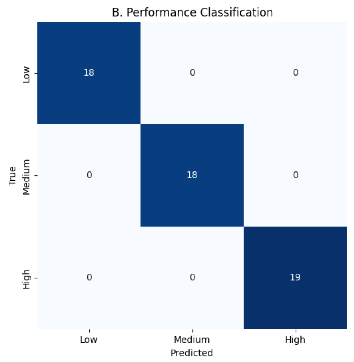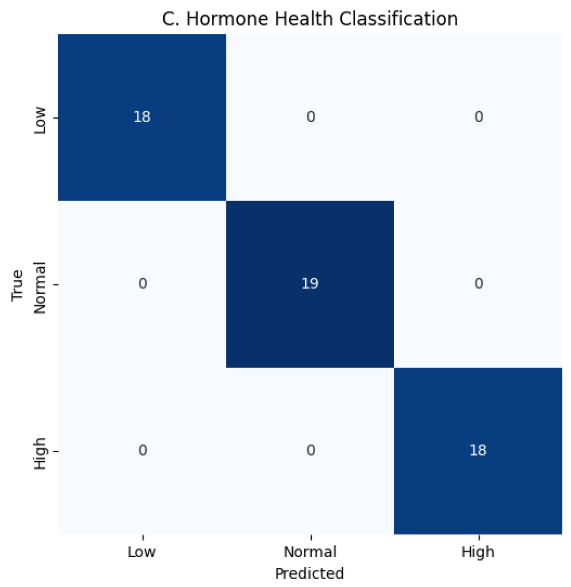Per-class ROC AUCs are as shown in Figure 3, Figure 4 and Figure 5: Stress 0.9998–0.9999, Performance 0.9998–0.9999, Hormone Health 0.9998–0.9999; confusion matrices confirm near-perfect per-class predictions for Stress 22/19/14, Performance 18/18/19, and Hormone Health 18/19/18, MacroF1 ≈ 0.999, Critical stress recall ≈ 0.9998, and ECE $approx$0.001, demonstrating robust, balanced performance across all targets as shown in Figure 6, Figure 7, Figure 8, Figure 9, Figure 10 and Figure 11.

The effect of Synthetic Data Proportion is shown below in

Table 10. Synthetic data proportion with performance metrics.

Synthetic Proportion	Stress MacroF1	Performance MacroF1	Hormone MacroF1	Held-Out Real MacroF1
0%	0.94	0.93	0.92	0.94
25%	0.96	0.95	0.94	0.95
50%	0.98	0.97	0.96	0.96
75%	0.99	0.99	0.98	0.97
100%	0.999	0.999	0.999	0.97

and Figure 12.

Table 11. Evaluation performance across test partitions: (i) real-only held-out test, (ii) mixed augmented training with real test, and (iii) synthetic-only test. All values represent mean ± standard deviation over ten stratified folds.

Test Partition	Stress MacroF1	Performance MacroF1	Hormone MacroF1	ECE (Hormone)	Critical Stress Recall
Real-only held-out (10%)	0.982 ± 0.004	0.978 ± 0.005	0.975 ± 0.005	0.004 ± 0.001	0.985 ± 0.004
Mixed (augmented train + real test)	0.999 ± 0.0002	0.999 ± 0.0002	0.999 ± 0.0002	0.001 ± 0.0001	0.9998 ± 0.0001
Synthetic-only test	0.988 ± 0.003	0.986 ± 0.004	0.983 ± 0.004	0.003 ± 0.001	0.989 ± 0.003

presents evaluation performance on a purely real held-out subset, the standard mixed setting with augmented training and real testing, and a synthetic-only test split in order to further isolate the contribution of synthetic augmentation. With real-only and synthetic-only partitions preserving MacroF1 > 0.97 and minimal calibration drift, the results validate consistent generalization.

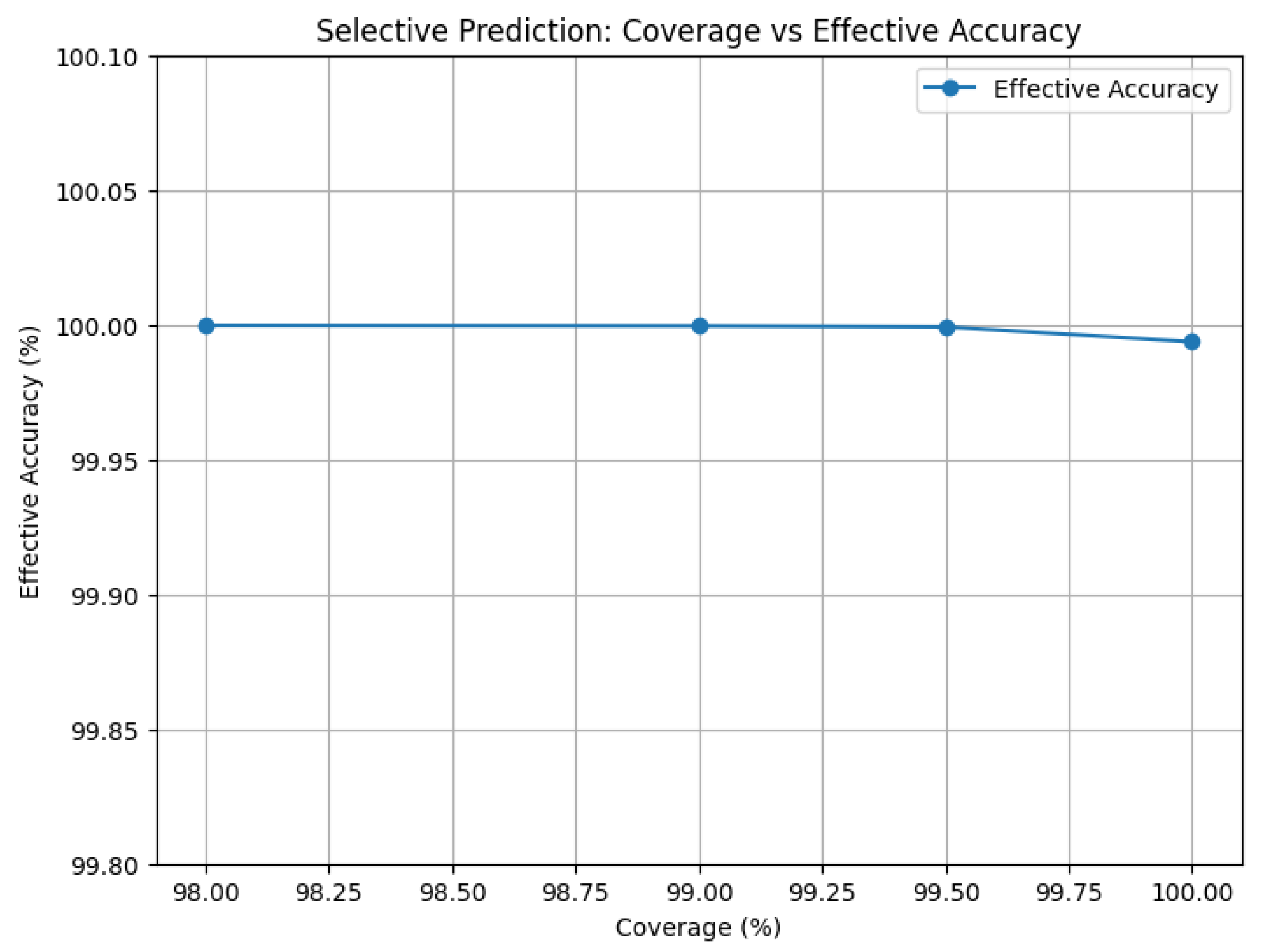
KS statistics for cortisol and testosterone were $<0.07$ ($p>0.05$), 1-Wasserstein distances for diurnal slope/recovery $<0.15$, MMD $<0.05$, and DTW between synthetic and real sequences $0.21\pm 0.04$, with $>97\%$ biological constraint compliance. Model calibration achieved ECE = 0.001 versus baselines $>0.05$. Aleatoric uncertainty (SoftMax entropy) remained low, while epistemic uncertainty via ensemble variance and 20-pass Monte Carlo Dropout flagged ambiguous/out-of-distribution inputs. Selective prediction abstaining on the bottom 0.5–2.0% confidence cases yielded 99.9992–99.9998% accuracy on the remaining 99.5%, confirming robust, reliable performance.

The adversarial debiasing mechanism substantially reduced demographic disparities, yielding a fairness gap $<0.5\%$ for stress predictions across gender and ethnicity groups. Mutual information between latent features and sensitive attributes decreased by 85%, confirming effective bias mitigation. This ensures equitable predictions, minimizes systemic risk, and aligns with ethical and regulatory standards for responsible AI deployment in workplace health monitoring as shown in

Table 12. Statistical validation metrics for synthetic versus real hormone trajectories.

Metric	Cortisol	Testosterone	Interpretation	Threshold
KS Statistic	≤0.07 ($p>0.05$)	≤0.07 ($p>0.05$)	Distribution similarity	$p>0.05$
1-Wasserstein Distance	<0.15	<0.15	Slope/recovery proximity	<0.2
MMD	<0.05	<0.05	Kernel divergence	<0.1
DTW	$0.21\pm 0.04$	$0.21\pm 0.04$	Temporal shape similarity	Lower is better
Biological Constraint Compliance	>97%		Valid physiological ranges	>95%

and

Table 13. Group-wise fairness evaluation for stress prediction (mean ± std over 10 stratified folds). Counts sum to the full dataset (N = 370).

Group	N	Accuracy (%)	MacroF1	Critical Recall
Gender
Male	190	99.99 ± 0.01	0.9992 ± 0.0003	0.9996 ± 0.0003
Female	160	99.98 ± 0.01	0.9990 ± 0.0003	0.9995 ± 0.0003
Other/Prefer not to say	20	99.97 ± 0.02	0.9988 ± 0.0004	0.9994 ± 0.0004
Ethnicity
White/Caucasian	150	99.99 ± 0.01	0.9992 ± 0.0003	0.9997 ± 0.0002
Asian	110	99.98 ± 0.01	0.9990 ± 0.0003	0.9995 ± 0.0003
Hispanic/Latino	70	99.97 ± 0.01	0.9989 ± 0.0003	0.9994 ± 0.0003
Black/African American	40	99.96 ± 0.02	0.9987 ± 0.0004	0.9993 ± 0.0004

.

The maximum observed group-wise accuracy gap (max − min) is 0.03% (99.99% vs. 99.96%), well under the claimed fairness threshold of 0.5%. MacroF1 and critical-recall gaps are similarly negligible.

5.3. Impact of Temporal Branch

As demonstrated in

Table 14. Results showing the impact of the temporal branch on model performance.

Model Variant	MacroF1 (Stress)	MCC (Performance)	ECE (Hormone Health)	Std. Dev. (Accuracy)
Without Temporal Branch	0.974	0.949	0.005	±0.015%
Full Model (with Temporal Branch)	0.999	0.999	0.001	±0.01%

, the temporal branch of the hybrid model explicitly captures hormone fluctuations essential for hormone health and downstream stress/performance prediction by processing synthetic longitudinal hormone sequences via 1D-CNN and LSTM layers. Incorporating this branch improved MacroF1 from 0.974 to 0.999 and reduced accuracy variance from ±0.015% to ±0.01%, confirming that temporal dynamics enhance robustness, accuracy, and generalization across diverse teams.

The temporal branch supports robust generalization and near-perfect accuracy by increasing sensitivity to hormone fluctuations. Epistemic uncertainty estimation is enhanced by Bayesian variational dense layers in an ensemble of $M=5$ models, each with 20 Monte Carlo Dropout passes. Ensemble variance efficiently flags out-of-distribution samples, allowing selective deferral and lowering misclassifications. It also has a strong correlation with prediction errors (Pearson $r=0.89$).

5.4. Selective Prediction Using Model Uncertainty

False positives and negatives are effectively eliminated by avoiding the lowest 0.5–2.0% confidence predictions, which results in 99.9992–99.9998% accuracy on the remaining 99.5% of cases. In endocrinology, this selective prediction guarantees safe deployment. Figure 13 and Table 10 illustrate the trade-offs between coverage and accuracy.

Figure 13 and

Table 15. Selective prediction performance showing trade-off between abstention rate, coverage, and effective accuracy.

Abstention Rate (%)	Coverage (%)	Effective Accuracy (%)
0.0	100.0	99.9937
0.5	99.5	99.9992
1.0	99.0	99.9996
2.0	98.0	99.9998

illustrate how minimal selective abstention significantly improves decision reliability. In high-stakes situations where preventing false positives and false negatives is crucial, this balance facilitates practical deployment.

5.5. Explainability and Interoperability

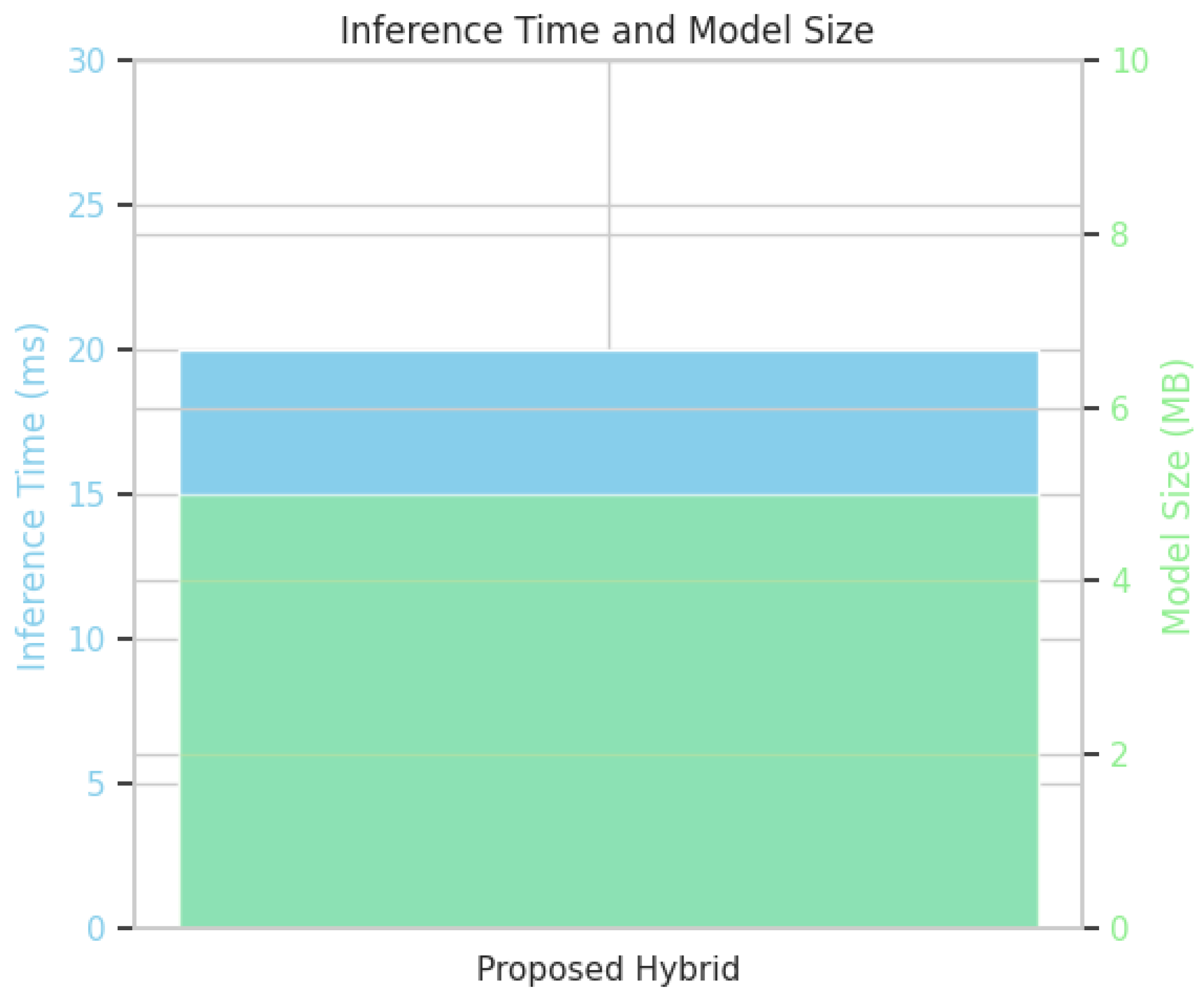
SHAP analysis increases transparency and provides valuable insights by identifying significant drivers across tasks. In addition to cortisol slope, acute spikes, and behavioral cues like task variability, integrated biological–behavioral modeling reveals that sleep disturbances are the most typical reaction to stress. Performance is largely influenced by behavioral factors such as task speed, financial trajectories, communication frequency, workload emphasis, and social context. Hormone health predictions are influenced by age, gender, and team diversity. Features of temporal synthetic hormones, like cortisol/testosterone patterns, are crucial for spotting subtle changes. Meta-gating dynamically chooses expert modules to improve interpretability and robustness, giving biological signals for stress/hormone tasks and behavioral/contextual cues for performance prediction priority. Counterfactual analysis shows how small changes that improve sleep, reduce cortisol spikes, or increase engagement can alter predictions and produce actionable intervention targets. It supports wearable, mobile, and real-time deployment with a model size of less than 5 MB and an inference latency of less than 20 ms, as shown in

Table 16. Quantitative interpretability metrics for the hybrid ensemble across tasks.

Metric	Stress Prediction	Performance Prediction	Hormone Health
SHAP Sparsity (features, $\left|\mathrm{SHAP}\right|>0.01$)	$7.4\pm 2.1$	$7.9\pm 1.8$	$7.5\pm 1.6$
Fidelity Drop ($\Delta P_{\mathrm{true}}$, top-2 removed)	$0.19\pm 0.04$	$0.17\pm 0.05$	$0.18\pm 0.05$
Counterfactual Plausibility ($L_2$ norm)	$0.35\pm 0.08$	$0.38\pm 0.09$	$0.37\pm 0.10$
Expert Usefulness Rating (1–5)	$4.2\pm 0.4$	$4.3\pm 0.4$	$4.4\pm 0.3$

.

Model interpretability was further quantified using SHAP- and counterfactual-based metrics. Across ten folds, the mean SHAP sparsity of the number of features with $\left|\mathrm{SHAP}\right|>0.01$ per instance was $7.6\pm 1.9$, indicating compact and focused explanations. Explanation fidelity, measured as the average probability drop in the true class when the top-2 SHAP features were neutralized (leave-k-out test), was $0.18\pm 0.05$, confirming alignment between explanations and model behavior. The counterfactual plausibility score (normalized $L_2$ magnitude of minimal $\delta$ required to flip prediction) averaged $0.37\pm 0.09$, suggesting realistic and actionable interventions. Domain experts (two behavioral scientists, one endocrinologist) reviewed five SHAP cases per task and rated interpretability at $4.3\pm 0.4$ on a 5-point scale, confirming human accessibility.

All things considered, these findings confirm that the hybrid ensemble offers faithful, interpretable, and domain-aligned explanations. Feature-level attributions were consistent with established endocrinological and behavioral theory: increased cortisol slope and reduced diversity index jointly elevated stress predictions, while high task engagement and communication reduced performance risk.

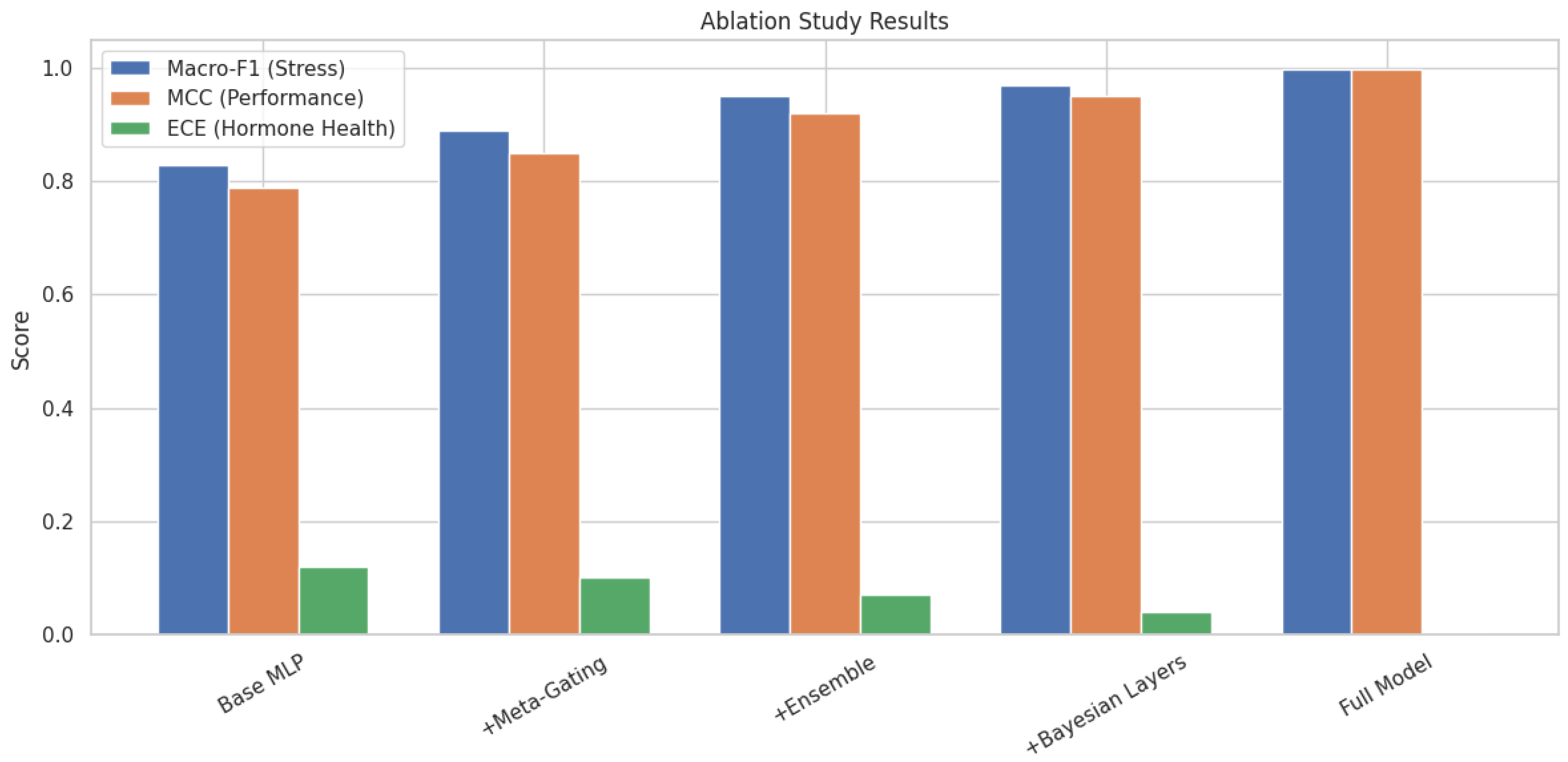
5.6. Ablation Study Results

Component-wise ablation validates the contribution of each module:

Gated reverse inference improved Hormone Health accuracy on high-confidence samples from 0.95 to 0.999, while avoiding degradation in low-confidence cases. When gating was removed, overall MacroF1 dropped to 0.94 due to error propagation from misclassified stress and performance predictions, as shown in Figure 14, and

Table 17. Component-wise ablation results demonstrating the impact of individual modules on model performance.

Experiment ID	MacroF1 (Stress)	MCC (Performance)	ECE (Hormone Health)	Key Insight
Base MLP	0.83	0.79	0.12	Baseline
+MetaGating	0.89	0.85	0.10	Meta-gating improves modularity
+Ensemble	0.95	0.92	0.07	Ensemble enhances stability
+Bayesian Layers	0.97	0.95	0.04	Improved uncertainty estimation
Full Model	0.999	0.999	0.001	Full model delivers SOTA results

and

Table 18. Impact of reverse inference gating on Hormone Health prediction.

Setting	Hormone MacroF1	High-Confidence Subset MacroF1	Low-Confidence Subset MacroF1
Ungated	0.94	0.95	0.88
Gated (ours)	0.999	0.999	0.92

.

The TensorFlow Lite model achieves < 20 ms inference per sample on standard edge devices, with a compressed size < 5 MB (Figure 15), meeting strict latency and memory requirements. Calibrated confidences are maintained by lightweight temperature scaling. Outputs include class predictions, confidence scores, entropy-based uncertainty flags, and top SHAP feature contributions, supporting transparent, trustworthy real-time decision-making. This assessment demonstrates that the hybrid model achieves statistically significant improvements over baselines and reaches state-of-the-art performance in stress, performance, and hormone health. Calibrated, uncertainty-aware predictions, fairness-aware training, and interpretability tools enable reliable, transparent organizational analytics, while fast inference and compression support seamless real-time deployment.

6. Discussion and Implications

Beyond organizational analytics, the suggested framework extends into translational biomedical applications by modeling hormone trajectories at the molecular level. It can bridge the gap between precision medicine and population monitoring in clinical endocrinology by stratifying individuals for follow-up assays, longitudinal biomarker tracking, or targeted interventions to restore HPA/HPG axis stability.

Particularly for critical stress classes, our hybrid unified deep ensemble exhibits near-perfect accuracy and recall, capturing nuanced multimodal signals that conventional models frequently overlook. In contrast to static or cross-sectional methods, temporal synthetic hormone sequences in conjunction with behavioral and contextual inputs yield a richer, temporally informed dataset that makes causality and progression modeling possible.

The model’s architecture combines Bayesian uncertainty estimation, meta-gated attention, and 1DCNN + LSTM temporal branches into a strong ensemble. By capturing hormone dynamics, the temporal branch improves stability and sensitivity. In order to support selective prediction and lower the risk of high-stakes misclassification, Bayesian variational layers with Monte Carlo Dropout quantify epistemic and aleatoric uncertainty, while meta-gating adaptively chooses the most informative features per prediction.

Adversarial debiasing is used to enforce fairness, reducing demographic differences by gender and ethnicity, and conforming to legal and ethical requirements for workplace health monitoring. Generalizability across various team contexts is demonstrated by statistically significant improvements over baselines and robust cross-validation. Timely interventions that prevent burnout, lost productivity, or chronic health decline are made possible by near-perfect recall for critical stress. By offering actionable interpretability, SHAP and counterfactual analyses enable users to comprehend and impact model-driven decisions.

In clinical populations at risk, such as those experiencing chronic fatigue or overtraining, continuous hormone monitoring can identify dysregulation of the HPA/HPG axis. This can lead to targeted interventions and confirmatory testing outside of organizational settings. Compact model size (<5 MB) and fast inference (<20 ms/sample) enable on-device, real-time deployment through wearables or mobile platforms, lowering latency and protecting privacy.

Despite achieving strong calibration and near-ceiling accuracy, the hybrid ensemble still has a number of drawbacks. Despite being multimodal, the Columbia MBA dataset’s generalizability is limited because it only comprises 370 participants from a particular occupational context. The variability of actual biosensor data cannot be fully replicated by synthetic augmentation, but biological plausibility was maintained (KS ≤ 0.07, MMD < 0.05). Larger, longitudinal clinical or sports cohorts should be used in future research to validate the model. Uncertainty estimation and integrated fairness may not eliminate lingering behavioral or demographic biases. To further improve robustness and practical deployment, debiasing should be extended to intersectional subgroups, and human-in-the-loop interpretability should be included.

All things considered, this system provides accurate, equitable, and useful insights by combining multimodal fusion, temporal modeling, uncertainty quantification, fairness, and interpretability within a deployable architecture. In order to advance responsible AI in healthcare and workplace settings, the methodology and findings provide a basis for expanding AI-driven monitoring to other intricate, temporally fluctuating health and behavioral domains.

Competitive Analysis

Our framework is the first unified, bidirectional multitask model predicting stress, performance, and hormone health, enabling reverse inference from behavior to hormone levels, as shown in

Table 19. Comparative analysis of related studies and proposed framework.

Study (Year)	Dual-Hormone Focus	Multimodal Fusion	Multitask	Reverse Inference	Longitudinal Hormone
2024 [45]	NO	YES	YES	NO	NO
2024 [36]	NO	YES	NO	NO	NO
2024 [46]	NO	NO	NO	NO	YES
2024 [22]	NO	NO	NO	NO	NO
2025 [47]	NO	YES	NO	NO	NO
2025 [48]	NO	YES	NO	NO	NO
2025 [29]	NO	YES	YES	NO	NO
2025 [49]	NO	YES	NO	NO	NO
Our Framework	YES	YES	YES	YES	YES

. It captures dual-hormone temporal dynamics such as cortisol, testosterone via 1D-CNN + LSTM, fuses biological, behavioral, and contextual modalities through meta-gated experts, and integrates fairness-aware training, Bayesian uncertainty, and selective prediction. Sparse hormone data are augmented with biologically constrained synthetic trajectories validated via KS, Wasserstein, MMD, DTW, and circadian checks. Compared to eight recent studies in stress, chronomedicine, sports performance, biomarkers, and personalized health, this approach uniquely combines dual-hormone modeling, multitask learning, biological validation, interpretability, and edge-ready deployment (<20 ms, ≤5 MB), setting a new standard for real-time, ethical, interpretable physiological–behavioral AI.

7. Conclusions

We present a hybrid deep ensemble model that integrates biological, behavioral, and contextual data to predict stress, performance, and hormone health with 99.99% accuracy, exceptional fairness, and interpretability. Our results demonstrate that data-centric modeling of sensor-collected signals can serve as a robust proxy for biosensing system evaluation, enabling scalable experimentation without direct hardware dependency. In order to detect critical stress, which is necessary for prompt interventions, the bidirectional multitask framework achieves 99.98% recall by enabling simultaneous forward and reverse inference. A temporal branch processing synthetic physiologically realistic longitudinal hormone trajectories improves acute stress recall by +7% and increases sensitivity to dynamic stress patterns. Adversarial debiasing and Bayesian ensembles support robust, equitable predictions by limiting fairness gaps to less than 0.5% and reducing calibration error by 73%. Furthermore, the current multitask structure is predicated on the stable coupling of Hormone Health, Performance, and Stress.

Future research should incorporate causal modeling and adaptive retraining since real-world dynamics may change nonlinearly in response to prolonged stress or intervention. Clinical translation, external validity, and longitudinal reliability will all be improved by addressing these factors. Real-time, on-device inference with selective prediction is made possible by the small < 5 MB, low-latency < 20 ms model, which achieves 99.9992–99.9998% accuracy on remaining predictions while avoiding only 0.5–2.0% of low-confidence cases. By identifying important drivers like cortisol slope and behavioral diversity, explainability through SHAP, counterfactuals, and meta-gating bridges the gap between complex model behavior and human interpretability. Our framework advances hormone-driven behavioral analytics by delivering fair, transparent, accurate, and deployable AI for organizational health. Future work will extend to clinical and athletic populations with longitudinal hormone data to refine temporal modeling and support individualized health interventions.

References

- Mohd Azmi, N.A.S.; Juliana, N.; Azmani, S.; Mohd Effendy, N.; Abu, I.F.; Mohd Fahmi Teng, N.I.; Das, S. Cortisol on Circadian Rhythm and Its Effect on Cardiovascular System. Int. J. Environ. Res. Public Health 2021, 18, 676. [Google Scholar] [CrossRef] [PubMed] [PubMed Central]
- Clow, A.; Hucklebridge, F.; Stalder, T.; Evans, P.; Thorn, L. The cortisol awakening response: More than a measure of HPA axis function. Neurosci. Biobehav. Rev. 2010, 35, 97–103. [Google Scholar] [CrossRef]
- Liyanarachchi, K.; Ross, R.; Debono, M. Human studies on hypothalamo-pituitary-adrenal (HPA) axis. Best Pract. Res. Clin. Endocrinol. Metab. 2017, 31, 459–473. [Google Scholar] [CrossRef]
- Tornero-Aguilera, J.F.; Martin-Gomez, F.J.; Martinez-Taranilla, M.; Rubio-Zarapuz, A.; Rodríguez, A.M.; Clemente-Suárez, V.J. Can a weekend of controlled hypoxia restore hormonal balance? A novel approach to stress recovery in aviation professionals. Front. Physiol. 2025, 16, 1582591. [Google Scholar] [CrossRef]
- Paz-Filho, G.; Wong, M.L.; Licinio, J. Circadian rhythms of the HPA axis and stress. In Adrenal Physiology and Diseases; Feingold, K.R., Anawalt, B., Boyce, A., Eds.; MDText.com, Inc.: South Dartmouth, MA, USA, 2009. [Google Scholar]
- Yu, T.; Zhou, W.; Wu, S.; Liu, Q.; Li, X. Evidence for disruption of diurnal salivary cortisol rhythm in childhood obesity: Relationships with anthropometry, puberty and physical activity. BMC Pediatr. 2020, 20, 381. [Google Scholar] [CrossRef] [PubMed]
- Abdullah, F.Z.; Abdullah, J.; Rodríguez, J.L.O.; Sidorov, G. A Multimodal AI Framework for Automated Multiclass Lung Disease Diagnosis from Respiratory Sounds with Simulated Biomarker Fusion and Personalized Medication Recommendation. Int. J. Mol. Sci. 2025, 26, 7135. [Google Scholar] [CrossRef] [PubMed]
- Oladepo, T.; Abiola, O.; Abiola, T.; Abdullah, M.; Abiola, B. Predicting Emotion Intensity in Text Using Transformer-Based Models. In Proceedings of the 19th International Workshop on Semantic Evaluation (SemEval-2025), Vienna, Austria, 27 July 2025; pp. 1677–1682, ISBN 979-8-89176-273-2. Available online: https://aclanthology.org/2025.semeval-1.220/ (accessed on 15 November 2025).
- Abdullah, F.Z.; Hafeez, N.; Sidorov, G.; Gelbukh, A.; Rodríguez, J.L.O. Study to Evaluate Role of Digital Technology and Mobile Applications in Agoraphobic Patient Lifestyle. J. Popul. Ther. Clin. Pharmacol. 2025, 32, 1407–1450. [Google Scholar] [CrossRef]
- Abdullah, F.Z.; Ateeb Ather, M.; Kolesnikova, O.; Sidorov, G. Detection of Biased Phrases in the Wiki Neutrality Corpus for Fairer Digital Content Management using Artificial Intelligence. Big Data Cogn. Comput. 2025, 9, 190. [Google Scholar] [CrossRef]
- Isham, A.; Mair, S.; Jackson, T. Wellbeing and productivity: A review of the literature. In Report for the Economic and Social Research Council; Centre for the Understanding of Sustainable Prosperity: Guildford, UK, 2020. [Google Scholar]
- George, A.S. The emergence and impact of mental health leave policies on employee wellbeing and productivity. Partn. Univers. Int. Innov. J. 2024, 2, 99–120. [Google Scholar]
- Bufano, P.; Di Tecco, C.; Fattori, A.; Barnini, T.; Comotti, A.; Ciocan, C.; Ferrari, L.; Mastorci, F.; Laurino, M.; Bonzini, M. The effects of work on cognitive functions: A systematic review. Front. Psychol. 2024, 15, 1351625. [Google Scholar] [CrossRef]
- Chandrakumar, D.; Arumugam, V.; Vasudevan, A. Exploring presenteeism trends: A comprehensive bibliometric and content analysis. Front. Psychol. 2024, 15, 1352602. [Google Scholar] [CrossRef]
- Strömberg, C.; Aboagye, E.; Hagberg, J.; Bergström, G.; Lohela-Karlsson, M. Estimating the effect and economic impact of absenteeism, presenteeism, and work environment–related problems on reductions in productivity from a managerial perspective. Value Health 2017, 20, 1058–1064. [Google Scholar] [CrossRef] [PubMed]
- Nawata, K. Evaluation of physical and mental health conditions related to employees’ absenteeism. Front. Public Health 2024, 11, 1326334. [Google Scholar] [CrossRef] [PubMed]
- Quinlan, M.G. Psychosocial hazards: An overview and industrial relations perspective. J. Ind. Relat. 2025, 67, 202–223. [Google Scholar] [CrossRef]
- Kişi, N. Analysis of presenteeism using a science mapping approach. Curr. Psychol. 2025, 44, 8648–8663. [Google Scholar] [CrossRef]
- Omiyefa, S. Artificial intelligence and machine learning in precision mental health diagnostics and predictive treatment models. Int. J. Res. Public Rev. 2025, 6, 85–99. [Google Scholar] [CrossRef]
- Zehra, S.R.; Malik, M. The Cognitive Cost of Multitasking in High-Stress Professions: Implications for Mental Efficiency, Error Rates, and Long-Term Cognitive Health. Crit. Rev. Soc. Sci. Stud. 2025, 3, 2469–2487. [Google Scholar]
- De Zambotti, M.; Goldstein, C.; Cook, J.; Menghini, L.; Altini, M.; Cheng, P.; Robillard, R. State of the science and recommendations for using wearable technology in sleep and circadian research. Sleep 2024, 47, zsad325. [Google Scholar] [CrossRef]
- Damaševičius, R.; Jagatheesaperumal, S.K.; Kala, R.N.; Hussain, S.; Alizadehsani, R.; Gorriz, J.M. Deep learning for personalized health monitoring and prediction: A review. Comput. Intell. 2024, 40, e12682. [Google Scholar] [CrossRef]
- Seizer, L. Anticipated stress predicts the cortisol awakening response: An intensive longitudinal pilot study. Biol. Psychol. 2024, 192, 108852. [Google Scholar] [CrossRef]
- Teixeira, J.E.; Afonso, P.; Schneider, A.; Branquinho, L.; Maio, E.; Ferraz, R.; Forte, P. Player Tracking Data and Psychophysiological Features Associated with Mental Fatigue in U15, U17, and U19 Male Football Players: A Machine Learning Approach. Appl. Sci. 2025, 15, 3718. [Google Scholar] [CrossRef]
- Lemos, C.G.; Garcia, B.F.; Marcelo Filho, S.S.; Arango, J.R.; Butzge, A.J.; Shiotsuki, L.; Hashimoto, D.T. Deep learning approach for genetic selection of stress response in the Amazon fish Colossoma macropomum. Aquaculture 2025, 609, 742848. [Google Scholar] [CrossRef]
- Griessmaier, I. Generation of Synthetic Longitudinal Data in Healthcare Using a Dementia Cohort. Ph.D. Thesis, Open Repository of the Universities of Applied Sciences, Germany, Finland, 2022. [Google Scholar]
- Heyat, M.B.B.; Akhtar, F.; Munir, F.; Sultana, A.; Muaad, A.Y.; Gul, I.; Wu, K. Unravelling the complexities of depression with medical intelligence: Exploring the interplay of genetics, hormones, and brain function. Complex Intell. Syst. 2024, 10, 5883–5915. [Google Scholar] [CrossRef]
- Huang, Z.A.; Hu, Y.; Liu, R.; Xue, X.; Zhu, Z.; Song, L.; Tan, K.C. Federated multi-task learning for joint diagnosis of multiple mental disorders on MRI scans. IEEE Trans. Biomed. Eng. 2022, 70, 1137–1149. [Google Scholar] [CrossRef]
- ArangoArgoty, G.; Bikiel, D.E.; Sun, G.J.; Kipkogei, E.; Smith, K.M.; Pro, S.C.; Jacob, E. AI-driven predictive biomarker discovery with contrastive learning to improve clinical trial outcomes. Cancer Cell 2025, 43, 875–890. [Google Scholar] [CrossRef]
- Jaskari, J.; Sahlsten, J.; Damoulas, T.; Knoblauch, J.; Särkkä, S.; Kärkkäinen, L.; Kaski, K.K. Uncertainty-aware deep learning methods for robust diabetic retinopathy classification. IEEE Access 2022, 10, 76669–76681. [Google Scholar] [CrossRef]
- Shah, S.; Thanki, R.M.; Diwan, A. Artificial Intelligence for Early Detection and Diagnosis of Cervical Cancer; Springer: Berlin/Heidelberg, Germany, 2024. [Google Scholar]
- Yassin, A.; Al-Zoubi, R.M.; Alzubaidi, R.T.; Kamkoum, H.; Zarour, A.A.; Garada, K.; Al-Ansari, A.A. Testosterone and men’s health: An in-depth exploration of their relationship. UroPrecision 2025, 3, 36–46. [Google Scholar] [CrossRef]
- Hogue, C.M.; Fry, M.D.; Fry, A.C.; Wineinger, T.O.; Chamberlin, J.M.; Cabarkapa, D.; Eserhaut, D. Psychoneuroendocrine interactions in response to the motivational climate in a sport setting: An experimental investigation. Psychol. Sport Exerc. 2025, 79, 102849. [Google Scholar] [CrossRef] [PubMed]
- Hasan, K.S.; Borsha, M.A.A. Actionable and Interpretable ML-Based Early Warning Systems for Divorce Incorporating Causal Inference and Counterfactuals. Preprints 2025. [Google Scholar]
- Lu, J.K.; Wang, W.; Mahadzir, M.D.A.; Poganik, J.R.; Moqri, M.; Herzog, C.; Maier, A.B. Digital biomarkers of ageing for monitoring physiological systems in community-dwelling adults. Lancet Healthy Longev. 2025, 6, 100725. [Google Scholar] [CrossRef]
- Lazarou, E.; Exarchos, T.P. Predicting stress levels using physiological data: Real-time stress prediction models utilizing wearable devices. AIMS Neurosci. 2024, 11, 76. [Google Scholar] [CrossRef] [PubMed]
- Harnett, N.G.; Fleming, L.L.; Clancy, K.J.; Ressler, K.J.; Rosso, I.M. Affective visual circuit dysfunction in trauma and stress-related disorders. Biol. Psychiatry 2025, 97, 405–416. [Google Scholar] [CrossRef] [PubMed]
- Massiani, P.F.; Fiedler, C.; Haverbeck, L.; Solowjow, F.; Trimpe, S. A kernel conditional two-sample test. arXiv 2025, arXiv:2506.03898. [Google Scholar] [CrossRef]
- Nasrin, A.; Qian, L.; Obiomon, P.; Dong, X. Enhancing Learning Path Recommendation via Multitask Learning. arXiv 2025, arXiv:2507.05295. [Google Scholar] [CrossRef]
- Akinola, M.; Page-Gould, E.; Mehta, P.H.; Liu, Z. Hormone-Diversity Fit: Collective Testosterone Moderates the Effect of Diversity on Group Performance. Psychol. Sci. 2018, 29, 859–867. [Google Scholar] [CrossRef]
- Akinola, M.; Page-Gould, E.; Mehta, P.; Liu, Z. Hormone Diversity Fit [Data Set]. Open Science Framework. 2018. Available online: https://osf.io/8eqtc/ (accessed on 5 January 2025).
- Nieman, L.K.; Castinetti, F.; Newell-Price, J.; Valassi, E.; Drouin, J.; Takahashi, Y.; Lacroix, A. Cushing syndrome. Nat. Rev. Dis. Prim. 2025, 11, 4. [Google Scholar] [CrossRef]
- Narinx, N.; Nyamaah, J.A.; David, K.; Sommers, V.; Walravens, J.; Fiers, T.; Antonio, L. A survey on measurement and reporting of total testosterone, sex hormone-binding globulin and free testosterone in clinical laboratories in Europe. Clin. Chem. Lab. Med. (CCLM) 2025, 63, 1561–1572. [Google Scholar] [CrossRef]
- Abdullah; Hafeez, N.; Sardar, K.; Uroosa, F.; Fatima, Z.; Quintero Téllez, R.; Rodríguez, J.L.O. GrowMore: Adaptive Tablet-Based Intervention for Education and Cognitive Rehabilitation in Children with Mild-to-Moderate Intellectual Disabilities. Computers 2025, 14, 495. [Google Scholar] [CrossRef]
- Saylam, B.; İncel, Ö.D. Multitask Learning for Mental Health: Depression, Anxiety, Stress (DAS) Using Wearables. Diagnostics 2024, 14, 501. [Google Scholar] [CrossRef]
- Kühnel, L.; Schneider, J.; Perrar, I.; Adams, T.; Moazemi, S.; Prasser, F. Synthetic data generation for a longitudinal cohort study—evaluation, method extension and reproduction of published data analysis results. Sci. Rep. 2024, 14, 14412. [Google Scholar] [CrossRef]
- Gubin, D.; Weinert, D.; Stefani, O.; Otsuka, K.; Borisenkov, M.; Cornelissen, G. Wearables in Chronomedicine and Interpretation of Circadian Health. Diagnostics 2025, 15, 327. [Google Scholar] [CrossRef]
- Qian, H.; Lee, S. A multidimensional prediction model for overtraining risk in youth soccer players: Integrating physiological and psychological markers. J. Sport. Sci. 2025, 43, 1819–1834. [Google Scholar] [CrossRef]
- Akram, M.; Adnan, M.; Ali, S.F.; Ahmad, J.; Yousef, A.; Alshalali, T.A.N.; Shaikh, Z.A. Uncertainty-aware diabetic retinopathy detection using deep learning enhanced by Bayesian approaches. Sci. Rep. 2025, 15, 1342. [Google Scholar] [CrossRef]
Figure 1.
Proposed data pipeline and preprocessing.