Abstract
Social media has become an almost unlimited resource for studying social processes. Seasonality is a phenomenon that significantly affects many physical and mental states. Modeling collective emotional seasonal changes is a challenging task for the technical, social, and humanities sciences. This is due to the laboriousness and complexity of obtaining a sufficient amount of data, processing and evaluating them, and presenting the results. At the same time, understanding the annual dynamics of collective sentiment provides us with important insights into collective behavior, especially in various crises or disasters. In our study, we propose a scheme for identifying and evaluating signs of the seasonal rise and fall of emotional tension based on social media texts. The analysis is based on Russian-language comments in VKontakte social network communities devoted to city news and the events of a small town in the Nizhny Novgorod region, Russia. Workflow steps include a statistical method for categorizing data, exploratory analysis to identify common patterns, data aggregation for modeling seasonal changes, the identification of typical data properties through clustering, and the formulation and validation of seasonality criteria. As a result of seasonality modeling, it is shown that the calendar seasonal model corresponds to the data, and the dynamics of emotional tension correlate with the seasons. The proposed methodology is useful for a wide range of social practice issues, such as monitoring public opinion or assessing irregular shifts in mass emotions.
1. Introduction
Emotions attract close attention because they make a decisive contribution to attitudes toward events, objects, and people. Motivation and behavior are largely determined emotionally at both the individual and collective levels, so understanding emotional phenomena provides a more complete picture of social processes and mass actions. Tracking the changes in collective emotions allows us to predict people’s reactions to events [1] and prevent negative scenarios [2]. Monitoring based on data from social networks favorably differs from classical sociological and statistical methods in its unobtrusiveness and minimal time lag between an emotional shift and its identification. This expands the possibilities of a prompt response to the growth of negative moods in society [3]. In addition, several areas of public interest, including health, finance, entertainment, advertising, and culture, could potentially benefit from measuring human emotions on social media [4]. The importance of understanding collective sentiment increases dramatically in a crisis situation, as shown by natural and man-made disasters, as well as the COVID-19 pandemic [5,6].
In our work, mood is considered as a complex long-lived emotional phenomenon, the main component of which is emotional tension. Due to its duration, unlike the emotion itself, mood has long-term dynamics. There is some evidence that collective sentiment is subject to seasonal fluctuations, with fluctuations occurring from year to year. If this is true, then the seasonality of public sentiment should be taken into account in socio-political practice.
The focus of the study is on emotional tension as the simplest component of collective mood, and we do not consider emotional investment in mood in this paper. The purpose of our study is to answer the following questions:
- What methods are applicable to detect patterns of variation in multiple assessments of a population’s psychological states when observed over time?
- Do collective emotional tensions in reality have seasonal variations that can be tracked through social media content analysis?
To study the seasonality of emotional tension, we used text comments from users of the social network VKontakte. In particular, we collected data from the largest communities dedicated to local news and events in a small town in the Nizhny Novgorod region of Russia.
Modern monitoring tools allow for the collection and storage of data in the form of time series. Time series contain the necessary information about the dynamics of the processes generating them. General methods of time series analysis, as a rule, make it possible to answer many of the questions related to the nature of the occurrence and seasonality of the processes being studied.
The distinctive features of the time series obtained as a result of monitoring social networks are discreteness, non-stationarity, and high sensitivity to data changes, which complicates their modeling and the use of traditional methods of analysis [7,8,9,10,11].
We used a combined approach, which is more typical of data science. We combined different data analysis techniques into a single workflow. In this approach, we do not model the time series but take its values as the domain to define the functions that are used for analysis, thus eliminating the problem of data sensitivity.
The workflow includes steps such as a statistical method for categorizing data, exploratory data analysis (EDA), feature selection and identification of common patterns according to a new target variable, aggregation of data to model seasonal changes, identification of typical data properties through clustering, analysis of cluster properties, formulation, and the validation of seasonality criteria. As part of the workflow, an approach to modeling seasonality in a class of time-aggregated models is proposed, and the conditions for their compliance with the data and the criterion of seasonality on a specific dataset are formulated.
2. Related Works
Certain researchers have noted that conceptual inconsistencies have hampered progress in the field of mood research. Some streamlining of terminology and differentiation of emotional phenomena—which, in many NLP studies, are arbitrarily referred to as intentions, beliefs, feelings, emotions, mood, and sentiment—could play a significant role in improving the efficiency of analysis [12]. In particular, ref. [13] emphasized the difference between background sentiment (or mood) and rapid shifts in sentiment (or emotion), as well as the impossibility of accurately identifying sentiment shifts because the patterns of background sentiment evolution are largely ignored by existing methods.
The following is a summary of three issues related to mood research: the characteristics and structure of mood; the mood markers used in NLP; and mood duration and dynamics (including methods for recording mood swings).
Currently, the emotionality of online content is mainly studied in the form of transient emotions, while the background mood remains out of sight. Mood and emotion differ in many dimensions such as clarity, duration, intensity, stability, causality, and control [14]. For example, emotion is more intense, but mood is longer in time; emotion is triggered by a specific event or incident, but mood does not necessarily need a contextual stimulus; and mood is strongly influenced by several factors, such as environment, physiology, or mental state [12]. In addition, emotion is primarily associated with positive valence, while mood is primarily associated with negative valence [14].
Under the names of popular forms of sentiment [15], aggregate mood [16], collective mood [17], collective sentiment [18], background sentiment [13], etc., two types of mass mood studies can be distinguished: (1) where mood is analyzed in terms of positive and negative polarity, and the mood dynamics are related to the movement between the poles [18,19,20,21]; (2) where mood is studied as a set of feelings involving more than one emotion [22], and the mood dynamics are seen as changes in the corresponding emotions [23]. In such approaches, mood does not differ from emotion in duration and is labeled as a rapidly changing attribute [16] with a minute [24], hourly [25], daily, or—at best—weekly cycle of change [26,27,28]. But, psychologically, it is more correct to say that mood is stable for several weeks, which provides a basis for calling it a “chronic” emotional state [29].
In terms of duration, mood can be recognized as a psychological phenomenon with an annual cycle of change. Indeed, it is believed that mood and related behavior are strongly dependent on the time of year [30]. A strong argument for the seasonality of emotional fluctuations is Seasonal Affective Disorder (SAD)—a recurrent type of major depression. Typically, SAD begins in the fall and continues through the winter months. Less commonly, SAD causes depression in spring or early summer. Symptoms consist of a sad mood and low energy [31].
In 2012, the prevalence of diagnosed SAD ranged from 1% to 10% of the global population, and, in temperate zones, from 3% to 10%. Subsyndromal SAD with blurred symptoms was found in 6% to 20% of the temperate population [32]. The minimum percentage of people with syndromic and sub-syndromic forms of SAD in Russia as a whole was at least 9%. We do not know how this ratio has changed over the past decade, but it is unlikely that its decrease, if any, has been significant. In addition, in the fall and spring periods, exacerbations of other mental illnesses occur, which gives an additional surge of depressive, asthenic, neurotic, and hypochondriacal symptomatology in the patient population [30,33]. Thus, it is difficult to accurately estimate how many social media users suffer from various endogenous seasonal mood swings and how much they contribute to the total amount of content generated.
Many of the studies reviewed in [34] empirically proved that seasonal mood swings are common in the general population as well. For example, nearly 50% of non-depressed people reported experiencing some depressive symptoms in winter, and it seemed that almost everyone had the most happiness in spring; however, it was also found that worthlessness, suicidality, and aggression have a significant connection with the seasons [34,35,36,37].
In terms of user-generated content, an analysis of 509 million tweets written by 2.4 million people in 84 countries showed that a shorter day length is associated with less positive sentiment in tweets [38], and another analysis of 800 million tweets in the UK revealed peak sadness in winter [39]. A study of Russian users’ search queries, using the Google Trends application, for “depression”, “anxiety”, “panic attack”, etc., showed that seasonal variations in web searches repeat the spring–autumn peaks and summer–winter valleys of depressive disorders and anxiety–depressive disorders [40]. In contrast, the study of [18] did not statistically support seasonal sentiment changes in structurally stable Twitter communities. The authors suggested that, when sentiment in a community temporarily deviates strongly from its normal level, it can usually be associated with a significant identifiable event that has affected the community, sometimes an external news event—in other words, the detected spikes are emotion-dependent rather than mood-dependent. Thus, it is still unclear whether seasonality is more or less intrinsic to the general population, as some researchers claim, or whether it can only be detected in fairly specific groups, as others believe.
For NLP, sentiment remains a very noisy signal due to the subtlety of human language [18]. Indeed, many effective tools have been proposed to analyze sentiment in social media based on machine learning or lexicon [41]. However, although mood word lists, idioms, emoticons, negation words, linguistic rules, and mood polarity classification algorithms [23] have been used to extract emotions from user content, negation, irony, metaphorical, and contextual ways of expressing attitudes interfere with the analysis results.
In addition, the textual expression of mood is colored by a person’s peculiar vocabulary and style, as well as by the social context, including social norms, history, and common understanding [15]. As for machine learning, recently, there have been doubts about its direct suitability for solving many of the problems of the socio-humanities in general and text analysis in particular [42,43].
In contrast to approaches to mood as a generalized bipolar emotion or as a combination of emotions, our study treats mood structurally, as a variable complex of emotions and emotional tension [44]. Emotional tension is a less significant and well-defined component of mood than emotion, and it is experienced as a state ranging from apathy to agitation [45]. In a social context, increases in public emotional tension in the form of mass forms of hostility, social anxiety, panic, hysteria, and aggression are associated with irrational collective behavior, such as social protest [46]. For our purposes, we rely on the tradition of assessing emotional tension as a component of mood, and this is embedded in the widely used Profile of Mood States (POMS) questionnaire [47]. Studies using the POMS questionnaire have shown that emotional tension is an attribute of both individual and group mood [48,49,50].
The advantage of assessing emotional tension, rather than mood per se, is that it can be extracted by simpler and more reliable means than tone dictionaries and other lexical tools. Namely, a tense emotional state is revealed by the correlation of parts of speech—verbs, nouns, adjectives—and their forms in user-generated content [51]. Such markers are less dependent on the topic and form of communication and are much less consciously controlled, which increases the reliability of the results. We investigated emotional tensions in social media using the Trager coefficient, or the ratio of verbs to adjectives in text.
The Trager coefficient was proposed to measure the level of a person’s emotional stability [52]. Its norm is close to 1 (more precisely, 1.34 ± 0.05), and values above the norm indicate emotional arousal and other sthenic states. Low values indicate insecurity, dependence, and anxiety [53]. Trager’s coefficient correlates with mental stress [54], suicidality [55], schizophrenia and clinical depression [56,57], expressed civil identity [58], insincerity in communication [59], etc., and it can also be used directly to assess emotional tension [52]. We believe that the fluctuations in the Trager coefficient in user-generated content reflect the dynamics of emotional tension in a user’s mood structure.
The study of mood as a long-lasting emotional state requires special methods that allow for capturing and reflecting on the temporal patterns of ongoing processes. A useful tool for this purpose can be variation, the significance of which is now well known from the classical works of W. Shewhart, which laid the foundation for the widespread use of the statistical method for the continuous monitoring and diagnosis of ongoing processes [60,61] and statistical process control (SPC) [62]. It is the variation in the Trager coefficient described above and mentioned in [52] that is an indicator of the emotional state, so the use of Shewhart control charts are appropriate in this case.
Through using control charts based on variation values, one can divide the entire observation period into days differing in emotional intensity, and one can then attempt to identify seasonal patterns by examining the resulting categorical time series. This partition plays a key role in our scheme for seasonality searching since, after transforming the data into a categorical series, we can obtain a randomized sequence with more stable patterns than in the original data. The transition to a categorical time series makes it possible to confidently use both well-known methods for working with such objects, such as statistical methods [63,64,65] and newly developed ones. A general theory of such series is currently being actively developed [66,67]; researchers propose various practical techniques depending on the software used [68], some of which may be suitable for finding seasonality.
Different types of aggregation are often used to detect seasonality, i.e., by calendar period or by selected observations, within a sliding window [69]. In the second case, the choice of periods is associated with an integer optimization problem (a review of methods for solving such problems is given in [70]).
Seasonality modeling in the absence of comparative time series models is possible using clustering. Practical methods of clustering, in particular clustering based on model fitting, are given in [69] and are more fully presented in [70].
In our study, within the framework of the workflow, we identified the main problems that arise when determining the presence of seasonal changes in collective emotional tension. Using the example of a specific dataset, we present a possible way of solving them in this particular case. Moreover, because of the key transition to a categorical time series, it is possible to apply the abovementioned methods that are aimed at solving similar problems in the general case. Thus, we have answered the first question posed in this study.
3. Materials and Methods
3.1. Data and Text Processing
Data for the study were collected from the 5 largest and most active communities of the VKontakte social network, which are dedicated to local city news and events in a town with a population of less than 100 thousand in the Nizhny Novgorod region of Russia. The number of subscribers in these social media communities varies from 12 to 43 thousand.
The data were collected using the official API of VKontakte. All posts and comments from 21 December 2019 to 5 March 2023 were downloaded. We did not download information about specific users’ data. Only the message type (comment or post), message text, and date were retained. A total of 83,125 posts and 662,881 comments were collected. In the VKontakte social network, posts are messages written by community administrators—in our case, they are mostly news related to local events. Comments, on the other hand, are messages from the subscribers of these communities who comment on the posts. Only comments were considered for further analysis as they contain the text of users, while posts are published on behalf of the community.
During the data cleaning process, we removed all comments that did not contain letters of the Russian alphabet, removed all characters that were not letters of the Russian alphabet or punctuation marks, and removed outliers that exceeded the 99th percentile for the number of characters and the number of sentences. The parameters of the collected data after cleaning are presented in Table 1.

Table 1.
Parameters of the collected data.
In the next step, each comment was analyzed using TITANIS [71], which computes multi-level linguistic markers of texts. Those text markers that required a morphological annotation of words were based on the results of a MyStem [72] analysis. The Trager coefficient was calculated by dividing the number of verbs by the number of adjectives in each comment. These values were averaged for each day, thus forming the final dataset on which further experiments were performed. The dataset with the average Trager coefficient by date is available in [73].
3.2. Dataset Specification: Main Properties and Features
Let us consider the main characteristics of the data and their properties, and let us also use exploratory analysis to identify existing patterns in the data and attributes that may indicate the presence of seasonality.
3.2.1. Descriptive Statistics of the Dataset
The dataset comprises daily calculations of the Trager coefficient values recorded from 21 December 2019 to 5 March 2023. We have 1171 observations, arranged by time. The descriptive statistics show the proximity of the dataset to a normal distribution (see Table 2).
Table 2.
Descriptive statistics of the dataset.
Descriptive statistics provide a more detailed understanding of the characteristics of the data under study.
3.2.2. Main Properties
Figure 1 shows the fit of the dataset to a normal distribution.
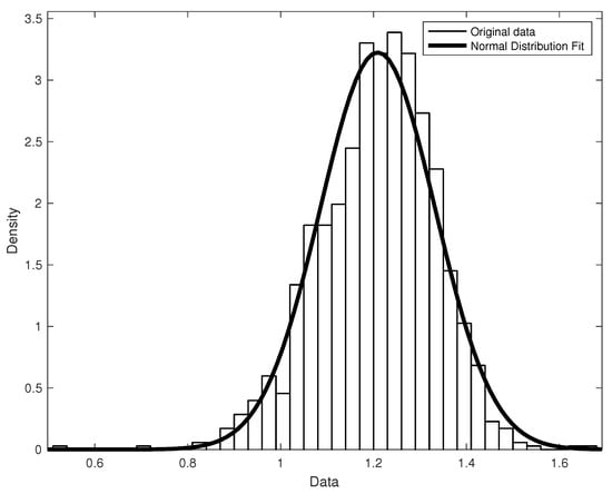
Figure 1.
This histogram visualizes the proximity of the dataset to a normal distribution. The MATLAB Distribution Fitter was used to fit the normal distributions to the data with Parameter Estimate: mu = 1.20889 (Std. Err. 0.00361506) and sigma = 0.123707 (Std. Err. 0.00255787).
By direct calculation, we verified that 68.66% of the data fit within one standard deviation of the mean, 95.64% were within two standard deviations of the mean, and 99.57% were within three standard deviations of the mean, which agrees quite well with the three-sigma rule (68–95–99.7). Table 3 shows the distribution of data by the area delineated by standard deviations: the number of records with values below one std (1 Std), one to two std (2 Std), two to three std (3 Std), and more than three std (out of 3 Std); the percentage of records by area; and the cumulative percentage by the areas of the data that fall within the intervals of up to one std, up to two std, and up to three std.
Table 3.
Data distribution through the standard deviation areas.
According to the three-sigma rule, the five values in the last row of Table 2 in the area “Out of 3 Std dev” are potential outliers or anomalies. These values do not affect the overall statistical properties, which are determined by more than 99% of the data. Here, we consider them to be simply values outside the standard deviation of the mean.
The properties of the studied dataset, recorded in Table 3, satisfy the basic control chart [74] and allow us to use the ideas of statistical method [61] for its dichotomy into categories. The simplest SPC method is a control chart, which presents the values grouped around a mean and the control limits. This is also known as the Shewhart [75] control chart. Using the control limits of the basic control chart, we transformed the data into a categorical time series, thereby assigning the category “white” to the values in the first area “1 Std dev” and the category “black” to the values in the remaining areas of Table 3.
Remark 1.
Note that through the key role of the dichotomy in the entire workflow, after transforming the data into a binary time series (categorical or, alternatively, a count series of zeros and ones), we obtain randomized sequences with more consistent patterns than those in the original data. Here, it is possible to use both purely statistical methods [63,64] and machine learning methods. Also, of undoubted interest, are the recent works by [68] on practical techniques with ordinal series and the works of [76,77] with count time series.
3.2.3. Dataset Features
Let us denote D as the time-ordered set of all records of the Trager coefficient values. Let us divide this set into two subsets: subset W (which contains records with values within one standard deviation of the mean) and . Now, we have set W with moderate variance and set B with high variance. Therefore, . According to Table 2, we see that, in set D, 68.66% of the elements are elements of set W and 31.34% of the elements are elements of set B. Therefore, we can determine the Base Level () of set D as 68.66% W (“Whites”) vs. 31.34% B (“Blacks”). For any subset of D similarly, we can determine the white level vs. black level () as a percentage of the number of elements for and ; thus, we can talk about the white-to-black ratio for . Now, we can compare the white-to-black ratios with the Base Level as for different samples.
Three-month cumulative samples for the entire observation period were considered according to seasonal, quarterly, and off-season samples: from February to April, from May to July, from August to October, and from November to January. Such samples reflected all the possible seasonal changes in the annual cycle.
The following charts show how the features of the D dataset manifested themselves in deviations in the white-to-black ratio from the Base Level for different calendar periods.
The diagram in Figure 2 is consistent with our idea of seasonal changes in emotional tension, i.e., that the persistence of emotional tension in winter and summer is statistically higher than in spring and fall. This suggests that the data properties may show signs of seasonality in the form of alternating dominant colors in a white-to-black ratio. If we take this as a sign of seasonality, then, in Figure 3, we can see signs of seasonality in the quarterly samples. Additionally, in Figure 4, we can see that the alternation in color dominance was already broken.
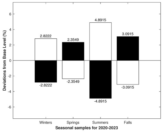
Figure 2.
The samples were based on records from 1 March 2020 to 28 February 2023. In the chart, the numbers at the ends of the bars indicate the deviation in the white-to-black ratios from the Base Level (). The seasonal samples from 2020 to 2023 show an alternation in white-to-black ratios, with black dominance in the spring and fall and white dominance in the winter and summer.
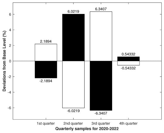
Figure 3.
The samples are based on records from 1 January 2020 to 31 December 2022. In the graph, the numbers at the ends of the bars indicate the deviation of the white-to-black ratios from the Base Level (). The quarterly samples from 2020 to 2022 show an alternation in white-to-black ratios, with black dominance in the second and fourth quarters and white dominance in the first and third quarters. From the first to the third quarter, the amplitude of deviations increases and falls sharply in the fourth quarter.
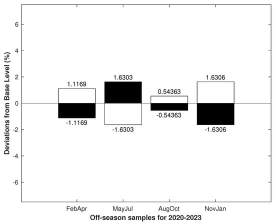
Figure 4.
The samples were based on records from 1 February 2020 to 31 January 2023. The numbers at the ends of the bars indicate the deviation in white-to-black ratios from the Base Level (). In the off-season samples, the alternation in the white-to-black ratio was broken. The predominance of white over black began in August and continued until January.
The presence of a characteristic in a cumulative sample does not mean that the seasonality property will be present in annual samples; meanwhile, the opposite is true, seasonality in the annual samples manifested itself in the aggregate ones, and the characteristic must be present in them. The disruption of the alternation in the off-season samples meant that these periods would not be considered further and that we can limit ourselves to annual seasonal and quarterly samples.
The following diagrams detail the distributions of subsets and for these calendar periods relative to the variable.
In Figure 5 and Figure 6, we see the manifestation of patterns in the alternation of changes in the white-to-black ratio over the selected periods. Such patterns can serve as signs of seasonality in the samples under consideration, but they do not provide an unambiguous answer about the nature of seasonality since they manifests themselves in both seasonal and quarterly intra-annual periods.
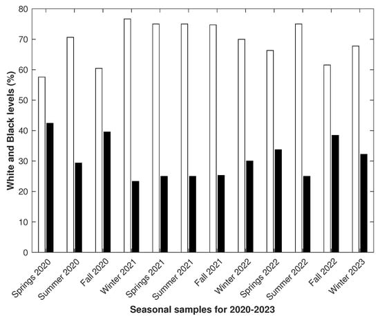
Figure 5.
The samples were based on records from 1 March 2020 to 28 February 2023. The seasonal alternation in white-to-black ratios () was typical from spring 2020 to spring 2021. The intervals from summer 2021 to autumn 2021 were approximately equal. Winter 2022 was an exception, after which the alternation was restored.
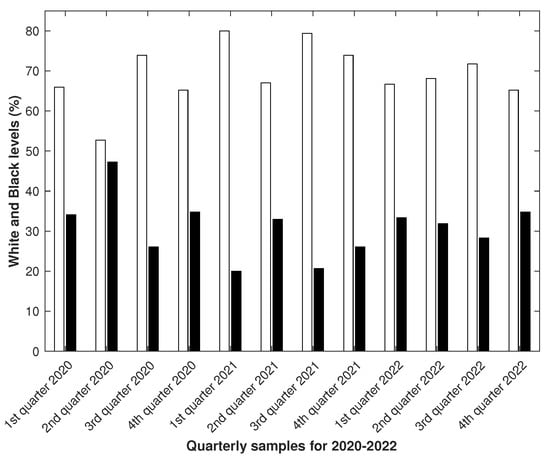
Figure 6.
The samples were based on records from 1 January 2020 to 31 December 2022. The quarterly alternation in white-to-black ratios () was typical from the first quarter of 2020 to the fourth quarter of 2021. The alternation sequence was broken from the fourth quarter of 2021 to the second quarter of 2022. The alternation was restored from the second quarter of 2022 to the fourth quarter of 2022, but with a noticeably smaller amplitude.
As a result of the primary analysis, patterns were identified in the data, thus indicating the presence of a certain common property (let us call it “seasonality”). This property of the data manifested itself in the form of alternating changes in white-to-black ratios in intra-year periods, both in the seasonal and quarterly samples, which did not allow them to be unambiguously localized in time and only on the basis of the considered statistical samples.
Features of the dataset allowed us to distinguish two types of patterns: one type based on calendar seasonal samples (Figure 5) and the other based on calendar quarterly samples (Figure 6).
Next, we modeled seasonality in the data, obtained a description of this property, and determined the criterion by which this property could be uniquely identified in the detected patterns. Let us check the feasibility of the criterion for each type of pattern, and, if the criterion satisfies any type, we will consider a seasonality model based on this type of pattern, check it for compliance with the data and for its adequacy in our understanding of seasonality.
3.3. Seasonality Modeling
Model Aggregated by Time-Duration
Recall that the dataset was divided into two subsets of white and black days (), and its Base Level () was 68.6593% white versus 31.3407% black, which is defined as
where , , and are the cardinalities of the sets W, B, and D, respectively.
The time-aggregated model (TAM) for dataset D is
where is the selected time intervals consisting of the number of full days, so the for each is an integer.
The number of elements in is represented by a pair of white and black days; therefore, for the cardinalities of the sets and for each , the white and black levels for were defined as a vector as follows:
where is a 2-vector composed of the cardinalities of the sets and , and the white and black level for TAM is
The condition for the model to match the data is
where is the Base Level of dataset D, and is the Euclidean norm of the vector.
3.4. Uniformly Aggregated TAMs
Let , , , , .
TAM, with the cardinalities of the sets for any , is uniformly aggregated if .
Statement 1.
Any uniformly aggregated TAM on some dataset D matches to the dataset.
Proof of Statement 1.
If , then
and so . □
Remark 2.
The time series is a trivial TAM case with .
Consider the subsets of the dataset D of 1170 days (for example, the records from 21 December 2019 to 4 March 2023, or the records from 22 December 2019 to 5 March 2023). For two subsets, the cardinality and their TAMs were as follows:
which corresponded with and .
Uniformly aggregated TAMs are useful for learning datasets because they can be extended to an arbitrary dataset. Let us designate the first model for the dataset with records from 21 December 2019 to 4 March 2023 as TAM1, and let us set the second model for the dataset with the records from 22 December 2019 to 5 March 2023 as TAM2. Let us see how these models behave across the entire dataset D.
3.5. Extension of Uniformly Aggregated TAMs on a Dataset
For dataset D with 1171 records from 21 December 2019 to 5 March 2023, we have , , , and . There are two ways to extend the uniformly aggregated TAM that is represented by (4) into the D dataset. We can interpret the TAM as a uniform k-lattice on top of the data with cells and add the missing data to the beginning or end of the lattice (by expanding cell or cell ), or by moving the lattice to the left or right and resizing the first and last cells.
3.5.1. Extending the Model by Adding Data
Uniformly aggregated TAM1 specifies the distribution of the white and black days in the form on a dataset of 1170 days. Consider the extended TAM1 with additional data on the right as follows:
Here, the r elements need to be added to the last cell , and, for the extended model, the new number of elements in will be , where x is a logical r-vector of 0 and 1, which indicates the presence of white and black elements in an additional interval of length r. The extended model does not have to fit the data exactly, but, for TAM, the error in condition (3) can be expressed in terms of the model parameters.
Now, we can express the Base Level of D for this decomposition as
and the white and black levels for extended TAM1 as
From (6) and (7), we can obtain
and, after bringing similar ones forward, we can find the error in matching the model to the data in the form
Similarly, for the extended TAM2 with additional data on the left, we can obtain
and we can find the error in matching the model to the data in the form
Substituting the parameter values , , and into Expressions (8) and (10), we obtain for the extended TAM1 (denote as ExTAM1) the error in matching the model to the data in (8), which is equal . For the extended TAM2 (denoted as ExTAM2), the error in matching the model to the data in (10) is equal . Thus, ExTAM1 fits the data on the set D slightly better than ExTAM2.
3.5.2. Expanding the Model by Shifting a Uniform Lattice on the Dataset
The principle of moving windows can be implemented in TAM by shifting a uniform lattice on the dataset. Let us consider a uniformly aggregated model with finite cells that are shifted by a distance l, where l is an integer of the form
This is similar to moving a conveyor belt, i.e., when a lattice is moved to the left by a distance l, the first cell goes beyond the boundary of the set D and its size decreases by l, but, at the same time, the last cell at the right end of the lattice increases by the same amount l.
For each l, we obtain a new distribution of white and black days across cells in the form on a dataset D; thus, we can express the BaseLevel of D for each decomposition as
and the white and black levels for (11) as
The condition for the model to match the data in (3) takes the form
and, after bringing similar ones forward, we can find an expression that connects the error in matching the model with the data with the model parameters as follows:
Remark 3.
Note that the shift method identifies models that better fit the data. For example, a model of type (11) with parameter values , , , and (denoted as ShTAM3) from the expression (12) has a model-to-data matching error of . A model of type (11) with parameter values , , , and (denoted as ShTAM10) from Expression (12) has a best model-to-data fitting error of ≈0.0002.
3.5.3. Evaluating and Comparing Models on the Real Dataset
Let us estimate the fitting errors of the seasonality models on the entire dataset D, which was described above. Let us consider models with parameter values , , and , as well as vary the parameter l from to 41 so that the minimum sizes of the end cells are not less than 50 (the starting point here corresponds to 90 days from the moment of the first record). The best-fitting models with matching errors of less than are presented in Table 4.
Table 4.
Ranking models according to the data fit.
Note the three isolated local minima with , , and , as well as a robust local minimum with .
Let denote the set consisting of the parameter values of the best-fitting models from Table 4. As such, .
Let be an output of the shift model (11) with parameters l and k, then , , where the for each i is defined in (2) for the corresponding model.
Let us form a cluster on the set of the best-fitting models using the idea of the centroid method. In the first iteration, we build a centroid
by averaging the white and black levels for all the models from set . The R-squared () and MAPE metrics were used to estimate the distance for each model from the set to the centroid.
After the first iteration, the models with parameter values () and () were excluded as the two worst on the -metric.
In the second iteration, two of the models with fit errors of and were added because their parameter values of and were inside the new cluster. Models with parameter values of (), (), (), and ( 0.9790) were then excluded based on the -metric being less than .
At the third iteration, a final cluster of thirteen models () was formed (Table 5) around a centroid whose matching error to the data was .
Table 5.
Comparison of models by their closeness to the centroid.
A visualization of the final centroid using a bar chart gives a characteristic visual picture of the dataset in Figure 7, which most closely matches the distribution of black and white days for the models in the cluster.
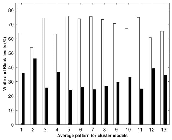
Figure 7.
The centroid was an array , the values of the components of which were determined by the formula (13) by averaging the white and black levels for all the models from the set with . Therefore, the axis shows the indices of the array elements, and the axis shows the values of the array elements. For each index , the value of the array element was a pair consisting of white and black values corresponding to this index.
3.5.4. Cluster Properties
The models united in a cluster have common properties. As an example, Figure 8 shows bar charts with a similar pattern for the two models from the cluster with parameters and , which were located at opposite ends of the cluster.
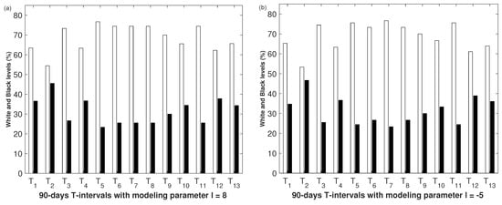
Figure 8.
Black and white ratios on the intervals. The axis shows the intervals corresponding to the model, and the axis shows the white and black levels for , which was determined by Formula (2). (a) Model with parameter value ; (b) model with parameter value .
Figure 7 and Figure 8 clearly show stable alternations in white-to-black ratios on the intervals – and –, which persist when the data distributions over the intervals change with the model. It was also clearly visible that the main differences in the ratio of white and black appeared at the intervals —, which is when small fluctuations were observed in the level of white and black leading to visual changes in this part of the picture. This was true for all models in the cluster.
Let us look, in detail, at the behavior of the cluster models in the range –. Figure 9 graphically shows fragments of the output values for all the thirteen cluster models, i.e., for all .
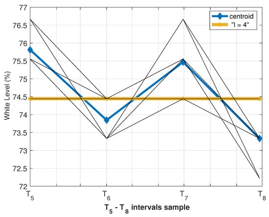
Figure 9.
Comparative behavior of the intervals from to . Values of the white levels in the output components in the points for all . Some of the lines overlapped each other, so there appeared to be fewer than thirteen lines.
Figure 9 highlights two “trends”—the blue line of the centroid, which determines the direction for most models, and the yellow line of the “boundary” model with parameter , for which all values were equal.
Let us denote this extreme value as and focus on an important property of the cluster, which we describe for white levels in the output as follows:
The conditions (14) indicated that the alternations in white-to-black ratios were not violated in the range of —.
Taking into account Equation (14), the alternation conditions on the entire dataset, i.e., in the range —, for the model with parameter l were written in the form
where denotes the integer part of the real number.
Let us formalize this result in the form of a criterion that allows us to unambiguously determine whether a given model of type (1) corresponds to the seasonality property of the data. As such, the following theorem is true.
Theorem 1 (Data seasonality compliance criteria).
Let us say that the time-aggregated model (1) with parameter and for all , corresponds to the data seasonality on dataset D. Then, if the white-to-black ratio in Equation (2) for T satisfy one of Conditions (17) or (18), we have
where and , and denotes the integer part of the real number.
Theorem 1 establishes the necessary conditions for the pattern to correspond to the data seasonality property.
4. Results
At the beginning of this paper, the objectives of our study were formulated to answer two questions:
- (1)
- What methods are applicable to detect patterns of variation in multiple assessments of a population’s psychological states when observed over time?
- (2)
- Do collective emotional tensions in reality have seasonal variations that can be tracked through social media content analysis?
To answer the first question, let us list the workflow steps used in this paper to identify the patterns of change in the psychological state of the population: statistical method and exploratory data analysis based on descriptive statistics; definition of new functions to identify patterns in the data; formulation of the modeling problem; data aggregation; use of the clustering method to identify typical properties of the data; formulation of the soft sign criterion of “seasonality” (based on the analysis of data typical properties); and the demonstration of the manifestation of “data-seasonality” in the calendar seasonal model.
The affirmative answer to the second question is based on the following results:
- As a result of the analysis of the statistical data, features of the data array were identified that make it possible to display mass emotional tension in the ratio of whites and blacks in selected calendar periods;
- The proposal of an approach to model seasonality in a class of time-aggregate models;
- Within the framework of the above proposed approach, it was shown that the data were characterized by the property of “data seasonality”, and the description of this property was obtained in the form of a stable pattern for all models from the found cluster;
- Based on the identified features of data seasonality, a criterion for matching this property for other time aggregated models was formulated.
In a direct test of the seasonality of the compliance criteria (Theorem 1), it was shown that the pattern on calendar seasonal samples (Figure 5) satisfies condition (17), while the seasonality data fit criterion was not met for the pattern on calendar quarterly samples (Figure 6).
The diagram in Figure 10 shows a calendar seasonal model pattern that extended to the entirety of dataset D, which corresponded with the data seasonality property (see Figure 7 for visual confirmation).
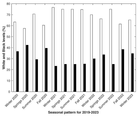
Figure 10.
Seasonal pattern according to the calendar seasonal model across the dataset based on records from 21 December 2019 to 5 March 2023.
This means that the calendar seasonal pattern was consistent with the data, and the alternating white-to-black ratios fit well with our understanding of how the overall dynamics of emotional tension correlate with the seasons.
5. Discussion
From a psychological point of view, two of the results were the most significant.
First, the obtained data confirmed the general seasonal dynamics of emotional tension to be traceable in the analysis of network communications. Indicators of emotional tension stability were statistically significantly higher in winter and summer than in spring and fall (see Figure 2 and Figure 10). We found that the indicator of collective emotional tension varied strongly from day to day more often in spring and fall than in winter and summer. The revealed dynamics corresponded well with the above-described trends of changes in emotional state, which were revealed in psychiatric and psychological practice or in the course of sociological surveys.
Second, we found the absence of spring and fall peaks in the dynamics of emotional tension in 2021. In contrast to 2020 and 2022 (where there were pronounced differences between the more stable winter and summer on the one hand, and the more volatile spring and fall on the other), the level of differences in emotion tension in 2021 remained relatively unchanged across all four seasons. The available data did not allow us to infer the nature of this equalization. The cause could be either constant fatigue and apathy or, conversely, constant excitement and overexcitement during the second year of the pandemic. Thus far, we can only point to an atypical pattern of seasonal dynamics of emotional tension in 2021 if we take the winter–spring and summer–fall differences as typical. Based on the idea of the endogenous nature of seasonal fluctuations of mood (and emotional tension as its component), we can assume that in the first year the dynamics are still intact, and in the third year it is somewhat restored.
A pandemic is a prolonged stressor that disrupts the normal life of the population and undoubtedly affects mass psychiatric conditions. At the outset of the pandemic, an excessive impact on mental functioning was identified and a further increase in psychopathologic symptoms was predicted [78]. However, defense mechanisms (such as threat underestimation [79] or humor [80]) kept psychological states inert for some time. A possible basis for the recovery of mass mental functions is adaptation to prolonged stressors [21]. Thus, the detected pattern of collective emotional tension can be explained as a result of the action of defense mechanisms in 2020, the disorder of adaptation of the population to a long-term stressor in 2021, and gradual adaptation to extreme conditions in 2022.
The presented scheme for determining seasonality may be of interest for various social practices. For example, by accumulating data on the severity of fluctuations in emotional tension in different regions, it will be possible to identify regions with an increased risk of chaotic mass behavior during periods of seasonal exacerbations. It is also useful to predict the possible deterioration of the collective emotional state in order to optimize the work of various social services that may face an increased flow of requests during unfavorable periods. It is possible to link the seasonality of emotional tension with the manifestation of mass somatic or mental disorders affecting the economic and social functioning of regions, etc.
Limitations and Future Work
This study raised many questions. We studied collective sentiment averaged over a large number of social media users. We do not know whether only users with pronounced emotional seasonal shifts affected the overall emotional tension in the network while others did not affect the tension at all, or whether all users contributed to some degree to the overall emotional tension online. To clarify this question, a special longitudinal study involving the identification of people with different emotional statuses is needed. For a meaningful characterization of “black days”, it is necessary to distinguish between days in which an instability of emotional tension is caused by a significant upward trend of the Trager coefficient (spikes of overexcitement) or a significant downward trend (spikes of apathy). Verification of the identified seasonal trends is possible both with the help of other methods for assessing emotional tension in online communication and by building up more texts for analysis. A promising direction for further research is to determine the emotional component of mood in addition to the assessment of emotional tension.
It should be noted that this study was conducted using data from one local social media community, which could potentially introduce bias. Thus, observations in other communities could show a different picture. In addition, this paper only considers the Trager coefficient to assess emotional tension, whereas our method could potentially be applied to other normally distributed psycholinguistic parameters. These limitations should be addressed in future work.
6. Conclusions
In this paper, we proposed a combined approach for detecting the seasonality of emotional tension in social media based on the statistical method for data categorization, exploratory data analysis to identify general patterns, modeling seasonality in the class of time-aggregated models (TAM), and identifying typical properties of TAM data using the clustering method. It was shown that the dynamics of emotional tension correlate with the seasons of the year. To the best of our knowledge, this is the first study to investigate the task of detecting seasonality in emotional tension using social media data. To assess emotional tension, we used the Trager coefficient, which has not previously been used in this task. We look forward to using the proposed method to account for the seasonality of emotional tension when analyzing relationships between non-seasonal shifts in emotional tension, specific events, and the content of social media texts.
Our results suggest that the emotional tension manifested in social media communication tends to fluctuate with the seasons, but strong and long-lasting stressors can distort seasonality. The proposed methodology for identifying, evaluating, and displaying the dynamics of emotional tension based on network communications demonstrates sensitivity to both stable annual fluctuations and the external influences that disrupt them. However, further development of the method will require more data, longer observation periods, and data from other social media communities.
Author Contributions
Conceptualization, Y.K. and I.S.; methodology, A.N. and Y.K.; software, M.S.; validation, A.N.; formal analysis, A.N.; investigation, A.N.; data curation, M.S.; writing—original draft preparation, A.N., Y.K. and M.S.; writing—review and editing, I.S. and O.G.; visualization, A.N.; supervision, I.S.; project administration, I.S. and O.G.; funding acquisition, O.G. All authors have read and agreed to the published version of the manuscript.
Funding
This work was supported by the Ministry of Science and Higher Education of the Russian Federation (project No. 075-15-2020-799).
Institutional Review Board Statement
Ethical approval is not required for this paper, as the data used in this paper were collected and processed in accordance with the Federal Law of the Russian Federation No. 149-FZ of 27 July 2006 “On Information, Information Technologies and Protection of Information”. The data presented in this study contain only numerical values and cannot be used to reveal any real identities.
Data Availability Statement
The data presented in this study are openly available in the Hugging Face repository at https://doi.org/10.57967/hf/1475 (Accessed on 21 December 2023).
Conflicts of Interest
The authors declare no conflicts of interest.
Abbreviations
The following abbreviations are used in this manuscript:
| EDA | Exploratory Data Analysis |
| NLP | Natural Language Processing |
| SPC | Statistical Process Control |
| TAM | Time-Aggregated Model |
| SAD | Seasonal Affective Disorder |
| API | Application Programming Interface |
| MAPE | Mean Absolute Percentage Error |
References
- Nguyen, L.T.; Wu, P.; Chan, W.; Peng, W.; Zhang, Y. Predicting Collective Sentiment Dynamics from Time-series Social Media. In Proceedings of the First International Workshop on Issues of Sentiment Discovery and Opinion Mining, Beijing, China, 12 August 2012; pp. 1–8. [Google Scholar] [CrossRef]
- Giachanou, A.; Mele, I.; Crestani, F. Explaining Sentiment Spikes in Twitter. In Proceedings of the 25th ACM International on Conference on Information and Knowledge Management, Indianapolis, IN, USA, 24–28 October 2016; pp. 2263–2268. [Google Scholar] [CrossRef]
- Grebenuyk, A.; Maksimova, A.; Lemer, L. Study of Social Tension Based on Electronic Social Networks Big Data. Digit. Sociol. 2021, 4, 4–12. (In Russian) [Google Scholar] [CrossRef]
- De Choudhury, M.; Counts, S. The Nature of Emotional Expression in Social Media: Measurement, Inference and Utility; Human Computer Interaction Consortium (HCIC): Minneapolis, MN, USA, 2012. [Google Scholar]
- Abdukhamidov, E.; Juraev, F.; Abuhamad, M.; El-Sappagh, S.; AbuHmed, T. Sentiment Analysis of Users’ Reactions on Social Media During the Pandemic. Electronics 2022, 11, 1648. [Google Scholar] [CrossRef]
- Abdul Mueez, A.; Mardiana, O.; Rosliza, A. Role of Social Media in Disaster Management. Int. J. Public Health Clin. Sci. 2019, 6, 77–99. [Google Scholar]
- Holt, C.C. Forecasting Seasonals and Trends by Exponentially Weighted Moving Averages. Int. J. Forecast. 2004, 20, 5–10. [Google Scholar] [CrossRef]
- Winters, P.R. Forecasting Sales by Exponentially Weighted Moving Averages. Manag. Sci. 1960, 6, 324–342. [Google Scholar] [CrossRef]
- Brockwell, P.; Davis, R. Introduction to Time Series and Forecasting; Springer: Cham, Switzerland, 2016; p. 425. [Google Scholar] [CrossRef]
- Hyndman, R.; Athanasopoulos, G. Forecasting: Principles and Practice, 3rd ed.; OTexts: Melbourne, Australia, 2021. [Google Scholar]
- United Nations Economic Commission for Europe. Practical Guide to Seasonal Adjustment with JDEMETRA+: From Source Series to User Communication; UNECE: Geneva, Switzerland, 2020; p. 95. [Google Scholar] [CrossRef]
- Ragheb, W. Affective Behavior Modeling on Social Networks. Ph.D. Thesis, Université Montpellier, Montpellier, France, 2020. [Google Scholar]
- Wang, Y.; Li, H.; Lin, C. Modeling Sentiment Evolution for Social Incidents. In Proceedings of the 28th ACM International Conference on Information and Knowledge Management, Beijing, China, 3–7 November 2019; pp. 2413–2416. [Google Scholar] [CrossRef]
- Beedie, C.; Terry, P.; Lane, A. Distinctions Between Emotion and Mood. Cogn. Emot. 2005, 19, 847–878. [Google Scholar] [CrossRef]
- Nguyen, T.; Phung, D.; Adams, B.; Venkatesh, S. Mood Sensing from Social Media Texts and its Applications. Knowl. Inf. Syst. 2014, 39, 667–702. [Google Scholar] [CrossRef]
- Mishne, G.; De Rijke, M. Capturing Global Mood Levels using Blog Posts. In Proceedings of the AAAI Spring Symposium: Computational Approaches to Analyzing Weblogs, Stanford, CA, USA, 27–29 March 2006; Volume 6, pp. 145–152. [Google Scholar]
- Greetham, D.V.; Sengupta, A.; Hurling, R.; Wilkinson, J. Interventions in Social Networks: Impact on Mood and Network Dynamics. Adv. Complex Syst. 2015, 18, 1550016. [Google Scholar] [CrossRef]
- Charlton, N.; Singleton, C.; Greetham, D.V. In the Mood: The Dynamics of Collective Sentiments on Twitter. R. Soc. Open Sci. 2016, 3, 160162. [Google Scholar] [CrossRef]
- He, Y.; Lin, C.; Gao, W.; Wong, K.F. Tracking Sentiment and Topic Dynamics from Social Media. In Proceedings of the International AAAI Conference on Web and Social Media, Dublin, Ireland, 4–7 June 2012; Volume 6, pp. 483–486. [Google Scholar] [CrossRef]
- Patel, K.; Hoeber, O.; Hamilton, H.J. Real-time Sentiment-based Anomaly Detection in Twitter Data Streams. In Proceedings of the Advances in Artificial Intelligence: 28th Canadian Conference on Artificial Intelligence, Canadian AI 2015, Halifax, NS, Canada, 2–5 June 2015; Proceedings 28. Springer: Cham, Switzerland, 2015; pp. 196–203. [Google Scholar] [CrossRef]
- Wang, H.; Sun, K.; Wang, Y. Exploring the Chinese Public’s Perception of Omicron Variants on Social Media: Lda-based Topic Modeling and Sentiment Analysis. Int. J. Environ. Res. Public Health 2022, 19, 8377. [Google Scholar] [CrossRef]
- Lane, A.M.; Terry, P.C. The Nature of Mood: Development of a Conceptual Model with a Focus on Depression. J. Appl. Sport Psychol. 2000, 12, 16–33. [Google Scholar] [CrossRef]
- Alam, F.; Celli, F.; Stepanov, E.; Ghosh, A.; Riccardi, G. The Social Mood of News: Self-reported Annotations to Design Automatic Mood Detection Systems. In Proceedings of the Workshop on Computational Modeling of People’s Opinions, Personality, and Emotions in Social Media (PEOPLES), Osaka, Japan, 12 December 2016; pp. 143–152. [Google Scholar]
- Jome Yazdian, P.; Moradi, H. User Mood Detection in a Social Network Messenger Based on Facial Cues. In Proceedings of the Ubiquitous Computing and Ambient Intelligence: 11th International Conference, UCAmI 2017, Philadelphia, PA, USA, 7–10 November 2017; Proceedings. Springer: Cham, Switzerland, 2017; pp. 778–788. [Google Scholar] [CrossRef]
- Meyer, J.D.; Murray, T.A.; Brower, C.S.; Cruz-Maldonado, G.A.; Perez, M.L.; Ellingson, L.D.; Wade, N.G. Magnitude, Timing and Duration of Mood State and Cognitive Effects of Acute Moderate Exercise in Major Depressive Disorder. Psychol. Sport Exerc. 2022, 61, 102172. [Google Scholar] [CrossRef]
- Balog, K.; Mishne, G.; De Rijke, M. Why Are They Excited? Identifying and Explaining Spikes in Blog Mood Levels. In Proceedings of the 11th Conference of the European Chapter of the Association for Computational Linguistics, Trento, Italy, 3–7 April 2006; pp. 207–210. [Google Scholar]
- Lee, J.A.; Efstratiou, C.; Bai, L. OSN Mood Tracking: Exploring the Use of Online Social Network Activity as an Indicator of Mood Changes. In Proceedings of the 2016 ACM International Joint Conference on Pervasive and Ubiquitous Computing: Adjunct, Heidelberg, Germany, 12–16 September 2016; pp. 1171–1179. [Google Scholar] [CrossRef]
- Smetanin, S.I. The Program for Public Mood Monitoring through Twitter Content in Russia. Proc. ISP RAS 2017, 29, 315–324. [Google Scholar] [CrossRef][Green Version]
- Maklakov, A. Obshchaya Psikhologiya [General Psychology]; Piter Publisher: Saint Petersburg, Russia, 2001. (In Russian) [Google Scholar]
- Winthorst, W.H.; Bos, E.H.; Roest, A.M.; de Jonge, P. Seasonality of Mood and Affect in a Large General Population Sample. PLoS ONE 2020, 15, e0239033. [Google Scholar] [CrossRef]
- Melrose, S. Seasonal Affective Disorder: An Overview of Assessment and Treatment Approaches. Depress. Res. Treat. 2015, 2015, 178564. [Google Scholar] [CrossRef]
- Khaustova, Y. Seasonal Affective Disorder: Diagnosis and Therapy. Int. Neurol. J. 2012, 48, 188–192. (In Russian) [Google Scholar]
- Buikov, V.; Kolmogorova, V.; Burtova, E. Preventivny’e Lechebny’e Mery’ v Osenne-vesennij Period u Obluchennogo Naseleniya na Yuzhnom Urale [Preventive Therapeutic Measures in the Autumn-spring Period in the Irradiated Population of the Southern Urals]. Human. Sport. Med. 2007, 74, 48–51. (In Russian) [Google Scholar]
- Hohm, I.; Wormley, A.S.; Schaller, M.; Varnum, M.E. Homo Temporus: Seasonal Cycles as a Fundamental Source of Variation in Human Psychology. Perspect. Psychol. Sci. 2023, 1–22. [Google Scholar] [CrossRef]
- Palmu, R.; Koskinen, S.; Partonen, T. Seasonal Changes in Mood and Behavior Contribute to Suicidality and Worthlessness in a Population-based Study. J. Psychiatr. Res. 2022, 150, 184–188. [Google Scholar] [CrossRef]
- Rozanov, V.; Grigoriev, P.; Sumarokov, Y.; Shelygin, K.; Karyakin, A.; Malyavskaya, S.; Sidorenkov, O. Analysis of Seasonal Variations of Suicides in the Archangelsk Region in Relation to Geoclimatic Factors. Suicidology 2019, 10, 82–91. (In Russian) [Google Scholar]
- Spaderova, N. Seasonal Fluctuations of Suicides due to Geoclimatic Factors in People with Addictive Disorders. Ugra Heal. Exp. Innov. 2022, 33, 49–53. (In Russian) [Google Scholar] [CrossRef]
- Golder, S.A.; Macy, M.W. Diurnal and Seasonal Mood Vary with Work, Sleep, and Daylength Across Diverse Cultures. Science 2011, 333, 1878–1881. [Google Scholar] [CrossRef]
- Dzogang, F.; Goulding, J.; Lightman, S.; Cristianini, N. Seasonal Variation in Collective Mood via Twitter Content and Medical Purchases. In Proceedings of the Advances in Intelligent Data Analysis XVI: 16th International Symposium, IDA 2017, London, UK, 26–28 October 2017; Proceedings 16. Springer: Cham, Switzerland, 2017; pp. 63–74. [Google Scholar] [CrossRef]
- Chernenko, A.; Agarkov, V.; Bronfman, S. Analysis of Search Queries as a Tool for Comparative Assessment of the Need for Psychotherapeutic Assistance. Psychol. Psychotech. 2022, 1, 67–79. (In Russian) [Google Scholar] [CrossRef]
- Tan, K.L.; Lee, C.P.; Lim, K.M. A Survey of Sentiment Analysis: Approaches, Datasets, and Future Research. Appl. Sci. 2023, 13, 4550. [Google Scholar] [CrossRef]
- Bos, F.M.; Snippe, E.; de Vos, S.; Hartmann, J.A.; Simons, C.J.; van der Krieke, L.; de Jonge, P.; Wichers, M. Can We Jump from Cross-sectional to Dynamic Interpretations of Networks Implications for the Network Perspective in Psychiatry. Psychother. Psychosom. 2017, 86, 175–177. [Google Scholar] [CrossRef]
- Kuznetsova, Y.; Chudova, N.; Chuganskaya, A. Organization of Emotional Reactions Monitoring of Social Networks Users by Means of Automatic Text Analysis. Artif. Intell. Decis. Mak. 2023, 2, 64–75. (In Russian) [Google Scholar] [CrossRef]
- Rubanov, A. Mass Behavior and its Mechanisms. Philos. Soc. Sci. 2013, 1, 65–72. (In Russian) [Google Scholar]
- Rotenberg, V.S.; Boucsein, W. Adaptive Versus Maladaptive Emotional Tension. Genet. Soc. Gen. Psychol. Monogr. 1993, 119, 207. [Google Scholar]
- Dementieva, I. The Study of Protest Activity of Population in Foreign and Russian Science. Probl. Territ. Dev. 2013, 66, 83–94. (In Russian) [Google Scholar]
- McNair, D.; Lorr, M.; Droppleman, L. Profile of Mood States Manual (rev.); Educational and Industrial Testing Service: San Diego, CA, USA, 1992. [Google Scholar]
- Bollen, J.; Mao, H.; Pepe, A. Modeling Public Mood and Emotion: Twitter Sentiment and Socio-economic Phenomena. In Proceedings of the International AAAI Conference on Web and Social Media, Catalonia, Spain, 17–21 July 2011; Volume 5, pp. 450–453. [Google Scholar] [CrossRef]
- Green, K.H.; van de Groep, S.; Sweijen, S.W.; Becht, A.I.; Buijzen, M.; de Leeuw, R.N.; Remmerswaal, D.; van der Zanden, R.; Engels, R.C.; Crone, E.A. Mood and Emotional Reactivity of Adolescents during the COVID-19 Pandemic: Short-term and Long-term Effects and the Impact of Social and Socioeconomic Stressors. Sci. Rep. 2021, 11, 11563. [Google Scholar] [CrossRef]
- Parsons-Smith, R. In the Mood: Online Mood Profiling, Mood Response Clusters, and Mood-Performance Relationships in High-Risk Vocations. Ph.D. Thesis, University of Southern Queensland, Toowoomba, Australia, 2015. [Google Scholar]
- Vybornova, O.; Smirnov, I.; Sochenkov, I.; Kiselyov, A.; Tikhomirov, I.; Chudova, N.; Kuznetsova, Y.; Osipov, G. Social Tension Detection and Intention Recognition Using Natural Language Semantic Analysis: On the Material of Russian-speaking Social Networks and Web Forums. In Proceedings of the 2011 European Intelligence and Security Informatics Conference, Athens, Greece, 12–14 September 2011; pp. 277–281. [Google Scholar] [CrossRef]
- Sboev, A.; Gudovskikh, D.; Rybka, R.; Moloshnikov, I. A Quantitative Method of Text Emotiveness Evaluation on Base of the Psycholinguistic Markers Founded on Morphological Features. Procedia Comput. Sci. 2015, 66, 307–316. [Google Scholar] [CrossRef][Green Version]
- Gudovskikh, D.; Moloshnikov, I.; Rybka, R. Sentiment Analysis Based on Morphologically Analysed Psycholinguistic Markers. Proc. Voronezh State University. Ser. Linguist. Intercult. Commun. 2015, 3, 92–97. (In Russian) [Google Scholar]
- Smirnova, D. Klinicheskie i Psiholingvisticheskie Harakteristiki Legkih Depressij [Clinical and Psycholinguistic Characteristics of Mild Depression]. Ph.D. Thesis, Moscow Research Institute of Psychiatry, Moscow, Russia, 2010. (In Russian). [Google Scholar]
- Medvedeva, T.I.; Enikolopov, S.N.; Vorontsova, O.Y. Suicidal Risk and Characteristics of Text Written by Patients with Endogenous Mental Disorders. Neurol. Bull. 2020, 52, 97–100. (In Russian) [Google Scholar] [CrossRef]
- Enikolopov, S.; Medvedeva, T.; Vorontsova, O. Lingustic Characteristics of Texts of People with Different Mental Status. Russ. Soc. Humanit. J. 2019, 3, 119–128. (In Russian) [Google Scholar] [CrossRef][Green Version]
- Stankevich, M.; Kuznetsova, Y.; Smirnov, I.; Kiselnikova, N.; Enikolopov, S. Predicting Depression from Essays in Russian. In Proceedings of the International Conference “Dialogue” 2019, Moscow, Russia, 29 May–1 June 2019; pp. 647–657. [Google Scholar]
- Voronin, A.; Pavlova, N.; Grebenschikova, T.; Kubrak, T.; Smirnov, I. Evaluation of Network Community Subjectivity: Matching Discourse Markers and RSA Indicators. Inst. Psychol. Russ. Acad. Sci. Soc. Econ. Psychol. 2020, 5, 330–364. (In Russian) [Google Scholar] [CrossRef]
- Ganzin, I. The Clinical Linguistics of Insincere Behavior. Acta Psychiatr. Psychol. Psychother. Ethologica Tavrica 2013, 17, 80–83. (In Russian) [Google Scholar]
- Shewhart, W. Economic Control of Quality of Manufactured Product; D. Van Nostrand Co. Inc.: New York, NY, USA, 1931. [Google Scholar]
- Shewhart, W.; Deming, W. Statistical Method from the Viewpoint of Quality Control; The Graduate School, The Department of Agriculture Washington: Washington, DC, USA, 1939. [Google Scholar]
- Wheeler, D.; Chambers, D. Statistical Process Control: Business Optimization Using Shewhart Control Charts [Statisticheskoe Upravlenie Protcessami: Optimizatciia Biznesa s Ispolzovaniem Kontrolnykh kart Shukharta]; Alpina Business Books: Moscow, Russia, 2009; p. 409. (In Russian) [Google Scholar]
- Goyal, M. Computer-Based Numerical & Statistical Techniques; Infinity Science Press LLC: Hingham, MA, USA, 2007. [Google Scholar]
- Gibbons, J.; Chakraborti, S. Nonparametric Statistical Inference, Fourth Edition: Revised and Expanded; Taylor & Francis: Oxfordshire, UK, 2014. [Google Scholar]
- Witte, R.; Witte, J. Statistics; Wiley: Hoboken, NJ, USA, 2017. [Google Scholar]
- Weiß, C. An Introduction to Discrete-Valued Time Series; John Wiley & Sons: Hoboken, NJ, USA, 2018. [Google Scholar]
- Weiß, C. Discrete-Valued Time Series. Entropy 2023, 25, 1576. [Google Scholar] [CrossRef]
- López-Oriona, Á.; Vilar, J.A. Ordinal Time Series Analysis with the R Package otsfeatures. Mathematics 2023, 11, 2565. [Google Scholar] [CrossRef]
- Mastitskii, S. Time Series Analysis with R. (In Russian). 2020. Available online: https://ranalytics.github.io/tsa-with-r (accessed on 7 November 2023).
- Vasilyev, I.; Ushakov, A.V. Discrete Facility Location in Machine Learning. J. Appl. Ind. Math. 2021, 15, 686–710. [Google Scholar] [CrossRef]
- Smirnov, I.; Stankevich, M.; Kuznetsova, Y.; Suvorova, M.; Larionov, D.; Nikitina, E.; Savelov, M.; Grigoriev, O. TITANIS: A Tool for Intelligent Text Analysis in Social Media. In Proceedings of the Artificial Intelligence: 19th Russian Conference, RCAI 2021, Taganrog, Russia, 11–16 October 2021; Proceedings 19. Springer: Cham, Switzerland, 2021; pp. 232–247. [Google Scholar] [CrossRef]
- Yandex. MyStem. Available online: https://yandex.ru/dev/mystem (accessed on 22 October 2023).
- Stankevich, M. Trager Coefficient by Date. Available online: https://huggingface.co/datasets/Maxstan/trager_coef_by_date (accessed on 7 November 2023).
- Jinka, P.; Schwartz, B. Anomaly Detection for Monitoring; O’Reilly Media, Inc.: Sebastopol, CA, USA, 2016. [Google Scholar]
- NIST/SEMATECH. e-Handbook of Statistical Methods. 2012. Available online: http://www.itl.nist.gov/div898/handbook/pmc/section3/pmc31.htm (accessed on 7 November 2023).
- Moontaha, S.; Arnrich, B.; Galka, A. State Space Modeling of Event Count Time Series. Entropy 2023, 25, 1372. [Google Scholar] [CrossRef]
- Liu, M.; Zhu, F.; Li, J.; Sun, C. A Systematic Review of INGARCH Models for Integer-Valued Time Series. Entropy 2023, 25, 922. [Google Scholar] [CrossRef]
- Enikolopov, S.; Boyko, O.; Medvedeva, T.; Vorontsova, O.; Kazmina, O. Dynamics of Psychological Reactions at the Start of the Pandemic of COVID-19. Psychol.-Educ. Stud. 2020, 12, 108–126. (In Russian) [Google Scholar] [CrossRef]
- Belinskaya, E.; Stolbova, E.; Tsikina, E. Mass Information Requests during the COVID-19 Pandemic: Psychological Determinants and Specific Features. Bull. Kemerovo State University. Ser. Humanit. Soc. Sci. 2021, 23, 427–437. (In Russian) [Google Scholar] [CrossRef]
- Musiychuk, M.; Musiychuk, S. Cognitive Mechanisms of Humor as a Coping Strategy on the Internet during the COVID-19 Pandemic and Self-isolation. Med. Psihol. Ross. 2021, 13, 1–23. (In Russian) [Google Scholar] [CrossRef]


Disclaimer/Publisher’s Note: The statements, opinions and data contained in all publications are solely those of the individual author(s) and contributor(s) and not of MDPI and/or the editor(s). MDPI and/or the editor(s) disclaim responsibility for any injury to people or property resulting from any ideas, methods, instructions or products referred to in the content. |
© 2023 by the authors. Licensee MDPI, Basel, Switzerland. This article is an open access article distributed under the terms and conditions of the Creative Commons Attribution (CC BY) license (https://creativecommons.org/licenses/by/4.0/).