Twofold Machine-Learning and Molecular Dynamics: A Computational Framework

Abstract

Data science and machine learning (ML) techniques are employed to shed light into the molecular mechanisms that affect fluid-transport properties at the nanoscale. Viscosity and thermal conductivity values of four basic monoatomic elements, namely, argon, krypton, nitrogen, and oxygen, are gathered from experimental and simulation data in the literature and constitute a primary database for further investigation. The data refers to a wide pressure–temperature (P-T) phase space, covering fluid states from gas to liquid and supercritical. The database is enriched with new simulation data extracted from our equilibrium molecular dynamics (MD) simulations. A machine learning (ML) framework with ensemble, classical, kernel-based, and stacked algorithmic techniques is also constructed to function in parallel with the MD model, trained by existing data and predicting the values of new phase space points. In terms of algorithmic performance, it is shown that the stacked and tree-based ML models have given the most accurate results for all elements and can be excellent choices for small to medium-sized datasets. In such a way, a twofold computational scheme is constructed, functioning as a computationally inexpensive route that achieves high accuracy, aiming to replace costly experiments and simulations, when feasible.

1. Introduction

Machine learning (ML) has been integrated into material-related fields over the past decade, suggesting the possibility of a powerful statistical technique that can be used to aid and/or replace costly simulations and hard-to-setup experiments, and leading the advances in a variety of areas. Accelerating simulations from quantum to continuum scales has been made possible, since ML is exploited to identify the most important features of a system and create simplified models that can be simulated much more quickly. In this way, property calculation and prediction are feasible, even when experiments or simulations are hard to perform. Data science and ML can be used to learn from historical data and make predictions about the properties of materials [1,2,3], even those that have not yet been studied, and even suggest symbolic equations to describe them [4,5,6].

The specific ML techniques that have been used in material-related fields include supervised learning, unsupervised learning, and reinforcement learning [7]. Supervised learning has been the most widely investigated field for regression or classification tasks. It refers to labeled data, which is associated with known parameters that affect a property of interest and tries to predict either interpolated or extrapolated values. Unsupervised ML aims to discover interconnections inside unlabeled data, either with clustering techniques (e.g., the k-means algorithm) or by applying dimensionality reduction in high-dimensional data (e.g., proper orthogonal decomposition, POD, and principal component analysis, PCA). Reinforcement learning is exploited in cases in which interaction with the environment is significant, and is based on an observation/rewarding scheme employed to find the best scenario for a process [8].

Depending on the number of computational layers included in an ML model, another categorization looks to shallow learning (SL) and deep learning (DL). Widely used SL algorithms include linear (or multi-linear) regression, LASSO, ridge, support vector machine (SVM), and decision-based algorithms (e.g., Decision Trees and Random Forest) [9], among others. As these algorithms may perform better for specific parts of a dataset, ensemble and stack methods have also emerged in which groups of more than one algorithm are interconnected serially or in parallel, and in most cases, these present enhanced output results [10]. However, in complex systems, such as turbulent fluid flows [11], more complex computational layers (neural networks, NNs) are exploited, constructing a deeper architecture better able to deal with the ‘big data’ in DL models [12].

In the field of molecular simulation, where the property extraction of materials is of paramount importance, ML has gained a central role [13]. Atomic-scale simulations, with molecular dynamics (MD) being the most popular method, involve costly (in time and hardware resources) simulations which accurately calculate dynamical properties of the materials in all phases (solid, liquid, and gas). They have oftentimes been used in place of experiments when experiments have been difficult to perform. Moreover, they have opened a new pathway for the calculation of properties that cannot be extracted by theoretical or numerical simulations at the macroscale. The transport properties of fluids, specifically, shear viscosity and thermal conductivity, are two of the most computationally intensive properties to deal with in atomistic simulations, involving particle interactions, positions, and velocities in multiple time-frames [14]. Molecular dynamics simulation, either in an equilibrium (EMD) or non-equilibrium (NEMD) manner, has, to this point, been incorporated to provide transport property data. However, data-driven approaches have much to offer in this direction. Current research efforts have already reported methods that combine physics-based and data-driven modeling [15].

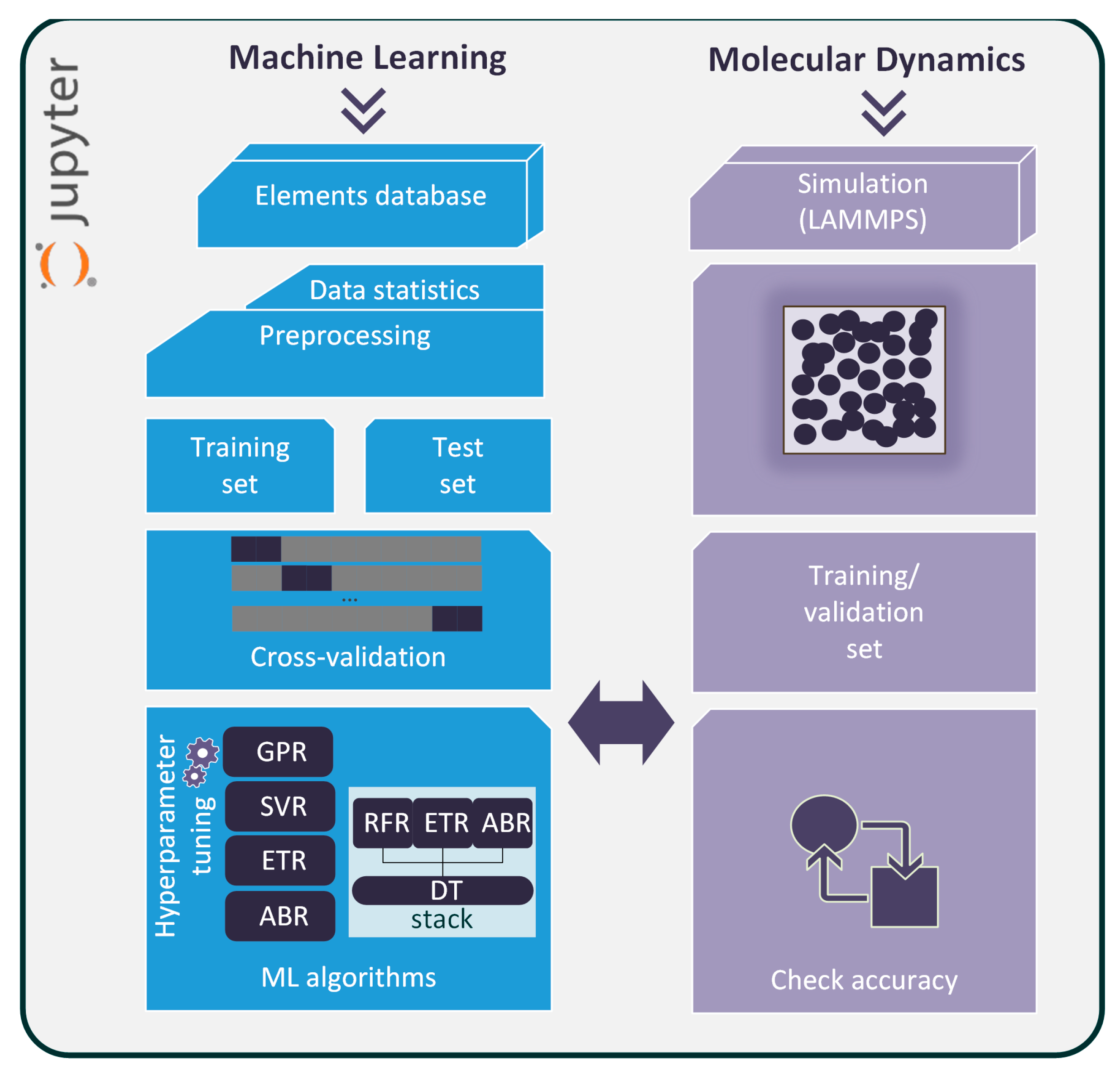
Therefore, it would be beneficial to embed novel ML methods into molecular simulations. In this paper, a combined MD simulation/ML prediction scheme has been constructed to accurately derive the transport properties, such as viscosity and thermal conductivity, of basic elements (argon, krypton, nitrogen, and oxygen) at the bulk state. The framework is embedded in a Jupyter Lab environment [16]. It starts by analyzing historical data from the literature [17], performs property prediction with available data, and functions in parallel to an MD computational flow that calculates the transport properties in phase space points where no data is available. The ML model is further fed with MD-extracted points, and it is then retrained, achieving increased accuracy in most cases. The fast ML platform is capable of extracting new phase-state points while remaining linked to the MD simulations, ensuring that results are accurate and bound to physical laws. Of equal importance is the enrichment of the data in the current literature with new values of viscosity and thermal conductivity which can be further processed by the research community.

2. Simulation Model and Data Analysis

2.1. Computational Framework

A flow diagram of the computational model constructed is given in Figure 1. Historical data from the literature [17], after being pre-processed and normalized, enters the computational platform to feed a series of ML algorithms. The available data is divided into a training dataset (80%) and a test dataset (20%) through a 10-fold cross-correlation technique that randomly assigns ten different portions of data to the categories of training and test data. In every iteration, a different portion of data is considered to be training (e.g., 8 out of 10) and test (e.g., the remaining 2 out of 10), which is a common practice used to minimize the possibility of overfitting [18].

To find the best-performing algorithm that fits in the transport properties dataset, a number of different ML algorithms have been tested in order to determine their accuracy, based on kernel, ensemble, and stack methods. In regression problems, it has been found that different algorithms achieve different metrics in scalability and predictive accuracy [19]. Here, the Gaussian Process Regressor (GPR), the Support Vector Regressor (SVR), the AdaBoost Regressor (ABR), and the Extra Trees Regressor (ETR) are employed. GPR and SVR are kernel-based methods, while ABR and ETR combine the decision-tree principle with an ensemble learning approach. Furthermore, a stack method, employing various algorithms in a stacked manner, has also been created. All algorithms are set after a hyperparameter tuning procedure which adjusts their parameters to the specific problem [20], which ensures that they run with the optimal parameters to achieve maximum accuracy [21]. The accuracy of the computational procedure is validated by comparing it to newly extracted EMD simulation data. The MD computational flow is executed in parallel in the open-source LAMMPS software [22]. New data coming from the MD flow enter the ML process to retrain and further validate the output.

More specifically, the calculations begin by feeding the initial elements database into the ML algorithm, and after the pre-processing stage, the algorithm is trained and validated on existing data through the cross-correlation pipeline. This process is repeated for each algorithm and for each element incorporated here. Next, the predictive accuracy of each algorithm is assessed through a computational loop. At this point, an MD simulation is established for a new phase space point (P-T) that does not exist in the initial database and the derived viscosity and thermal conductivity values are added to the database. The ML algorithm runs once more with the enriched database and its performance accuracy is tabulated. It becomes clear that the MD simulations provide new data for processing, at fluid states not reported in the literature, and, at the same time, an alternative ML model is trained on this data and is capable of predicting more state points in a future step, bypassing the MD simulations. This computation scheme exploits the accuracy of MD and combines it with the ML speed to suggest a twofold procedure that could be employed in similar property-prediction applications.

A major advantage of the proposed framework is the fact that all computational subsystems are controlled by a Jupyter Lab Python environment. This means that MD and ML codes communicate and can interact with each other, while data is available for processing and analysis at every stage of the process.

2.2. Data Description and Pre-Processing

The database of the elements used in our study [17] includes values for the viscosity (η) and thermal conductivity (λ) of argon (Ar), krypton (Kr), nitrogen (N), and oxygen (O). The data refer to (P-T) phase-state points, i.e., the obtained values for viscosity and thermal conductivity at specific (P-T) values. This means that the ML models implemented accept two inputs, P and T, and output η and λ. In the available database, viscosity data for Ar and N were obtained using experimental methods such as capillary flow (CF) and the oscillating disc (OD). Thermal conductivity data were acquired by techniques such as the parallel plate (PP) and concentric cylinder (CC) apparatuses. For Kr, the principle of corresponding states has been used to calculate the transport properties, while for O, limited data for thermal conductivity, compared to the other elements, is given due to challenges in obtaining reliable values, particularly at higher temperatures.

Data is provided for temperature (T), starting from the triple-point temperature up to 500 K, and for pressures to the value of P = 100 MPa. The (P-T) phase space for each element is presented in Figure 2. The critical and the triple points define the regions where phase changes occur, and have different values for each element. Data statistics are given in

Table 1. Element data statistics. Apart from the literature, phase-state points enhanced with MD have also been calculated and incorporated in the analysis made. Critical points for T (T_c) and P (P_c) are shown.

Element	η (μg/cm·s) [17]	λ (μW/(K·m)) [17]	η (μg/cm·s) (from MD)	λ (μW/(K·m)) (from MD)	T (K) Range	Tc (K)	P (MPa) Range	Pc (MPa)
Ar	1219	1259	200	200	86–500	150.68	0.1–100	4.86
Kr	506	506	30	5	125–500	209.41	0.1–20	5.5
N	1275	1253	20	40	75–500	126.20	0.1–100	3.39
O	814	814	18	14	75–500	154.60	0.1–35	5.04

. The amount of data provided from the literature is sufficient for application to an ML investigation, and the data will also be enriched by the MD we perform. The phase space covers the range from ambient gas and liquid conditions to extreme, at supercritical states. There is no investigation of solids in the present work.

Moreover, in order to check for possible correlations within the data, we also present, in Figure 3, correlation maps for each element. The inputs P and T are clearly not correlated for all elements. For Ar, a medium negative correlation is observed between T and both transport properties (Figure 3a,b). Krypton’s properties are mostly affected by temperature. Nitrogen’s properties are slightly correlated with those of T. On the other hand, the properties of O are strongly correlated only with those of T. In all cases, both thermal conductivity and viscosity present near-to-zero correlation with P.

Data is normalized in order to restrict the input value range and allow the ML algorithms to perform better, whereby a data point, $x$, transforms to

$$z=\frac{x-\overline{x}}{s},$$

(1)

where $\overline{x}$ is the mean value of the samples and $s$ the standard deviation.

2.3. Machine-Learning Algorithms

2.3.1. Support Vector Regression

Support vector regression is a variation of support vector machines (SVM) that is specifically tailored for regression analysis. SVR aims to find a regression function that maps input data points to continuous output values while maximizing the margin between the predicted values and a defined margin of error. This margin is controlled by two parameters: the error tolerance (epsilon, ε) and a regularization parameter (C) which balances the trade-off between achieving a smaller margin and minimizing prediction errors. The implementation of the technique is summarized in five steps:

• Data preparation: Input data is collected, including features (variables) and corresponding target values (continuous output).
• Feature scaling: It is essential to scale the features to ensure that they have similar ranges. Common scaling methods include normalization (scaling to [0, 1]) or standardization (mean = 0, variance = 1).
• Kernel selection: SVR uses kernels to map the data into a higher-dimensional space where it may be easier to find a linear separation. Common kernel functions include linear, polynomial, radial basis function (RBF), and sigmoid kernels.
• Model training: SVR aims to find a boundary window that has the maximum margin on both sides of the data points, while allowing some points to fall within a margin of error ε. The training process involves solving an optimization problem to determine the support vectors (data points that influence the margin) and the model parameters.
• Prediction: Once the SVR model is trained, it can predict the continuous output values for new unseen data points.

The SVR can be applied to various property estimation tasks in fluid mechanics, such as the determination of the minimum miscible pressure in modeling membrane separation systems, or the prediction of the pan evaporation in hydrological and ecological settings [23,24,25], to mention a few.

2.3.2. Gaussian Process Regression

Gaussian process regression is a non-parametric ML algorithm used for regression tasks. It uses probabilistic modeling to make predictions and provide uncertainty estimates based on training data. GPR assumes that the relationship between input features and outputs follows a Gaussian process distribution, which allows it to capture complex patterns and provide confidence intervals for predictions. The equation for GPR is expressed as

$$y=\mu +\epsilon ,$$

(2)

where y is the predicted output, µ is the mean of the Gaussian process distribution, and ε is the random noise term. This method also uses kernels (or covariance functions) to determine the shape and characteristics of the Gaussian process distribution. Common kernel functions include both the Matèrn and exponential forms of the radial basis function (RBF). The choice of kernel function influences how the GPR model captures correlations between data points. Here, we have applied a Matèrn kernel, which is common choice in the applied sciences and in engineering [26,27]. The algorithm has hyperparameters that need to be tuned, such as the parameters of the kernel function and the noise level. Properly tuning these hyperparameters is essential for the model’s performance and for its ability to capture the underlying patterns in the data [28,29,30].

GPR not only provides point predictions but also estimates the uncertainty associated with each prediction. It computes prediction intervals that indicate the range within which the true output is likely to fall. This is particularly useful in fluid mechanics applications, for which understanding the uncertainty of predictions can be crucial. Examples of applications include property predictions such as fluid flow rate, pressure distribution, and heat-transfer coefficients. GPR has also the advantage of dealing with limited and noisy data effectively by further quantifying the uncertainty inside the predictions [31,32,33].

2.3.3. The Extra Trees Regressor

The Extra Trees Regressor is an ensemble learning algorithm that belongs to the family of decision tree algorithms, functioning as an extension of the Random Forest (RF) algorithm [34]. ETR builds multiple decision trees and combines their predictions to provide more robust and accurate results. Each decision tree predicts the target variable for a given input, and the final prediction is a combination of predictions from all trees. However, unlike RF, the ETR does not consider bootstrap sampling, and it selects random features at each split point without using any specific criteria. Equation (3) can express the general prediction equation for the Extra Trees Regressor:

$$\widehat{y}=\frac{1}{N}{\sum }_{i=1}^N{f}_i\left(X\right),$$

(3)

where $\widehat{y}$ is the predicted target value, N is the total number of decision trees in the ensemble, and $f_i\left(X\right)$ is the prediction of the ith decision tree for the input X. The randomness introduced during the tree-building process can reduce overfitting. Additionally, the ETR is computationally efficient due to its parallelism in training multiple trees. However, it is essential to note that the choice of hyperparameters, such as the number of trees and their maximum depth, can impact the algorithm’s performance. Cross-validation is also important here. In fluid mechanics applications, ETR has been employed to predict various fluid-related properties, such as molecular separation in membrane systems, Vibrio fischeri toxicities, properties of ionic liquid, ink droplet velocity profiles of printing cells, and drug particle solubility optimization [10,35,36,37,38].

2.3.4. AdaBoost Regressor

The AdaBoost Regressor combines the predictions of multiple weak learners, often decision trees, to create a strong ensemble model. The final prediction is a weighted average of the predictions made by each weak learner. The general prediction equation can be expressed by

$$\widehat{y}={\sum }_{i=1}^N{w_{i}f}_i\left(X\right),$$

(4)

where $\widehat{y}$ is the predicted target value, N is the total number of weak learners in the ensemble, w_i is the weight assigned to the prediction of the ith weak learner, and $f_i\left(X\right)$ is the prediction of the ith weak learner for the input X. In each iteration, the weights of misclassified instances are increased, forcing the algorithm to focus more on those instances. The weak learners are trained sequentially, with each one adjusting its predictions based on the weighted errors of the previous iterations. ABR is particularly useful when dealing with complex relationships in data, capturing non-linear patterns. It is effective in reducing bias and improving the overall accuracy of predictions. However, it can be sensitive to noisy data and outliers, as these can negatively impact the performance of weak learners. In fluid mechanics applications, AdaBoost Regressor has been successfully employed to predict fluid flow rates, pressure drop, concentration in water purification via porous membranes, droplet volume in printing technologies, and biodiesel yield and viscosity [39,40,41,42].

2.3.5. Stacked Models

Stacking, also known as stacked generalization, is an ML ensemble algorithm that combines multiple models (learners) to create a more accurate and robust predictive model. The basic mechanism behind stacking is to train several diverse base models and then use a meta-model to combine their predictions to make the final prediction. The stacking algorithm involves two main steps: training base models and training a meta-model. For stacking, multiple base models are trained on the same dataset. Each base model generates predictions for the target variable based on the input features. The predictions from these base models are then used as features for the next step. A meta-model, also known as a blending or aggregator model, is trained using predictions generated by the base models as features. The target variable is the same as the original target variable. The meta-model learns how to weigh or combine the predictions of the base models to produce the final prediction,

$${\widehat{y}}_{final}=MetaModel\left({\widehat{y}}_{base1},{\widehat{y}}_{base1},\dots , {\widehat{y}}_{baseN}\right),$$

(5)

where ${\widehat{y}}_{final}$ is the final predicted target value, ${\widehat{y}}_{basei}$ is the predicted target value from the ith base model, and MetaModel is the function that combines the predictions of the base models. Stacking is powerful because it leverages the diversity of predictions from multiple models. By combining the strengths of different models, it can achieve higher predictive accuracy than individual models. However, it can be computationally intensive and may require thoughtful tuning to avoid overfitting. In fluid mechanics applications, stacking can be used to predict various fluid properties, like flows in membranes. Soil industry, seismology, and geophysics have been the major utilizers of this method [43,44,45,46,47,48].

In this paper, we have employed the predictive power of ensemble, tree-based algorithms to create the stacked model. More specifically, the ABR, ETR, and Random Forest (RFR) algorithms have been used for calculations, and their outcomes are combined by Decision Trees (DT) algorithm. A general flowchart is embedded in the ML side of Figure 1.

2.4. Molecular Dynamics Model

Molecular Dynamics (MD) simulation is a computational technique widely used to investigate the behavior of systems at the atomic level [49,50,51]. For our calculations, we have employed the LAMMPS software to simulate the elements at the bulk state. The Lennard-Jones (LJ) potential is considered for the construction of the system’s inter-relations and the output of the simulation provides the two important thermophysical properties, viscosity and thermal conductivity, η = f (P, T) and λ = f (P, T), respectively, through a wide range of pressure (P) and temperature (T) values.

The 12-6 LJ potential is given by

$$u_{LJ}=4\epsilon \left[{\left(\frac{\sigma }{r_{ij}}\right)}^{12}-{\left(\frac{\sigma }{r_{ij}}\right)}^6\right],$$

(6)

with a cut-off radius r_c = 2.5σ. The values of the LJ parameters σ and ε and the masses of the particles, m, are presented in

Table 2. LJ parameters of the elements incorporated in the MD simulations.

Element	$\mathit{ϵ}$/k (K)	σ (nm)	m (a.u.)
Argon (Ar)	152.8	3.297	39.948
Krypton (Kr)	215.8	3.513	83.798
Nitrogen (N)	118.0	3.54	14.0067
Oxygen (O)	113.0	3.437	15.999

.

The simulation box that encloses the bulk fluids is a cube with dimensions $\left(10\times 10\times 10\right)$ LJ units (σ) in the x, y, and z directions. Fluid particles are initially placed in a face-centered cubic (fcc) lattice and left to attain their final positions through an initialization stage. After an equilibration phase of 10⁶ MD timesteps (the timestep is Δt = 1 fs), in which temperature and pressure stabilize at constant values, the system reaches the stable state and parallel production runs (at least 10 for every case, for statistical accuracy) begin for 10⁷ MD steps. Fluid density, pressure and temperature are the properties that control the simulations. Different combinations produce new values for our MD database. Simulations evolve through the NPT (Isothermal-Isochoric) ensemble, with a Nose–Hoover thermostat used to control the fluid temperature and a barostat used to control the pressure [52,53,54,55,56].

2.4.1. Thermal Conductivity Calculation

The heat flux is calculated for each atom in the system. In an fcc lattice, the heat flux vectors represent heat flow along the face diagonals of the cubic cells. Heat flux quantifies the rate at which heat energy is transferred through the system. It is computed for each particle by considering the particle’s kinetic energy, potential energy, and stress contributions. It is a vector quantity, representing heat flow along each Cartesian direction (x, y, z), with components defined as ‘J_x’, ‘J_y’, and ‘J_z’. The ‘fix ave/correlate’ LAMMPS command is used to calculate the correlation of the heat flux components over time, and the correlation function is then integrated to obtain the thermal conductivity components λ_xx, λ_yy, and λ_zz.

The heat flux J_x(t) in the x-direction for each atom is computed using Equation (7), as

$${\mathrm{J}}_x\left(\mathrm{t}\right)=\frac{\mathrm{K}\mathrm{E}\left(\mathrm{t}\right)}{\mathrm{V}}+\frac{\mathrm{P}\mathrm{E}\left(\mathrm{t}\right)}{\mathrm{V}}+\frac{\mathsf{\sigma }\mathrm{x}\mathrm{x}\left(\mathrm{t}\right)}{\mathrm{V}},$$

(7)

where KE(t) and PE(t) are the kinetic and potential energies, respectively, and σ_xx(t) is the stress tensor component along the x-direction. The Green–Kubo (GK) method is employed to calculate the thermal conductivity λ, as

$$\lambda =\frac{{Vk}_B}{3}{\int }_0^{\infty }〈J_x\left(t\right)·J_x\left(0\right)〉dt,$$

(8)

with V as the system volume and k_B the Boltzmann’s constant [57,58].

2.4.2. Viscosity Calculation

Viscosity characterizes a fluid’s resistance to flow. In this MD model, viscosity, η, is calculated using the GK method from the components of the stress tensor ${\sigma }_{xy}$ [59], in a manner similar to thermal conductivity, as

$$\eta =\frac{V}{k_{B}T}{\int }_0^{\infty }〈{\sigma }_{xy}\left(t\right)·{\sigma }_{xy}\left(0\right)〉dt.$$

(9)

The stress velocity correlation function in Equation (9) is calculated to determine how the stress (pressure) influences the fluid’s flow behavior,

$$〈{\sigma }_{xy}\left(t\right)·{\sigma }_{xy}\left(0\right)〉.$$

(10)

3. Results and Discussion

With a series of parallel MD simulations, viscosity and thermal conductivity values for (P-T) state points missing from the elements database have been calculated. We have to note here that the base MD program has been verified on the specific database values. To validate the results of the simulations, we first calculated the values of η and λ provided in the database (i.e., the existing data points), for which we have taken the same or nearly the same values, within statistical accuracy, and next, we proceeded to calculate the unknown data points.

Next, characteristic algorithmic implementations concerning the MD code were described; all calculated transport properties values are given in the respective Tables. All of this data is embedded in the initial elements database and the predictive ability of our ML algorithms is evaluated.

3.1. MD Programming

Both thermal conductivity and viscosity components are reported as running averages over the whole simulation time [60]. Due to the sophisticated computational techniques needed to automatically extract MD-calculated values for viscosity and thermal conductivity, a hypercomputer system (HPC) has been deployed. Computational techniques incorporated to manage data files for each element, for every (P-T) pair and for every simulation instance (as discussed above, we have performed 10 parallel simulations to extract one average value for statistical reasons), are embedded in a Jupyter Lab Python environment.

First, we prepare the input files and place them in separate folders for each available case that runs on LAMMPS, and for each element (4 elements), temperature (20 different temperature values), and pressure (10 different pressure values) range. This is performed automatically for the $(4\times 20\times 10)=800$ simulation instances; the procedure is shown in Algorithm 1.

Algorithm 1. Prepare and run MD simulations
1:	Open generic LAMMPS bulk fluid simulation file
2:	Define element masses list, m = [·]
3:	Create file path for every element
4:	Define temperature range list, T = [·]
5:	Create file path for every temperature value
6:	Define pressure range list, P = [·]
7:	Create file path for every pressure value
8:	for i, j, k in mi = [·], Tj = [·], Pk = [·]
9:	Create LAMMPS input files

Algorithm 2 depicts the MD program flow in LAMMPS. After proper initialization, the code runs in 10 parallel instances to achieve better statistical accuracy and calculates the properties of interest. This is performed for every case constructed by Algorithm 1. In the final stage of a simulation, calculated values for viscosity and thermal conductivity are stored in a Pandas DataFrame and, finally, in .csv files. All values are embedded in the initial elements database.

Algorithm 2. Backbone of a bulk fluid MD simulation
1:	Define simulation box, units, atom_style
2:	Setup simulation variables (P, T, ρ, rc, lattice constant)
3:	Setup LAMMPS computes: temperature and pressure
4:	Initialization run for t = 106 timesteps
5:	Give random initial velocity values to particles
6:	Define pair styles and pair coefficients
7:	Begin NPT simulation
8:	for i = 1:10
9:	ith production run:
10:	Calculate kinetic and potential energy per atom
11:	Calculate stress tensors and heat flux components
12:	Perform time auto-correlations
13:	Calculate pair correlation function
14:	Calculate viscosity and thermal conductivity
15:	Statistical averaging of the results
16	Store calculated values to pandas dataframe
17:	Store calculated values to .csv in the respective folder

3.2. MD Simulations

Turning our attention to the transport properties extracted from the MD simulations now, we present calculated viscosity and thermal conductivity values for Ar in

Table 3. MD-extracted Ar viscosity values, in (μg/cm$·$s).

P, MPa T, K	2.5	3	3.5	4	4.5	5	5.5	6	6.5	7
122	915.92	898.93	984.93	1031.25	918.71	966.45	1073.30	999.74	1038.84	1056.03
127	856.09	870.47	846.76	902.07	825.29	885.12	822.00	840.84	991.45	899.43
132	739.48	668.68	712.28	738.41	772.78	722.18	743.04	761.02	703.95	848.49
137	560.58	597.45	601.79	659.04	585.75	664.99	651.53	660.57	702.26	693.07
142	117.64	147.14	86.62	481.58	487.14	555.57	580.50	604.51	632.08	643.75
147	126.46	122.85	136.91	141.95	177.16	426.69	464.30	477.40	504.92	570.44
152	136.84	140.36	138.27	150.60	172.48	179.28	229.33	318.64	405.40	432.61
157	146.23	144.80	158.39	152.49	153.81	174.39	181.17	216.45	229.40	328.56
162	146.32	148.01	155.79	151.34	162.92	143.66	185.92	193.01	205.05	222.15
167	144.75	151.00	142.66	150.15	174.37	157.78	168.46	190.36	196.99	202.15
172	154.98	138.00	149.39	162.98	162.99	178.80	186.19	191.40	192.16	196.04
177	155.70	160.01	157.61	163.30	155.16	187.89	192.83	184.26	197.63	205.62
182	162.06	151.75	174.93	177.68	191.47	185.64	177.72	180.83	199.93	185.79
187	146.68	151.42	177.72	172.29	171.85	185.45	191.96	187.61	198.33	229.21
192	162.91	173.95	173.98	190.22	172.68	184.91	177.29	187.52	208.48	193.12
197	163.13	164.06	164.92	185.37	165.11	169.06	168.62	184.49	184.17	191.25
202	181.09	183.14	190.11	175.38	180.24	181.74	188.42	184.45	200.43	208.96
207	173.99	190.19	185.76	181.99	183.47	170.59	198.19	210.16	178.74	220.90
212	160.56	165.03	193.46	192.82	201.60	223.12	175.56	202.08	205.86	217.05
217	177.43	183.18	179.69	198.42	183.86	189.87	198.23	205.96	191.67	194.21

and

Table 4. MD-extracted Ar thermal conductivity values, in (μW/(K$·$m).

P, MPa T, K	2.5	3	3.5	4	4.5	5	5.5	6	6.5	7
122	73.01	75.49	75.33	80.60	75.38	80.08	79.08	81.27	80.28	76.70
127	70.15	71.65	69.81	70.66	68.74	75.77	68.74	76.76	72.10	79.16
132	60.03	54.50	64.09	61.41	66.34	64.24	66.48	67.14	68.02	68.29
137	55.45	56.01	55.10	54.23	58.52	62.14	63.14	59.00	64.63	60.67
142	11.67	13.90	41.27	45.68	44.05	49.00	56.23	55.53	51.21	54.05
147	12.15	13.38	14.27	17.60	25.02	43.41	41.95	47.16	48.43	47.37
152	10.60	13.16	13.59	14.24	15.50	18.73	27.72	37.90	42.08	42.11
157	11.79	13.52	11.81	14.62	15.62	17.45	21.61	24.00	28.83	31.95
162	11.09	12.87	13.66	15.46	16.29	15.85	18.25	20.91	23.91	26.93
167	11.33	12.33	12.41	13.80	14.55	17.83	16.66	18.88	23.75	22.84
172	11.31	12.04	14.30	14.84	14.97	16.51	15.68	18.25	19.41	22.22
177	12.83	13.69	12.74	13.01	14.54	15.99	13.68	18.77	18.71	18.90
182	13.25	13.60	13.36	13.72	14.70	16.79	15.49	17.32	18.46	19.23
187	12.23	12.72	13.80	14.91	15.73	15.95	16.18	17.75	18.02	16.17
192	12.50	13.32	14.78	13.14	15.07	15.02	15.34	16.42	17.57	19.08
197	12.25	13.18	14.29	14.67	15.63	15.92	18.09	18.02	18.31	16.61
202	12.65	11.92	14.41	15.18	15.43	16.39	16.80	16.39	19.76	17.96
207	12.26	12.18	13.90	14.91	14.45	17.36	15.49	17.00	17.20	19.44
212	13.41	13.86	14.22	14.74	15.62	17.12	17.11	17.27	18.23	19.74
217	13.09	14.85	14.30	14.23	16.53	15.45	16.87	17.78	19.61	19.38

, for Kr in

Table 5. MD-extracted Kr viscosity values, in (μg/cm$·$s).

T, K	P, MPa	$\mathit{\eta }, \mathsf{\mu }\mathbf{g}/\mathbf{cm}·$s	T, K	P, MPa	$\mathit{\eta }, \mathsf{\mu }\mathbf{g}/\mathbf{cm}·$s
177	0.5	157.74	152	6.0	2485.56
212	0.5	186.81	162	6.0	2143.70
152	1.0	2184.46	177	6.0	1647.74
157	1.0	1998.47	187	6.0	1314.75
162	1.0	171.38	192	6.0	1183.46
207	1.0	185.60	197	6.0	1151.88
147	2.0	2579.93	202	6.0	982.18
157	2.0	2136.94	207	6.0	830.09
162	2.0	1881.72	212	6.0	590.38
177	2.0	182.64	217	6.0	351.66
147	4.0	2511.72	162	10.0	2190.60
167	4.0	1868.86	167	10.0	2004.87
187	4.0	1223.95	172	10.0	1814.65
202	4.0	386.81	182	10.0	1548.39
217	4.0	223.73	197	10.0	1213.54

and

Table 6. MD-extracted Kr thermal conductivity values, in (μW/(K$·$m).

T, K	P, MPa	$\mathsf{\lambda }, \mathsf{\mu }\mathbf{W}/(\mathbf{K}·$m)
122	2.0	96.48
127	2.0	90.52
137	2.0	82.57
147	2.0	75.04
152	2.0	72.04

, for N in

Table 7. MD-extracted N viscosity values, in (μg/cm$·$s).

T, K	P, MPa	$\mathit{\eta }, \mathsf{\mu }\mathbf{g}/\mathbf{cm}·$s	T, K	P, MPa	$\mathit{\eta }, \mathsf{\mu }\mathbf{g}/\mathbf{cm}·$s
122	0.1	82.73	127	4.0	188.13
122	0.5	84.40	132	4.0	158.94
132	1.5	95.71	137	4.0	124.86
142	1.5	100.94	152	4.0	123.76
147	1.5	105.32	132	5.0	196.40
122	2.0	95.71	152	5.0	135.21
157	2.5	115.14	137	6.0	227.88
122	3.0	120.58	142	6.0	176.06
137	3.0	110.32	147	6.0	165.24
127	3.5	137.57	217	6.0	157.40

and

Table 8. MD-extracted N thermal conductivity values, in (μW/(K$·$m).

T, K	P, MPa	$\mathsf{\lambda }, \mathsf{\mu }\mathbf{W}/(\mathbf{K}·$m)	T, K	P, MPa	$\mathsf{\lambda }, \mathsf{\mu }\mathbf{W}/(\mathbf{K}·$m)
122	2.5	19.88	157	5	24.40
127	2.5	18.98	187	5	23.27
157	2.5	19.37	217	5	24.42
192	2.5	20.25	132	6	60.90
197	2.5	20.95	137	6	49.37
207	2.5	21.24	152	6	30.34
127	3	24.18	217	6	25.43
132	3	20.55	137	7	56.31
192	3	20.90	142	7	44.29
207	3	21.78	157	7	32.55
142	3.5	23.66	167	7	28.00
182	3.5	21.14	172	7	27.51
192	3.5	21.43	182	7	26.56
132	4	33.04	187	7	26.39
137	4	27.81	217	7	26.47
147	4	22.42	132	8	57.70
192	4	22.08	142	8	49.84
127	5	48.07	152	8	37.44
142	5	32.75	157	8	34.85
152	5	26.26	182	8	28.34

, and for O in

Table 9. MD-extracted O viscosity values, in (μg/cm$·$s).

T, K	P, MPa	$\mathit{\eta }, \mathsf{\mu }\mathbf{g}/\mathbf{cm}·$s	T, K	P, MPa	$\mathit{\eta }, \mathsf{\mu }\mathbf{g}/\mathbf{cm}·$s
132	1.0	101.48	137	2.0	112.02
137	1.0	106.91	152	2.0	121.22
147	1.0	112.02	162	2.0	127.15
157	1.0	121.22	167	2.0	130.26
172	1.0	130.26	142	2.5	118.88
127	1.5	100.63	142	3.0	124.90
142	1.5	112.02	147	3.0	126.80
157	1.5	122.00	152	3.0	128.88
162	1.5	129.85	147	3.5	128.59

and

Table 10. MD-extracted O thermal conductivity values, in (μW/(K$·$m).

T, K	P, MPa	$\mathsf{\lambda }, \mathsf{\mu }\mathbf{W}/(\mathbf{K}·$m)	T, K	P, MPa	$\mathsf{\lambda }, \mathsf{\mu }\mathbf{W}/(\mathbf{K}·$m)
207	0.1	19.09	172	5	25.94
212	0.1	19.65	177	5	25.23
217	0.1	19.94	192	5	24.11
127	1.5	27.39	182	6	27.39
152	4	26.74	187	6	26.74
157	4	25.23	192	6	25.94
162	4	23.89	197	6	25.74

, respectively. These values are embedded in the initial property database (taken from the literature) and employed for transport property prediction in the ML model constructed. We have to note that tabulated values shown here are taken far from the critical points, and their values are close to neighboring, validated results found in the literature-only database.

The initial database for Kr is significantly smaller compared to that for Ar (see Table 1). The Kr MD simulations have given many outlier values; in order to ensure that our ML model performs in an equally fine manner, we have kept only the simulation values close to neighboring ones. Also, a similar strategy has been followed for the N and O elements.

3.3. Machine-Learning Predictions

The ability of the implied ML algorithms to predict the transport properties of the elements is captured by the accuracy measures shown in

Table 11. Metrics of accuracy for viscosity (η) and thermal conductivity (λ) coefficients, as achieved by each ML algorithm, for the initial database.

		Ar		Kr		N		O
		η	λ	η	λ	η	λ	η	λ
SVR	ΜAΕ	17.73	1.33	68.19	0.94	9.89	1.49	24.69	2.15
	RMSE	69.41	4.01	292.16	4.08	41.07	7.87	83.94	7.36
	MAPE	0.09	0.05	0.38	0.08	0.07	0.04	0.13	0.08
	R2	0.99	0.99	0.95	0.98	0.99	0.97	0.99	0.98
GPR	ΜAΕ	27.22	2.76	55.15	1.45	19.30	2.14	33.43	3.48
	RMSE	68.49	6.65	182.73	4.49	77.77	7.89	136.80	10.12
	MAPE	0.08	0.07	0.19	0.13	0.07	0.04	0.11	0.09
	R2	0.99	0.98	0.98	0.98	0.95	0.97	0.97	0.97
ABR	ΜAΕ	19.93	1.46	39.57	1.47	12.33	2.00	27.08	1.91
	RMSE	84.54	4.79	72.67	6.39	50.62	8.61	99.60	9.05
	MAPE	0.09	0.05	0.04	0.13	0.07	0.06	0.10	0.05
	R2	0.98	0.98	0.99	0.97	0.98	0.96	0.98	0.98
ETR	ΜAΕ	10.20	1.03	41.75	0.80	8.3	1.24	14.28	1.15
	RMSE	56.68	3.36	201.33	3.17	47.14	7.05	63.80	5.92
	MAPE	0.06	0.04	0.22	0.09	0.05	0.04	0.08	0.06
	R2	0.99	0.99	0.98	0.99	0.98	0.98	0.99	0.99
SA	ΜAΕ	12.38	1.01	48.25	1.09	9.33	0.98	13.29	0.88
	RMSE	61.96	2.87	205.11	4.03	44.80	4.18	50.49	3.38
	MAPE	0.06	0.04	0.20	0.07	0.05	0.04	0.06	0.03
	R2	0.99	0.99	0.98	0.99	0.98	0.99	0.99	0.99

. The mean absolute error (MAE) is given by

$$MAE=\frac{1}{n}{\sum }_{i=1}^n\left|Y_i\right|,$$

(11)

where $Y_i=y_{real,i}^{\mathrm{*}}-y_{pred,i}^{\mathrm{*}}$ for the ith data point; index real, the database value; pred, the ML predicted value.

The root mean squared error (RMSE) is

$$RMSE=\sqrt{{\sum }_{i=1}^n\frac{{\left(Y_i\right)}^2}{n}},$$

(12)

the mean absolute percentage error (MAPE) is

$$MAPE=\frac{1}{n}\sum _{i=1}^n\left|\frac{Y_i}{y_{exp,i}^{\mathrm{*}}}\right|,$$

(13)

and, finally, the coefficient of determination, R², is given by

$$R^2=1-\frac{{\sum }_{i=1}^N{\left(y_{real.,i}^{\mathrm{*}}-{\overline{y}}_{real.}^{\mathrm{*}}\right)}^2}{{\sum }_{i=1}^N{\left(Y_i\right)}^2}.$$

(14)

In Table 11, only the initial database (without MD-extracted values) has been considered for the calculations. In general, the algorithms incorporated here are capable of providing accurate predictions for all element-transport properties. As expected, the stacked algorithm (SA) has given the most accurate results for all elements. However, the ETR has given almost similar and in some cases, even more accurate results than SA. The algorithms that exploit kernels, such as SVR and GPR, are also good choices, although there may be some increased computational cost, as compared to the tree-based algorithms. Nevertheless, this overhead is not important in small and medium-sized datasets, such as the one that has been incorporated into this paper.

Furthermore, the initial database contains Kr values that have been calculated based on the principle of the corresponding states [61]. This is an indirect method used to obtain the properties of the elements, but we do not expect it to be of the same accuracy as an experimental or a proper simulation technique. Taking also into consideration that the Kr data points only number 516 (see Table 1), we believe that these are the two reasons why the accuracy measures for Kr are smaller, as compared to all other elements.

In

Table 12. Metrics of accuracy for viscosity (η) and thermal conductivity (λ) coefficients, as achieved by each ML algorithm, for the initial database with the addition of new MD-calculated data.

		Ar		Kr		N		O
		η	λ	η	λ	η	λ	η	λ
SVR	ΜAΕ	20.24	1.35	69.20	1.16	6.92	1.17	37.63	2.80
	RMSE	58.84	4.03	255.79	4.44	28.04	5.15	128.81	12.41
	MAPE	0.06	0.05	0.33	0.09	0.04	0.04	0.20	0.08
	R2	0.99	0.99	0.95	0.98	0.99	0.99	0.98	0.96
GPR	ΜAΕ	42.11	3.12	57.24	1.53	17.34	2.06	50.39	3.22
	RMSE	128.80	8.71	186.75	4.56	58.04	5.28	135.68	11.65
	MAPE	0.08	0.08	0.16	0.13	0.04	0.05	0.23	0.06
	R2	0.97	0.96	0.97	0.98	0.98	0.99	0.98	0.97
ABR	ΜAΕ	18.68	1.38	27.10	1.33	3.69	1.53	22.89	2.77
	RMSE	54.57	4.64	52.32	6.11	27.92	6.68	71.20	13.07
	MAPE	0.04	0.05	0.03	0.12	0.02	0.05	0.09	0.04
	R2	0.99	0.99	0.99	0.97	0.99	0.97	0.99	0.96
ETR	ΜAΕ	15.21	0.96	27.06	1.33	9.10	1.53	22.89	2.77
	RMSE	66.62	3.28	52.32	6.11	27.92	6.68	71.20	13.70
	MAPE	0.04	0.04	0.03	0.12	0.02	0.05	0.09	0.04
	R2	0.99	0.99	0.99	0.97	0.99	0.98	0.99	0.96
SA	ΜAΕ	17.38	0.83	46.91	1.05	6.47	0.86	13.41	2.09
	RMSE	76.91	2.62	172.13	4.51	32.16	3.90	35.01	8.53
	MAPE	0.05	0.02	0.16	0.09	0.02	0.04	0.05	0.07
	R2	0.99	0.99	0.98	0.99	0.99	0.99	0.99	0.99

, the MD viscosity and thermal conductivity data have also been employed in the training and validation process, and every ML algorithm has been retrained. The accuracy of each algorithm is similar to those shown in Table 11, but some error metrics here have slightly increased. This deviation is small; it falls within the range of statistical accuracy. The new MD data points may be considered accurate, but, on the other hand, they come from a different method, computational—not experimental, and this may cause a kind of deviation from the real values. In any case, the deviations are small for Ar and N, and they increase a small amount more for O and Kr.

4. Conclusions

The transport properties of Ar, Kr, N, and O are examined in this paper. The main objectives are to calculate and predict viscosity and thermal conductivity. Experimental and theoretical data from the literature, after being pre-processed, has been initially exploited to train various machine-learning algorithms.

Ensemble, classical, kernel-based, and stacked algorithmic techniques have been proven effective in predicting the transport properties of fluid elements, achieving high levels of accuracy and low levels of error. Notwithstanding their performance, we have shown that they can be used in parallel with classical molecular dynamics simulations, in a twofold framework capable of exchanging information between the atomistic simulation and the machine-learning statistical backbone. The molecular dynamics framework incorporated is capable of producing training data automatically over a broad range of simulation conditions. Taking also into consideration that the observed accuracy of the developed machine-learning methods is enhanced, we expect that this twofold computational model will lead to substantial improvements in simulation applications, where possible.

This could open new directions in dealing with and calculating material properties. In cases where molecular dynamics (or another material-focused method’s) simulations are too time-consuming or expensive, machine learning can be incorporated as a faster and cost-effective alternative. Therefore, we believe that the bulk element simulation presented here can be upscaled in the future to deal with more complex fluids and confined geometries, even within wide ranges of temperatures and pressure conditions.

While the purpose of machine learning is not to create new physics, machine learning can be exploited to accelerate traditional computational methods. The future challenge is to become more interpretable, transparent, and explainable. This will allow scientists to better understand how the models work, and it will make these processes easier to apply in new and innovative ways. Incorporating machine learning into the field of fluid mechanics still has much to offer, and there is great potential for this technology to revolutionize the way that fluids are studied, modeled, and manufactured.

References

1. Allers, J.P.; Garzon, F.H.; Alam, T.M. Artificial Neural Network Prediction of Self-Diffusion in Pure Compounds over Multiple Phase Regimes. Phys. Chem. Chem. Phys. 2021, 23, 4615–4623. [Google Scholar] [CrossRef] [PubMed]
2. Desgranges, C.; Delhommelle, J. Towards a Machine Learned Thermodynamics: Exploration of Free Energy Landscapes in Molecular Fluids, Biological Systems and for Gas Storage and Separation in Metal–Organic Frameworks. Mol. Syst. Des. Eng. 2021, 6, 52–65. [Google Scholar] [CrossRef]
3. Yang, B.; Zhu, X.; Wei, B.; Liu, M.; Li, Y.; Lv, Z.; Wang, F. Computer Vision and Machine Learning Methods for Heat Transfer and Fluid Flow in Complex Structural Microchannels: A Review. Energies 2023, 16, 1500. [Google Scholar] [CrossRef]
4. Sofos, F.; Charakopoulos, A.; Papastamatiou, K.; Karakasidis, T.E. A Combined Clustering/Symbolic Regression Framework for Fluid Property Prediction. Phys. Fluids 2022, 34, 062004. [Google Scholar] [CrossRef]
5. Sanjuán, E.L.; Parra, M.I.; Pizarro, M.M. Development of Models for Surface Tension of Alcohols through Symbolic Regression. J. Mol. Liq. 2020, 298, 111971. [Google Scholar] [CrossRef]
6. El Hasadi, Y.M.F.; Padding, J.T. Solving Fluid Flow Problems Using Semi-Supervised Symbolic Regression on Sparse Data. AIP Adv. 2019, 9, 115218. [Google Scholar] [CrossRef]
7. Brunton, S.L.; Noack, B.R.; Koumoutsakos, P. Machine Learning for Fluid Mechanics. Annu. Rev. Fluid Mech. 2020, 52, 477–508. [Google Scholar] [CrossRef]
8. Garnier, P.; Viquerat, J.; Rabault, J.; Larcher, A.; Kuhnle, A.; Hachem, E. A Review on Deep Reinforcement Learning for Fluid Mechanics. Comput. Fluids 2021, 225, 104973. [Google Scholar] [CrossRef]
9. Stergiou, K.; Ntakolia, C.; Varytis, P.; Koumoulos, E.; Karlsson, P.; Moustakidis, S. Enhancing Property Prediction and Process Optimization in Building Materials through Machine Learning: A Review. Comput. Mater. Sci. 2023, 220, 112031. [Google Scholar] [CrossRef]
10. Sagi, O.; Rokach, L. Ensemble Learning: A Survey. WIREs Data Min. Knowl. Discov. 2018, 8, e1249. [Google Scholar] [CrossRef]
11. Drikakis, D.; Sofos, F. Can Artificial Intelligence Accelerate Fluid Mechanics Research? Fluids 2023, 8, 212. [Google Scholar] [CrossRef]
12. Callaham, J.L.; Maeda, K.; Brunton, S.L. Robust Flow Reconstruction from Limited Measurements via Sparse Representation. Phys. Rev. Fluids 2019, 4, 103907. [Google Scholar] [CrossRef]
13. Jirasek, F.; Hasse, H. Perspective: Machine Learning of Thermophysical Properties. Fluid Phase Equilibria 2021, 549, 113206. [Google Scholar] [CrossRef]
14. Karniadakis, G.; Beşkök, A.; Aluru, N. Microflows and Nanoflows: Fundamentals and Simulation; Springer: Berlin/Heidelberg, Germany, 2005; ISBN 978-0-387-22197-7. [Google Scholar]
15. Agarwal, A.; Arya, V.; Golani, B.; Bakli, C.; Chakraborty, S. Mapping Fluid Structuration to Flow Enhancement in Nanofluidic Channels. J. Chem. Phys. 2023, 158, 214701. [Google Scholar] [CrossRef] [PubMed]
16. Kluyver, T.; Ragan-Kelley, B.; Perez, F.; Granger, B.; Bussonnier, M.; Frederic, J.; Kelley, K.; Hamrick, J.; Grout, J.; Corlay, S.; et al. Jupyter Notebooks—A Publishing Format for Reproducible Computational Workflows. In Positioning and Power in Academic Publishing: Players, Agents and Agendas; IOS Press: Amsterdam, The Netherlands, 2016; pp. 87–90. [Google Scholar]
17. Hanley, H.J.M.; McCarty, R.D.; Haynes, W.M. The Viscosity and Thermal Conductivity Coefficients for Dense Gaseous and Liquid Argon, Krypton, Xenon, Nitrogen, and Oxygen. J. Phys. Chem. Ref. Data 1974, 3, 979–1017. [Google Scholar] [CrossRef]
18. Mendez, M.A.; Ianiro, A.; Noack, B.R.; Brunton, S.L. (Eds.) Data-Driven Fluid Mechanics: Combining First Principles and Machine Learning; Cambridge University Press: Cambridge, UK, 2023; ISBN 978-1-108-84214-3. [Google Scholar]
19. Huang, J.-C.; Ko, K.-M.; Shu, M.-H.; Hsu, B.-M. Application and Comparison of Several Machine Learning Algorithms and Their Integration Models in Regression Problems. Neural Comput. Applic. 2020, 32, 5461–5469. [Google Scholar] [CrossRef]
20. Yang, L.; Shami, A. On Hyperparameter Optimization of Machine Learning Algorithms: Theory and Practice. Neurocomputing 2020, 415, 295–316. [Google Scholar] [CrossRef]
21. Shahhosseini, M.; Hu, G.; Pham, H. Optimizing Ensemble Weights and Hyperparameters of Machine Learning Models for Regression Problems. Mach. Learn. Appl. 2022, 7, 100251. [Google Scholar] [CrossRef]
22. Plimpton, S. Fast Parallel Algorithms for Short-Range Molecular Dynamics. J. Comput. Phys. 1995, 117, 1–19. [Google Scholar] [CrossRef]
23. El Bilali, A.; Abdeslam, T.; Ayoub, N.; Lamane, H.; Ezzaouini, M.A.; Elbeltagi, A. An Interpretable Machine Learning Approach Based on DNN, SVR, Extra Tree, and XGBoost Models for Predicting Daily Pan Evaporation. J. Environ. Manag. 2023, 327, 116890. [Google Scholar] [CrossRef]
24. Wang, X.; Ping, W.; Al-Shati, A.S. Numerical Simulation of Ozonation in Hollow-Fiber Membranes for Wastewater Treatment. Eng. Appl. Artif. Intell. 2023, 123, 106380. [Google Scholar] [CrossRef]
25. Al-Khafaji, H.F.; Meng, Q.; Hussain, W.; Khudhair Mohammed, R.; Harash, F.; Alshareef AlFakey, S. Predicting Minimum Miscible Pressure in Pure CO2 Flooding Using Machine Learning: Method Comparison and Sensitivity Analysis. Fuel 2023, 354, 129263. [Google Scholar] [CrossRef]
26. Palar, P.S.; Parussini, L.; Bregant, L.; Shimoyama, K.; Zuhal, L.R. On Kernel Functions for Bi-Fidelity Gaussian Process Regressions. Struct. Multidisc. Optim. 2023, 66, 37. [Google Scholar] [CrossRef]
27. Pang, G.; Perdikaris, P.; Cai, W.; Karniadakis, G.E. Discovering Variable Fractional Orders of Advection–Dispersion Equations from Field Data Using Multi-Fidelity Bayesian Optimization. J. Comput. Phys. 2017, 348, 694–714. [Google Scholar] [CrossRef]
28. Traverso, T.; Coletti, F.; Magri, L.; Karayiannis, T.G.; Matar, O.K. A Machine Learning Approach to the Prediction of Heat-Transfer Coefficients in Micro-Channels 2023. In Proceedings of the 17th International Heat Transfer Conference, Cape Town, South Africa, 14–18 August 2023. [Google Scholar]
29. Zhu, K.; Müller, E.A. Generating a Machine-Learned Equation of State for Fluid Properties. J. Phys. Chem. B 2020, 124, 8628–8639. [Google Scholar] [CrossRef] [PubMed]
30. Dai, X.; Andani, H.T.; Alizadeh, A.; Abed, A.M.; Smaisim, G.F.; Hadrawi, S.K.; Karimi, M.; Shamsborhan, M.; Toghraie, D. Using Gaussian Process Regression (GPR) Models with the Matérn Covariance Function to Predict the Dynamic Viscosity and Torque of SiO 2 /Ethylene Glycol Nanofluid: A Machine Learning Approach. Eng. Appl. Artif. Intell. 2023, 122, 106107. [Google Scholar] [CrossRef]
31. Rasmussen, C.E.; Williams, C.K.I. Gaussian Processes for Machine Learning; Adaptive Computation and Machine Learning; MIT Press: Cambridge, MI, USA, 2006; ISBN 978-0-262-18253-9. [Google Scholar]
32. Sepehrnia, M.; Davoodabadi Farahani, S.; Hamidi Arani, A.; Taghavi, A.; Golmohammadi, H. Laboratory Investigation of GO-SA-MWCNTs Ternary Hybrid Nanoparticles Efficacy on Dynamic Viscosity and Wear Properties of Oil (5W30) and Modeling Based on Machine Learning. Sci. Rep. 2023, 13, 10537. [Google Scholar] [CrossRef] [PubMed]
33. Shahsavar, A.; Sepehrnia, M.; Maleki, H.; Darabi, R. Thermal Conductivity of Hydraulic Oil-GO/Fe3O4/TiO2 Ternary Hybrid Nanofluid: Experimental Study, RSM Analysis, and Development of Optimized GPR Model. J. Mol. Liq. 2023, 385, 122338. [Google Scholar] [CrossRef]
34. Sofos, F.; Stavrogiannis, C.; Exarchou-Kouveli, K.K.; Akabua, D.; Charilas, G.; Karakasidis, T.E. Current Trends in Fluid Research in the Era of Artificial Intelligence: A Review. Fluids 2022, 7, 116. [Google Scholar] [CrossRef]
35. Zhou, T.; Tian, Y.; Liao, H.; Zhuo, Z. Computational Simulation of Molecular Separation in Liquid Phase Using Membrane Systems: Combination of Computational Fluid Dynamics and Machine Learning. Case Stud. Therm. Eng. 2023, 44, 102845. [Google Scholar] [CrossRef]
36. Tabaaza, G.A.; Tackie-Otoo, B.N.; Zaini, D.B.; Otchere, D.A.; Lal, B. Application of Machine Learning Models to Predict Cytotoxicity of Ionic Liquids Using VolSurf Principal Properties. Comput. Toxicol. 2023, 26, 100266. [Google Scholar] [CrossRef]
37. Huang, X.; Ng, W.L.; Yeong, W.Y. Predicting the Number of Printed Cells during Inkjet-Based Bioprinting Process Based on Droplet Velocity Profile Using Machine Learning Approaches. J. Intell. Manuf. 2023. [Google Scholar] [CrossRef]
38. Alanazi, M.; Huwaimel, B.; Alanazi, J.; Alharby, T.N. Development of a Novel Machine Learning Approach to Optimize Important Parameters for Improving the Solubility of an Anti-Cancer Drug within Green Chemistry Solvent. Case Stud. Therm. Eng. 2023, 49, 103273. [Google Scholar] [CrossRef]
39. Yang, Y.; Gao, L.; Abbas, M.; Elkamchouchi, D.H.; Alkhalifah, T.; Alturise, F.; Ponnore, J.J. Innovative Composite Machine Learning Approach for Biodiesel Production in Public Vehicles. Adv. Eng. Softw. 2023, 184, 103501. [Google Scholar] [CrossRef]
40. Almohana, A.I.; Ali Bu Sinnah, Z.; Al-Musawi, T.J. Combination of CFD and Machine Learning for Improving Simulation Accuracy in Water Purification Process via Porous Membranes. J. Mol. Liq. 2023, 386, 122456. [Google Scholar] [CrossRef]
41. Shanmugasundar, G.; Vanitha, M.; Čep, R.; Kumar, V.; Kalita, K.; Ramachandran, M. A Comparative Study of Linear, Random Forest and AdaBoost Regressions for Modeling Non-Traditional Machining. Processes 2021, 9, 2015. [Google Scholar] [CrossRef]
42. Pan, F.; Hu, C.; Lei, C.; Chen, J. 8.3: A Method for Measuring Droplet Volume of Electrospray Deposition Based on AdaBoost Regression. Symp. Dig. Tech. Pap. 2023, 54, 84–89. [Google Scholar] [CrossRef]
43. Roshankhah, R.; Pelton, R.; Ghosh, R. Optimization of Fluid Flow in Membrane Chromatography Devices Using Computational Fluid Dynamic Simulations. J. Chromatogr. A 2023, 1699, 464030. [Google Scholar] [CrossRef]
44. Tavakoli, H.; Correa, J.; Sabetizade, M.; Vogel, S. Predicting Key Soil Properties from Vis-NIR Spectra by Applying Dual-Wavelength Indices Transformations and Stacking Machine Learning Approaches. Soil Tillage Res. 2023, 229, 105684. [Google Scholar] [CrossRef]
45. Ghavidel, A.; Ghousi, R.; Atashi, A. An Ensemble Data Mining Approach to Discover Medical Patterns and Provide a System to Predict the Mortality in the ICU of Cardiac Surgery Based on Stacking Machine Learning Method. Comput. Methods Biomech. Biomed. Eng. Imaging Vis. 2023, 11, 1316–1326. [Google Scholar] [CrossRef]
46. Taghizadeh-Mehrjardi, R.; Schmidt, K.; Amirian-Chakan, A.; Rentschler, T.; Zeraatpisheh, M.; Sarmadian, F.; Valavi, R.; Davatgar, N.; Behrens, T.; Scholten, T. Improving the Spatial Prediction of Soil Organic Carbon Content in Two Contrasting Climatic Regions by Stacking Machine Learning Models and Rescanning Covariate Space. Remote Sens. 2020, 12, 1095. [Google Scholar] [CrossRef]
47. Koopialipoor, M.; Asteris, P.G.; Salih Mohammed, A.; Alexakis, D.E.; Mamou, A.; Armaghani, D.J. Introducing Stacking Machine Learning Approaches for the Prediction of Rock Deformation. Transp. Geotech. 2022, 34, 100756. [Google Scholar] [CrossRef]
48. Saikia, P.; Baruah, R.D. Investigating Stacked Ensemble Model for Oil Reservoir Characterisation. In Proceedings of the 2019 IEEE International Conference on Systems, Man, and Cybernetics (SMC), Bari, Italy, 6–9 October 2019; pp. 13–20. [Google Scholar] [CrossRef]
49. Bedrov, D.; Piquemal, J.-P.; Borodin, O.; MacKerell, A.D.; Roux, B.; Schröder, C. Molecular Dynamics Simulations of Ionic Liquids and Electrolytes Using Polarizable Force Fields. Chem. Rev. 2019, 119, 7940–7995. [Google Scholar] [CrossRef] [PubMed]
50. Hansson, T.; Oostenbrink, C.; van Gunsteren, W.F. Molecular Dynamics Simulations. Curr. Opin. Struct. Biol. 2002, 12, 190–196. [Google Scholar] [CrossRef] [PubMed]
51. Travis, K.P.; Gubbins, K.E. Poiseuille flow of Lennard-Jones fluids in narrow slit pores. J. Chem. Phys. 1999, 112, 1984–1994. [Google Scholar] [CrossRef]
52. Martyna, G.J.; Tobias, D.J.; Klein, M.L. Constant Pressure Molecular Dynamics Algorithms. J. Chem. Phys. 1994, 101, 4177–4189. [Google Scholar] [CrossRef]
53. Parrinello, M.; Rahman, A. Polymorphic Transitions in Single Crystals: A New Molecular Dynamics Method. J. Appl. Phys. 1981, 52, 7182–7190. [Google Scholar] [CrossRef]
54. Tuckerman, M.E.; Alejandre, J.; López-Rendón, R.; Jochim, A.L.; Martyna, G.J. A Liouville-Operator Derived Measure-Preserving Integrator for Molecular Dynamics Simulations in the Isothermal–Isobaric Ensemble. J. Phys. A Math. Gen. 2006, 39, 5629–5651. [Google Scholar] [CrossRef]
55. Shinoda, W.; Shiga, M.; Mikami, M. Rapid Estimation of Elastic Constants by Molecular Dynamics Simulation under Constant Stress. Phys. Rev. B 2004, 69, 134103. [Google Scholar] [CrossRef]
56. Dullweber, A.; Leimkuhler, B.; McLachlan, R. Symplectic Splitting Methods for Rigid Body Molecular Dynamics. J. Chem. Phys. 1997, 107, 5840–5851. [Google Scholar] [CrossRef]
57. Ikeshoji, T.; Hafskjold, B. Non-Equilibrium Molecular Dynamics Calculation of Heat Conduction in Liquid and through Liquid-Gas Interface. Mol. Phys. 1994, 81, 251–261. [Google Scholar] [CrossRef]
58. Wirnsberger, P.; Frenkel, D.; Dellago, C. An Enhanced Version of the Heat Exchange Algorithm with Excellent Energy Conservation Properties. J. Chem. Phys. 2015, 143, 124104. [Google Scholar] [CrossRef] [PubMed]
59. Sofos, F.; Karakasidis, T.E.; Liakopoulos, A. Transport Properties of Liquid Argon in Krypton Nanochannels: Anisotropy and Non-Homogeneity Introduced by the Solid Walls. Int. J. Heat Mass Transf. 2009, 52, 735–743. [Google Scholar] [CrossRef]
60. Hess, B. Determining the Shear Viscosity of Model Liquids from Molecular Dynamics Simulations. J. Chem. Phys. 2002, 116, 209–217. [Google Scholar] [CrossRef]
61. Pitzer, K.S. Corresponding States for Perfect Liquids. J. Chem. Phys. 1939, 7, 583–590. [Google Scholar] [CrossRef]
Figure 1. The twofold MD/ML computational framework for calculation of transport properties.
Computers 13 00002 g001
Figure 2. The (P-T) phase space, taken from the available databases, for (a) Ar, (b) Kr, (c) N, and (d) O. Dotted lines denote regions of phase change.
Computers 13 00002 g002
Figure 3. Estimating the correlation of P and T inputs with thermal conductivity and viscosity, respectively, for (a,b) Ar, (c,d) Kr, (e,f) N, and (g,h) O. Maximum correlation corresponds to 1, and minimum to −1.
Computers 13 00002 g003