


Low-Cost Multisensory Robot for Optimized Path Planning in Diverse Environments

 ,
,  , , ,
, , ,  and
and
Abstract
:1. Introduction
- Designing a low-cost, multi-sensor fusion robot with low hardware requirements.
- Reducing sectorial error probability and increasing degree of freedom to eight.
- Predicting the path of a robot using SLAM-based modified EKF and UKF with 8-DOF.
- Improving the stability of a robot while moving on different surface types.
2. Related Works
3. Materials and Methods
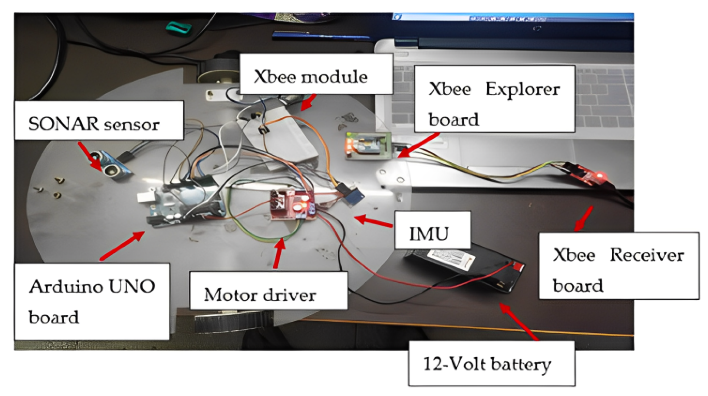
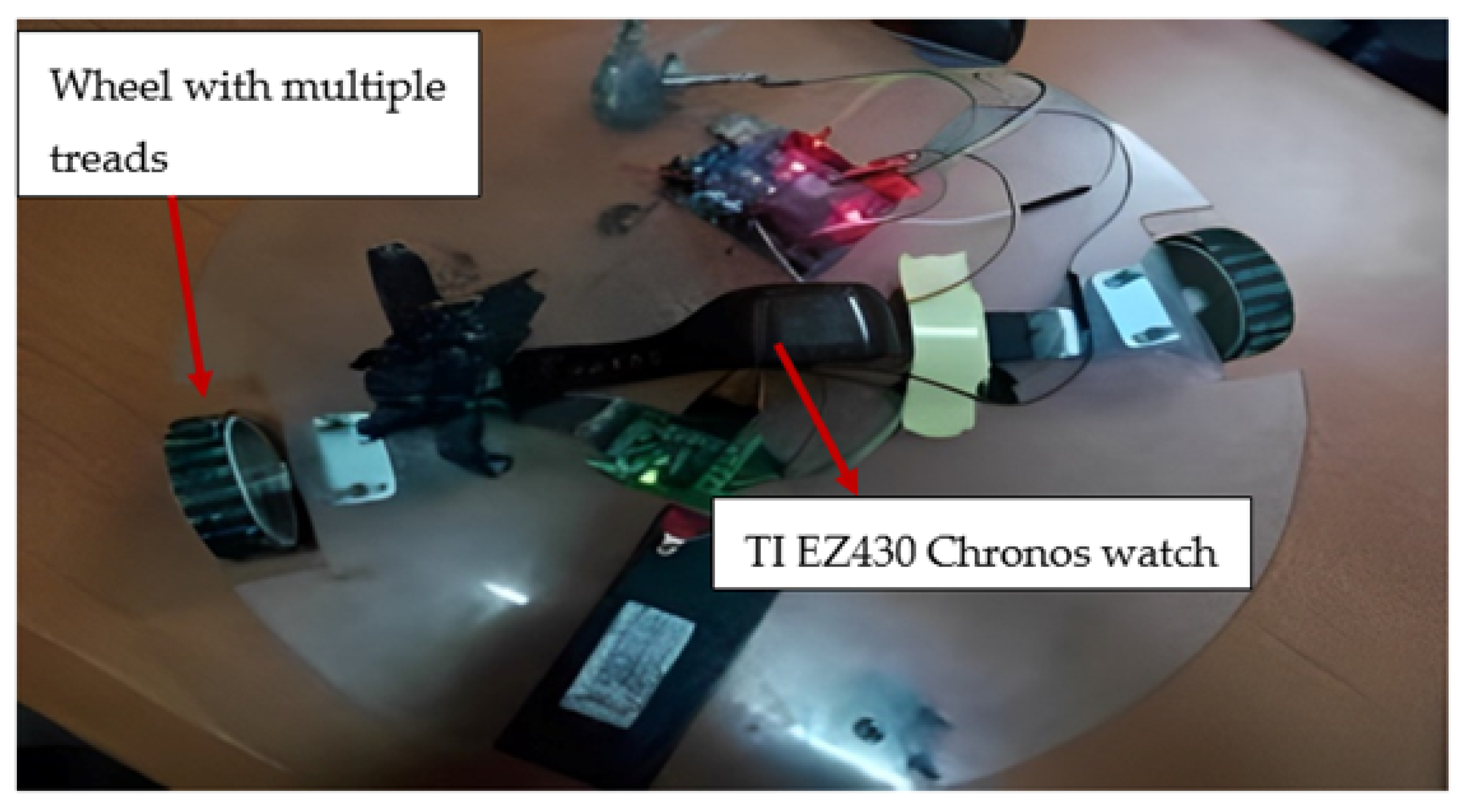
3.1. Robot Design
3.2. Experiments
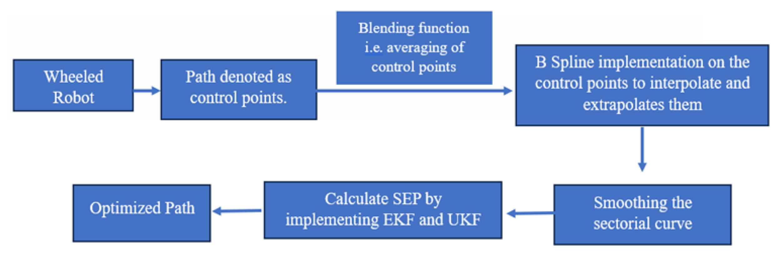
3.3. Mathematical Modelling
- Analyzing discrete time steps and measurements: The time rates (x(t + 1)) of EKF are given in Equation (1). Here, we extend the KF to non-linear system modeling for estimating the state of the system from time ‘t’ to updated time ‘t + 1’. In this equation, F(t)x(t) is the state dynamics function, and G(t)u(t) is the discrete input gain. Its value is preset to 0 based on the discussion given in reference [33].
- Predicting the relation between two states of motion: The next state of a robot is also dependent on its current state, as shown in Equation (2). In this equation, is the initial state, and is the next state of the motion of a robot.
- Predicting the impact of physical parameters: The path of a robot is also dependent on physical parameters such as the robot’s pose, infrared, SONAR, and friction variables. The relationship is shown in Equation (3). In this equation, x, y represents the robot’s pose; , , and represent the Infrared, Sonar, and friction variables in navigation, respectively; and is the projection of the robot’s angular velocity bias gyroscope measurement. The state of motion of a robot on different surfaces is estimated using the outcomes of Equations (1)–(3).
- Impact of Friction: The state of motion of a robot on different surfaces is estimated using the outcomes of Equations (1)–(3). The state and movement of a robot is also dependent on the friction , as calculated in Equation (4). In this equation, and are the surface variables on the X-axis and Y-axis, respectively. and are velocity variables along the X-axis and Y-axis, respectively. T signifies the transpose of the surface and velocity variables.
- Predicting the state of robot without using information about the current state: In some cases, the information about the current state of the robot is unknown. Then, we follow Equations (5) and (5a) to predict its next state. We first estimate the state using the state–space time updation as shown in Equation (5). Then, we obtain the state covariance matrix at time t using the previous covariance matrix at time t. The state covariance matrix holds the uncertainty of the states and contains the covariance of each feature, as shown in Equation (5a) [34]. The state covariance matrix deals with the time stamps and velocities of the robot at time t.
- Measurement Prediction and Minimizing Uncertainty: For precisely estimating the current state of the designed robot, we smoothen the sensor measurements. In the beginning, our state model predicts the next state. Then the measurement prediction model takes the predicted input ( and ) with the sine and cosine components of the state model, to infer new measurements. While making the predictions, we assume that in each time stamp the robot moves with a constant velocity. So, we employed the sine and cosine components to find the next state at a timestamp in the future. The model is defined in Equations (6) and (6a). In these equations, is the estimation state, and is the state variance matrix at time t. Here, the observation model minimizes the error when erroneous data are produced due to sensor failure. Now, the obstacle distance is observed through the measurement matrix defined through measurement vector z and measurement matrix h as given in Equation (7). The state and measurement predictions are associated with each other to resolve the origin uncertainty.
- Navigating the robot: We used estimated innovation covariance and updated measurement for navigating the designed robot. Equation (8) shows the Kalman gain, Equation (9) defines the state update, and Equation (10) provides the updates in state covariance. At the correction state, and are obtained from the prediction state. Here, is calculated by using the state transition state where is user-defined. Next, the Kalman gain or is calculated to represent the trustable value of the state model and measurement variable. Here, matrices are used to handle multiple degrees of freedom that allow the representation of linear relationships between different state variables such as position, velocity, and friction.The value of h approaching 0 indicates that the measurement variable is more trustable than the state model. However, the value of approaching 0 indicates that the state model is more trustworthy than the measurement variable. Next, the estimated data are updated based on values of . Finally, the error covariance is updated for the next iteration. All the parameters are updated in each iteration. Thus, the accuracy of predicted and estimated data improves continuously using the data received from the prediction states [34].
- Predicting sigma Points: UKF uses UT for computing sigma points for two dimensions. It performs transformation by a non-linear density function . This function is defined in Equation (11) [34]. In this research, we use the x and y axis for moving a robot, and consider five sigma points for each dimension. Thus, a matrix () of 2 × 5 is obtained. These sigma points as calculated by UKF are defined in recursive Equations (11a) and (11b). Here, is sigma points matrix, is mean, n is dimensionality, is the scaling factor and ∑ is covariance matrix. The value of n is set at 2 for this research, = 2n + 1, = 3 − n.In Equations (11)–(11b), are the sigma points. Here, , , and are the Infrared, Sonar, and Friction variables in the navigation of the robot respectively, is the projection of the robot’s angular velocity bias. Gyroscope measurement ( and ) are velocity variables along the X-axis and Y-axis, respectively. These are the same as given in Equations (3) and (4). When the sigma points are propagated through non-linear density function , then we first estimate the predicted mean using the state–space time updation as shown in Equation (12). Next, we obtain the predicted covariance matrix, as shown in Equation (13). In this equation, is the predicted covariance, and g is a non-linear function. The state covariance matrix holds the uncertainty of the states and contains the covariance of each feature.
- Updating the state of a robot: In this step, the data captured from the sensors are used to compute the Euclidean distance between the predicted and actual values of mean and covariance [34]. This is defined in Equations (14)–(14b).Here, z denotes the sigma points after transformation in measurement space, is sigma points’ matrix, is mean in measurement space, s is covariance in measurement space, and h is a function that for mapping sigma points to measurement space.
- Predicting error: The error may arise in the prediction step as calculated in Equation (15). In this equation, T is cross-correlation matrix between state space and predicted space, s is the predicted covariance matrix, and K is Kalman Gain. Equation (15a) is like Equation (8) of EKF. Next, the final state is predicted using Equations (16) and (16a). These equations are similar to the Equations (8)–(10) defined in EKF [34]. Here, is mean, ∑ is covariance matrix, is predicted mean, is predicted covariance, K is Kalman gain, z is actual measurement mean, is mean in measurement space, and T is cross correlation matrix.For EKF, the Equations (2) and (3) together are named as state vector equations. These equations are important to predict the impact of modelling parameters. For example, a measurement error may be encountered due to an environmental effect on sensors. Next, Equation (4) is the surface parameter equation. It is used to estimate the motion state of a robot on varying surfaces using outcomes of state vector equations (x, ). Equations (5) and (5a) together are called the initial or starting state equations, respectively. These states are the predecessors of the Kalman filter. Equations 6 and 6a form optimizing state equations. These are used to measure the prediction of the model, which takes the predicted input ( and ) with sine and cosine components of the state model, to infer new measurements. Finally, we fuse Equations (8)–(10) to evaluate as defined in Equation (17). Here, matrices are used to handle multiple degrees of freedom, allowing the representation of linear relationships between different state variables such as position, velocity, and friction.
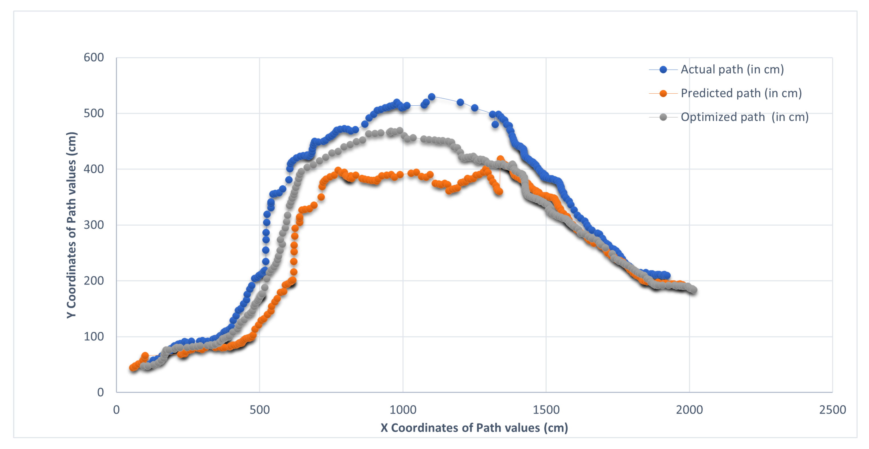
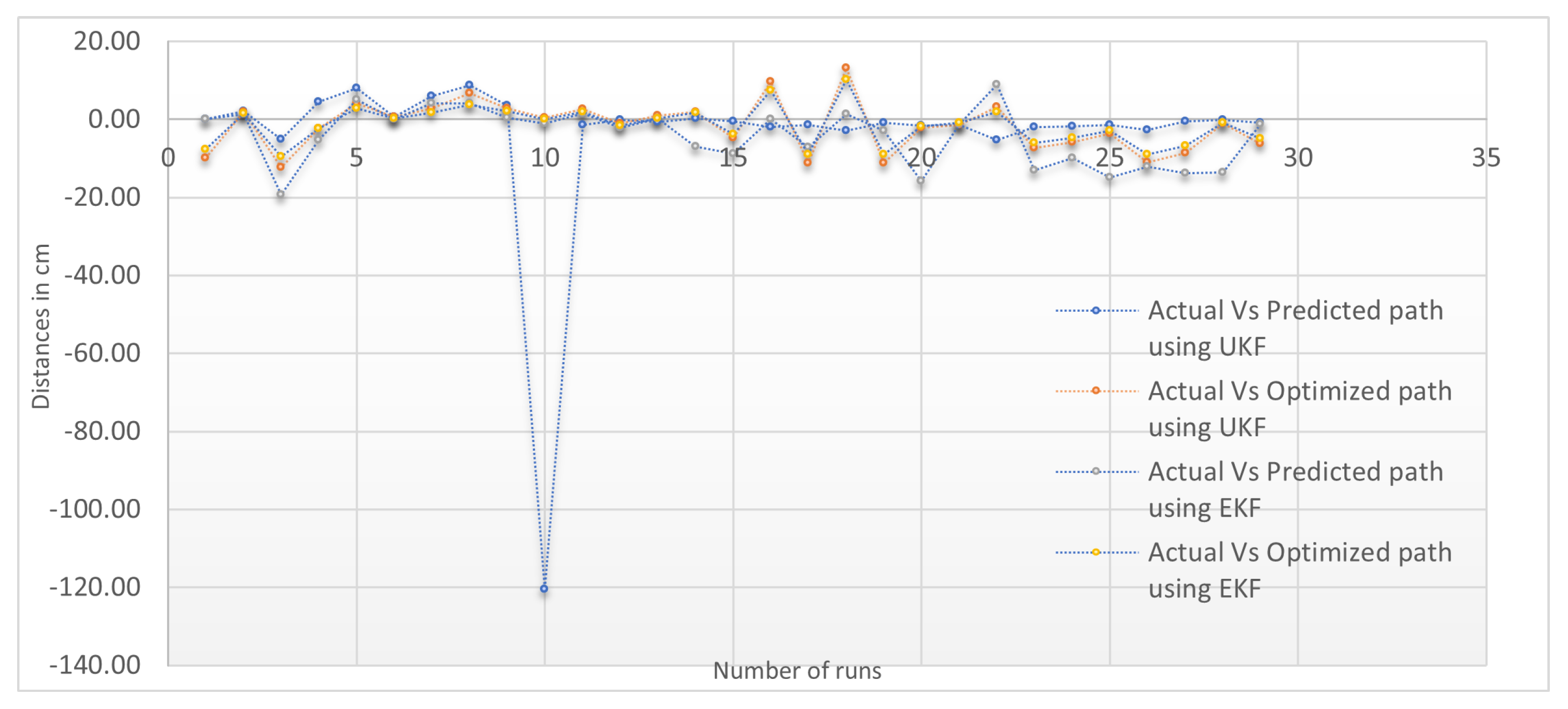
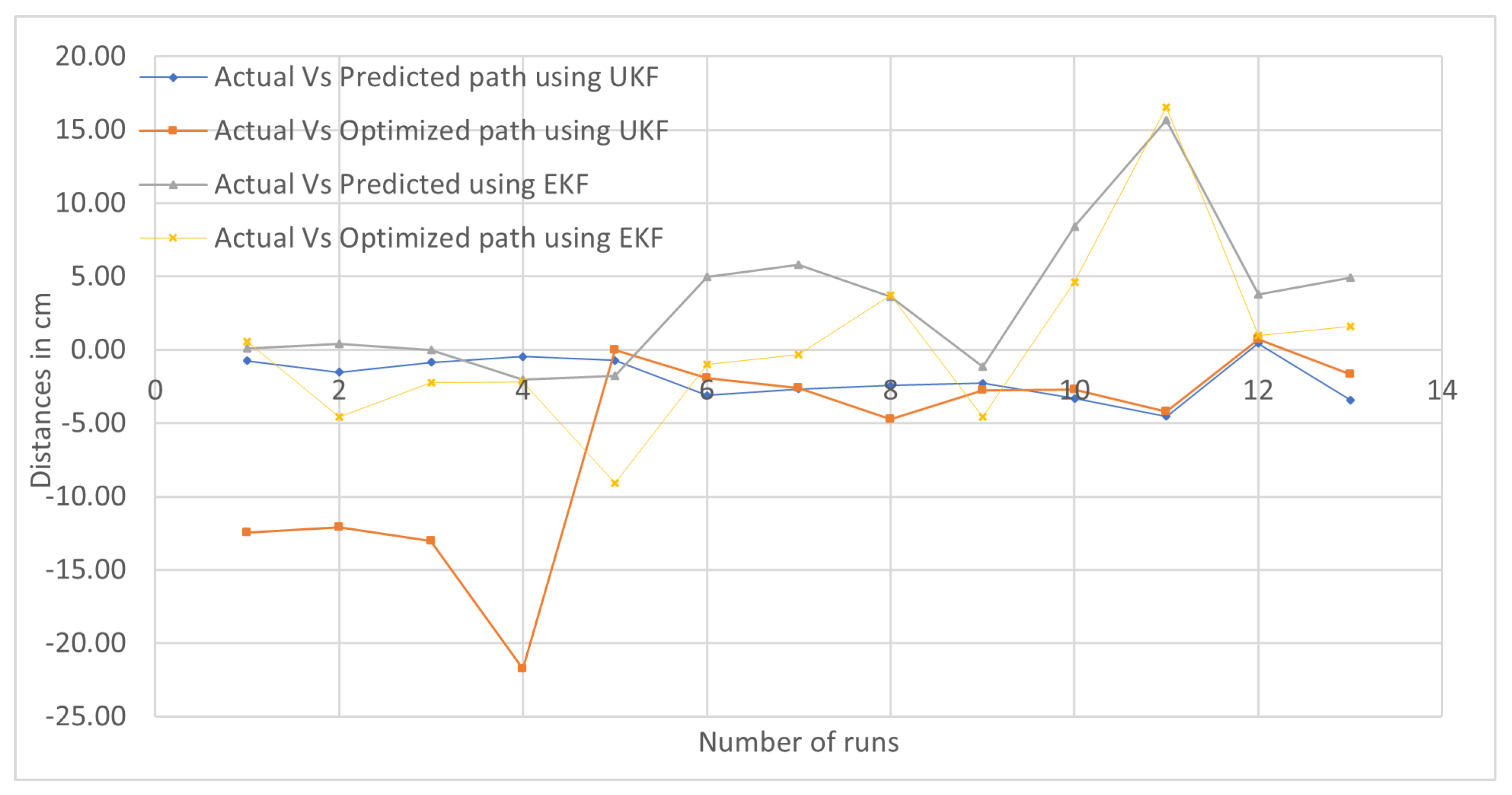
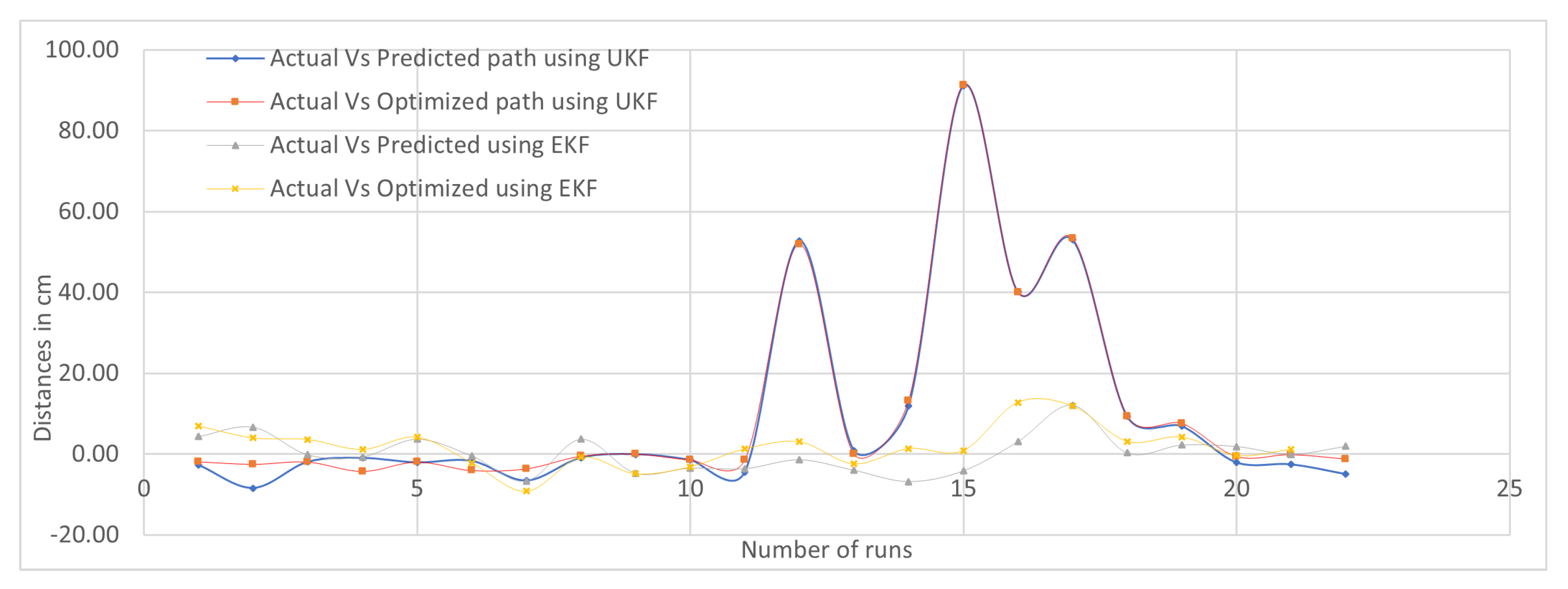
4. Results
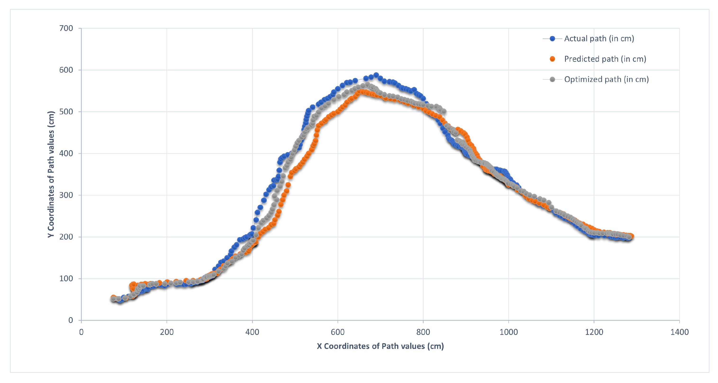
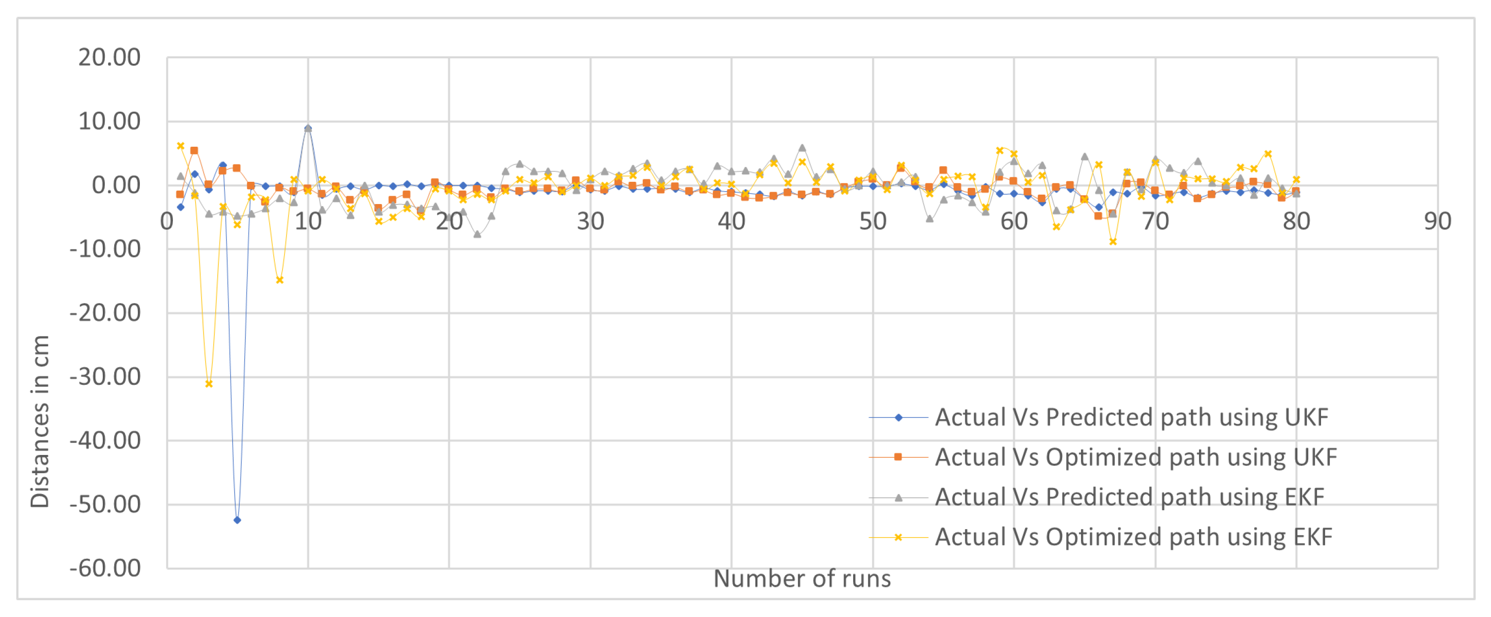
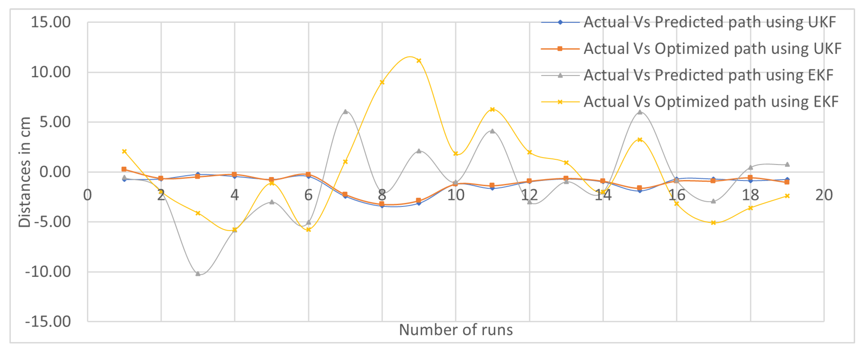
Sectorial-Based Analysis of Predicted, Optimized, and Actual Paths
5. Discussion
6. Conclusions
Supplementary Materials
Author Contributions
Funding
Data Availability Statement
Acknowledgments
Conflicts of Interest
References
- Matharu, P.S.; Ghadge, A.A.; Almubarak, Y.; Tadesse, Y. Jelly-Z: Twisted and coiled polymer muscle actuated jellyfish robot for environmental monitoring. Acta IMEKO 2022, 11, 1–7. [Google Scholar] [CrossRef]
- De Fazio, R.; Katamba, D.M.; Ekuakille, A.L.; Ferreira, M.J.; Kidiamboko, S.; Giannoccaro, N.I.; Velazquez, R.; Visconti, P. Sensors-based mobile robot for harsh environments: Functionalities, energy consumption analysis and characterization. Acta IMEKO 2021, 10, 29. [Google Scholar] [CrossRef]
- Goll, S.; Borisov, A. Interactive model of magnetic field reconstruction stand for mobile robot navigation algorithms debugging which use magnetometer data. Acta IMEKO 2019, 8, 47–53. [Google Scholar] [CrossRef]
- Goll, S.; Zakharova, E. An active beacon-based leader vehicle tracking system. Acta IMEKO 2019, 8, 33–40. [Google Scholar] [CrossRef]
- Li, G.; Qin, D.; Ju, H. Localization of wheeled mobile robot based on extended Kalman filtering. In Proceedings of the MATEC Web of Conferences, Singapore, 15–16 September 2015; p. 01061. [Google Scholar]
- Mittal, R.; Pathak, V.; Mishra, N.; Mithal, A. Localization and Impulse Analysis of Experimental Bot Using eZ430-Chronos. In MARC 2018, Proceedings of the Applications of Computing, Automation and Wireless Systems in Electrical Engineering, Delhi, India, 19–20 July 2018; Springer: Berlin/Heidelberg, Germany, 2019; pp. 711–722. [Google Scholar]
- Mittal, R.; Mishra, N.; Pathak, V. Exploration of Designed Robot in Non Linear Movement Using EKF SLAM and Its Stability on Loose Concrete Surface. Int. J. Eng. Adv. Technol. 2019, 9, 875–878. [Google Scholar] [CrossRef]
- Apriaskar, E.; Nugraha, Y.P.; Trilaksono, B.R. Simulation of simultaneous localization and mapping using hexacopter and RGBD camera. In Proceedings of the 2017 2nd International Conference on Automation, Cognitive Science, Optics, Micro Electro-Mechanical System, and Information Technology (ICACOMIT), Jakarta, Indonesia, 23–24 October 2017; pp. 48–53. [Google Scholar]
- Valade, A.; Acco, P.; Grabolosa, P.; Fourniols, J.Y. A study about Kalman filters applied to embedded sensors. Sensors 2017, 17, 2810. [Google Scholar] [CrossRef]
- Wan, E.A.; Van Der Merwe, R. The unscented Kalman filter for nonlinear estimation. In Proceedings of the IEEE 2000 Adaptive Systems for Signal Processing, Communications, and Control Symposium (Cat. No. 00EX373), Lake Louise, AB, Canada, 4 October 2000; pp. 153–158. [Google Scholar]
- Tang, M.; Chen, Z.; Yin, F. SLAM with Improved Schmidt Orthogonal Unscented Kalman Filter. Int. J. Control Autom. Syst. 2022, 20, 1327–1335. [Google Scholar] [CrossRef]
- Chen, S.; Zhou, W.; Yang, A.-S.; Chen, H.; Li, B.; Wen, C.-Y. An end-to-end UAV simulation platform for visual SLAM and navigation. Aerospace 2022, 9, 48. [Google Scholar] [CrossRef]
- Mittal, R.; Pathak, V.; Gandhi, G.C.; Mithal, A.; Lakhwani, K. Application of machine learning in SLAM algorithms. Mach. Learn. Sustain. Dev. 2021, 9, 147. [Google Scholar]
- Nüchter, A.; Lingemann, K.; Hertzberg, J.; Surmann, H. 6D SLAM—3D mapping outdoor environments. J. Field Robot. 2007, 24, 699–722. [Google Scholar] [CrossRef]
- Mittal, R.; Pathak, V.; Gandhi, G.C.; Mishra, N. Effect of Curve Algorithms on Standard SLAM algorithm for Prediction of Path. Test Eng. Manag. 2020, 83, 1196–1201. [Google Scholar]
- Liu, M.; Huang, S.; Dissanayake, G. Feature based SLAM using laser sensor data with maximized information usage. In Proceedings of the 2011 IEEE International Conference on Robotics and Automation, Shanghai, China, 9–13 May 2011; pp. 1811–1816. [Google Scholar]
- Kysar, S.; Young, P.; Kurup, A.; Bos, J. C-SLAM: Six degrees of freedom point cloud mapping for any environment. In Proceeding of the Autonomous Systems: Sensors, Processing, and Security for Vehicles and Infrastructure, Online, 27 April–9 May 2020; pp. 98–112. [Google Scholar] [CrossRef]
- Dhiman, N.K.; Deodhare, D.; Khemani, D. Where am I? Creating spatial awareness in unmanned ground robots using SLAM: A survey. Sadhana 2015, 40, 1385–1433. [Google Scholar] [CrossRef]
- Dryanovski, I.; Morris, W.; Kaushik, R.; Xiao, J. Real-time pose estimation with RGB-D camera. In Proceedings of the 2012 IEEE International Conference on Multisensor Fusion and Integration for Intelligent Systems (MFI), Hamburg, Germany, 13–15 September 2012; pp. 13–20. [Google Scholar]
- Meier, K.; Chung, S.J.; Hutchinson, S. Visual-inertial curve simultaneous localization and mapping: Creating a sparse structured world without feature points. J. Field Robot. 2018, 35, 516–544. [Google Scholar] [CrossRef]
- Molina Martel, F.; Sidorenko, J.; Bodensteiner, C.; Arens, M.; Hugentobler, U. Unique 4-DOF relative pose estimation with six distances for UWB/V-SLAM-based devices. Sensors 2019, 19, 4366. [Google Scholar] [CrossRef]
- You, W.; Li, F.; Liao, L.; Huang, M. Data fusion of UWB and IMU based on unscented Kalman filter for indoor localization of quadrotor UAV. IEEE Access 2020, 8, 64971–64981. [Google Scholar] [CrossRef]
- Zhang, P.; Li, R.; Shi, Y.; He, L. Indoor navigation for quadrotor using rgb-d camera. In Proceedings of the 2018 Chinese Intelligent Systems Conference, Wenzhou, China, 11 January 2019; Springer: Singapore, 2019; Volume 2, pp. 497–506. [Google Scholar]
- Mittal, R.; Pathak, V.; Goyal, S.; Mithal, A. GP-GPU. In Recent Trends in Communication and Intelligent Systems: Proceedings of ICRTCIS 2019, Jaipur, India, 22–23 October 2021; Springer: Berlin/Heidelberg, Germany, 2020; p. 157. [Google Scholar]
- Fink, A.; Lange, J.; Beikirch, H. Radio-based indoor localization using the eZ430-Chronos platform. In Proceedings of the 2012 IEEE 1st International Symposium on Wireless Systems (IDAACS-SWS), Offenburg, Germany, 20–21 September 2012; pp. 19–22. [Google Scholar]
- Fuentes-Pacheco, J.; Ruiz-Ascencio, J.; Rendón-Mancha, J.M. Visual simultaneous localization and mapping: A survey. Artif. Intell. Rev. 2015, 43, 55–81. [Google Scholar] [CrossRef]
- Sakenas, V.; Kosuchinas, O.; Pfingsthorn, M.; Birk, A. Extraction of semantic floor plans from 3D point cloud maps. In Proceedings of the 2007 IEEE International Workshop on Safety, Security and Rescue Robotics, Rome, Italy, 27–29 September 2007; pp. 1–6. [Google Scholar]
- Martinez, A.M.; Kak, A.C. Pca versus lda. IEEE Trans. Pattern Anal. Mach. Intell. 2001, 23, 228–233. [Google Scholar] [CrossRef]
- Viola, P.; Jones, M. Rapid object detection using a boosted cascade of simple features. In Proceeding of the 2001 IEEE Computer Society Conference on Computer Vision and Pattern Recognition, Kauai, HI, USA, 8–14 December 2001. [Google Scholar]
- Bonato, V.; Marques, E.; Constantinides, G.A. A floating-point extended kalman filter implementation for autonomous mobile robots. J. Signal Process. Syst. 2009, 56, 41–50. [Google Scholar] [CrossRef]
- Mittal, R.; Mishra, N.; Pathak, V. A review of robotics through cloud computing. J. Adv. Robot. 2018, 5, 1–11. [Google Scholar]
- Briand, T.; Davy, A. Optimization of image B-spline interpolation for GPU architectures. Image Process. Line 2019, 9, 183–204. [Google Scholar] [CrossRef]
- Dorj, B.; Hossain, S.; Lee, D.J. Highly curved lane detection algorithms based on Kalman filter. Appl. Sci. 2020, 10, 2372. [Google Scholar] [CrossRef]
- Yang, C.; Shi, W.; Chen, W. Comparison of unscented and extended Kalman filters with application in vehicle navigation. J. Navig. 2017, 70, 411–431. [Google Scholar] [CrossRef]
- Tian, C.; Liu, H.; Liu, Z.; Li, H.; Wang, Y. Research on Multi-Sensor Fusion SLAM Algorithm Based on Improved Gmapping. IEEE Access 2023, 11, 13690–13703. [Google Scholar] [CrossRef]
- Bai, J.; Du, J.; Li, T.; Chen, Y. Trajectory tracking control for wheeled mobile robots with kinematic parameter uncertainty. Int. J. Control Autom. Syst. 2022, 20, 1632–1639. [Google Scholar] [CrossRef]
- Naab, C.; Zheng, Z. Application of the unscented Kalman filter in position estimation a case study on a robot for precise positioning. Robot. Auton. Syst. 2022, 147, 103904. [Google Scholar] [CrossRef]


| No. of Pulse | Actual Pose | Predicted Pose | Optimized Pose | Actual | Predicted | Optimized | |||
|---|---|---|---|---|---|---|---|---|---|
| X-Axis | Y-Axis | X-Axis | Y-Axis | X-Axis | Y-Axis | Path | Path | Path | |
| 1 | 95 | 51 | 79 | 53 | 87 | 52 | 3.6055 | 2.2360 | 2 |
| 2 | 99 | 55 | 104 | 54 | 102 | 54 | 5.6568 | 25.0199 | 15.1327 |
| 3 | 110 | 57 | 120 | 58 | 115 | 58 | 11.1803 | 16.4924 | 13.6014 |
| Component Used [35] | Approximately Cost | Components Used in Our Design | Exact Cost |
|---|---|---|---|
| 2D Lidar Sensor | INR 10,000/- | Ez 430 Chronos Watch | INR 5000/- |
| RGB-D Camera | INR 8000/- | IMU, SONAR, IR | INR 1300/- |
| Nvidia Jetson Nano Board | INR 15,000/- | Arduino Board with overhead | INR 3000/- |
| WiFi Module | INR 400/- | Xigbee kit with Xbee base and 1 device module | INR 3200/- |
| Encoder Gearmotor | INR 2000/- | DC Motor with module | INR 510/- |
| McNam Wheel | INR 6000/- (100 mm) | Castor wheel with 2 rubber wheels | INR 600/- |
| Total Cost (Approximately) | INR 41,400 | Total cost | INR 13,610/- |
| Observation Points | Actual Distance | Predicted Distance | Optimized Distance | Actual-Predicted | Actual-Optimized | Actual-Predict/ Actual (%) | Actual-Optimized/ Actual (%) |
|---|---|---|---|---|---|---|---|
| 1 | 482.8 | 731 | 580 | −249 | −97 | −51.4872 | −20.1326 |
| 2 | 600 | 643 | 666 | −42 | −66 | −7.05814 | −11.0245 |
| 3 | 179 | 205 | 258 | −26 | −79 | −14.2586 | −44.2212 |
| 4 | 480 | 256 | 239 | 224 | 241 | 46.68958 | 50.20833 |
| 5 | 532 | 644 | 586 | −112 | −54 | −21.0526 | −10.1504 |
| 6 | 130 | 153 | 150 | −23 | −20 | −9.44104 | −3.14521 |
| Sum | 2404.29 | 2631.28 | 2479.91 | −9.43467 | −6.41092 |
| Observation Points | Actual Distance | Predicted Distance | Optimized Distance | Actual-Predicted | Actual-Optimized | Actual-Predict/ Actual (%) | Actual-Optimized/ Actual (%) |
|---|---|---|---|---|---|---|---|
| 1 | 380 | 623 | 470 | −243 | −90 | −64.0361 | −23.658 |
| 2 | 562 | 504 | 512 | 59 | 50 | 10.41694 | 8.929528 |
| 3 | 149 | 106 | 145 | 43 | 4 | 28.67205 | 2.670958 |
| 4 | 205 | 201 | 168 | 3 | 37 | 1.696848 | 18.09336 |
| 5 | 434 | 457 | 484 | −23 | −50 | −5.26495 | −11.4537 |
| 6 | 101 | 121 | 99 | −20 | 3 | −19.3412 | 2.653122 |
| Sum | 1935 | 1936 | 1827 | −797606 | −0.46079 |
| S.No. | Deviation in Paths | Key I (cm) | Key II (cm) | Key III (cm) | Key IV (cm) | Key V (cm) | Key VI (cm) | Average SEP Observation Points |
|---|---|---|---|---|---|---|---|---|
| 1. | EKF (Actual vs. Predicted) | −4.19 | 0.83 | 3.28 | 0.16 | −0.12 | 1.33 | 1.65 |
| 2. | EKF (Actual vs. Optimized) | −1.55 | 0.71 | 0.31 | 1.69 | −0.62 | 1.88 | 1.13 |
| 3. | UKF (Actual vs. Predicted) | −4.12 | −0.60 | −1.97 | 10.22 | −1.28 | 0.48 | 3.11 |
| 4. | UKF (Actual vs. Optimized) | −1.68 | −0.93 | −6.10 | 10.98 | −0.68 | 0.75 | 3.52 |
| Parameters | 4-DoF and 6-DoF | 8-DoF |
|---|---|---|
| Diverse Surfaces | The wheel profile of the Turtlebot has independent spring suspension. Thus, the height of two wheels varies when it is moved on pebbled surface. This may lead to misbalancing and falling of Turtlebot. | The wheel profile of the designed robot makes it effective to move on pebbled surface [7] |
| Grip on surface | The presence of a single cut in the center leads to reduced grip () on the surface, making it challenging to control the speed of both wheels while moving on that surface. = F_friction/F_normal Here, F_friction represents the friction between a wheel and a surface, while F_normal denotes the force that acts perpendicular to the surface on which the wheel is positioned. | The wheels have more than four nearby thin cuts that improve grip on various surfaces. The wheel profile is designed without suspension, making it rigid and fixed on a round plate. Additionally, each wheel generates different power, enabling the robot to maneuver effectively on diverse surfaces. The wheels individually can generate power. So, we can control their speeds independently. |
| Remote navigation | Turtlebot does not have built in remote area network (RAN). Its’ external integration may lead to battery and power loss issues. | Our wheeled robot supports APIs-based communication with the hardware using built in RAN. |
| Parameters | Curve SLAM | Open Key Frame-Based Visual Inertial SLAM (OKVIS) | Stereo Version of the Parallel Tracking and Mapping (SPTAM) | Proposed Method |
|---|---|---|---|---|
| Control points | 220 | 345,340 | 138,403 | 240 |
| SEP | 2.57 m | 4.68 m | 2.58 m | 1.652 cm Actual and predicted position of robot |
| 1.125 cm Actual and optimized position of robot |
Disclaimer/Publisher’s Note: The statements, opinions and data contained in all publications are solely those of the individual author(s) and contributor(s) and not of MDPI and/or the editor(s). MDPI and/or the editor(s) disclaim responsibility for any injury to people or property resulting from any ideas, methods, instructions or products referred to in the content. |
© 2023 by the authors. Licensee MDPI, Basel, Switzerland. This article is an open access article distributed under the terms and conditions of the Creative Commons Attribution (CC BY) license (https://creativecommons.org/licenses/by/4.0/).
Share and Cite
Mittal, R.; Rani, G.; Pathak, V.; Chhikara, S.; Dhaka, V.S.; Vocaturo, E.; Zumpano, E. Low-Cost Multisensory Robot for Optimized Path Planning in Diverse Environments. Computers 2023, 12, 250. https://doi.org/10.3390/computers12120250
Mittal R, Rani G, Pathak V, Chhikara S, Dhaka VS, Vocaturo E, Zumpano E. Low-Cost Multisensory Robot for Optimized Path Planning in Diverse Environments. Computers. 2023; 12(12):250. https://doi.org/10.3390/computers12120250
Chicago/Turabian StyleMittal, Rohit, Geeta Rani, Vibhakar Pathak, Sonam Chhikara, Vijaypal Singh Dhaka, Eugenio Vocaturo, and Ester Zumpano. 2023. "Low-Cost Multisensory Robot for Optimized Path Planning in Diverse Environments" Computers 12, no. 12: 250. https://doi.org/10.3390/computers12120250
APA StyleMittal, R., Rani, G., Pathak, V., Chhikara, S., Dhaka, V. S., Vocaturo, E., & Zumpano, E. (2023). Low-Cost Multisensory Robot for Optimized Path Planning in Diverse Environments. Computers, 12(12), 250. https://doi.org/10.3390/computers12120250