


The Doubly Linked Tree of Singly Linked Rings: Providing Hard Real-Time Database Operations on an FPGA


Abstract
:1. Introduction
1.1. Motivation
1.1.1. Hard Real-Time Databases
1.1.2. Operations on Tables
1.2. Issues to Address
1.2.1. DB-Operations vs. Hard Real-Time
1.2.2. Dynamic Data Width
1.2.3. Memory Allocation and Deallocation
1.2.4. Performance on FPGAs
1.3. Contribution
1.4. Content
2. Related Work
2.1. Real-Time Databases
2.2. FPGAs and Databases
2.3. Hard Real-Time and Hardware Data Structures
2.4. Dynamic Memory Management in FPGAs
3. System Model
3.1. Notation
- Control Nodes N are used to manage the data structure.
- Data Nodes N contain user data in their data field.
 , is the name of the node viewed as data node, while is the same node’s name viewed as control node. Accessing a node’s content is denoted as : A .next is the next pointer of control node A and B .data is the data field of data node B. Pointers hold the address of a node and can either be contained in the next field ➞ or the data field
  . NULL-pointers are marked with
  .
.3.2. Memory Organization
3.2.1. Memory Hardware
3.2.2. Memory Management
3.2.3. Modifications to the Memory Manager
3.3. Hard Real-Time Databases vs. Unknown Amounts of Data
3.3.1. Database Content
- Insert inserts a new row of data into an existing table.
- In a hard RTDB, a transaction’s execution must not exceed its deadline.
3.3.2. Database Schema
3.4. Limitations
4. The Doubly Linked Tree of Singly Linked Rings
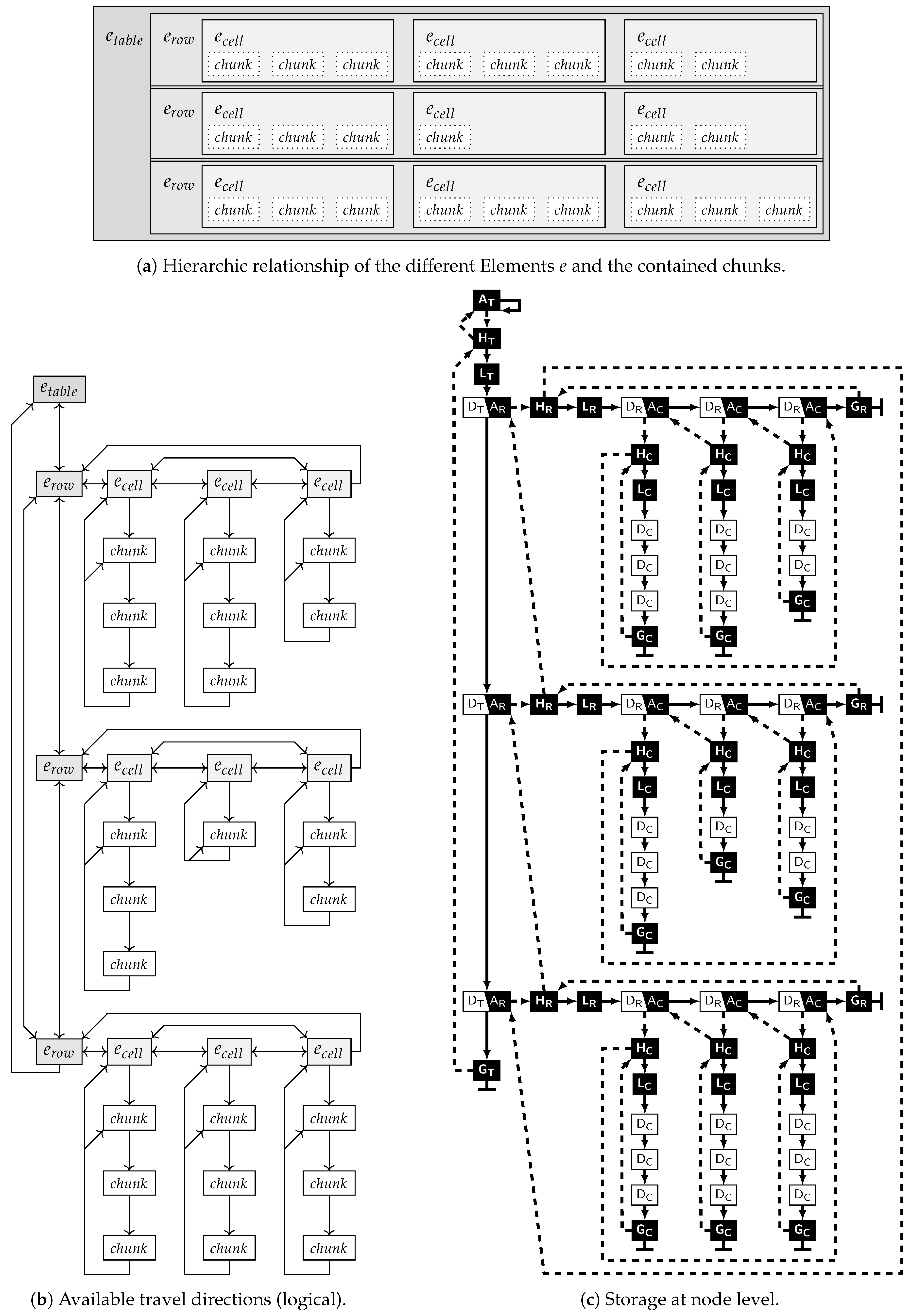
4.1. The “Element”
4.1.1. Requirements
4.1.2. Storage
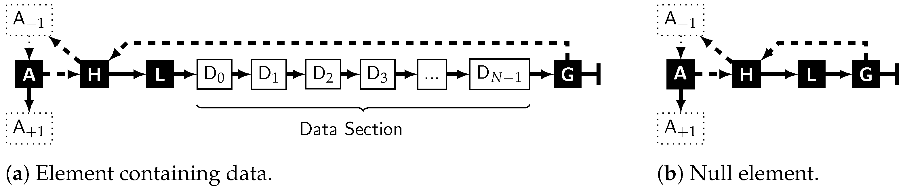
| A | The anchor provides a stable address, while the element’s content might change over time. The address of the element will be used synonymous to the anchor’s address. |
| H | The hierarchical node allows hierarchy ascent and reverse reading. Its data pointer creates a link to the previous anchor and is also called hierarchical pointer of the element. |
| L | The cyclic length node, containing the number of nodes in the cyclic part of the element, which can be derived either as (the data nodes plus the three control nodes in the loop) or (count all nodes, subtract the anchor, which is not part of the loop). It allows usage of the hard real-time memory management from [50], which is also where counting only the cyclic part originates from. |
| D | As many data nodes N as required for storage of the element’s content in their datafield. This part shall be omitted for an explicitly empty element where N = 0 (Figure 3b). |
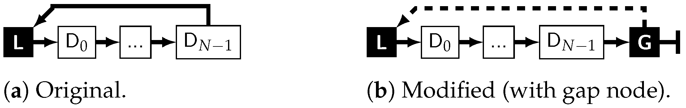
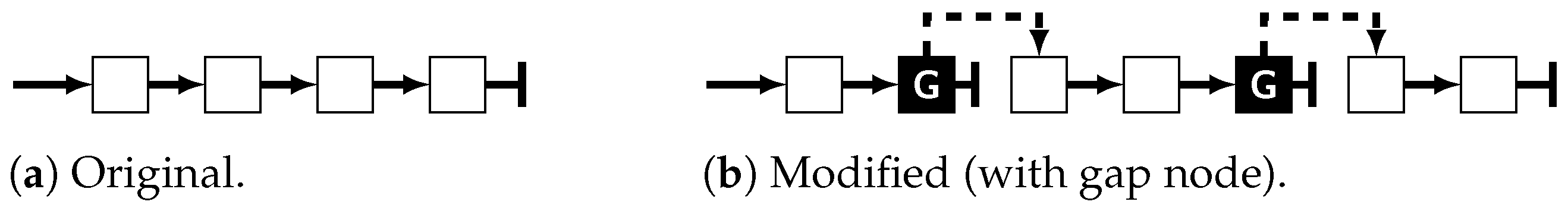
| G | The gap node, marking the end of the data section of the element and closing the loop back to the hierarchical node via its data-pointer. Its next-pointer is always NULL. Therefore, the module reading an element does not have to count nodes and permanently compare this to N − 3 while iterating just to detect the end of the data section. |
4.1.3. Hierarchical Linking
 comes into play: it stores a link to the previous element in ’s data section (wrapping around the ring; itself if it is the only element). This allows reverse reading of the data section of . It also introduces the possibility of hierarchic ascent from a child to its parent via ’s predecessor.
4.2. Practical Example: Building a Table
4.2.1. Hierarchy
4.2.2. Linking Elements
4.3. Base Operations
to  to
to  ’s next-pointer to wrap around from the last child of to the first.
| Algorithm 1: InsertAfter(, , ) |
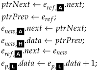 |
4.4. Derived Operations
| Algorithm 2: LastChild() |
 |
| Algorithm 3: InsertAsFirst(, )) |
 |
| Algorithm 4: InsertAsLast |
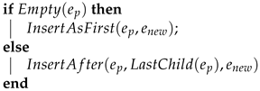 |
| Algorithm 5: InsertBefore(, , ) |
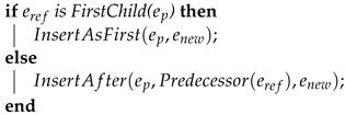 |
| Algorithm 6: FreeElement(e) |
 |
| Algorithm 7: DeleteChild(, )—Without Hierarchy Limit |
 |
| Algorithm 8: DeleteChild(, , )—Hierarchy Limited |
 |
 .
.| Algorithm 9: Update(, ) |
 |
 of the new element is not strictly required for this operation and could be omitted in practical implementation if an accordingly modified version of FreeElement() is provided. It is still included in the algorithm to preserve this paper’s convention of only passing complete elements as parameters.
4.5. Other Properties (Not Necessarily Real-Time)
4.5.1. Arbitrary Entry Cyclic Access
4.5.2. Hierarchic Ascent
5. Real-Time Operation (Proof)
5.1. Prerequisites
5.1.1. Basic Access
5.1.2. Memory Management
5.1.3. Storing a Data Stream in an Element
5.1.4. Primary Key Access & Reading Data from an Element
5.1.5. Accessibility of the Control Nodes
e H ➞ e L . □5.2. Base Operations
5.3. Derived Operations
5.4. Storing a Hierarchy
6. Experimental Results
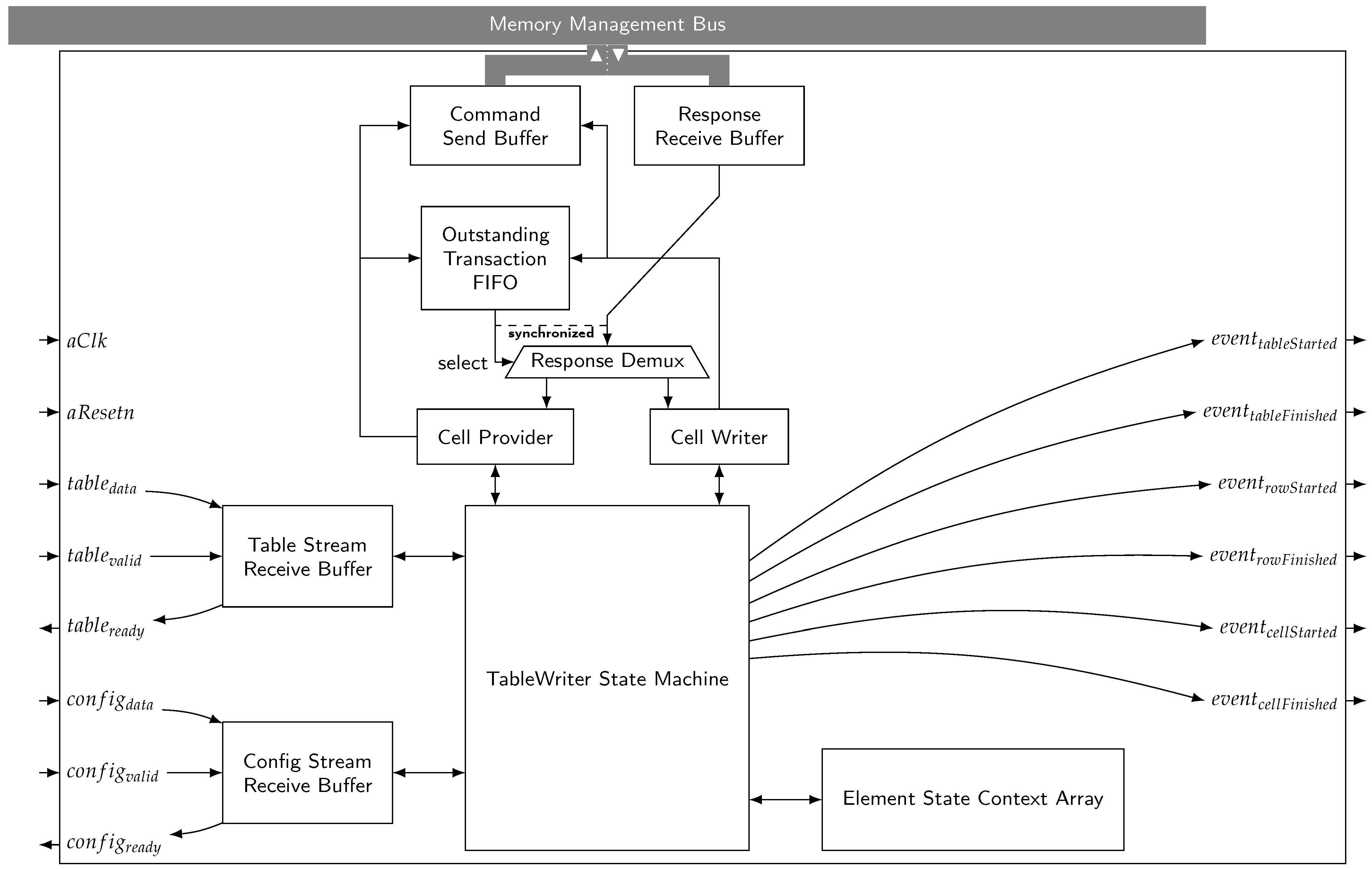
6.1. Example: The TableWriter
- Table Writer State Machine The Table Writer State machine is the central control unit. It reads the received table data—annotated with hierarchy information in the form this transfer is the last of the current cell/row/table—from the Table Stream Receive Buffer, which can store a single chunk of data. Its interaction with the central memory management bus (also providing memory read/write) is controlled via the Cell Provider and Cell Writer units. The state machine itself is implemented as a context switching state machine (as described in Appendix B). The TableWriter uses three contexts—one for each of the hierarchy levels Table, Row, Cell. Every context in represents the current operation on an element at this level. It stores the state of the single level state machine (shown in Figure 6), as well as the addresses of the element’s anchor nodes, the current cyclic node count, the addresses of a few ‘virtual’ nodes (the last node before G , the first data node, the current data node, the previously processed node, and the first child’s H node) and finally a boolean determining if the element has been completed.
- Cell Provider & Cell Writer To simplify interaction with the memory management bus, the TableWriter utilizes two dedicated units to allocate new memory (Cell Provider) and write data to memory (Cell Writer). The Memory Provider simply requests a new memory cell by sending the memory managers PickUpFreeCell command and storing the address of the allocated cell returned by the response. When the Table Writer State Machine requires a new memory cell, it takes the one previously allocated by the Cell Provider, marking the Cell Provider as empty—which triggers the Cell Provider to request a new memory cell. In contrast, the Memory Writer only acts on demand: The Statemachine provides a new write task by passing the target address, the data to write and a strobe signal to the Memory Writer which decides whether the whole memory cell, only the data field or only the next field shall be written (This was not mentioned in Section 3.2.3 since it is not necessary for the doubly linked tree of singly linked rings itself. We still use it in the practical evaluation as our prototype already utilizes this updated version of the memory manager (a paper on the updated manager is in preparation). This does not change the systems ability of hard real-time operation since the strobe signal is simply translated to the AXI byte strobe of a single transfer. It does, however, slightly improve the latency, since a partial write would otherwise require knowledge of the non-written content, which can sometimes only be acquired by performing an additional read before writing the cell.).
- Buffers The send/receive buffers shown in Figure 5 use a slightly relaxed (We ignore the fact that AXI expects the data field to have a multiple of eight bits as its width.) version of the AXI-Stream protocol by ARM [51]. A buffer x accepts new data if it is empty and the data on is marked as valid via . Clearing the buffer automatically signals to the outside that new data can be received via . This means that transfers happen when .
- Outstanding Transaction FIFO & Response Demux Since the memory management bus is used both by the Cell Provider and the Cell Writer, responses have to be directed towards the authors of their corresponding commands. Every time a command is sent to the Command Send Buffer, the command’s author (CELL_WRITER or CELL_PROVIDER) is inserted into the Outstanding Transaction Fifo. When a response arrives on the Response Receive Buffer, the Outstanding Transaction Fifos output is used to decide where to route the response via the Response Demux demultiplexer.
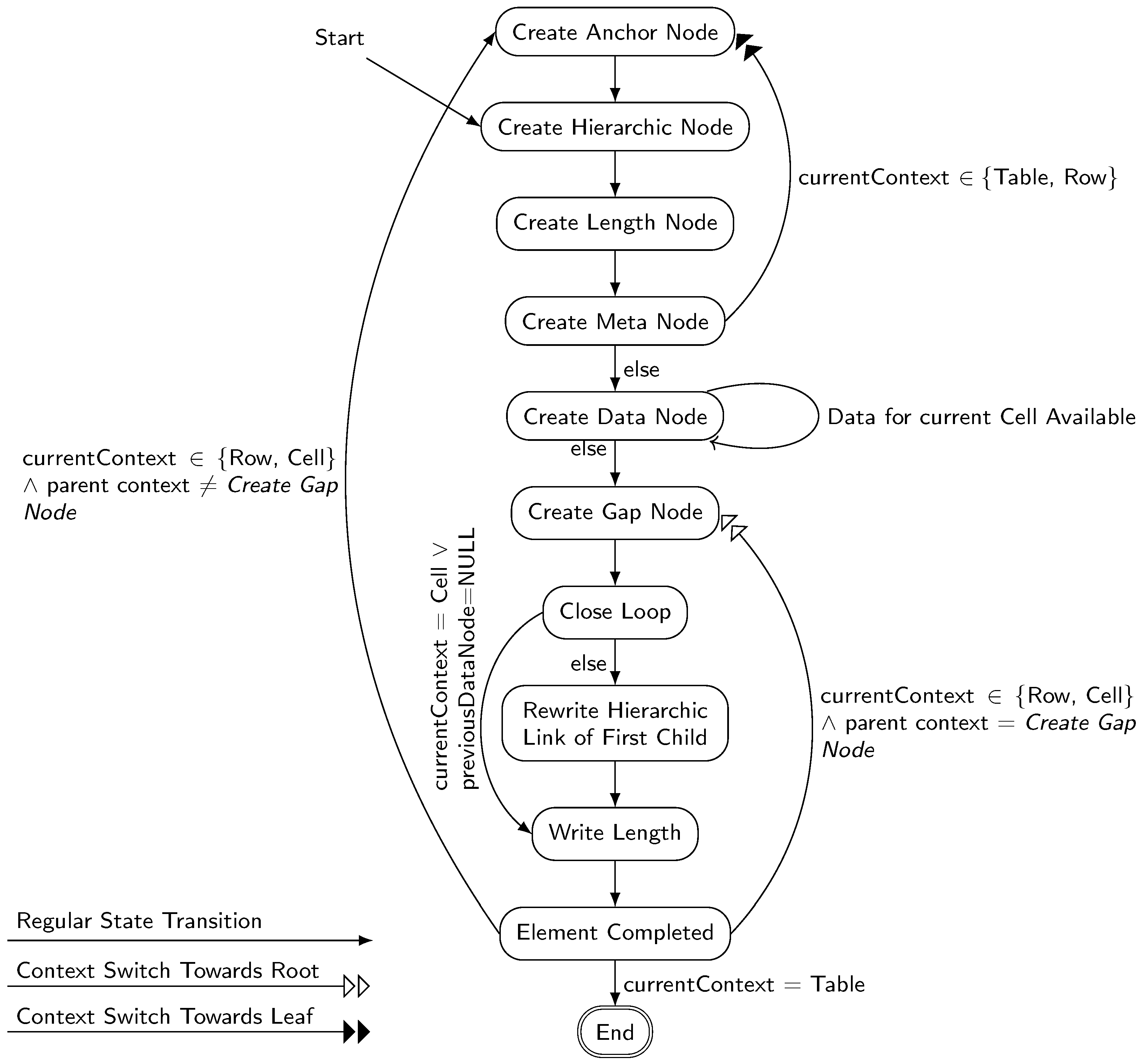
- Start Since the TableWriter receives the anchor node via its Config Stream input, the state machine skips the anchor creation state on the table layer and directly starts with creating and connecting the hierarchic node H to it in Create Hierarchic Node.
- Create Anchor Node Creates A
- Create Hierarchic Node Creates H and links A .next to H .
- Create Length Node & Create Meta Node Next, Create Length Node creates the length node. At Create Meta Node (or Create Length Node if you were to implement our original algorithm), the first decision has to be made: if the current context level is not at the leaf layer (Cell), we will perform a context switch towards the leaf layer (either Table Row or Row Cell). In the new context, the state machine is initialized (resetting the whole context) to start with a fresh element at Create Anchor Node. If instead we are at leaf level, we can start with filling in the streamed data corresponding to the current element by going to Create Data Node.
- Create Data Node This state creates and appends new data nodes as long as new data are received on the Table Stream Receive Buffer. As soon as the received data are marked to be the last chunk in the current hierarchy level (e.g., the last transfer of a Row), the state machine proceeds to Create Gap Node. If the data are also marked with ’end’ markers for higher hierarchy levels (e.g., end of cell + end of row), all affected contexts move to the Create Gap Node state as well.
- Create Gap Node Here, G is created and attached.
- Close Loop This step closes the loop/cyclic part of the element. If the current element has at least one child, we have to update the child’s hierarchic link in Rewrite Hierarchic Link of First Child. Otherwise (either we are a Cell level and/or there was not child element), we can directly proceed with Write Length.
- Rewrite Hierarchic Link of First Child Update the H node of the first child. This is only possible after all following childs have been processed since its data-pointer links to the last child’s A .
- Write Length Updates the L node to the actual cyclic node count.
- Element Completed As soon as an element is completed, the state machine has to decide whether the whole table writing task has been completed (current context is Table) or further processing is required. If the context if one of the lower layers Row or Cell, we have two possibilities:
- The parent context expects further data In this case (parent context ≠ Create Gap Node), the parent context has not received a corresponding ’your hierarchic level ends here’ marker from the Create Data Node stage. Therefore, it can directly proceed at the current level by creating the anchor node for the next child of its parent.
- The parent context is about to be finished Here, the parent context is already at Create Gap Node as the received data marked the current element as the last child of the parent. We therefore continue by switching the context level back up towards the root level (Cell ▹▹ Row or Row Table) and proceeding with the parents gap node creation.
- End The whole table has been fully written.
6.2. Simulation
6.2.1. Test: Moving Larger Cell in a Square Table
- Condition In this test, we write equally sized variations of a 4 × 4 table to memory. In each run, all cells except a single focused cell are of size one, while the focused cell consists of eight memory cells. The testbench performs 16 runs which represent the 16 possible positions of the focused cell.
- Hypothesis Since all tables consist of an equal count of elements with constant total size, we expect to see identical execution times as well as identical memory usage for all runs. The memory usage is expected to bewhich can be derived as follows: We need one element containing the rows, one for each of the four rows containing the cells and one per cell. The size of each element (ignoring the payload) is #{ A , H , L , M , G } Since the payload of the leaf elements is always handled equally independent of which element it is contained in, it is possible to simply sum up the individual payloads of the focused and the non-focused cells. The payload of the non-leaf elements consists exclusively of anchor nodes, which have already been counted in their respective elements.memtable = (1 + 4 + 16) · #{ A , H , L , M , G } + 8 + (16 − 1) = 128 memory cells,
- Result Our simulation showed equal execution times of 1333 clock cycles for all runs. The memory consumption after writing the table was always at 128 memory cells.
6.2.2. Test: Moving Larger Cell in Non-Square Table
- Condition Since the first test had an identical number of rows and columns, it might not show problems if the TableWriter would have a preference for square table structures. The following test will evaluate this by applying the same concept to a 7 × 5 table.
- Hypothesis If the TableWriter works correctly it should again show identical executions times and memory usages. Memory usage should be memory cells.
- Result All test runs show identical execution times of 2698 clock cycles. The memory usage has the expected value of 257 memory cells. The maximum outstanding transaction count was again at eight transactions.
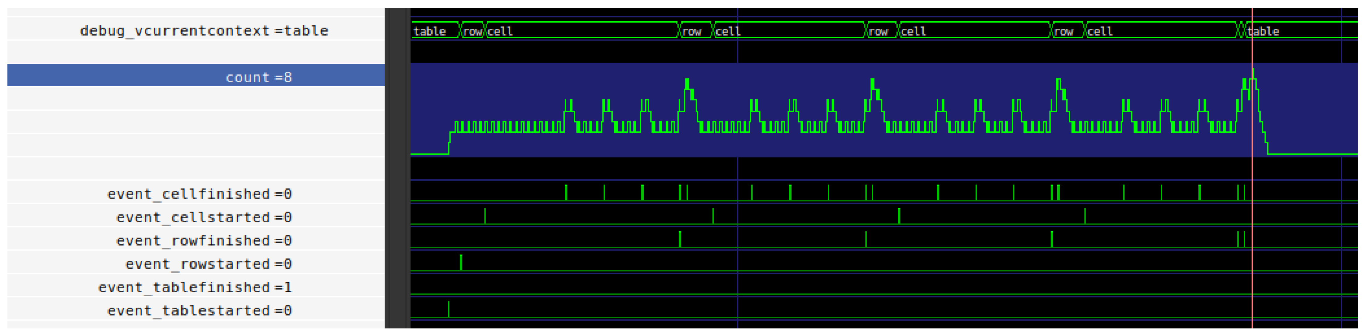
6.2.3. Test: Table with Varying Payload and Table Size
- Condition This time we repeated the first test (4 × 4 table with focused cell), but varied the size of the focused cell. We also completed a second iteration with a 3 × 4 table to test if the table schema has any influence on the execution time required for storing additional payload.
- Hypothesis Since the execution time for creating the table schema (the higher hierarchy levels) is expected to be independent of the execution time for storing the payload in leaf nodes, we expect linearly rising execution times for the payload with a constant offset for the tables schema. The execution time per additional chunk should be the same for the two different table schemas.
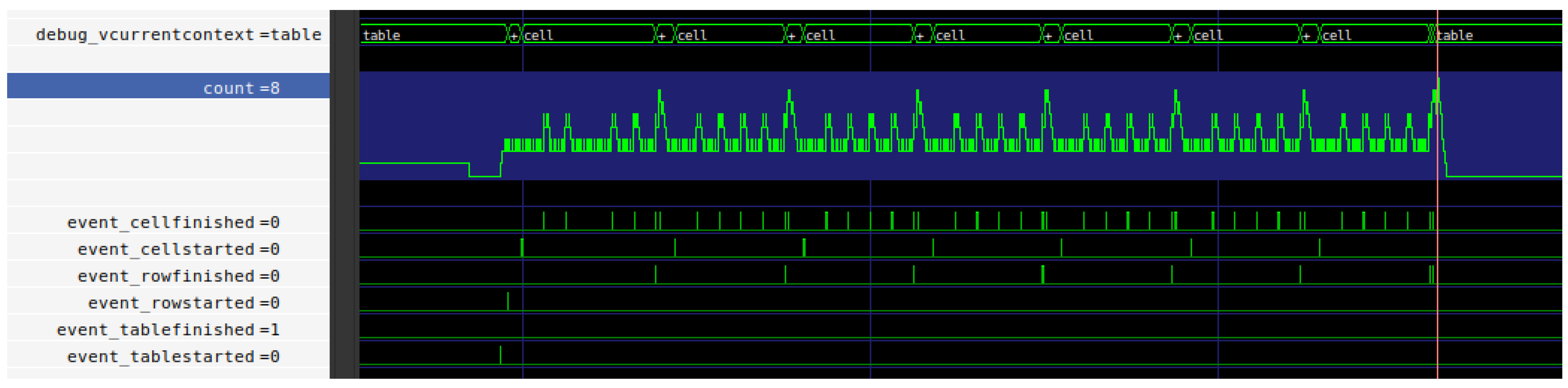
- Result The simulation results (Figure 8 represents one of the runs) show that the processing time for every additional chunk of payload is exactly 10 clock cycles, independent of the table schema. Memory usage grows exactly by the additional memory cell required to store each new chunk. The 4 × 4 table schema’s base execution time with one chunk per cell is 1263 clock cycles in our test (Table 1); the 3 × 4’s is 766 clock cycles (Table 2).
6.3. Synthesis Results
7. Comparison
7.1. Our Approach vs. Common Data Structures
7.2. Memory Consumption
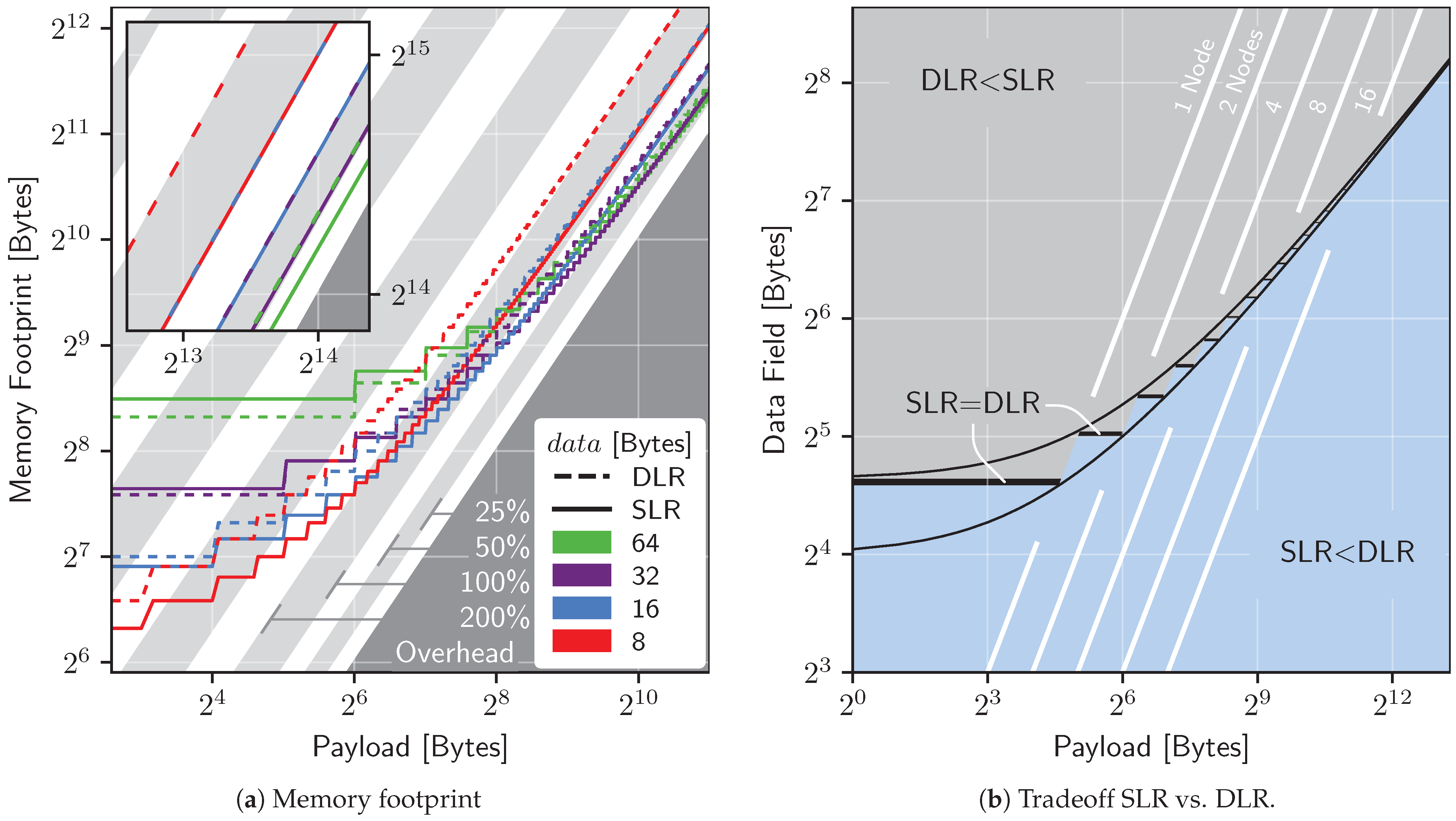
7.2.1. Singly vs. Doubly Linked Rings


7.2.2. Storing a Table
8. Conclusions
Further Ideas
Author Contributions
Funding
Data Availability Statement
Conflicts of Interest
Abbreviations
| BLOB | Binary Large Object |
| CPU | Central Processing Unit |
| CRUD | Create, Read, Update, Delete |
| DB | Database |
| DLR | Doubly-Linked Ring |
| DRAM | Dynamic Random Access Memory |
| FF | Flip-Flop |
| FPGA | Field Programmable Gate Array |
| FSM | Finite State Machine |
| HWDS | Hardware Data Structure |
| IOB | Input Output Block |
| LUT | Look-up table |
| RTDB | Real-Time Database |
| SLR | Singly-Linked Ring |
| SRAM | Static Random Access Memory |
| WCET | Worst-Case Execution Time |
Appendix A. Example Interface
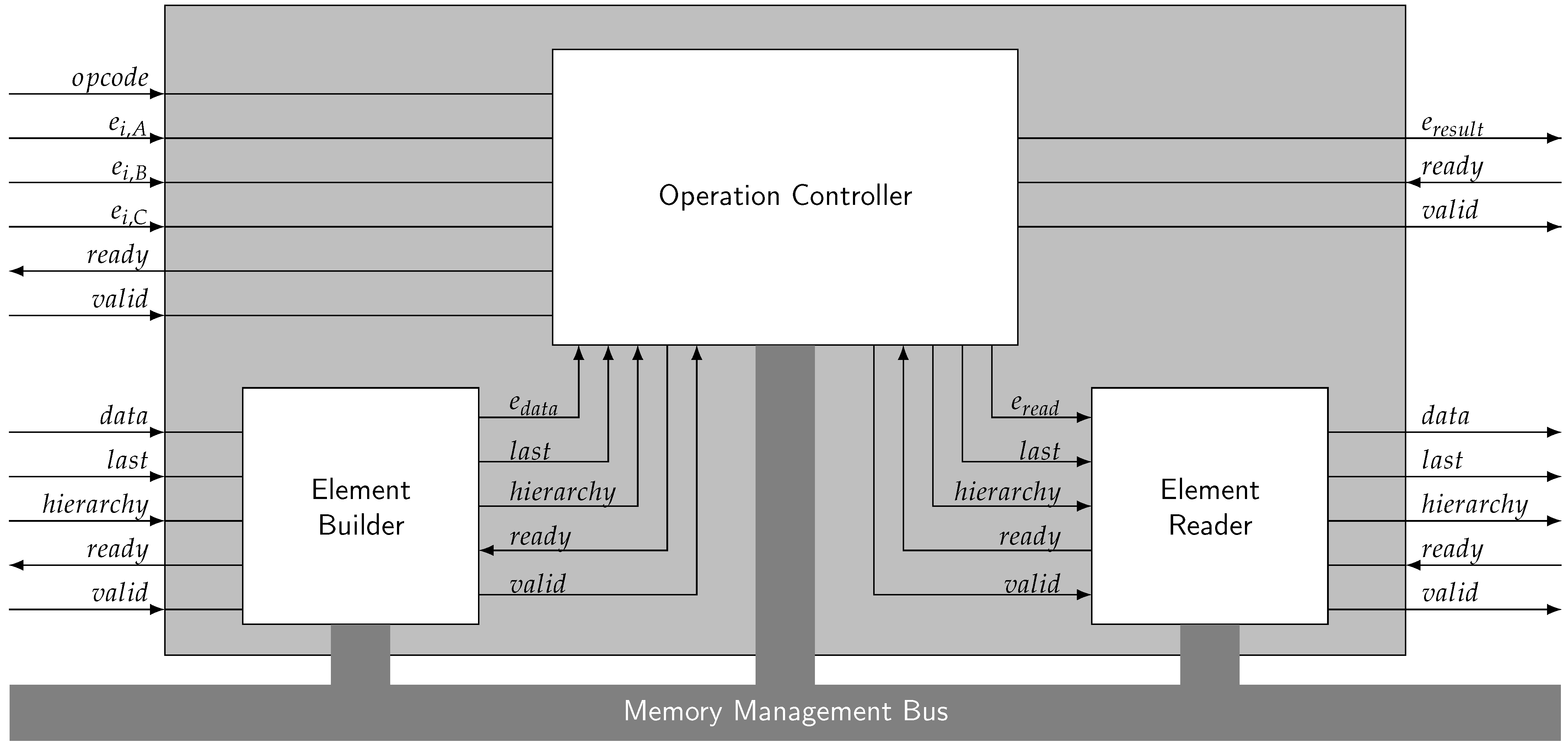
- Send for the to be replaced
- Send the data to the Element Builder
- Send the opcode for Update
- Send the data stream to the Element Builder via its , and inputs
- Set the input corresponding to to
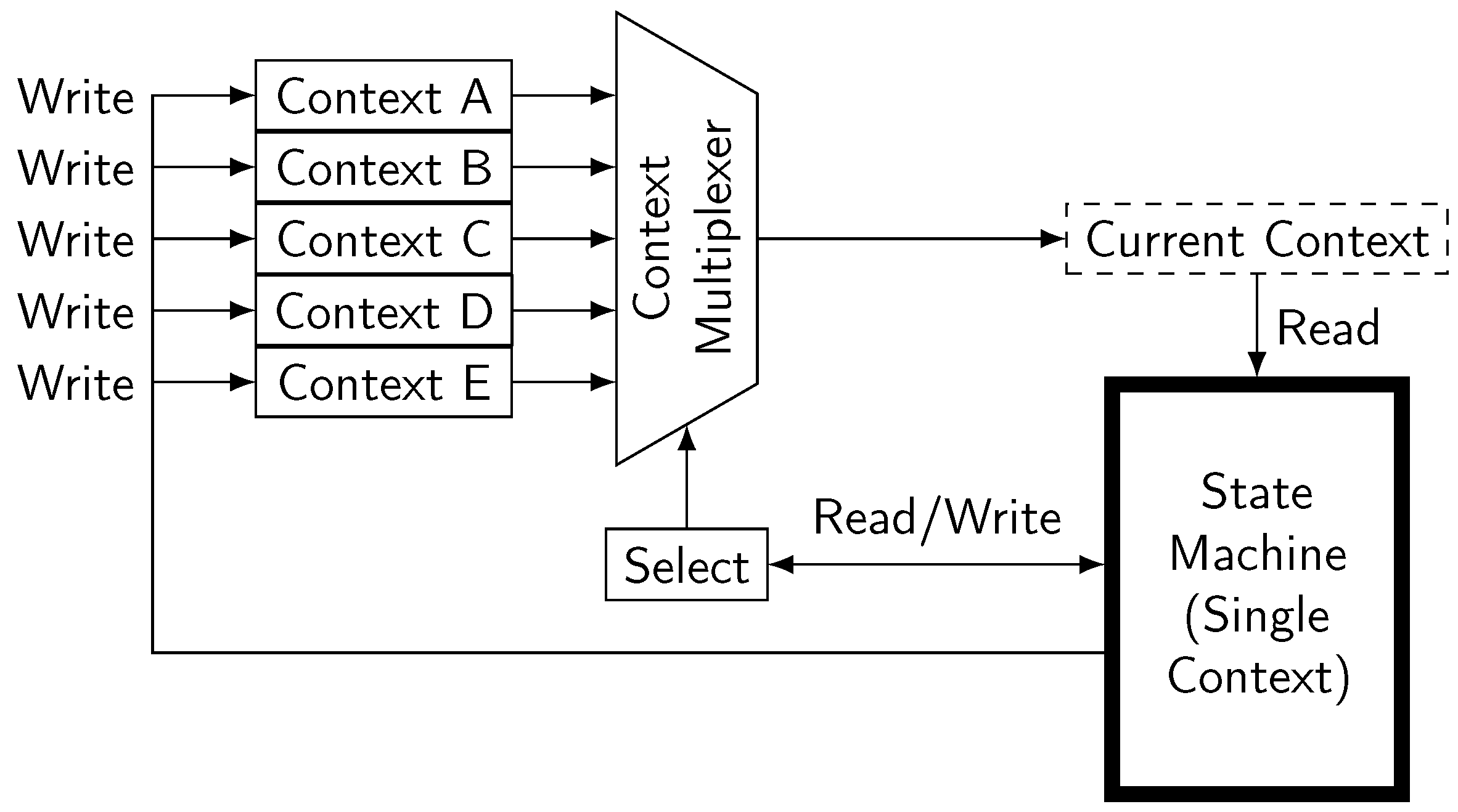
Appendix B. Synthesizable Implementation of Limited Depth Recursion

References
- Kao, B.; Garcia-Molina, H. An overview of real-time database systems. In Real Time Computing; Springer: Berlin/Heidelberg, Germany, 1994; pp. 261–282. [Google Scholar] [CrossRef]
- Ramamritham, K.; Sivasankaran, R.; Stankovic, J.; Towsley, D.; Xiong, M.; Haritsa, J.; Seshadri, S.; Kuo, T.W.; Mok, A.; Ulusoy, O.; et al. Advances in Real-Time Database Systems Research Special Section on RTDBS of ACM SIGMOD Record 25(1), March 1996; Boston University: Boston, MA, USA, 1996. [Google Scholar]
- Ramamritham, K.; Son, S.H.; DiPippo, L.C. Real-time databases and data services. Real-Time Syst. 2004, 28, 179–215. [Google Scholar] [CrossRef]
- Shanker, U.; Misra, M.; Sarje, A.K. Distributed real time database systems: Background and literature review. Distrib. Parallel Databases 2008, 23, 127–149. [Google Scholar] [CrossRef]
- Sha, L.; Rajkumar, R.; Lehooczky, J.P. Concurrency control for distributed real-time databases. ACM SIGMOD Rec. 1988, 17, 82–98. [Google Scholar] [CrossRef]
- Xiong, M.; Sivasankaran, R.; Stankovic, J.A.; Ramamritham, K.; Towsley, D. Scheduling Access to Temporal Data in Real-Time Databases. In Real-Time Database Systems; Springer: Boston, MA, USA, 1997. [Google Scholar] [CrossRef]
- Haritsa, J.R.; Livny, M.; Carey, M.J. Earliest Deadline Scheduling for Real-Time Database Systems. In Proceedings of the Real-Time Systems Symposium—1991, San Antonio, TX, USA, 4–6 December 1991; IEEE Computer Society: Washington, DC, USA, 1991; pp. 232–242. [Google Scholar] [CrossRef]
- Hong, D.; Johnson, T.; Chakravarthy, S. Real-time transaction scheduling: A cost conscious approach. In Proceedings of the 1993 ACM SIGMOD International Conference on Management of Data (SIGMOD ’93), Washington, DC, USA, 25–28 May 1993; pp. 197–206. [Google Scholar] [CrossRef]
- Lam, K.W.; Lee, V.C.S.; Hung, S.l. Transaction Scheduling in Distributed Real-Time Systems. Real-Time Syst. 2000, 19, 169. [Google Scholar] [CrossRef]
- Kuo, T.; Lam, K. Real-Time Database Systems: An Overview of System Characteristics and Issues. In Real-Time Database Systems; Springer: Boston, MA, USA, 2001; pp. 3–8. [Google Scholar] [CrossRef]
- Agrawal, D.; Abbadi, A.E.; Jeffers, R. Using delayed commitment in locking protocols for real-time databases. In Proceedings of the 1992 ACM SIGMOD International Conference on Management of Data (SIGMOD ’92), San Diego, CA, USA, 2–5 June 1992; pp. 104–113. [Google Scholar] [CrossRef]
- Son, S.H.; David, R.; Thuraisingham, B.M. Improving Timeliness in Real-Time Secure Database Systems. SIGMOD Rec. 1996, 25, 29–33. [Google Scholar] [CrossRef]
- Lam, K.Y.; Hung, S.L.; Son, S.H. On Using Real-Time Static Locking Protocols for Distributed Real-Time Databases. Real-Time Syst. 1997, 13, 141–166. [Google Scholar] [CrossRef]
- Park, C.; Park, S.; Son, S.H. Multiversion Locking Protocol with Freezing for Secure Real-Time Database Systems. IEEE Trans. Knowl. Data Eng. 2002, 14, 1141–1154. [Google Scholar] [CrossRef]
- Kim, J.; Kim, Y.; You, H.; Kim, J.; Ok, S. Design and Implementation of a Real-Time Static Locking Protocol for Main-Memory Database Systems. In Advances in Information Systems, Proceedings of the Third International Conference, ADVIS 2004, Izmir, Turkey, 20–22 October 2004; Yakhno, T.M., Ed.; Lecture Notes in Computer Science; Proceedings; Springer: Berlin/Heidelberg, Germany, 2004; Volume 3261, pp. 353–362. [Google Scholar] [CrossRef]
- Mittal, A.; Dandamudi, S.P. Dynamic versus Static Locking in Real-Time Parallel Database Systems. In Proceedings of the 18th International Parallel and Distributed Processing Symposium (IPDPS 2004), CD-ROM/Abstracts Proceedings, Santa Fe, NM, USA, 26–30 April 2004; IEEE Computer Society: Washington, DC, USA, 2004. [Google Scholar] [CrossRef]
- Wong, J.S.K.; Mitra, S. A nonblocking timed atomic commit protocol for distributed real-time database systems. J. Syst. Softw. 1996, 34, 161–170. [Google Scholar] [CrossRef]
- Lortz, V.B.; Shin, K.G.; Kim, J. MDARTS: A Multiprocessor Database Architecture for Hard Real-Time Systems. IEEE Trans. Knowl. Data Eng. 2000, 12, 621–644. [Google Scholar] [CrossRef]
- Nyström, D.; Tesanovic, A.; Norström, C.; Hansson, J. Database Pointers: A Predictable Way of Manipulating Hot Data in Hard Real-Time Systems. In Real-Time and Embedded Computing Systems and Applications, Proceedings of the 9th International Conference, RTCSA 2003, Tainan, Taiwan, 18–20 February 2003; Chen, J., Hong, S., Eds.; Lecture Notes in Computer Science; Revised Papers; Springer: Berlin/Heidelberg, Germany, 2003; Volume 2968, pp. 454–465. [Google Scholar] [CrossRef]
- Nogiec, J.M.; Desavouret, E. RTDB: A Memory Resident Real-Time Object Database; Fermi National Accelerator Lab. (FNAL): Batavia, IL, USA, 2003. [Google Scholar]
- Goebl, M.; Farber, G. A Real-Time-capable Hard-and Software Architecture for Joint Image and Knowledge Processing in Cognitive Automobiles. In Proceedings of the 2007 IEEE Intelligent Vehicles Symposium, Istanbul, Turkey, 13–15 June 2007; pp. 734–740. [Google Scholar] [CrossRef]
- Goebl, M. KogMo-RTDB: Einfuehrung in die Realzeitdatenbasis fuer Kognitive Automobile (C3) [KogMo-RTDB: Introduction to the Real-Time Data Base for Cognitive Automobiles]; Lehrstuhl für Realzeit-Computersysteme; Technische Universität München: München, Germany, 2007; Version 529+; Available online: https://www.kogmo-rtdb.de/download/docs/KogMo-RTDB_Einfuehrung.pdf (accessed on 21 July 2023).
- McObject. McObject Reaches out with a True Real-Time Deterministic Database for embOS RTOS Applications. Press Release. 2021. Available online: https://www.mcobject.com/press/deterministic-database-for-embos-rtos-applications/ (accessed on 31 January 2022).
- McObject. McObject Collaborates with Wind River to Deliver First-Ever Deterministic Database System for VxWorks-based Real-Time Embedded Systems. Press Release. 2021. Available online: https://www.mcobject.com/press/database-system-for-vxworks-rtos/ (accessed on 31 January 2022).
- Mueller, R.; Teubner, J. FPGA: What’s in It for a Database? In Proceedings of the 2009 ACM SIGMOD International Conference on Management of Data (SIGMOD ’09), Providence, RI, USA, 29 June–2 July 2009; pp. 999–1004. [Google Scholar] [CrossRef]
- Becher, A.; G., L.B.; Broneske, D.; Drewes, T.; Gurumurthy, B.; Meyer-Wegener, K.; Pionteck, T.; Saake, G.; Teich, J.; Wildermann, S. Integration of FPGAs in Database Management Systems: Challenges and Opportunities. Datenbank-Spektrum 2018, 18, 145–156. [Google Scholar] [CrossRef]
- Becher, A.; Ziener, D.; Meyer-Wegener, K.; Teich, J. A co-design approach for accelerated SQL query processing via FPGA-based data filtering. In Proceedings of the 2015 International Conference on Field Programmable Technology, FPT 2015, Queenstown, New Zealand, 7–9 December 2015; IEEE: Piscataway, NJ, USA, 2015; pp. 192–195. [Google Scholar] [CrossRef]
- Ziener, D.; Bauer, F.; Becher, A.; Dennl, C.; Meyer-Wegener, K.; Schürfeld, U.; Teich, J.; Vogt, J.S.; Weber, H. FPGA-Based Dynamically Reconfigurable SQL Query Processing. ACM Trans. Reconfig. Technol. Syst. 2016, 9, 25:1–25:24. [Google Scholar] [CrossRef]
- Sidler, D.; István, Z.; Owaida, M.; Alonso, G. Accelerating Pattern Matching Queries in Hybrid CPU-FPGA Architectures. In Proceedings of the 2017 ACM International Conference on Management of Data (SIGMOD ’17), Chicago, IL, USA, 14–19 May 2017; pp. 403–415. [Google Scholar] [CrossRef]
- Lekshmi, B.G.; Becher, A.; Meyer-Wegener, K.; Wildermann, S.; Teich, J. SQL Query Processing Using an Integrated FPGA-based Near-Data Accelerator in ReProVide. In Proceedings of the 23rd International Conference on Extending Database Technology, EDBT 2020, Copenhagen, Denmark, 30 March–2 April 2020; Bonifati, A., Zhou, Y., Salles, M.A.V., Böhm, A., Olteanu, D., Fletcher, G.H.L., Khan, A., Yang, B., Eds.; OpenProceedings: Konstanz, Germany, 2020; pp. 639–642. [Google Scholar] [CrossRef]
- Müller, R.; Teubner, J.; Alonso, G. Streams on Wires—A Query Compiler for FPGAs. Proc. VLDB Endow. 2009, 2, 229–240. [Google Scholar] [CrossRef]
- Müller, R.; Teubner, J.; Alonso, G. Glacier: A query-to-hardware compiler. In Proceedings of the ACM SIGMOD International Conference on Management of Data, SIGMOD 2010, Indianapolis, IN, USA, 6–10 June 2010; Elmagarmid, A.K., Agrawal, D., Eds.; ACM: New York, NY, USA, 2010; pp. 1159–1162. [Google Scholar] [CrossRef]
- Sukhwani, B.; Min, H.; Thoennes, M.; Dube, P.; Brezzo, B.; Asaad, S.; Dillenberger, D.E. Database Analytics: A Reconfigurable-Computing Approach. IEEE Micro 2014, 34, 19–29. [Google Scholar] [CrossRef]
- Sukhwani, B.; Thoennes, M.; Min, H.; Dube, P.; Brezzo, B.; Asaad, S.; Dillenberger, D. A Hardware/Software Approach for Database Query Acceleration with FPGAs. Int. J. Parallel Program. 2015, 43, 1129. [Google Scholar] [CrossRef]
- Dennl, C.; Ziener, D.; Teich, J. On-the-fly Composition of FPGA-Based SQL Query Accelerators Using a Partially Reconfigurable Module Library. In Proceedings of the 2012 IEEE 20th Annual International Symposium on Field-Programmable Custom Computing Machines, FCCM 2012, Toronto, ON, Canada, 29 April–1 May 2012; IEEE Computer Society: Washington, DC, USA, 2012; pp. 45–52. [Google Scholar] [CrossRef]
- Bayer, R.; McCreight, E.M. Organization and Maintenance of Large Ordered Indices. Acta Inform. 1972, 1, 173–189. [Google Scholar] [CrossRef]
- Fotakis, D.; Pagh, R.; Sanders, P.; Spirakis, P.G. Space Efficient Hash Tables with Worst Case Constant Access Time. In STACS 2003, Proceedings of the 20th Annual Symposium on Theoretical Aspects of Computer Science, Berlin, Germany, 27 February –1 March 2003; Alt, H., Habib, M., Eds.; Lecture Notes in Computer Science; Proceedings; Springer: Berlin/Heidelberg, Germany, 2003; Volume 2607, pp. 271–282. [Google Scholar] [CrossRef]
- Bloom, G.; Parmer, G.; Narahari, B.; Simha, R. Shared hardware data structures for hard real-time systems. In Proceedings of the 12th International Conference on Embedded Software, EMSOFT 2012, Part of the Eighth Embedded Systems Week, ESWeek 2012, Tampere, Finland, 7–12 October 2012; Jerraya, A., Carloni, L.P., Maraninchi, F., Regehr, J., Eds.; ACM: New York, NY, USA, 2012; pp. 133–142. [Google Scholar] [CrossRef]
- Moon, S.; Shin, K.G.; Rexford, J. Scalable Hardware Priority Queue Architectures for High-Speed Packet Switches. In Proceedings of the 3rd IEEE Real-Time Technology and Applications Symposium, RTAS ’97, Montreal, QC, Canada, 9–11 June 1997; IEEE Computer Society: Washington, DC, USA, 1997; pp. 203–212. [Google Scholar] [CrossRef]
- Kohutka, L.; Stopjakova, V. Rocket Queue: New data sorting architecture for real-time systems. In Proceedings of the 2017 IEEE 20th International Symposium on Design and Diagnostics of Electronic Circuits & Systems (DDECS), Dresden, Germany, 19–21 April 2017. [Google Scholar] [CrossRef]
- Kohutka, L.; Stopjakova, V. A new efficient sorting architecture for real-time systems. In Proceedings of the 2017 6th Mediterranean Conference on Embedded Computing (MECO), Bar, Montenegro, 11–15 June 2017. [Google Scholar] [CrossRef]
- Burleson, W.P.; Ko, J.; Niehaus, D.; Ramamritham, K.; Stankovic, J.A.; Wallace, G.; Weems, C.C. The spring scheduling coprocessor: A scheduling accelerator. IEEE Trans. Very Large Scale Integr. Syst. 1999, 7, 38–47. [Google Scholar] [CrossRef]
- Cameron, R.D.; Lin, D. Architectural support for SWAR text processing with parallel bit streams: The inductive doubling principle. In Proceedings of the 14th International Conference on Architectural Support for Programming Languages and Operating Systems, ASPLOS 2009, Washington, DC, USA, 7–11 March 2009; Soffa, M.L., Irwin, M.J., Eds.; ACM: New York, NY, USA, 2009; pp. 337–348. [Google Scholar] [CrossRef]
- ARM. AMBA AXI and ACE Protocol Specification; Standard; ARM: Cambridge, UK, 2013. [Google Scholar]
- Du, Z.; Zhang, Q.; Lin, M.; Li, S.; Li, X.; Ju, L. A Comprehensive Memory Management Framework for CPU-FPGA Heterogenous SoCs. IEEE Trans. Comput. Aided Des. Integr. Circuits Syst. 2023, 42, 1058–1071. [Google Scholar] [CrossRef]
- Dessouky, G.; Klaiber, M.J.; Bailey, D.G.; Simon, S. Adaptive Dynamic On-chip Memory Management for FPGA-based reconfigurable architectures. In Proceedings of the 24th International Conference on Field Programmable Logic and Applications, FPL 2014, Munich, Germany, 2–4 September 2014; IEEE: Piscataway, NJ, USA, 2014; pp. 1–8. [Google Scholar] [CrossRef]
- Trzepinski, M.; Skowron, K.; Korona, M.; Rawski, M. FPGA Implementation of Memory Management for Multigigabit Traffic Monitoring. In Man-Machine Interactions 5, Proceedings of the 5th International Conference on Man-Machine Interactions, ICMMI 2017, Kraków, Poland, 3–6 October 2017; Gruca, A., Czachórski, T., Harezlak, K., Kozielski, S., Piotrowska, A., Eds.; Advances in Intelligent Systems and Computing; Springer: Cham, Switzerland, 2017; Volume 659, pp. 555–565. [Google Scholar] [CrossRef]
- Kohútka, L.; Nagy, L.; Stopjaková, V. Low Latency Hardware-Accelerated Dynamic Memory Manager for Hard Real-Time and Mixed-Criticality Systems. In Proceedings of the 22nd IEEE International Symposium on Design and Diagnostics of Electronic Circuits & Systems, DDECS 2019, Cluj-Napoca, Romania, 24–26 April 2019; IEEE: Piscataway, NJ, USA, 2019; pp. 1–6. [Google Scholar] [CrossRef]
- Kohútka, L.; Nagy, L.; Stopjaková, V. Hardware Dynamic Memory Manager for Hard Real-Time Systems. Ann. Emerg. Technol. Comput. (AETiC) 2019, 3, 48–70. [Google Scholar] [CrossRef]
- Lohmann, S.; Tutsch, D. Hard Real-Time Memory-Management in a Single Clock Cycle (on FPGAs). In ECHTZEIT 2020, Proceedings of the Conference on Real-Time, Virtual Conference, 20 November 2020; Informatik Aktuell; Unger, H., Ed.; Springer: Wiesbaden, Germany, 2021; pp. 31–40. [Google Scholar] [CrossRef]
- ARM. AMBA 4 AXI4-Stream Protocol; Version 1.0; ARM IHI 0051A; ARM: Cambridge, UK, 2010. [Google Scholar]
- Okasaki, C. Purely Functional Random-Access Lists. In Proceedings of the Conference on Functional Programming Languages and Computer Architecture, La Jolla, CA, USA, 26–28 June 1995; ACM Press: New York, NY, USA, 1995; pp. 86–95. [Google Scholar] [CrossRef]


| Focused Cell Size | Execution Time | Memory |
|---|---|---|
| [Memory Cells] | [Clock Cycles] | [Memory Cells] |
| 1 | 1263 | 121 |
| 2 | 1273 | 122 |
| 3 | 1283 | 123 |
| 4 | 1293 | 124 |
| 5 | 1303 | 125 |
| 6 | 1313 | 126 |
| 7 | 1323 | 127 |
| 8 | 1333 | 128 |
| Focused Cell Size | Execution Time | Memory |
|---|---|---|
| [Memory Cells] | [Clock Cycles] | [Memory Cells] |
| 1 | 766 | 74 |
| 2 | 776 | 75 |
| 3 | 786 | 76 |
| 4 | 796 | 77 |
| 5 | 806 | 78 |
| 6 | 816 | 79 |
| 7 | 826 | 80 |
| 8 | 836 | 81 |
| Outstanding Transactions Allowed | Synthesis & Implementation Strategy | Achieved Frequency [MHz] | Worst Negative Slack [ns] | LUT | FF |
|---|---|---|---|---|---|
| 2 | Performance | 166.7 | 0.037 | 3603 | 1487 |
| 2 | Area | 178.6 | 0.000 | 2722 | 1389 |
| 7 | Performance | 161.3 | 0.012 | 3783 | 1501 |
| 7 | Area | 169.5 | 0.005 | 2738 | 1407 |
| 15 | Performance | 153.8 | 0.044 | 3720 | 1520 |
| 15 | Area | 152.7 | 0.025 | 2801 | 1426 |
Disclaimer/Publisher’s Note: The statements, opinions and data contained in all publications are solely those of the individual author(s) and contributor(s) and not of MDPI and/or the editor(s). MDPI and/or the editor(s) disclaim responsibility for any injury to people or property resulting from any ideas, methods, instructions or products referred to in the content. |
© 2023 by the authors. Licensee MDPI, Basel, Switzerland. This article is an open access article distributed under the terms and conditions of the Creative Commons Attribution (CC BY) license (https://creativecommons.org/licenses/by/4.0/).
Share and Cite
Lohmann, S.; Tutsch, D. The Doubly Linked Tree of Singly Linked Rings: Providing Hard Real-Time Database Operations on an FPGA. Computers 2024, 13, 8. https://doi.org/10.3390/computers13010008
Lohmann S, Tutsch D. The Doubly Linked Tree of Singly Linked Rings: Providing Hard Real-Time Database Operations on an FPGA. Computers. 2024; 13(1):8. https://doi.org/10.3390/computers13010008
Chicago/Turabian StyleLohmann, Simon, and Dietmar Tutsch. 2024. "The Doubly Linked Tree of Singly Linked Rings: Providing Hard Real-Time Database Operations on an FPGA" Computers 13, no. 1: 8. https://doi.org/10.3390/computers13010008
APA StyleLohmann, S., & Tutsch, D. (2024). The Doubly Linked Tree of Singly Linked Rings: Providing Hard Real-Time Database Operations on an FPGA. Computers, 13(1), 8. https://doi.org/10.3390/computers13010008