Article

Batch Gradient Learning Algorithm with Smoothing L1 Regularization for Feedforward Neural Networks

by
Khidir Shaib Mohamed
1,2
1
Department of Mathematics, College of Sciences and Arts in Uglat Asugour, Qassim University, Buraydah 51452, Saudi Arabia
2
Department of Mathematics and Computer, College of Science, Dalanj University, Dilling P.O. Box 14, Sudan
Computers 2023, 12(1), 4; https://doi.org/10.3390/computers12010004
Submission received: 6 December 2022 / Revised: 13 December 2022 / Accepted: 16 December 2022 / Published: 23 December 2022

Abstract

:
Regularization techniques are critical in the development of machine learning models. Complex models, such as neural networks, are particularly prone to overfitting and to performing poorly on the training data. L 1 regularization is the most extreme way to enforce sparsity, but, regrettably, it does not result in an NP-hard problem due to the non-differentiability of the 1-norm. However, the L 1 regularization term achieved convergence speed and efficiency optimization solution through a proximal method. In this paper, we propose a batch gradient learning algorithm with smoothing L 1 regularization (BGS L 1 ) for learning and pruning a feedforward neural network with hidden nodes. To achieve our study purpose, we propose a smoothing (differentiable) function in order to address the non-differentiability of L 1 regularization at the origin, make the convergence speed faster, improve the network structure ability, and build stronger mapping. Under this condition, the strong and weak convergence theorems are provided. We used N-dimensional parity problems and function approximation problems in our experiments. Preliminary findings indicate that the BGS L 1 has convergence faster and good generalization abilities when compared with BG L 1 / 2 , BG L 1 , BG L 2 , and BGS L 1 / 2 . As a result, we demonstrate that the error function decreases monotonically and that the norm of the gradient of the error function approaches zero, thereby validating the theoretical finding and the supremacy of the suggested technique.

1. Introduction

Artificial neural networks (ANNs) are computational networks based on biological neural networks. These networks form the basis of the human brain’s structure. Similar to neurons in a human brain, ANNs also have neurons that are interconnected to one another through a variety of layers. These neurons are known as nodes. The human brain is made up of 86 billion nerve cells known as neurons. They are linked to 1000 s of other cells by axons. Dendrites recognize stimulation from the external environment as well as inputs from sensory organs. These inputs generate electric impulses that travel quickly through the neural network. A neuron can then forward the message to another neuron to address the issue or not forward it at all. ANNs are made up of multiple nodes that mimic biological neurons in the human brain (See Figure 1). A feedforward neural network (FFNN) is the first and simplest type of ANN, and now it contributes significantly and directly to our daily lives in a variety of fields, such as education tools, health conditions, economics, sports, and chemical engineering [1,2,3,4,5].
The most widely used learning strategy in FFNNs is the backpropagation method [6]. There are two methods for training the weights: batch and online [7,8]. In the batch method, the weights are modified after each training pattern is presented to the network, whereas in the online method, the error is accumulated during an epoch and the weights are modified after the entire training set is presented.
Overfitting in mathematical modeling is the creation of an analysis that is precisely tailored to a specific set of data and, thus, may fail to fit additional data or predict future findings accurately [9,10]. An overfitted model is one that includes more parameters than can be justified by the data [11]. Several techniques, such as cross-validation [12], early stopping [13], dropout [14], regularization [15], big data analysis [16], or Bayesian regularization [17], are used to reduce the amount of overfitting.
Regularization methods are frequently used in the FFNN training procedure and have been shown to be effective in improving generalization performance and decreasing the magnitude of network weights [18,19,20]. A term proportional to the magnitude of the weight vector is one of the simplest regularization penalty terms added to the standard error function [21,22]. Many successful applications have used various regularization terms, such as weight decay [23], weight elimination [24], elastic net regularization [25], matrix regularization [26], and nuclear norm regularization [27].
Several regularization terms are made up of the weights, resulting in the following new error function:
E W = E ˇ W + λ W q q  
where E ˇ w is the standard error function depending on the weights w , λ is the regularization parameter, and · q is the q-norm is given by
W q = w 1 q + w 2 q + + w N q 1 q
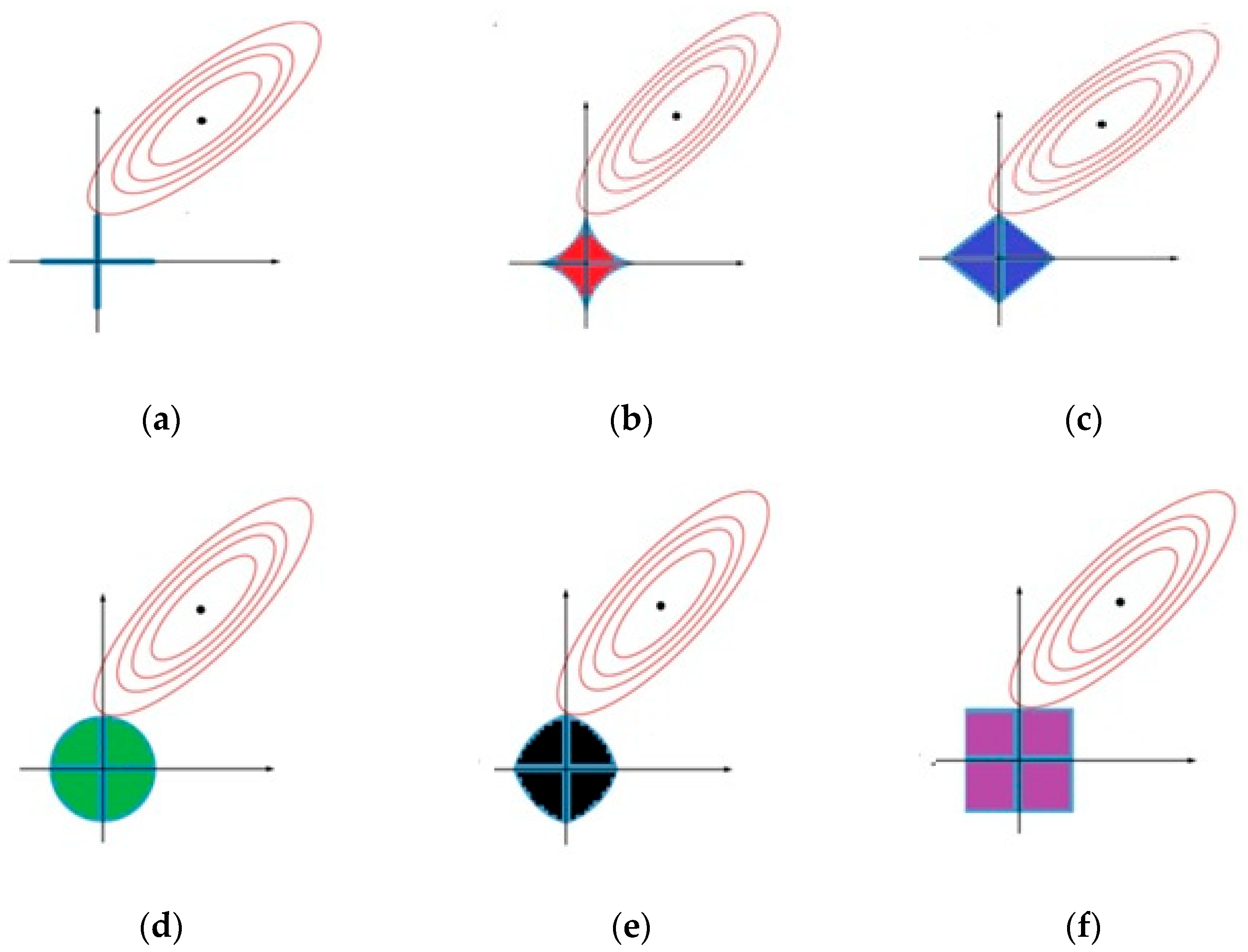
where ( 0 q 2 ). The gradient descent algorithm is a popular method for solving this type of problem (1). The graphics of the L 0 , L 1 / 2 , L 1 , L 2 , elastic net, and L regularizers in Figure 2 show the sparsity. The sparsity solution, as shown in Figure 2, is the first point at which the contours touch the constraint region, and this will coincide with a corner corresponding to a zero coefficient. It is obvious that the L 1 regularization solution occurs at a corner with a higher possibility, implying that it is sparser than the others. The goal of network training is to find W so that E W = min E W . The weight vectors’ corresponding iteration formula is
W n e w = W η d E W d W  
L 0 regularization has a wide range of applications in sparse optimization [28]. As the L 0 regularization technique is an NP-hard problem, optimization algorithms, such as the gradient method, cannot be immediately applied [29]. To address this issue, ref. [30] proposes smoothing L 0 regularization with the gradient method for training FFNN. According to the regularization concept, Lasso regression was proposed to obtain the sparse solution based on L 1 regularization to reduce the complexity of the mathematical model [31]. Lasso quickly evolved into a wide range of models due to its outstanding performance. To achieve maximally sparse networks with minimal performance degradation, neural networks with smoothed Lasso regularization were used [32]. Due to its oracle properties, sparsity, and unbiasedness, the L 1 / 2 regularizer has been widely utilized in various studies [33]. A novel method for forcing neural network weights to become sparser was developed by applying L 1 / 2 regularization to the error function [34]. L 2 regularization is one of the most common types of regularization since the 2-norm is differentiable and learning can be advanced using a gradient method [35,36,37,38]; with L 2 regularization, the weights provided are bounded [37,38]. As a result, L 2 regularization is useful for dealing with overfitting problems.
Figure 2. The sparsity property of different regularization (a) L 0 regularization, (b) L 1 / 2 regularization, (c) L 1 regularization, (d) L 2 regularization, (e) elastic net regularization, (f) L regularization.
Computers 12 00004 g002
The batch update rule, which modifies all weights in each estimation process, has become the most prevalent. As a result, in this article, we concentrated on the gradient method with a batch update rule and smoothing L 1 regularization for FFNN. We first show that if certain Propositions 1–3 are met, the error sequence will be uniformly monotonous, and the algorithm will be weakly convergent during training. Secondly, if there are no interior points in the error function, the algorithm with weak convergence is strongly convergent with the help of Proposition 4. Furthermore, numerical experiments demonstrate that our proposed algorithm eradicates oscillation and increases the computation learning algorithm better than the standard L 1 / 2 regularization, L 1 regularization, L 2 regularization, and even the smoothing L 1 / 2 regularization methods.
The following is the rest of this paper. Section 2 discusses FFNN, the batch gradient method with L 1 regularization (BG L 1 ), and the batch gradient method with smoothing L 1 regularization (BGS L 1 ). The materials and methods are given in Section 3. Section 4 displays some numerical simulation results that back up the claims made in Section 3. Section 5 provides a brief conclusion. The proof of the convergence theorem is provided in “Appendix A”.

2. Network Structure and Learning Algorithm Methodology

2.1. Network Structure

A three-layer neural network based on error back-propagation is presented. Consider a three-layer structures consisting of N input layers, M hidden layers and 1 output layer. Given that g   :     can be a transfer function for the hidden and output layers, this is typically, but not necessarily, a sigmoid function. Let w 0 = w 01 , w 02 , , w 0 M T M be the weight vector between all the hidden layers and the output layer, and let denoted w j = w j 1 , w j 2 , , w j N T N be the weight vector between all the input layers and the hidden layer j j = 1 , 2 , , M . To classify the offer, we write all the weight parameters in a compact form, i.e., W = w 0 T , w 1 T , , w M T M + N M , and we have also given a matrix V = w 1 , w 2 , , w M T M N × M . Furthermore, we define a vector function
F x = f ( x 1 , f ( x 2 ) , , f ( x N ) ) T
where x = ( x 1 , x 2 , , x N ) T N . For any given input ξ M the output of the hidden neuron is F V   ξ , and the final output of the network is
y = f w 0 · F V   ξ
where w 0 · F V   ξ represents the inner product between the vectors w 0 and F V   ξ .

2.2. Modified Error Function with Smoothing L 1 Regularization (BGS L 1 )

Given that the training set is { ξ l , O l } l = 1 L   N × , where O l is the desired ideal output for the input ξ l . The standard error function E W without regularization term as following
E ˇ W = 1 2 l = 1 L O l f w 0 · F V ξ l 2 = l = 1 L f l w 0 · F V ξ l  
where f l t 1 2 O l f l t 2 . Furthermore, the gradient of the error function is given by
E ˇ w 0 W = l = 1 L f l w 0 · F V ξ l F V ξ l  
E ˇ w j W = l = 1 L f l w 0 · F V ξ l w 0 l f l w j · ξ l ξ l  
The modified error function E W with L 1 regularization is given by
E W = E ˇ W + λ j = 1 M w j  
where W   denoted the absolute value of the weights. The purpose of the network training is to find W such that
E   W = m i n E   W  
The gradient method is a popular solution for this type of problem. Since Equation (8) involves the absolute value, this is a combinatorial optimization problem, and the gradient method cannot be employed to immediately minimize such an optimization problem. However, in order to estimate the absolute value of the weights, we recognize the use of a continuous and differentiable function to replace L 1 regularization by smoothing in (8). The error function with smoothing L 1 regularization can then be adapted by
E W = E ˇ W + λ j = 1 M h w j ,  
where h x is any continuous and differentiable functions. Specifically, we use the following piecewise polynomial function as:
h t =   t     i f   t m 1 8 m 3 t 4 + 3 4 m t 2 + 3 8 m   ,   i f     t < m ,    
where m is a suitable constant. Then the gradient of the error function is given by
E W W = ( E w 0 T W ,   E w 1 T W   , E w 2 T W ,   ,   E w M T W ) T  
The gradient of the error function in (10) with respect to w j is given by
E w j W = E ˇ w j W + λ h w j  
The weights W k updated iteratively starting from an initial value W 0 by
W k + 1 = W k + Δ W k ,   k = 0 , 1 , 2 , ,
and
Δ w j k = η E ˇ w j k W + λ h w j k  
where η > 0   is learning rate, and λ is regularization parameter.

3. Materials and Methods

It will be necessary to prove the convergence theorem using the propositions below.
Proposition 1.
f t ,   f t ,   f t and F t ,   F t are uniformly bounded for t .
Proposition 2.
w 0 k   k = 0 , 1 , is uniformly bounded.
Proposition 3.
η and λ are chosen to satisfy: 0 < η < 1 / λ A C 1 , where
C 1 = L 1 + C 2 C 3 max C 2 , C 5 + 1 2 L 1 + C 2 C 3 + 1 2 L C 3 2 C 4 2 C 5 , C 2 = m a x B C 3 , C 3 C 4 2 , C 3 = max sup t f t , sup t f t ,   sup t f t , sup t , 1 l L f l t , sup t , 1 l L f l t , C 4 = min 1 l L ξ l ,   C 5 = sup k w 0 k .
Proposition 4.
There exists a closed bounded region Θ such that W k Θ , and set Θ 0 = W Θ :   E w W = 0 contains only finite points.
Remark 1.
Both the hidden layer and output layer have the same transfer function, is t a n s i g · . A uniformly bounded weight distribution is shown in Propositions 1 and 2. Thus, Proposition 4 is reasonable. The Equation (10) and Proposition 1, f l t ,   f l t ,   f l t are uniformly bounded for Proposition 3. Regarding Proposition 2, we would like to make the following observation. This paper focuses mainly on simulation problems with f t being a sigmoid function satisfying Proposition 1. Typically, simulation problems require outputs of 0 and 1, or −1 and 1. To control the magnitude of the weights w 0 , one can change the desired output into 0 + α and 1 − α, or −1 + α and 1 − α, respectively, where α > 0 is a small constant. Actually, a more important reason of doing so is to prevent the overtraining, cf. [39]. In the case of sigmoid functions, when f t is bounded, the weights for the output layer are bounded.
Theorem 1.
Let the weight W k be generated by the iteration algorithm (14) for an arbitrary initial value W 0 , the error function E W be defined by (10) and if propositions 1–3 are valid, then we have
I.
E W k + 1 E W k ,   k = 0 , 1 , ;
II.
There exists E 0 such that lim k E w j W k = E .
III.
lim k Δ W k = 0 ,
IV.
Further, if proposition 4 is also valid, we have the following strong convergence
V.
There exists a point W Θ 0 such that lim k W k = W .
Note: 
It is shown in conclusion (I) and (II) that the error function sequence E W k is monotonic and has a limit (II). According to conclusions (II) and (IV), E W k and E W W k are weakly converging. The strong convergence of { W k } is mentioned in Conclusion (V).
We used the following strategy as a neuron selection criterion by simply computing the norm of the overall outgoing weights from the neuron number to ascertain whether a neuron number in the hidden units will survive or be removed after training. There is no standard threshold value in the literature for eliminating redundant weighted connections and redundant neurons from the initially assumed structure of neural networks. The sparsity of the learning algorithm was measured using the number of weights with absolute values of ≤0.0099 and ≤0.01, respectively, according to ref. [40]. In this study, we chose 0.00099 as a threshold value at random, which is less than the existing thresholds in the literature. This procedure is repeated ten times. Algorithm 1 describes the experiment procedure.
Algorithm 1 The learning algorithm
InputInput the dimension M , the number N of the nodes, the number maximum iteration number K , the learning rate η , the regularization parameter λ , and the sample training set is { ξ l , O l } l = 1 L   N × .
InitializationInitialize randomly the initial weight vectors w 0 0 = ( w 0 , 1 0 , , w 0 , M 0 ) T M and w j 0 = ( w j 0 0 , , w j N 0 ) T N   j j = 1 , 2 , , M
TrainingFor k = 1 , 2 , , K do
Compute the error function Equation (10).
Compute the gradients Equation (15).
Update the weights w 0 0 and w j 0   1 j M by using Equation (14).
end
OutputOutput the final weight vectors w 0 K and w j K   1 j M

4. Experimental Results

The simulation results for evaluating the performance of the proposed BGS L 1 algorithm are presented in this section. We will compare BGS L 1 performance to that of four common regularization algorithms: the batch gradient method with L 1 / 2 regularization (BG L 1 / 2 ), the batch gradient method with smoothing L 1 / 2 regularization (BGS L 1 / 2 ), the batch gradient method with L 1 regularization (BG L 1 ), and the batch gradient method with L 2 regularization (BG L 2 ). Numerical experiments on the N-dimensional parity and function approximation problems support our theoretical conclusion.

4.1. N-Dimensional Parity Problems

The N-dimensional parity problem is another popular task that generates a lot of debate. If the input pattern contains an odd number of ones, the output criterion is one; alternatively, the output necessity is zero. An N-M-1 architecture (N inputs, M hidden nodes, and 1 output) is employed to overcome the N-bit parity problem. The well-known XOR problem is simply a 2-bit parity problem [41]. Here, the 3-bit and 6-bit parity problems are used as an example to test the performance of BGS L 1 . The network has three layers: input layers, hidden layers, and an output unit.
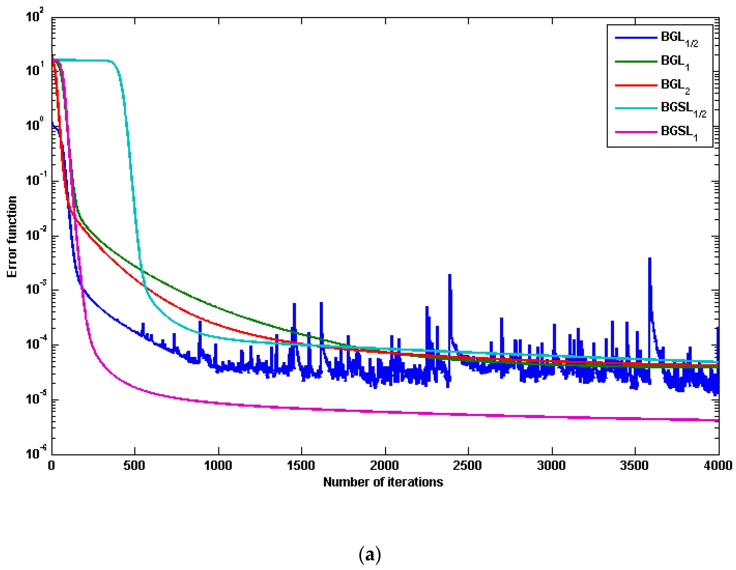
Table 1 shows the parameter settings for the corresponding network, where LR and RP are abbreviations for the learning rate and regularization parameter, respectively. Figure 3 and Figure 4 show the performance results of BG L 2 , BG L 1 , BG L 1 / 2 , BGS L 1 / 2 , and BGS L 1 for 3-bit and 6-bit parity problems, respectively. As illustrated by Theorem 1, the error function decreases monotonically in Figure 3a and Figure 4a, and the norm of the gradients of the error function approaches zero in Figure 3b and Figure 4b. According to the comparison results, our proposal demonstrated superior learning ability and faster convergence. This corresponds to our theoretical analysis. Table 2 displays the average error and running time of ten experiments, demonstrating that BGS L 1 not only converges faster but also has better generalization ability than others.

4.2. Function Approximation Problem

A nonlinear function has been devised to compare the approximation capabilities of the above algorithms:
G x = 1 2 x sin x  
where x 4 , 4 and chooses 101 training samples from an evenly spaced interval of [−4, 4]. The initial weight of the network is typically generated at random within a given interval; training begins with an initial point and gradually progresses to a minimum of error along the slope of the error function, which is chosen stochastically in [−0.5, 0.5]. The training parameters are as follows: 0.02 and 0.0005 represent the learning rate ( η ) and parameter regularization ( λ ), respectively. The stop criteria are set to 1000 training cycles.
The average error and norm of the gradient and running time of 10 experiments are presented in Table 3. Through the results obtained from Figure 5a,b, respectively, we see that BGS L 1 has a better mapping capability than BGS L 1 / 2 , BG L 1 / 2 , BG L 1 and BG L 2 , with the error decreasing monotonically as learning proceeds and its gradient go to zero. Table 3 shows the preliminary results are extremely encouraging and that the speedup and generalization ability of BGS L 1 is better than BGS L 1 / 2 , BG L 1 / 2 , BG L 1 and BG L 2 .

5. Discussion

Table 2 and Table 3, respectively, show the performance comparison of the average error and the average norms of gradients under our five methods over the 10 trials. Table 2 shows the results of N-dimensional parity problems using the same parameters, while Table 3 shows the results of function approximation problems using the same parameters.
The comparison convincing in Table 2 and Table 3 shows that the BGS L 1 is more efficient and has better sparsity-promoting properties than BG L 1 / 2 , BG L 1 , BG L 2 and even than the BGS L 1 / 2 . In addition to that, Table 2 and Table 3 show that our proposed algorithm is faster than that of all numerical results. L 1 / 2 regularization is sparser than the traditional L 1 regularization solution. Recently, in ref. [34], the BGS L 1 / 2 also shows that the sparsity is better than that of BG L 1 / 2 . The results of ref. [33] show that the L 1 / 2 regularization has been demonstrated to have the following properties: unbiasedness, sparsity, and oracle properties.
We obtained all three numerical results for five different methods using one hidden layer of FFNNs. Our new method proposed a sparsification technique for FFNNs can be extended to encompass any number of hidden layers.

6. Conclusions

L 1 regularization is thought to be an excellent pruning method for neural networks. L 1 regularization, on the other hand, is also an NP-hard problem. In this paper, we propose BGS L 1 , a batch gradient learning algorithm with smoothing L 1 regularization for training and pruning feedforward neural networks, and we approximate the L 1 regularization by smoothing function. We analyzed some weak and strong theoretical results under this condition, and the computational results validated the theoretical findings. The proposed algorithm has the potential to be extended to train neural networks. In the future, we will look at the case of the online gradient learning algorithm with a smoothing L 1 regularization term.

Funding

The researcher would like to thank the Deanship of Scientific Research, Qassim University for funding the publication of this project.

Data Availability Statement

All data has been presented in this paper.

Acknowledgments

The tresearcher would like to thank the referees for their careful reading and helpful comments.

Conflicts of Interest

The authors declare no conflict of interest.

Appendix A

To prove the strong convergence, we will use the following result, which is basically the same as Lemma 3 in [38]. So its proof is omitted.
Lemma A1.
Let F : Θ n be continuous for a bounded closed region Θ , and Θ 0 = z Θ : F z = 0 . The projection of Θ 0 on each coordinate axis does not contain any interior point. Let the sequence z k satisfy:
(a) 
lim k F z k = 0 ;
(b) 
lim k z k + 1 z k = 0 .
Then, there exists a unique z Θ 0 such that lim k z k = z .
There are four statements in the proof of Theorem 1, each one is shown in I IV . We use the following notations for convenience:
σ k = j = 0 M ( Δ w j k ) 2
From error function (10), we can write
E W k + 1 = 1 2 l = 1 L f l w 0 k + 1 · F V k + 1 ξ l + λ j = 0 M h ( w j k + 1 )  
and
E W k = 1 2 l = 1 L f l w 0 k · F ( V k ξ l ) + λ j = 0 M h ( w j k )  
Proof to (I) of Theorem 1.
Using the (A2), (A3), and Taylor expansion. We have
E W k + 1 E W k = l = 1 L f l w 0 k + 1 · F V k + 1 ξ l f l w 0 k · F V k ξ l + λ j = 0 M [ h ( w j k + 1 ) h ( w j k ) ] = j = 1 L f l w 0 n · F V k ξ l F w 0 n · V k + 1 ξ l F w 0 n · V k ξ l + λ j = 0 M h ( w j k ) + 1 2 h t k , j Δ w j k · Δ w j k + 1 2 l = 1 L f l s k , l w 0 k + 1 · F V k + 1 ξ l w 0 k · F V k ξ l 2 = l = 1 J f l w 0 k · F V k ξ l F V k ξ l Δ w 0 k + λ h w 0 k · Δ w 0 k + j = 1 L f l w 0 n · F V k ξ l F V k + 1 ξ l F V k ξ l · w 0 k + λ j = 1 M h ( w j k ) · Δ w j k + λ 2 h t k , j j = 0 M ( Δ w j k ) 2 + j = 1 L f l w 0 n · F V k ξ l F V k + 1 ξ l F V k ξ l · Δ w 0 k + 1 2 l = 1 L f l s k , l w 0 k + 1 · F V k + 1 ξ l w 0 k · F V k ξ l 2 1 η λ 2 h t k , j j = 0 M ( Δ w j k ) 2 + 1 2 l = 1 L f l s k , l w 0 k + 1 · F V k + 1 ξ l w 0 k · F V k ξ l 2 + l = 1 L f l w 0 k · F V k ξ l F V k + 1 ξ l F V k ξ l Δ w 0 n + 1 2 j = 1 M l = 1 L f l w 0 k · F V k ξ l w 0 j k f l t k , j , l ( Δ w j k · ξ l ) 2
where t k , l is between w 0 k + 1 · F V k + 1 ξ l and w 0 k · F V k ξ l and t k , j , l is between w j k + 1 · ξ l and w j k · ξ l . From (16), Proposition 1 and the Lagrange mean value theorem. We have
F V k + 1 ξ l F V k ξ l 2 = f w 1 k + 1 · ξ l f w 1 k · ξ l f w q k + 1 · ξ l f w q k · ξ l 2 = f t ˜ 1 , j , l w 1 k + 1 w 1 k · ξ l f t ˜ i , j , l w q k + 1 w q k · ξ l 2 C 2 j = 1 M ( Δ w j k ) 2    
and
F x B t f t C 2 ,  
where t ˜ k , j , l   1 i B is between w j k + 1 · ξ l and w j k · ξ l . According to Cauchy-Schwarz inequality, Proposition 1, (16), (A5) and (A6). We have
1 2 l = 1 L f l t k , l w 0 k + 1 · F V k + 1 ξ l w 0 k · F V k ξ l 2 C 2 2 l = 1 L w 0 k + 1 · F V k + 1 ξ l w 0 k · F V k ξ l 2 C 2 2 l = 1 L 2 C 2 2 Δ w 0 k + C 5 2 F V k + 1 ξ l F V k ξ l 2 C 6 l = 1 L Δ w 0 k 2 + C 2 j = 1 M ( Δ w j k ) 2 LC 6 1 + C 2 j = 0 M Δ w j k 2 C 7 j = 0 M ( Δ w j k ) 2 ,
where C 6 = C 2   m a x C 2 2 , C 5 2 and C 7 = L C 6 1 + C 2 . In the same way, we have
l = 1 L f l w 0 k · F V k ξ l F V k + 1 ξ l F V k ξ l Δ w 0 k   C 3 2 l = 1 L Δ w 0 k 2 + C 2 j = 1 M ( Δ w j k ) 2 1 2 L C 3 1 + C 2 j = 0 M ( Δ w j k ) 2 C 8 j = 0 M ( Δ w j k ) 2 ,
where C 8 = 1 2 L C 3 1 + C 2 . It follows from Propositions 1 and 2 that
1 2 j = 1 M l = 1 J f l w 0 k · F V k ξ l w 0 j k f j t k , j , l ( Δ w j k · ξ l ) 2 1 2 L C 3 2 C 4 2 C 5 j = 0 M ( Δ w j k ) 2 C 9 j = 0 M ( Δ w j k ) 2 ,
where C 9 = 1 2 L C 3 2 C 4 2 C 5 .
Let C 1 = C 7 + C 8 + C 9 .
A combination of (A4) to (A9), and from h x it easy to obtained h t 3 8 m , + , h t 1 ,   1 , h t 0 ,   3 2 m , and A ¯ = 3 / 2 ω . We have
E W k + 1 E W k [ 1 η λ 2 h t k , j ] j = 1 M ( Δ w j k ) 2 + C 1 j = 1 M ( Δ w j k ) 2 [ 1 η λ 2 A ¯ C 1 ] j = 1 M ( Δ w j k ) 2   0 .
Conclusion (I) of Theorem 1 is proved if the Proposition 3 is valid. □
Proof to (II) of Theorem 1.
Since the nonnegative sequence E W k is monotone and bounded below, there must be a limit value E < 0 such that
lim k E W k = E .
So conclusion (II) is proved. □
Proof to (III) of Theorem 1.
Proposition 1, (A10) and let μ > 0. We have
μ = 1 η λ A C 1  
Thus, we can write
E W k + 1 E W k μ ρ n E W 0 μ q = 0 n ρ n ,  
when E W k + 1 > 0 for any k 0 and set k   , then we have
q = 0 ρ n 1 μ E W 0 < .
This with (12), (14) and (A1). We have
lim k Δ W k = l i m k E w W k = 0  
Proof to (IV) of Theorem 1.
As a result, we can prove that the convergence is strong. Noting Conclusions (IV), we take x = W and h x = E z x . This together with the finiteness of Θ 0 (cf. Proposition 4), (A13), and Lemma 1 leads directly to conclusion (IV). This completes the proof. □

References

  1. Deperlioglu, O.; Kose, U. An educational tool for artificial neural networks. Comput. Electr. Eng. 2011, 37, 392–402. [Google Scholar] [CrossRef]
  2. Abu-Elanien, A.E.; Salama, M.M.A.; Ibrahim, M. Determination of transformer health condition using artificial neural networks. In Proceedings of the 2011 International Symposium on Innovations in Intelligent Systems and Applications, Istanbul, Turkey, 15–18 June 2011; pp. 1–5. [Google Scholar]
  3. Huang, W.; Lai, K.K.; Nakamori, Y.; Wang, S.; Yu, L. Neural networks in finance and economics forecasting. Int. J. Inf. Technol. Decis. Mak. 2007, 6, 113–140. [Google Scholar] [CrossRef]
  4. Papic, C.; Sanders, R.H.; Naemi, R.; Elipot, M.; Andersen, J. Improving data acquisition speed and accuracy in sport using neural networks. J. Sport. Sci. 2021, 39, 513–522. [Google Scholar] [CrossRef]
  5. Pirdashti, M.; Curteanu, S.; Kamangar, M.H.; Hassim, M.H.; Khatami, M.A. Artificial neural networks: Applications in chemical engineering. Rev. Chem. Eng. 2013, 29, 205–239. [Google Scholar] [CrossRef]
  6. Li, J.; Cheng, J.H.; Shi, J.Y.; Huang, F. Brief introduction of back propagation (BP) neural network algorithm and its improvement. In Advances in Computer Science and Information Engineering; Springer: Berlin/Heidelberg, Germany, 2012; pp. 553–558. [Google Scholar]
  7. Hoi, S.C.; Sahoo, D.; Lu, J.; Zhao, P. Online learning: A comprehensive survey. Neurocomputing 2021, 459, 249–289. [Google Scholar] [CrossRef]
  8. Fukumizu, K. Effect of batch learning in multilayer neural networks. Gen 1998, 1, 1E-03. [Google Scholar]
  9. Hawkins, D.M. The problem of overfitting. J. Chem. Inf. Comput. Sci. 2004, 44, 1–12. [Google Scholar] [CrossRef]
  10. Dietterich, T. Overfitting and undercomputing in machine learning. ACM Comput. Surv. 1995, 27, 326–327. [Google Scholar] [CrossRef]
  11. Everitt, B.S.; Skrondal, A. The Cambridge Dictionary of Statistics; Cambridge University Press: Cambridge, UK, 2010. [Google Scholar]
  12. Moore, A.W. Cross-Validation for Detecting and Preventing Overfitting; School of Computer Science, Carnegie Mellon University: Pittsburgh, PA, USA, 2001. [Google Scholar]
  13. Yao, Y.; Rosasco, L.; Caponnetto, A. On early stopping in gradient descent learning. Constr. Approx. 2007, 26, 289–315. [Google Scholar] [CrossRef]
  14. Srivastava, N.; Hinton, G.; Krizhevsky, A.; Sutskever, I.; Salakhutdinov, R. Dropout: A simple way to prevent neural networks from overfitting. J. Mach. Learn. Res. 2014, 15, 1929–1958. [Google Scholar]
  15. Santos, C.F.G.D.; Papa, J.P. Avoiding overfitting: A survey on regularization methods for convolutional neural networks. ACM Comput. Surv. 2022, 54, 1–25. [Google Scholar] [CrossRef]
  16. Waseem, M.; Lin, Z.; Yang, L. Data-driven load forecasting of air conditioners for demand response using levenberg–marquardt algorithm-based ANN. Big Data Cogn. Comput. 2019, 3, 36. [Google Scholar] [CrossRef]
  17. Waseem, M.; Lin, Z.; Liu, S.; Jinai, Z.; Rizwan, M.; Sajjad, I.A. Optimal BRA based electric demand prediction strategy considering instance-based learning of the forecast factors. Int. Trans. Electr. Energy Syst. 2021, 31, e12967. [Google Scholar] [CrossRef]
  18. Alemu, H.Z.; Wu, W.; Zhao, J. Feedforward neural networks with a hidden layer regularization method. Symmetry 2018, 10, 525. [Google Scholar] [CrossRef] [Green Version]
  19. Li, F.; Zurada, J.M.; Liu, Y.; Wu, W. Input layer regularization of multilayer feedforward neural networks. IEEE Access 2017, 5, 10979–10985. [Google Scholar] [CrossRef]
  20. Mohamed, K.S.; Wu, W.; Liu, Y. A modified higher-order feed forward neural network with smoothing regularization. Neural Netw. World 2017, 27, 577–592. [Google Scholar] [CrossRef] [Green Version]
  21. Reed, R. Pruning algorithms-a survey. IEEE Trans. Neural Netw. 1993, 4, 740–747. [Google Scholar] [CrossRef]
  22. Setiono, R. A penalty-function approach for pruning feedforward neural networks. Neural Comput. 1997, 9, 185–204. [Google Scholar] [CrossRef] [PubMed]
  23. Nakamura, K.; Hong, B.W. Adaptive weight decay for deep neural networks. IEEE Access 2019, 7, 118857–118865. [Google Scholar] [CrossRef]
  24. Bosman, A.; Engelbrecht, A.; Helbig, M. Fitness landscape analysis of weight-elimination neural networks. Neural Process. Lett. 2018, 48, 353–373. [Google Scholar] [CrossRef]
  25. Rosato, A.; Panella, M.; Andreotti, A.; Mohammed, O.A.; Araneo, R. Two-stage dynamic management in energy communities using a decision system based on elastic net regularization. Appl. Energy 2021, 291, 116852. [Google Scholar] [CrossRef]
  26. Pan, C.; Ye, X.; Zhou, J.; Sun, Z. Matrix regularization-based method for large-scale inverse problem of force identification. Mech. Syst. Signal Process. 2020, 140, 106698. [Google Scholar] [CrossRef]
  27. Liang, S.; Yin, M.; Huang, Y.; Dai, X.; Wang, Q. Nuclear norm regularized deep neural network for EEG-based emotion recognition. Front. Psychol. 2022, 13, 924793. [Google Scholar] [CrossRef]
  28. Candes, E.J.; Tao, T. Decoding by linear programming. IEEE Trans. Inf. Theory 2005, 51, 4203–4215. [Google Scholar] [CrossRef] [Green Version]
  29. Wang, Y.; Liu, P.; Li, Z.; Sun, T.; Yang, C.; Zheng, Q. Data regularization using Gaussian beams decomposition and sparse norms. J. Inverse Ill Posed Probl. 2013, 21, 1–23. [Google Scholar] [CrossRef]
  30. Zhang, H.; Tang, Y. Online gradient method with smoothing ℓ0 regularization for feedforward neural networks. Neurocomputing 2017, 224, 1–8. [Google Scholar] [CrossRef]
  31. Tibshirani, R. Regression shrinkage and selection via the lasso. J. R. Stat. Soc. Ser. B Methodol. 1996, 58, 267–288. [Google Scholar] [CrossRef]
  32. Koneru, B.N.G.; Vasudevan, V. Sparse artificial neural networks using a novel smoothed LASSO penalization. IEEE Trans. Circuits Syst. II Express Briefs 2019, 66, 848–852. [Google Scholar] [CrossRef]
  33. Xu, Z.; Zhang, H.; Wang, Y.; Chang, X.; Liang, Y. L1/2 regularization. Sci. China Inf. Sci. 2010, 53, 1159–1169. [Google Scholar] [CrossRef] [Green Version]
  34. Wu, W.; Fan, Q.; Zurada, J.M.; Wang, J.; Yang, D.; Liu, Y. Batch gradient method with smoothing L1/2 regularization for training of feedforward neural networks. Neural Netw. 2014, 50, 72–78. [Google Scholar] [CrossRef] [PubMed]
  35. Liu, Y.; Yang, D.; Zhang, C. Relaxed conditions for convergence analysis of online back-propagation algorithm with L2 regularizer for Sigma-Pi-Sigma neural network. Neurocomputing 2018, 272, 163–169. [Google Scholar] [CrossRef]
  36. Mohamed, K.S.; Liu, Y.; Wu, W.; Alemu, H.Z. Batch gradient method for training of Pi-Sigma neural network with penalty. Int. J. Artif. Intell. Appl. IJAIA 2016, 7, 11–20. [Google Scholar] [CrossRef]
  37. Zhang, H.; Wu, W.; Liu, F.; Yao, M. Boundedness and convergence of online gradient method with penalty for feedforward neural networks. IEEE Trans. Neural Netw. 2009, 20, 1050–1054. [Google Scholar] [CrossRef]
  38. Zhang, H.; Wu, W.; Yao, M. Boundedness and convergence of batch back-propagation algorithm with penalty for feedforward neural networks. Neurocomputing 2012, 89, 141–146. [Google Scholar] [CrossRef]
  39. Haykin, S. Neural Networks: A Comprehensive Foundation, 2nd ed.; Tsinghua University Press: Beijing, China; Prentice Hall: Hoboken, NJ, USA, 2001. [Google Scholar]
  40. Liu, Y.; Wu, W.; Fan, Q.; Yang, D.; Wang, J. A modified gradient learning algorithm with smoothing L1/2 regularization for Takagi–Sugeno fuzzy models. Neurocomputing 2014, 138, 229–237. [Google Scholar] [CrossRef]
  41. Iyoda, E.M.; Nobuhara, H.; Hirota, K. A solution for the n-bit parity problem using a single translated multiplicative neuron. Neural Process. Lett. 2003, 18, 233–238. [Google Scholar] [CrossRef]
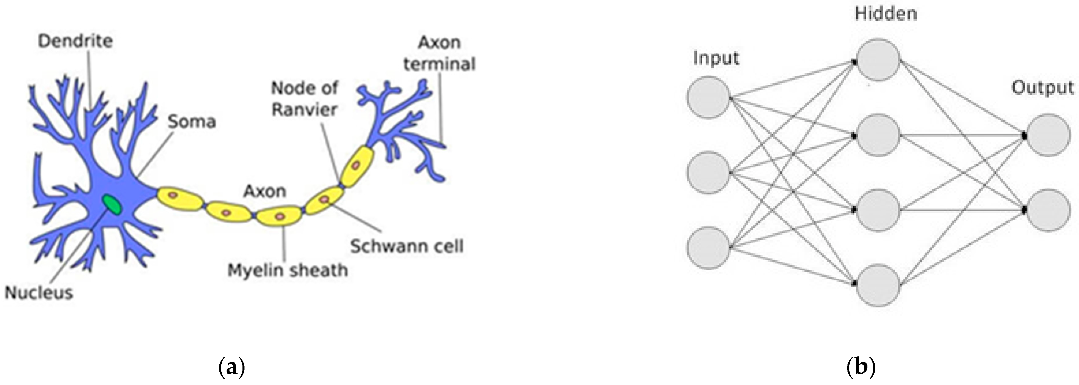
Figure 1. (a) The biological neural networks (b) The artificial neural network structure.
Computers 12 00004 g001
Figure 3. The performance results of five different algorithms based on 3-bit parity problem: (a) The curve of error function, (b) The curve of norm of gradient.
Computers 12 00004 g003aComputers 12 00004 g003b
Figure 4. The performance results of five different algorithms based on 6-bit parity problem: (a) The curve of error function, (b) The curve of norm of gradient.
Computers 12 00004 g004aComputers 12 00004 g004b
Figure 5. The performance results of five different algorithms based on function approximate problem: (a) The curve of error function, (b) The curve of norm of gradient.
Computers 12 00004 g005aComputers 12 00004 g005b
Table 1. The learning parameters for parity problems.
ProblemsNetwork StructureWeight SizeMax IterationLRRP
3-bit parity3-6-1[−0.5, 0.5]20000.0090.0003
6-bit parity6-20-1[−0.5, 0.5]30000.0060.003
Table 2. Numerical results for parity problems.
ProblemsLearning AlgorithmsAverage ErrorNorm of GradientTime (s)
3-bit parityBG L 1 / 2 3.7979 × 10−70.04221.156248
BG L 1 5.4060 × 10−77.1536 × 10−41.216248
BG L 2 9.7820 × 10−78.7826 × 10−41.164721
BGS L 1 / 2 1.7951 × 10−80.00111.155829
BGS L 1 7.6653 × 10−97.9579 × 10−51.135742
6-bit parityBG L 1 / 2 8.1281 × 10−51.166952.225856
BG L 1 3.8917 × 10−50.031652.359129
BG L 2 4.1744 × 10−50.016752.196552
BGS L 1 / 2 4.8349 × 10−50.008852.210994
BGS L 1 4.1656 × 10−60.001552.106554
Table 3. Numerical results for function approximation problem.
Learning AlgorithmsAverage ErrorNorm of GradientTime (s)
BG L 1 / 2 0.03880.35334.415500
BG L 1 0.03890.30504.368372
BG L 2 0.03900.30874.368503
BGS L 1 / 2 0.03860.29994.349813
BGS L 1 0.03790.29194.320198
Disclaimer/Publisher’s Note: The statements, opinions and data contained in all publications are solely those of the individual author(s) and contributor(s) and not of MDPI and/or the editor(s). MDPI and/or the editor(s) disclaim responsibility for any injury to people or property resulting from any ideas, methods, instructions or products referred to in the content.