Article

Latency Estimation Tool and Investigation of Neural Networks Inference on Mobile GPU

1
Skolkovo Institute of Science and Technology, 143026 Moscow, Russia
2
Faculty of Computational Mathematics and Cybernetics, Lomonosov Moscow State University, 119991 Moscow, Russia
3
Marchuk Institute of Numerical Mathematics, Russian Academy of Sciences (RAS), 119333 Moscow, Russia
4
Noah’s Ark Lab., Huawei Technologies, 121614 Moscow, Russia
*
Author to whom correspondence should be addressed.
Computers 2021, 10(8), 104; https://doi.org/10.3390/computers10080104
Submission received: 5 July 2021 / Revised: 16 August 2021 / Accepted: 18 August 2021 / Published: 23 August 2021
(This article belongs to the Special Issue Sensors and Smart Cities 2023)

Abstract

:
A lot of deep learning applications are desired to be run on mobile devices. Both accuracy and inference time are meaningful for a lot of them. While the number of FLOPs is usually used as a proxy for neural network latency, it may not be the best choice. In order to obtain a better approximation of latency, the research community uses lookup tables of all possible layers for the calculation of the inference on a mobile CPU. It requires only a small number of experiments. Unfortunately, on a mobile GPU, this method is not applicable in a straightforward way and shows low precision. In this work, we consider latency approximation on a mobile GPU as a data- and hardware-specific problem. Our main goal is to construct a convenient Latency Estimation Tool for Investigation (LETI) of neural network inference and building robust and accurate latency prediction models for each specific task. To achieve this goal, we make tools that provide a convenient way to conduct massive experiments on different target devices focusing on a mobile GPU. After evaluation of the dataset, one can train the regression model on experimental data and use it for future latency prediction and analysis. We experimentally demonstrate the applicability of such an approach on a subset of the popular NAS-Benchmark 101 dataset for two different mobile GPU.

1. Introduction

Algorithms based on convolutional neural networks can achieve high performance in numerous computer vision tasks, such as image recognition [1,2], object detection, segmentation [3], and many other areas [4]. A lot of applications require computer vision problems to be solved in real-time at the end devices, such as mobile phones, embedded devices, car computers, etc. All those devices have their architecture, hardware, and software.
Mainly, researchers optimize neural network architecture with reference to accuracy–FLOPs trade-off. However, the problem is that the real inference time of the utilized neural networks can differ significantly from theoretical, especially for mobile computing devices. For example, fast and accurate ShuffleNet [5] achieved actual speedup at Qualcomm Snapdragon 820 processor is more than 1.5 × less than theoretical in comparison with MobileNet [6]. It is a quite widespread phenomenon; more examples can be found on TensorFlow [7] Lite (TFLite) benchmark comparison [8]. More results of TensorFlow Lite performance benchmarks when running well-known models on some Android and iOS devices can be found on https://www.tensorflow.org/lite/performance/benchmarks (accessed on 19 August 2021).
The main problem is to find simultaneously fast and accurate neural network model for each target device and each target implementation. This problem is difficult and while each new device has some valuable difference in inference time for the same architecture, the task of hand-craft architecture, which optimizes the accuracy–latency trade-off directly for each new device, is too expensive and time consuming.
The promising automatic neural architecture search area (NAS) can be the solution. In this area, neural network architecture is being searched by a certain optimization algorithm maximizing combination of speed-accuracy trade-off. Already, by now, NAS methods have outperformed manually designed architectures on several tasks, such as image classification, object detection, or semantic segmentation [9]. It leads to design of the special datasets for the task of effective automatic architecture search, namely NAS-Benchmark 101 [10]/NAS-Benchmark 201 [11]. These datasets contain all possible cells generated from different number (4–7) of blocks. Each cell is represented as a directed acyclic graph. Each edge here is associated with an operation selected from a predefined operation set. We cover more detail about it in the section devoted to model parametrization. The NAS datasets contain information about training log using the same setup and the performance (on CIFAR-10/100 [12] task) for each architecture candidate, including accuracy on test set of target image classification dataset.
Many effective NAS algorithms, such as DARTS [13] and several others [14], show efficiency on those datasets but optimize architecture with respect to FLOPs number or server runtime optimization. Our scope of interest it not how architecture search algorithms actually perform, but what proxy is used as architecture complexity/inference time. As soon as actual speed on target device is much more valuable for applications than complexity in number of operations. In work on MnasNET [11], authors applied NAS for architecture search and provided measurements for each proposed model on a mobile CPU. Thus, they proposed a very efficient architecture for mobile device utilization, but without the use of the mobile GPU. They implemented models in TensorFlow Lite and directly measured real-world inference time by executing the model on mobile phones for performing NAS. Of course, this approach requires making a lot of real-world experiments on target device.
In EfficientNet-EdgeTPU [15], researchers use the other solution. They implemented a precise simulator of the target device (mobile CPU), which can run in parallel on regular clusters, but that way is a quite complex engineering task. It is also implemented with TFLite. Cheaper and lighter approach is used by authors of ProxylessNAS [16], ChamNet [17], and FBNet [18]. Models in these works were deployed with Caffe2 with highly efficient int8 implementation. Authors created a lookup table (LUT) of all blocks. After that, latency is computed as a sum of latencies of the corresponding blocks. This approach is quite efficient for mobile CPU latency modeling and does not require massive experiments on target devices.
Surprisingly, while GPU or special NPU (neural processing units) are preferable for neural network inference, there are only a few works about latency modeling for mobile GPU for now. In work on MOGA [19], GPU-awareness was investigated for the different search space, and authors state that the aforementioned lookup table works well even for mobile GPU, but for cases when latency is calculated for each block of the same structure and input shape. The models were deployed in TensorFlow Lite in that work. In contrast, authors on BRP-NAS [20] considered a lookup table approach as inefficient for GPU latency prediction and proposed their own method based on graph convolution network (GCN) but did not provide any source code or open dataset. They implemented experiments on a mobile device with not so the widespread Snapdragon Neural Processing Engine framework (SNPE). In our setup, we obtain that LUT gives quite high error for layer-wise prediction of neural network latency on a mobile GPU.
To the best of our knowledge, the latency modeling area is in its early stage of development currently, and there are no common ways to find a good approximation of neural network inference time/speed, especially on mobile GPU. This research is aimed to find the way to fill this gap with the proposed approach and LETI pipeline. Latency is also very dependent on the CPU or GPU architecture, a number of cores, processing units, memory hierarchy, bandwidth between memory levels, etc. In addition, it is very important to optimize the software implementation to the target architecture (how to layout data and perform processing of them). We hope to address these issues in our future research.
It is worth it to mention an important detail: in addition to dependence on hardware, the inference time of neural networks also highly depends on implementation [21]. In this work, we study inference of TensorFlow Lite models on a mobile GPU and propose an Latency Estimation Tool (LETI) for reconstructing models from graph-based parametrization; estimation and modelling latency. Our tool is implemented as two Python packages. Neural networks are implemented as TensorFlow 2 Keras (TF.Keras) models. The tool provides a convenient way to convert them into the TensorFlow Lite model with a standard TensorFlow Converter. We assume that our tool is potentially useful for NAS research because it can create all possible models from the desired parametrization and evaluate their TFLite versions on the target device’s CPU/GPU or NPU. To set up the desired search space, the researcher has to define parametrization. We use it the same as in the NAS-Benchmark-101 in our experiments.
Our main contributions are:
  • LETI Tool, which allows:
    -
    To generate TF.Keras models from parametrization, with parametrization same as in NAS-Benchmark-101.
    -
    To evaluate TF.Keras model on CUDA devices.
    -
    To convert to TFLite using TF converter and evaluate on Android device.
    -
    To encapsulate latency evaluation on device as black-box for direct optimization (e.g., with Nevergrad [22]).
  • Evaluation of lookup table for several popular neural networks on a mobile CPU and providing an tool for such estimation.
  • Evaluation of latency prediction methods on generated latency dataset: RANSAC [23] regression on FLOPs number with and without clustering based on peak memory usage; XGBoost [24]; CatBoost [25]; LightGBM [26]; and graph convolution network (GCN) for latency prediction on a mobile GPU.

2. Materials and Methods

2.1. Neural Network Parametrization

The parametrization of neural networks is crucial for defining architectures. In our work, we exploit the approach from NAS-Bench-101 [10]. We represent a neural network as a directed graph with nodes representing layers and edges representing connections (see Figure 1). We store correspondence between the number of nodes and layers in a special list (layers_list).
A graph can be represented with the adjacency matrix. For a simple graph with the vertex set V, the adjacency matrix is a square | V | × | V | matrix A such that its element A i j is one when there is an edge from vertex i to vertex j, and zero when there is no edge.
One needs to specify the adjacency matrix, the list of layers, and the configuration dictionary to set up the complete implementation of the desired neural network. Our tool can be used to generate the selected list of desired models or for the whole dataset generation. The entire process from settings to evaluation requires several steps, which we describe in the next subsection.

2.2. Latency Dataset Generation Pipeline

Below, we describe the pipeline of the generation of the latency dataset. The scheme of the pipeline can be found in Figure 2 and has the following form:
  • Firstly, we generate the set of parametrized architectures as in NAS-Benchmark. We verify uniqueness by the same hashing procedure as in Reference [10]. Thus, it is additional proof of the same parametrization and set of models. For NAS-Benchmark configuration at this step, we obtain 423,624 parametrized models/graphs with: max 7 vertices, max 9 edges with 3 possible layer values (except input and output): [‘conv3x3-bn-relu’, ‘conv1x1-bn-relu’, ‘maxpool3x3’].
  • Next, we generate TF.Keras models. The tool is able to generate both only the basic block that is represented by the parametrization or the stacked models built from such blocks as in the NAS-Bench-101.
  • Then, we build models for the specified input shape and convert it into TensorFlow Lite representation.
  • After, we optionally evaluate the latency of TF.keras models on desktop/server GPU nodes. In our work, we run the model for n 100 times with guaranteed condition on standard deviation: s t d ( r u n s _ l a t e n c y ) 1 10 m e a n ( r u n s _ l a t e n c y ) .
  • Finally, we evaluate the latency of TFLite models on the CPU, GPU, or NPU of the Android devices. In work, we evaluate only models which are fully delegated to GPU for TFLite Some operations are not supported for delegation by the framework, such as SLICE. See operations descriptions at: https://www.tensorflow.org/lite/guide/ops_compatibility (accessed on 19 August 2021). Part of the models use the addition of more than two intermediate layers, that ADD_N operation in TFLite, that is also unsupported by GPU. We substitute that operation with multiply ADD operation (addition of two tensors can be delegated for mobile GPU).
Figure 2. Latency dataset generation pipeline.
Computers 10 00104 g002
The dataset stores the sequence of tested architectures. Each item in this sequence is represented with its unique hash code, list of layers, their adjacency matrix, and timings of measurements (in milliseconds) for evaluated devices. We also supported these items with estimates of their execution cost in FLOPs and measured Peak memory consumption that is useful for some modeling methods.

3. Results

In this section, we show the construction and analysis of the dataset we constructed for two mobile devices and the subset of NAS-Bench 101 search space.
The goal of our work is to build a convenient way to collect data and create a hardware-specific latency predictor. In this work, we focus on a mobile GPU. For testing our framework, we chose two mobile devices based on Huawei Kirin 970 (GPU: ARM Mali-G72 MP12) and Kirin 980 (GPU: ARM Mali-G76 MP10).

3.1. Discussion about Choosing Implementation and Deploying on Mobile Devices

In this subsection, we discuss deployment on mobile devices because this work is mostly targeted on it. Currently, there are two most popular operating systems for smartphones: iOS and Android. Android maintains its position as the leading mobile operating system worldwide, controlling the mobile OS market with a close to 73 percent share. This is the reason to focus firstly on Android devices.
There are several ways to run artificial neural network on Android-based devices. The most common way is to use special deep learning framework. Currently, most of applications use TensorFlow Lite, Caffe2 [27], or very fresh Pytorch Mobile [28] (experimental in the end of 2019, released in 2020, NNAPI added in the end of 2020). Different implementations of the very same neural network architecture can vary in performance, weight, and inference time even on the same hardware [29]. First of all, model can be run on a CPU, GPU, or special NPU of a device if the implementation allows it to be done. Furthermore, the same implementation of the neural network can significantly differ device-to-device (see figures from Reference [29] for bright examples). In addition, some frameworks propose quantizing operation which provides a significant speed-up of the inference. Often, this is the reason to choose TensorFlow Lite, because this operation was added to Pytorch Mobile only recently, a couple of years later than in TensorFlow Lite. We choose TensorFlow lite due to its popularity and relative stability. We do not use quantization or pruning in our experiments, but, with same pipeline, it is possible to add it as a parameter in architecture representation. We do not focus on delegation on NPU, but it is a result.
Our target is create a new way to search neural network in both implementation and hardware-specific way. We do not aim to achieve top accuracy but, rather, to show that, even using simple baseline machine learning methods, it is possible to choose neural network more accurately than just based on number of operations (FLOPs). We create our experiments with full delegation on a mobile GPU using TensorFlow Lite framework for two Kirin devices. The choice of device highly depends on the application. For example, for a standard CV application inside pre-installed Camera app on Huawei, it is natural to use Huawei devices. For developing general-purpose application it is better to separate it into several main architectures and choose specific implementation and architecture for each one. Therefore, without covering too wide-spread set of devices (including Arm Cortex CPUs/Mali GPU, Google Pixel chipsets, Samsung chipsets, MediaTek chipsets, HiSilicon chipsets, Qualcomm chipsets, etc.; see Reference [21]), any choice may not be sufficient for all tasks. However, creating datasets for all possible architectures seems to be redundant for demonstration of our pipeline and methodology. We choose Huawei Kirin devices with different CPU and GPU based on Kirin 970 and Kirin 980 SoCs. For CPU lookup experiments, we also use device of another manufacturer, i.e., a Samsung Exynos 9810 device, that was in stock. We present information about the devices in Table 1.
Cache sizes (L1/L2/L3, if it has) for used cores are: Exynos 9810-Exynos M3 (384KiB/2MiB/4MiB), Cortex-A55 (256KiB/256KiB); Kirin 970-Cortex-A73 (512KiB/2MiB), Cortex-A53 (256KiB/1MiB); Kirin 980-Cortex-A76 (512KiB/2MiB), Cortex-A55 (256KiB/512KiB). For CPU experiments, we run the task on a BIG core in 1 thread.

3.2. TensorFlow Lite Dataset

For evaluation on a mobile GPU, we create a dataset consisting of 11,055 samples for fully GPU delegable 96 × 96 × 3 cells. We split it into the training dataset (1000 samples) and the testing dataset (10,055 samples). Nine thousand eight hundred and ninety-four out of 110,55 samples represent delegable accurate and fast models: for each of that number operations, less than 5 × 10 9 FLOPs and full stacked model have accuracy more than 93.21% on CIFAR-10 based on NAS-Benchmark 101 data (see Figure 3). The rest models are randomly subsampled architectures. We subsampled a lot of models, but a minority of randomly sampled models were evaluated on GPU successfully, which move us to focus on a limited subsample from the original search space.
We train and evaluate models using cross-validation with splitting train dataset (totally only 1000 samples) into folds. After the model is selected, it trains on the whole training dataset, and, after that, models were not changed. The final evaluation is conducted on the test dataset (10,055 samples).
Each experiment, if not mentioned otherwise, contains 300 runs and is restarted if the standard deviation of the latency is more than 10% of the mean. In addition, we collect the dataset 3 times and correlate results from different experiments (see results for Kirin 970 in Figure 4a,b). We delete all results that differ more than 10%. It is noticeable that, in very rare cases, there is a huge difference in measurements. We do not investigate that issues, but our guess is that they can be connected with some non-optimized benchmark and framework implementation issues.
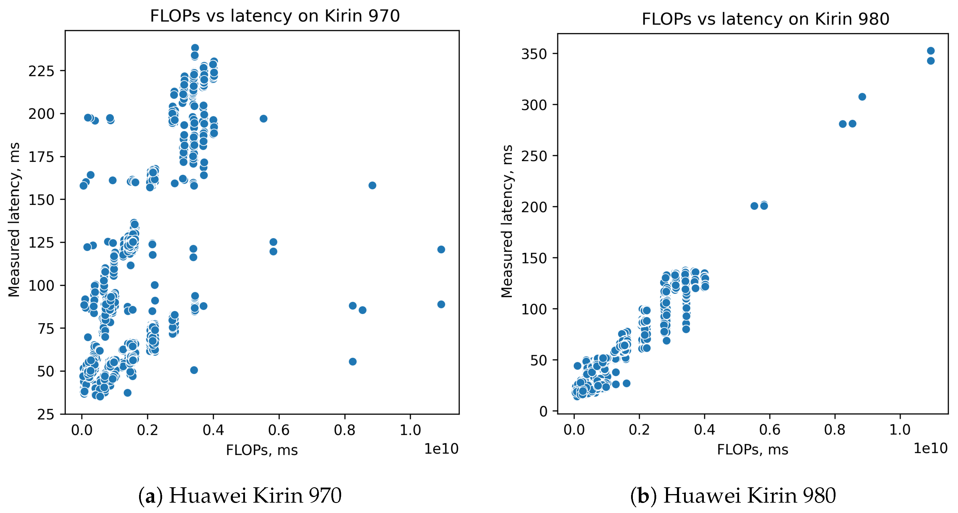
We investigated the dependency from the number of operations for both collected datasets (see Figure 5a,b). One can see that, for Kirin 970, dependence from FLOPs is not so linear as for Kirin 980. This non-linear behavior can be connected with different GPU cache size (1MB for Kirin 970 (Mali-G72 MP12), 2MB for Kirin 980 (Mali-G76 MP10)). According to Figure 6b, we can see that heavy models are generally slow, while the majority of the light ones are fast. In addition, we suppose that, while TensorFlow Lite is not hardware-specific, it can work more optimally on Mali-G76 than Mali-G72. We consider that such investigation can be highly useful for developers and leave it for further research.

4. Latency Modeling

Since our goal is to create a tool for the generation of the latency dataset, we also evaluate some models to show how LETI can be used for creating latency proxy.

4.1. Lookup Table on Mobile CPU and GPU

In this section, we discuss the results of the application of the lookup table (LUT) method to latency prediction. Before creating our tool, based on current best practices, we evaluate several popular architectures in TFLite to test this approach on real mobile devices. We use Huawei Kirin 970 (GPU Mali-G72 MP12), Huawei Kirin 980 (Mali-G76 MP10), and Samsung Exynos 9810 (Mali-G72 MP18).
We implement the lookup table method, which is used in ProxylessNAS, ChamNet, FBNet for the prediction of latency on a mobile CPU. Firstly, we implemented an automatic tool that decomposes the TF.Keras model into a sequence of blocks. We use a single layer as a block. After that, we initialize inputs for each block with the correct input tensor (for the first one, it is image shape: 224 × 224 × 3; for the second one, it is the shape of the first block’s output). After that, we convert these blocks as standalone TFLite models and deploy them on the device for evaluation. We evaluate each block’s inference time within 300 runs and put the value into the lookup table. After that, we fill all the required layers and compute total latency as the sum of corresponding blocks. The speed of a single layer is measured directly with TensorFlow-Benchmark.
From Table 2, we see that the approach based on the exploitation of the lookup table works quite well for the prediction of the inference times for the popular models at CPUs of different mobile devices.
We use the same method and create the lookup table for GPU delegation, but it results in extremely low precision. We suppose that, due to the huge impact of additional operations and a possibly different approach to work with RAM, it seems impossible to directly apply the lookup table method for satisfactory latency predictions at a GPU or NPU.
Hence, we assume that it would be better to try more general machine learning approaches and firstly create the tool for the generation dataset of models, their implementations, and experimentally measured latencies on different devices.

4.2. Linear Models Based on FLOPs

The baseline is just to use FLOPs as a latency proxy. There are several ways how to fit it, for example, optimize least square error (linear regression). We choose a more robust version based on the random samples consensus (RANSAC) method because data contains a lot of outliers. The scatter plots of fitted model are in Figure 7a,b. Results will be presented in Table 3 at the end of the section.
While a linear model based on FLOPs is good enough for Kirin 980 dataset, it is not for Kirin 970. In addition, that fact illustrates that latency prediction on a mobile GPU is a very case-specific problem. Analyzing data for Kirin 970, we found that there are two domains and would like to fit a linear model for each one. We assumed that domains are connected with memory consumption and measured peak memory for all models in the dataset (Figure 6b). We chose to separate domains based on memory thresholding. The threshold is adjusted automatically by optimizing the sum of variances of latencies in domains for the training subset (folds from 100 samples). We named models constructed using that way “RANSAC + cluster”, and they are a better fit for the data (see Figure 6a and Table 3).

4.3. Gradient Boosting Methods

Obviously, one can use not only FLOPs as input data for predictions. We concatenate FLOPs, peak memory, flatten adjustment matrix, and layers list as input vector size 2 + 7 2 + 7 = 58 . Latency is used as the target. Such a dataset allows easily testing of a lot of regression models. Here, we provide a regression model based on different gradient boosting methods: XGBoost, CatBoost, and LightGBM.
A gradient boosting procedure [30] builds iteratively a sequence of approximation functions F t : R m R , t = 0 , 1 , in a greedy fashion. Namely, F t is obtained from the previous approximation F t 1 in an additive manner: F t = F t 1 + α h t , where α is a step size, and function h t : R m R (a base predictor) is chosen from a family of functions H, in order to minimize the expected loss L ( y t r u e , y p r e d ) :
h t = argmin h H L ( F t 1 + h ) = argmin h H E L ( y , F t 1 ( x ) + h ( x ) ) .
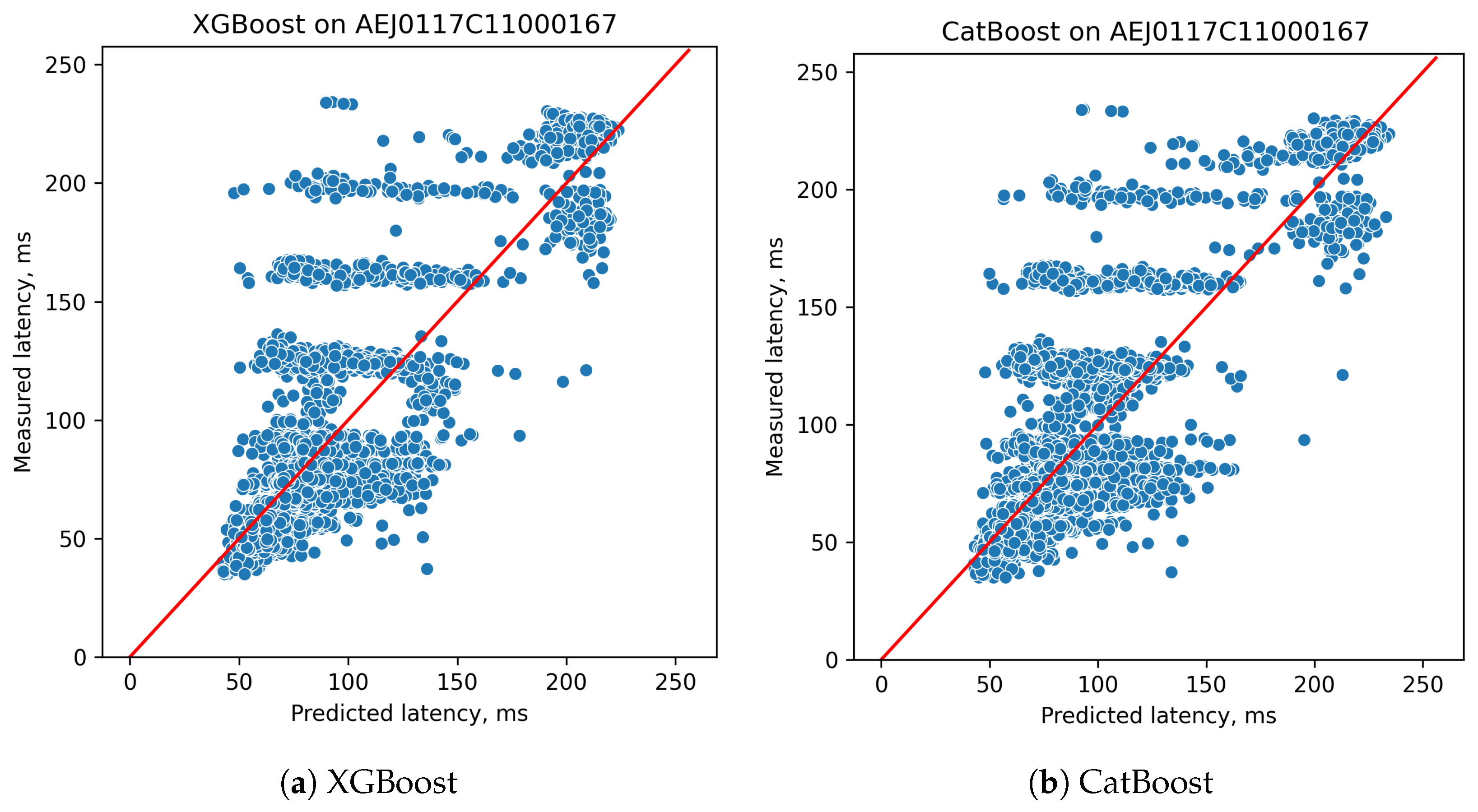
More detailed discription of methods are in original papers: XGBoost [24]; CatBoost [25]; LightGBM [26]. In Figure 8a,b and Figure 9a, the scatter plots of predicted inference time to measured one are presented. There are minor difference in the results, as shown in Table 3.

4.4. Graph Convolutional Network (GCN) for Latency Prediction

In a paper on BRP-NAS [20], authors use GCNs for latency prediction on desktop CPU/GPU and embedded (Jetson Nano) GPU and achieve good results for networks from NAS-Bench 201 dataset.
GCN latency predictor consists of a graph convolutional network which learns models for graph-structured data [31]. Given a graph g = ( V , E ) , where V is a set of N nodes with D features, and E is a set of edges, a GCN takes as input a feature description X R N × D and a description of the graph structure as an adjacency matrix A R N × N . For an L-layer GCN, the layer-wise propagation rule is the following:
H l + 1 = f ( H l , A ) = σ A H l W l ,
where H l and W l are the feature map and weight matrix at the l-th layer, respectively, and σ ( ) is a non-linear activation function, such as ReLU. H 0 = X and H L is the output with node-level representations. See the illustration in Figure 9b.
We use 4 layers of GCNs, with 600 hidden units in each layer. After that, we use a fully connected (dense) layer with ReLU activation that generates one scalar prediction—inference time. The input of GCN is encoded by an adjacency matrix A and a feature matrix X (one-hot encoding of layer/block type). The scatter plot of predicted latency to measured is presented in Figure 10.

4.5. Numerical Results for Proposed Methods

Using the LETI tool, we collect two datasets and show how different methods can be applied for each one. We tried six methods and measured them. For the numerical results, we use two metrics: the percentage of models with predicted latency within the corresponding error bound relative to the measured latency (Acc@10% for ± 10 % bound) and coefficient of determination R 2 .
If dataset has n values marked y 1 , , y n , each is associated with a predicted value f 1 , , f n . If y ¯ is the mean of the observed data: y ¯ = 1 n i = 1 n y i , then the variability of the dataset can be measured with two sums of squares formulas: The total sum of squares (proportional to the variance of the data):
S S tot = i ( y i y ¯ ) 2 .
The sum of squares of residuals, also called the residual sum of squares, is:
S S res = i ( y i f i ) 2 .
The most general definition of the coefficient of determination is:
R 2 = 1 S S res S S tot .

5. Discussion

In this section, we discuss ways how the obtained methodology can be perceived in perspective of previous studies. Currently, there are only a few ways to approximate inference time on mobile devices. All of them have their own pro and contra. Mainly, they are:
  • FLOPs
    Advantages: Easy to calculate. Gives information about number of computational operations, and it is obviously connected with latency.
    Disadvantages: Different operations can require different times to perform. In addition, that is both implementation and hardware-specific. Several devices, such as GPU, have very nonlinear dependency of inference time from number of operations. Data movement operations is not taken into account at all because, formally, it is not a computational operation, but it takes some time, and, sometimes, it may be significant.
  • Lookup Table
    Advantages: Requires only small number of experiments as large as number of all possible blocks.
    Disadvantages: It does not count data movement between blocks, model loading on device, which can take a lot of inference.
  • Build Simulator of target device
    Advantages: Allows getting precise estimation of inference time without real experiments. More robust, than experiments on a mobile device. Can be run in parallel on clusters.
    Disadvantages: Requires complex engineering work to construct simulator of each target hardware. Seems to be hard to use for not-CPU devices.
  • Direct measurements on device for each model
    Advantages: Allows getting real estimation of inference time, the direct method. It has the best match to real user experience.
    Disadvantages: Inference time can highly vary from run to run and needs a series of experiments to get robust estimation. A huge number of experiments is required and leads to either long experiments or requires a huge cluster of same devices to conduct parallel experiments.
  • Direct measurements for small subset of models and construction of prediction model
    Advantages: Requires tracktable in time number of real-world experiments for even one test device. Gets real experimental values for latency corresponding to user experience.
    Disadvantages: Model can be not as precise as direct measurements. Training subset of neural network search space can be not representative enough to cover the whole search space.
In our work, we provide the pipeline for the last approach. We can find the only example of usage of such methodology in BRP-NAS [20], where researchers succeeded in training graph convolutional network to predict latency of neural network. In our project, we do not succeed with the same approach, probably due not proper architecture or training. However, the other baselines work with reasonable precision, especially if one takes into account that even direct measurements of provided models often require more than 300 runs to get a standard deviation of inference time less than 10% from the mean value. So, even the “approximate” values of latency is useful.

6. Conclusions

This work presents a novel tool and discusses its exploitation for the generation and investigation of neural networks with user-defined parametrization.
Latency prediction on a mobile GPU that currently a barely researched area, but it is a very important one. We hope that the deep learning community will give more attention to that because real applications tend to be run on mobile devices, and hardware-specific solutions are highly needed. From our perspective, the LETI approach has a high potential for that task.
We show an example of applying the developed toolbox to automatic latency prediction problems for generation latency datasets for desktop and Android devices. The collected dataset allows us to demonstrate non-trivial relations from peak memory size, floating operations, and neural networks’ inference times for a mobile GPU, which are also barely investigated, despite having a huge impact on real-life applications based on neural networks.
While focusing on a mobile GPU, we test several latency prediction baselines. We consider that a lookup table works well for the CPU-based devices approach for prediction of latency of neural networks but is not accurate on GPU. More general machine learning regression models or GCN can be good solutions in particular cases and can be easily constructed after collecting a small subset from the generated dataset. We hope that this study can be highly useful for developers who want to run real-time computer vision applications on mobile devices and accelerate research in latency modeling.

Author Contributions

Conceptualization, I.O. and V.G.; methodology, E.P., I.O. and S.M.; software, E.P.; validation, E.P. and V.G.; formal analysis, E.P.; investigation, E.P.; resources, V.G.; data curation, E.P.; writing—original draft preparation, E.P.; writing—review and editing, S.M.; visualization, E.P.; supervision, I.O., V.G.; project administration, S.M.; funding acquisition, V.G. All authors have read and agreed to the published version of the manuscript.

Funding

The reported study was funded by RFBR, project No.19-29-09085 and No.19-31-90172.

Institutional Review Board Statement

Not applicable.

Informed Consent Statement

Not applicable.

Data Availability Statement

The data and code are private, can be available upon request.

Acknowledgments

We thank the editor and three anonymous reviewers for their constructive comments, which helped us to improve the manuscript.

Conflicts of Interest

The authors declare no conflict of interest.

Abbreviations

The following abbreviations are used in this manuscript:
LETILatency estimation tool and investigation of neural networks inference
FLOPFloating point operations
GPUGraphics processing unit
CPUCentral processing unit
NPUNeural processing unit
RFBRRussian Foundation for Basic Research
NASNeural architecture search
LUTLookup table
TFLiteTensorFlow Lite
TF.KerasTensorFlow Keras

References

  1. Krizhevsky, A. ImageNet classification with deep convolutional neural networks. Commun. ACM 2017, 60, 84–90. [Google Scholar] [CrossRef]
  2. He, K. Identity mappings in deep residual networks. Lect. Notes Comput. Sci. 2016, 9908, 630–645. [Google Scholar]
  3. Lin, T. Microsoft COCO: Common objects in context. Lect. Notes Comput. Sci. 2014, 8693, 740–755. [Google Scholar]
  4. Wani, M. Advances in Deep Learning; Springer: Singapore, 2020. [Google Scholar]
  5. Zhang, X.; Zhou, X.; Lin, M.; Sun, J. ShuffleNet: An Extremely Efficient Convolutional Neural Network for Mobile Devices. In Proceedings of the IEEE Computer Society Conference on Computer Vision and Pattern Recognition, Salt Lake, UT, USA, 18–23 June 2018. [Google Scholar]
  6. Howard, A.G.; Zhu, M.; Chen, B.; Kalenichenko, D.; Wang, W.; Weyand, T.; Andreetto, M.; Adam, H. Mobilenets: Efficient convolutional neural networks for mobile vision applications. arXiv 2017, arXiv:1704.04861. [Google Scholar]
  7. Abadi, M.; Barham, P.; Chen, J.; Chen, Z.; Davis, A.; Dean, J.; Devin, M.; Ghemawat, S.; Irving, G.; Isard, M.; et al. TensorFlow: A system for large-scale machine learning. In Proceedings of the 12th USENIX Symposium on Operating Systems Design and Implementation, OSDI, Savannah, GA, USA, 2–4 November 2016. [Google Scholar]
  8. Lee, J.; Chirkov, N.; Ignasheva, E.; Pisarchyk, Y.; Shieh, M.; Riccardi, F.; Sarokin, R.; Kulik, A.; Grundmann, M. On-device neural net inference with mobile gpus. arXiv 2019, arXiv:1907.01989. [Google Scholar]
  9. Zoph, B.; Vasudevan, V.; Shlens, J.; Le, Q.V. Learning Transferable Architectures for Scalable Image Recognition. In Proceedings of the IEEE Computer Society Conference on Computer Vision and Pattern Recognition, Salt Lake, UT, USA, 18–23 June 2018. [Google Scholar]
  10. Ying, C.; Klein, A.; Christiansen, E.; Real, E.; Murphy, K.; Hutter, F. NAS-bench-101: Towards reproducible neural architecture search. In Proceedings of the 36th International Conference on Machine Learning, Long Beach, CA, USA, 9–15 June 2019; pp. 7105–7114. [Google Scholar]
  11. Dong, X.; Yang, Y. Nas-bench-201: Extending the scope of reproducible neural architecture search. In Proceedings of the International Conference on Learning Representations, Online, 26 April–1 May 2020. [Google Scholar]
  12. Krizhevsky, A.; Nair, V.; Hinton, G. Learning Multiple Layers of Features from Tiny Images. Available online: https://www.cs.toronto.edu/~kriz/learning-features-2009-TR.pdf (accessed on 19 August 2021).
  13. Liu, H.; Simonyan, K.; Yang, Y. DARTS: Differentiable architecture search. In Proceedings of the International Conference on Learning Representations, New Orleans, LO, USA, 6–9 May 2019. [Google Scholar]
  14. He, X.; Zhao, K.; Chu, X. AutoML: A Survey of the State-of-the-Art. In Knowledge-Based Systems; Elsevier: Amsterdam, The Netherlands, 2021. [Google Scholar]
  15. Google AI Blog: EfficientNet-EdgeTPU: Creating Accelerator-Optimized Neural Networks with AutoML. Available online: https://ai.googleblog.com/2019/08/efficientnet-edgetpu-creating.html (accessed on 19 August 2021).
  16. Cai, H.; Zhu, L.; Han, S. ProxylessNAS: Direct neural architecture search on target task and hardware. In Proceedings of the International Conference on Learning Representations, New Orleans, LO, USA, 6–9 May 2019. [Google Scholar]
  17. Dai, X.; Zhang, P.; Wu, B.; Yin, H.; Sun, F.; Wang, Y.; Dukhan, M.; Hu, Y.; Wu, Y.; Jia, Y.; et al. Chamnet: Towards efficient network design through platform-aware model adaptation. In Proceedings of the IEEE Conference on Computer Vision and Pattern Recognition, Long Beach, CA, USA, 16–20 June 2019; pp. 11398–11407. [Google Scholar]
  18. Wu, B.; Dai, X.; Zhang, P.; Wang, Y.; Sun, F.; Wu, Y.; Tian, Y.; Vajda, P.; Jia, Y.; Keutzer, K. FBnet: Hardware-aware efficient convnet design via differentiable neural architecture search. In Proceedings of the IEEE Conference on Computer Vision and Pattern Recognition, Long Beach, CA, USA, 16–20 June 2019; pp. 10734–10742. [Google Scholar]
  19. Chu, X.; Zhang, B.; Xu, R. MOGA: Searching beyond mobilenet v3. In Proceedings of the International Conference on Acoustics, Speech, and Signal Processing, Barcelona, Spain, 4–8 May 2020. [Google Scholar]
  20. Dudziak, Ł.; Chau, T.; Abdelfattah, M.S.; Lee, R.; Kim, H.; Lane, N.D. BRP-NAS: Prediction-based NAS using GCNs. In Proceedings of the Conference on Neural Information Processing Systems, Online, 6–12 December 2020. [Google Scholar]
  21. Ignatov, A.; Timofte, R.; Chou, W.; Wang, K.; Wu, M.; Hartley, T.; Van Gool, L. AI Benchmark: Running deep neural networks on android smartphones. Lect. Notes Comput. Sci. 2019. [Google Scholar] [CrossRef] [Green Version]
  22. Rapin, J.; Teytaud, O. Nevergrad—A Gradient-Free Optimization Platform. 2018. Available online: https://github.com/facebookresearch/nevergrad (accessed on 19 August 2021).
  23. Martin, A. Fischler and Robert C. Bolles. Random sample consensus: A paradigm for model fitting with applications to image analysis and automated cartography. Commun. ACM 1981, 24, 381–395. [Google Scholar]
  24. Chen, T.; Guestrin, C. XGBoost: A scalable tree boosting system. In Proceedings of the ACM SIGKDD International Conference on Knowledge Discovery and Data Mining, New York, NY, USA, 13–17 August 2016; pp. 785–794. [Google Scholar]
  25. Prokhorenkova, L.; Gusev, G.; Vorobev, A.; Dorogush, A.V.; Gulin, A. CatBoost: Unbiased boosting with categorical features. arXiv 2017, arXiv:1706.09516. [Google Scholar]
  26. Ke, G.; Meng, Q.; Finley, T.; Wang, T.; Chen, W.; Ma, W.; Ye, Q.; Liu, T.-Y. LightGBM: A Highly Efficient Gradient Boosting Decision Tree. Technical Report. 2017. Available online: https://dl.acm.org/doi/pdf/10.5555/3294996.3295074 (accessed on 19 August 2021).
  27. Caffe2. Available online: https://caffe2.ai/ (accessed on 19 August 2021).
  28. Pytorch Mobile. Available online: https://pytorch.org/mobile/home/ (accessed on 19 August 2021).
  29. Luo, C.; He, X.; Zhan, J.; Wang, L.; Gao, W.; Dai, J. Comparison and Benchmarking of AI Models and Frameworks on Mobile Devices. arXiv 2020, arXiv:2005.05085v1. [Google Scholar]
  30. Friedman, J.H. Greedy function approximation: A gradient boosting machine. Ann. Stat. 2001, 29, 1189–1232. [Google Scholar] [CrossRef]
  31. Kipf, T.N.; Welling, M. Semi-Supervised Classification with Graph Convolutional Networks. In Proceedings of the International Conference on Learning Representations, Toulon, France, 24–26 April 2017. [Google Scholar]
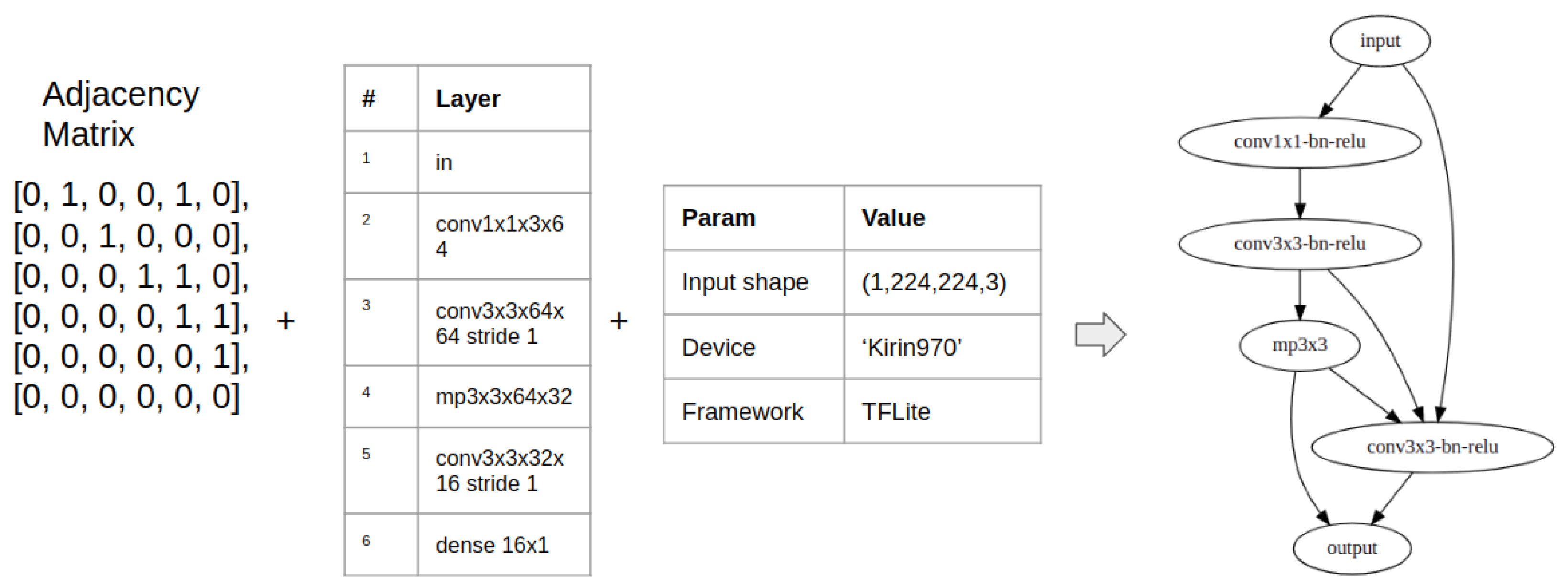
Figure 1. Parametrization of neural network implementation as a set of adjacency matrix, layers list, and config dict.
Computers 10 00104 g001
Figure 3. Dependency between latency and accuracy on CIFAR-10 of network with same base cell | Huawei Kirin 970.
Computers 10 00104 g003
Figure 4. Estimated latency for (a) runs #1 and #2; (b) runs #2 and #3. Both are on a Huawei Kirin 970 device.
Computers 10 00104 g004
Figure 5. Dependency between latency and number of FLOPs for (a) Huawei Kirin 970, (b) Huawei Kirin 980 devices.
Computers 10 00104 g005
Figure 6. Dependency between predicted latency by two RANSAC models based on memory clusters and measured (a) and dependency between measured latency and peak memory usage (b). Both are for a Huawei Kirin 970 device.
Computers 10 00104 g006
Figure 7. Dependency between latency predicted by RANSAC versus measured on test subset for (a) Huawei Kirin 970, (b) Huawei Kirin 980 devices.
Computers 10 00104 g007
Figure 8. Dependency between latency predicted by (a) XGBoost or (b) CatBoost and measured on test subset on a Huawei Kirin 970 device.
Computers 10 00104 g008
Figure 9. Dependency between latency predicted by (a) LightGBM or (b) GCN and measured on test subset on a Huawei Kirin 970 device.
Computers 10 00104 g009
Figure 10. Graph Convolutional Network (GCN) for latency prediction.
Computers 10 00104 g010
Table 1. Details about the devices which we utilized in our research.
Device NameKirin 970Kirin 980Exynos 9810
Serial numAEJ0117C11000167015NTV187K000112R39K708F15
Lithography10 nm7 nm10 nm
Release date02/09/201731/08/201701/03/2018
ArchitectureARM big.LITTLEARM big.LITTLEARM big.LITTLE
SeriesCortex-A73/-A53Cortex-A76/-A55Exynos M3/Cortex-A55
4x Cortex-A73 (2.4 GHz) +2x Cortex-A76 (2.6 GHz) +4x Exynos M3 (2.9 GHz) +
CPU4x Cortex-A53 (1.8 GHz)2x Cortex-A76 (1.9 GHz) +4x Cortex-A55 (1.9 GHz)
4x Cortex-A53 (1.8 GHz)
MemoryLPDDR4XLPDDR4XLPDDR4X
GPUARM Mali-G72 MP12ARM Mali-G76 MP10ARM Mali-G72 MP18
GPU Lith.16 nm7 nm16 nm
GPU clock746 MHz720 MHz572 MHz
GPU Execut.12 units10 units18 units
GPU Shading192 units160 units288 units
GPU Cache1 MB2 MB1 MB
GPU Perf286 GFLOPS (FP32)230 GFLOPS (FP32)370 GFLOPS (FP32)
Table 2. Latency, measured by direct method and as a sum of block’s latencies for mobile CPU. The lookup table method allows for obtaining good accuracy of predictions.
ModelResnet50Resnet50NASNet
DeviceKirin 980Exynos 9810Exynos 9810
Direct, ms552 ± 7.11806 ± 20.2432 ± 3.1
LUT, ms620 ± 3.61714 ± 53.0388 ± 7.3
Error, ms68.192.243.8
Rel. err.12.32%5.38%11.29%
Table 3. Accuracy for tolerance threshold 10% (metric same as in BRP-NAS [20]) and R 2 . Results for all discussed methods on two collected datasets (on Kirin 970 and 980) with train/test splitting 1000/10,055 samples. Bold texts indicate the best results.
Acc@10% R 2
Method/Device970980970980
RANSAC68.2980.140.040.93
RANSAC + cluster71.3184.110.510.93
LightGBM49.1784.790.740.90
XGBoost57.5185.580.770.92
CatBoost55.5586.100.7650.93
GCN44.6167.160.690.81
Publisher’s Note: MDPI stays neutral with regard to jurisdictional claims in published maps and institutional affiliations.