
Prediction of Rapid Early Progression and Survival Risk with Pre-Radiation MRI in WHO Grade 4 Glioma Patients

 ,
,  and
and
Abstract
:Simple Summary
Abstract
1. Introduction
2. Materials and Methods
2.1. Patient Data
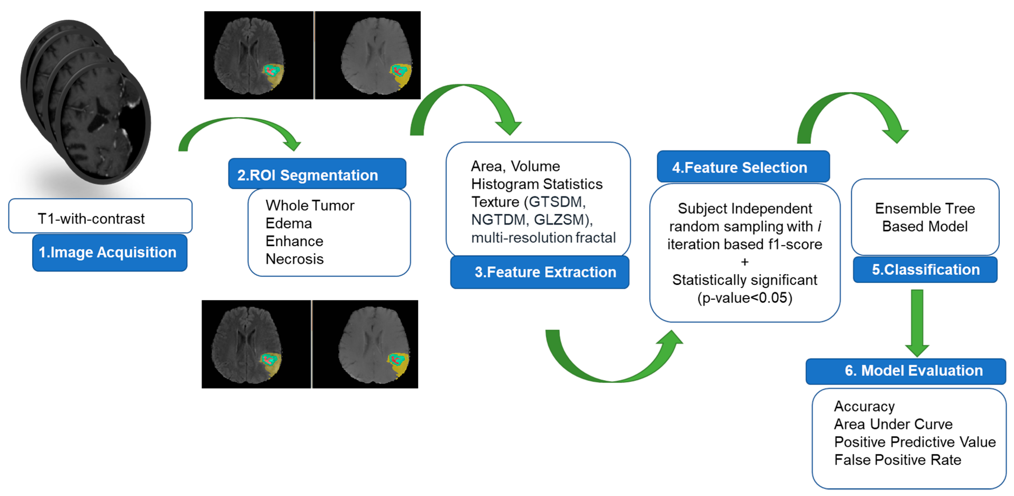
2.2. Algorithm Pipeline for Prediction of Rapid Early Progression (REP)
2.3. MRI Preprocessing, Tumor Volume Segmentation and Feature Extraction
2.3.1. MRI Preprocessing
2.3.2. Tumor Volume Segmentation
2.3.3. Feature Extraction
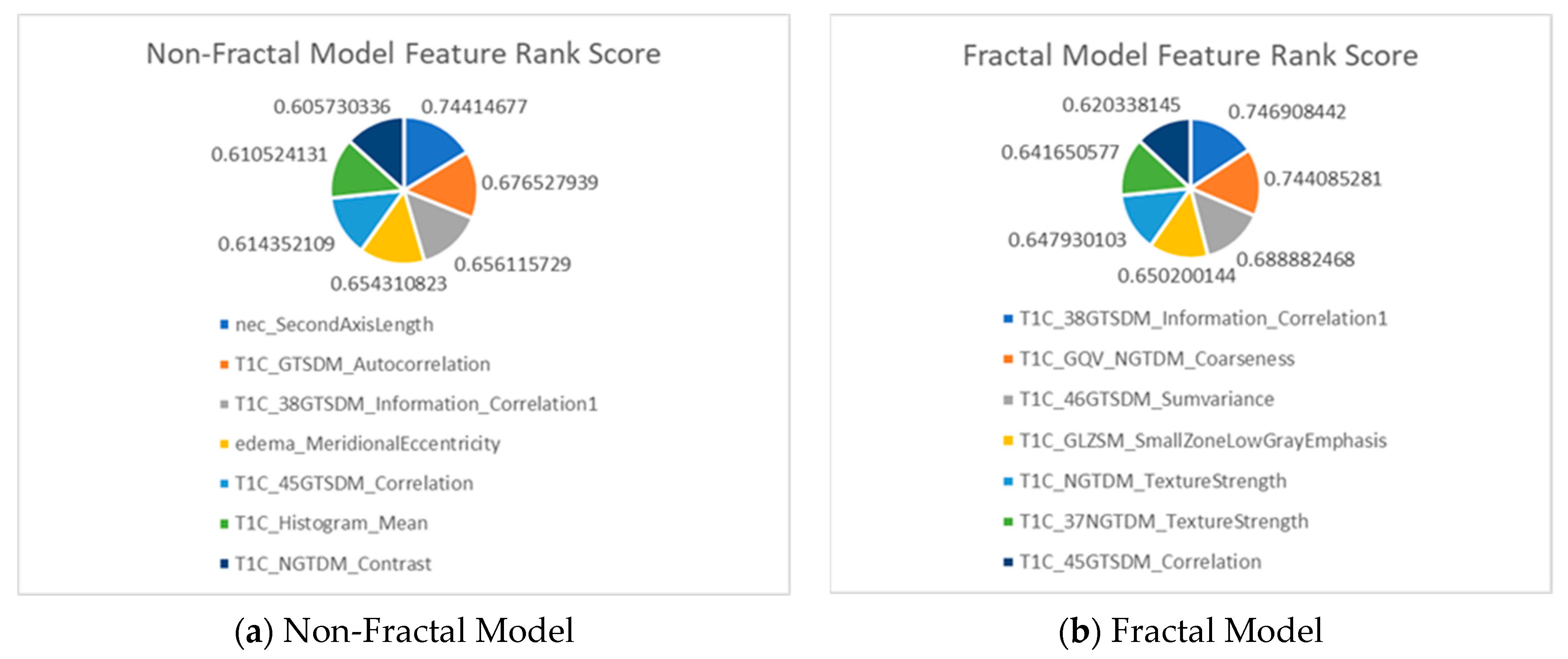
2.4. Selection of Radiomics Features and Model Building
2.5. Survival Analysis Modeling under Dependent Censoring
2.6. Survival Prediction
3. Results
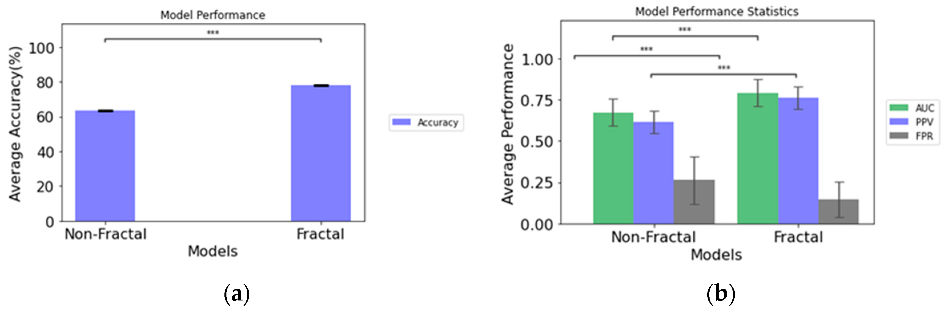
3.1. Predictive Performance of Rapid Early Progression (REP) Classification
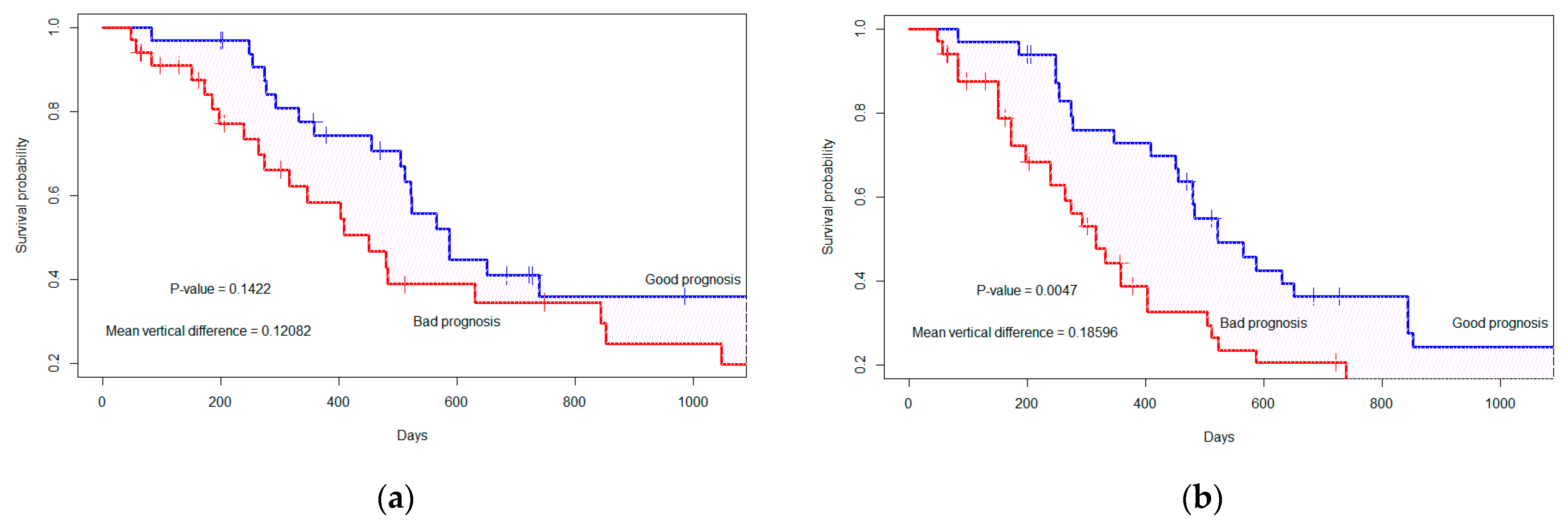
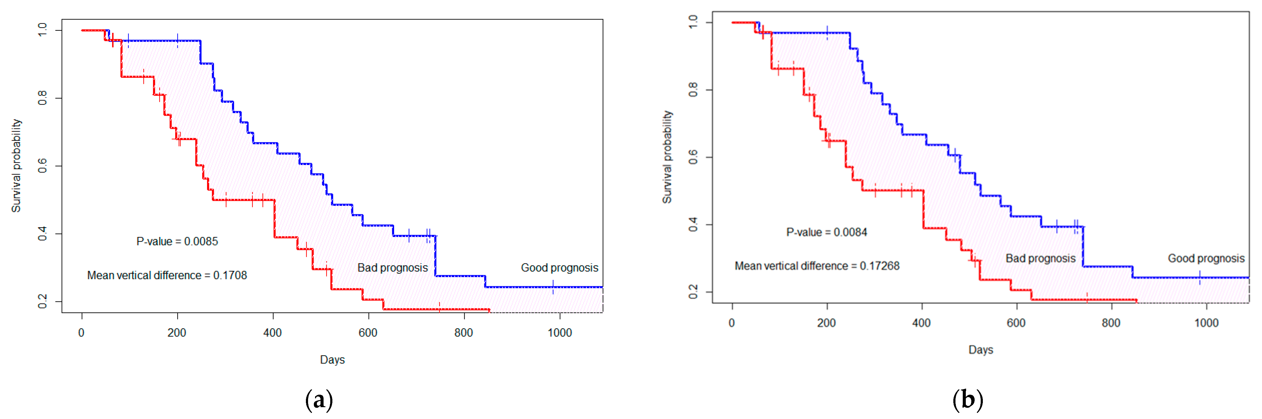
3.2. Survival Probability Analysis under Dependent Censoring
(2.46 × T1C_ptpsa_GLZSM_LargeZoneLowGrayEmphasis).
3.3. Binary Prediction of Survival
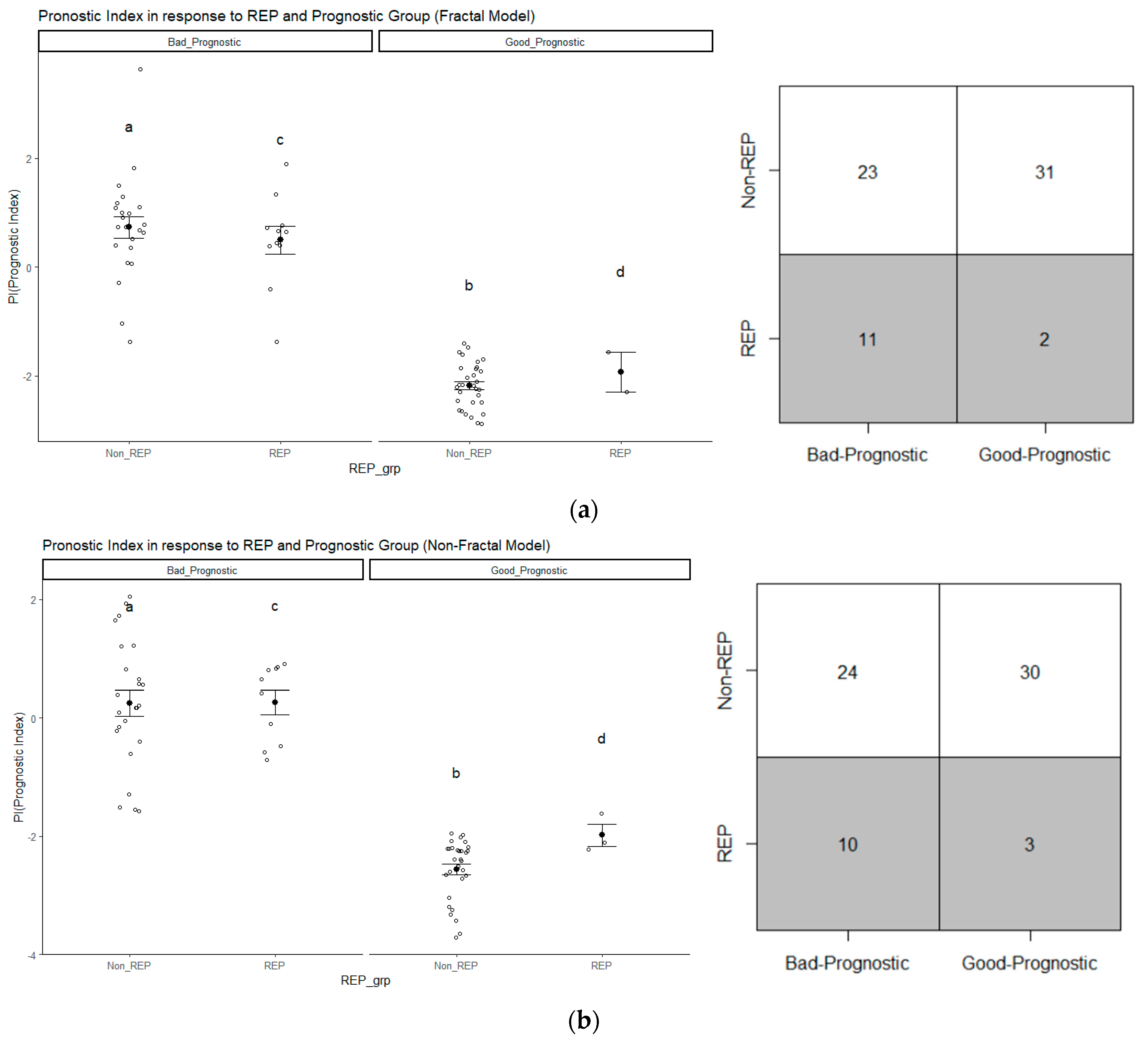
3.4. Analysis of Prognostic Groups and Its Association with REP Status
4. Discussion
5. Conclusions
Author Contributions
Funding
Institutional Review Board Statement
Informed Consent Statement
Data Availability Statement
Acknowledgments
Conflicts of Interest
Appendix A
| Algorithm A1: Subject Independent random sampling with i iteration for feature ranking. |
| 1: Input: total iteration number I, number of folds n, Radiomics feature data frame D, data frame with REP status Dp, data frame with non-REP status DN 2: Define SN as 20 patients randomly sampled from 57 non-REP DN in each iteration i, Sp 13 patients with REP status in each iteration i 3: Define Y as target class vector and j=1 to k the feature matrix in the data frame D, k is number of total features. 4: for iteration I = 1 to I do 5: Initialize SN  DN, randomly sample 20 patients from 57 non-REP patients. DN, randomly sample 20 patients from 57 non-REP patients.6: Initialize SP = DP 7: Initialize D = {DN, DP} 8: Save D after each ith iteration 9: within D split the target variable vector y and feature variable matrix as j=1 to k 10: for fold = 1 to n do 11: enumerate train and test indices for nth-fold in j=1 to k and y 12: for j = 1 to k do 13: fit a DTon the train indices of 14: predict ŷ on the test indices of 15: calculate F1-score based on true y and predicted ŷ of the test indices of 16: assign the score as the feature score of each 17: end for 18: end for 19: Output: Cumulative F1-score after n-fold cross-validation 20: end for 21: Output: Ranked features based on cumulative score after I iterations |
Appendix A.1. Model Building Algorithm
| Algorithm A2: Subject independent n-fold cross-validation with i iteration for model evaluation. |
| 1: Input: D after each i iterations, ranking score R for each feature in matrix j=1 to k 2: Define {XS} selected feature matrix based on R which is a subset of j=1 to k, Classification model C, Model performance evaluation metrics P 3: for iteration = 1 to I do 4: Initialize D = {DN, DP} 5: Initialize {XS} based on R and target vector y from D 6: for fold = 1 to n do 7: enumerate train and test index for n-fold in {XS} and y 8: fit classifier model C to the train index of {XS} and y 9: evaluate C on the test index of {XS} 10: Save P after each n 11: end for 12: Output: Cumulative P after n fold 13: end for 14: Output: Mean values of P after I iterations |

| Original Extracted Features for Non-Fractal Model | Significant (p-Value < 0.05) Features from Second-Step Feature Selection (Rank Score) |
|---|---|
| 41 texture features extracted from raw T1C |
|
| 12 volumetric features | None |
| 9 area-related features |
|
| 6 histogram statistics | None |
| Original Extracted Features for Fractal Model | Significant (p-Value < 0.05) Features from Second-Step Feature Selection (Rank Score) |
|---|---|
| 41 texture features extracted from PTPSA, mBm and GmBm of T1C (fractal features) |
|
| 41 texture features extracted from raw T1C |
|
| 12 volumetric features | None |
| 9 area-related features | None |
| 6 histogram statistics | None |
Appendix A.2. Detailed Statistical Analysis of Selected Features
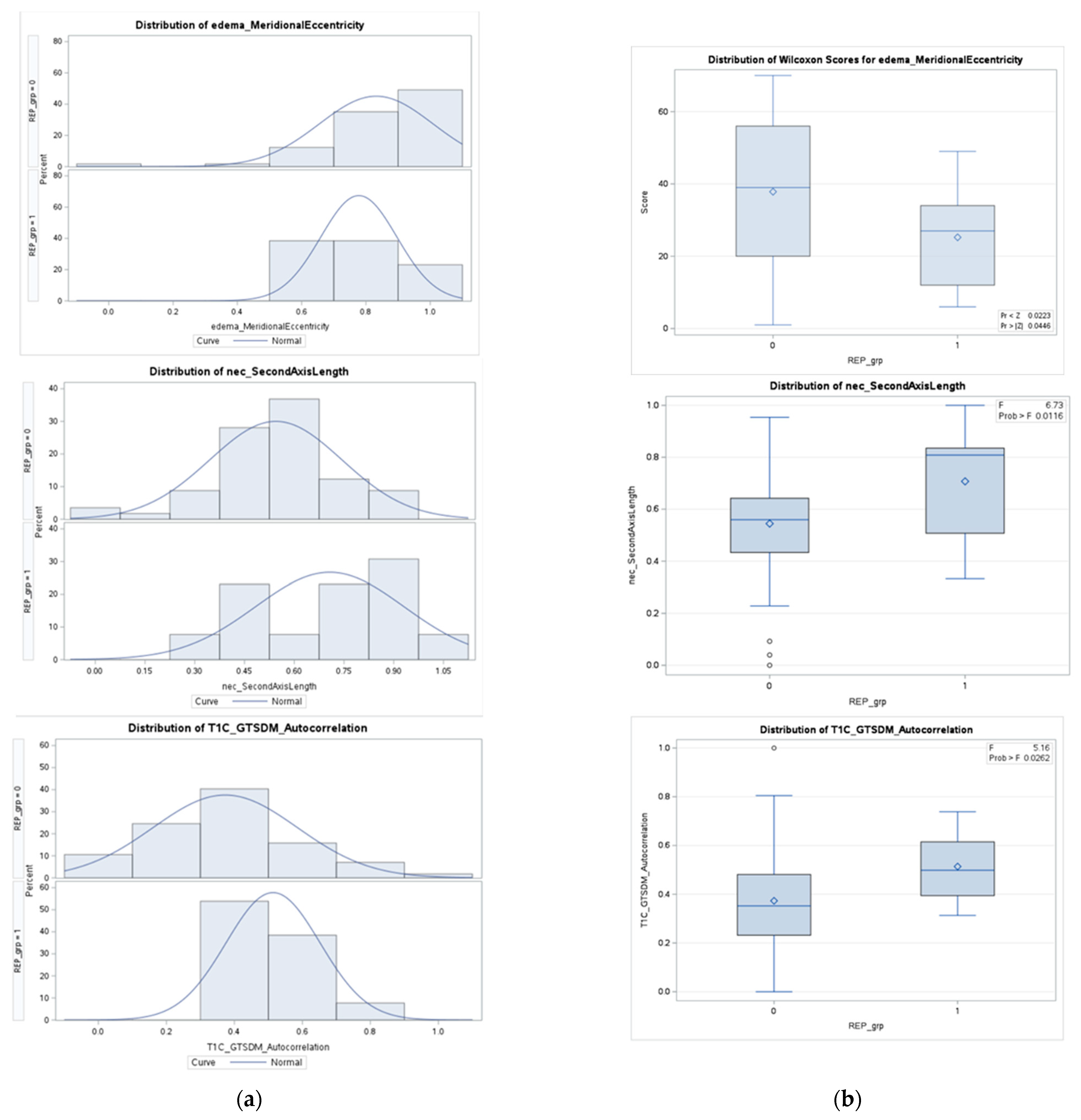

| Non-REP (n = 57) | REP (n = 13) | p-Value | |
|---|---|---|---|
| Eccentricity in edema region | 0.0446 | ||
| Mean (±std) | 0.8320 ± 0.1771 | 0.7779 ± 0.1184 | |
| Standard error | 0.0235 | 0.0328 | |
| Median | 0.8922 | 0.8109 | |
| Second axis (y-axis) length in necrosis region | 0.0116 | ||
| Mean (±std) | 0.5445 ± 0.1995 | 0.7072 ± 0.2239 | |
| Standard error | 0.0264 | 0.0621 | |
| Median | 0.5597 | 0.8085 | |
| Autocorrelation of GTSDM from T1C | 0.0262 | ||
| Mean (±std) | 0.3731 ± 0.2125 | 0.5137 ± 0.1381 | |
| Standard error | 0.0281 | 0.0383 | |
| Median | 0.3522 | 0.4984 |
| Non-REP (n = 57) | REP (n = 13) | p-Value | |
|---|---|---|---|
| GmBm * of T1C | 0.0296 | ||
| Mean (±std) | 0.3587 ± 0.2012 | 0.2372 ± 0.1272 | |
| Standard error | 0.0267 | 0.0353 | |
| Median | 0.3325 | 0.1918 | |
| Strength of NGTDM from 37th direction of T1C | 0.0019 | ||
| Mean (±std) | 1.9390 ± 0.5780 | 0.8260 ± 0.4864 | |
| Standard error | 0.0415 | 0.1349 | |
| Median | 1.2292 | 0.6970 | |
| Strength of NGTDM | 0.0013 | ||
| Mean (±std) | 0.1224 ± 0.0665 | 0.0389 ± 0.0299 | |
| Standard error | 0.0221 | 0.0083 | |
| Median | 0.0752 | 0.0252 |
Appendix B

| Features Name | Coefficient | p-Value |
|---|---|---|
| T1C_mBm_GLZSM_LargeZoneLowGrayEmphasis 1 | 5.46 | 0.002 |
| T1C_ptpsa_GLZSM_LargeZoneLowGrayEmphasis 2 | 2.46 | 0.038 |
| Fractal Model | Non-Fractal Model | |
|---|---|---|
| Feature Numbers | Difference in Survival Curves (p-Value *) | Difference in Survival Curves (p-Value *) |
| 3 | 0.261 (0.0001) | 0.198 (0.003) |
| 5 | 0.168 (0.010) | 0.161 (0.013) |
| 7 | 0.169 (0.009) | 0.173 (0.007) |
| 9 | 0.183 (0.004) | 0.128 (0.039) |
| 10 | 0.169 (0.008) | 0.127 (0.04) |
References
- Miller, K.D.; Ostrom, Q.T.; Kruchko, C.; Patil, N.; Tihan, T.; Cioffi, G.; Fuchs, H.E.; Waite, K.A.; Jemal, A.; Siegel, R.L.; et al. Brain and Other Central Nervous System Tumor Statistics, 2021. CA Cancer J. Clin. 2021, 71, 381–406. [Google Scholar] [CrossRef]
- Nam, J.Y.; de Groot, J.F. Treatment of Glioblastoma. J. Oncol. Pract. 2017, 13, 629–638. [Google Scholar] [CrossRef]
- Stupp, R.; Taillibert, S.; Kanner, A.; Read, W.; Steinberg, D.M.; Lhermitte, B.; Toms, S.; Idbaih, A.; Ahluwalia, M.S.; Fink, K.; et al. Effect of Tumor-Treating Fields Plus Maintenance Temozolomide vs Maintenance Temozolomide Alone on Survival in Patients With Glioblastoma: A Randomized Clinical Trial. JAMA 2017, 318, 2306–2316. [Google Scholar] [CrossRef] [PubMed]
- Majós, C.; Cos, M.; Castañer, S.; Pons, A.; Gil, M.; Fernández-Coello, A.; Maciá, M.; Bruna, J.; Aguilera, C. Preradiotherapy MR Imaging: A Prospective Pilot Study of the Usefulness of Performing an MR Examination Shortly before Radiation Therapy in Patients with Glioblastoma. Am. J. Neuroradiol. 2016, 37, 2224–2230. [Google Scholar] [CrossRef] [PubMed]
- Pirzkall, A.; McGue, C.; Saraswathy, S.; Cha, S.; Liu, R.; Vandenberg, S.; Lamborn, K.R.; Berger, M.S.; Chang, S.M.; Nelson, S.J. Tumor Regrowth between Surgery and Initiation of Adjuvant Therapy in Patients with Newly Diagnosed Glioblastoma. Neuro. Oncol. 2009, 11, 842–852. [Google Scholar] [CrossRef] [PubMed]
- Farace, P.; Amelio, D.; Ricciardi, G.K.; Zoccatelli, G.; Magon, S.; Pizzini, F.; Alessandrini, F.; Sbarbati, A.; Amichetti, M.; Beltramello, A. Early MRI Changes in Glioblastoma in the Period between Surgery and Adjuvant Therapy. J. Neurooncol. 2013, 111, 177–185. [Google Scholar] [CrossRef]
- Palmer, J.D.; Bhamidipati, D.; Shukla, G.; Sharma, D.; Glass, J.; Kim, L.; Evans, J.J.; Judy, K.; Farrell, C.; Andrews, D.W.; et al. Rapid Early Tumor Progression Is Prognostic in Glioblastoma Patients. Am. J. Clin. Oncol. Cancer Clin. Trials 2019, 42, 481–486. [Google Scholar] [CrossRef]
- Lakomy, R.; Kazda, T.; Selingerova, I.; Poprach, A.; Pospisil, P.; Belanova, R.; Fadrus, P.; Smrcka, M.; Vybihal, V.; Jancalek, R.; et al. Pre-Radiotherapy Progression after Surgery of Newly Diagnosed Glioblastoma: Corroboration of New Prognostic Variable. Diagnostics 2020, 10, 676. [Google Scholar] [CrossRef]
- NCCN Guidelines. NCCN Guidelines for Treatment of Cancer by Site. Central Nervous System Cancers. National Comprehensive Cancer Network. Available online: https://www.nccn.org/guidelines/category_1#cns (accessed on 21 February 2023).
- Kazerooni, A.F.; Bagley, S.J.; Akbari, H.; Saxena, S.; Bagheri, S.; Guo, J.; Chawla, S.; Nabavizadeh, A.; Mohan, S.; Bakas, S.; et al. Applications of Radiomics and Radiogenomics in High-Grade Gliomas in the Era of Precision Medicine. Cancers 2021, 13, 5921. [Google Scholar] [CrossRef]
- Mulford, K.; McMahon, M.; Gardeck, A.M.; Hunt, M.A.; Chen, C.C.; Odde, D.J.; Wilke, C. Predicting Glioblastoma Cellular Motility from In Vivo MRI with a Radiomics Based Regression Model. Cancers 2022, 14, 578. [Google Scholar] [CrossRef]
- Cepeda, S.; Pérez-Nuñez, A.; García-García, S.; García-Pérez, D.; Arrese, I.; Jiménez-Roldán, L.; García-Galindo, M.; González, P.; Velasco-Casares, M.; Zamora, T.; et al. Predicting Short-Term Survival after Gross Total or near Total Resection in Glioblastomas by Machine Learning-Based Radiomic Analysis of Preoperative Mri. Cancers 2021, 13, 5047. [Google Scholar] [CrossRef] [PubMed]
- Pereira, S.; Pinto, A.; Alves, V.; Silva, C.A. Brain Tumor Segmentation Using Convolutional Neural Networks in MRI Images. IEEE Trans. Med. Imaging 2016, 35, 1240–1251. [Google Scholar] [CrossRef] [PubMed]
- Pei, L.; Vidyaratne, L.; Rahman, M.M.; Iftekharuddin, K.M. Context Aware Deep Learning for Brain Tumor Segmentation, Subtype Classification, and Survival Prediction Using Radiology Images. Sci. Rep. 2020, 10, 19726. [Google Scholar] [CrossRef] [PubMed]
- Shboul, Z.A.; Chen, J.; Iftekharuddin, K.M. Prediction of Molecular Mutations in Diffuse Low-Grade Gliomas Using MR Imaging Features. Sci. Rep. 2020, 10, 3711. [Google Scholar] [CrossRef]
- Emura, T.; Chen, Y.-H. Analysis of Survival Data with Dependent Censoring Copula-Based Approaches; Springer: Singapore, 2018; ISBN 9789811071638. [Google Scholar]
- Emura, T.; Chen, Y.H. Gene Selection for Survival Data under Dependent Censoring: A Copula-Based Approach. Stat. Methods Med. Res. 2016, 25, 2840–2857. [Google Scholar] [CrossRef]
- Waqar, M.; Trifiletti, D.M.; McBain, C.; O’Connor, J.; Coope, D.J.; Akkari, L.; Quinones-Hinojosa, A.; Borst, G.R. Early Therapeutic Interventions for Newly Diagnosed Glioblastoma: Rationale and Review of the Literature. Curr. Oncol. Rep. 2022, 24, 311–324. [Google Scholar] [CrossRef]
- Waqar, M.; Roncaroli, F.; Lehrer, E.J.; Palmer, J.D.; Villanueva-meyer, J.; Braunstein, S.; Hall, E.; Aznar, M.; Hamer, P.C.D.W.; Urso, P.I.D.; et al. Rapid early progression (REP) of glioblastoma is an independent negative prognostic factor: Results from a systematic review and meta-analysis. Neuro-Oncol. Adv. 2022, 4, vdac075. [Google Scholar] [CrossRef]
- Smith, S.M.; Jenkinson, M.; Woolrich, M.W.; Beckmann, C.F.; Behrens, T.E.J.; Johansen-Berg, H.; Bannister, P.R.; De Luca, M.; Drobnjak, I.; Flitney, D.E.; et al. Advances in Functional and Structural MR Image Analysis and Implementation as FSL. Neuroimage 2004, 23 (Suppl. 1), S208–S219. [Google Scholar] [CrossRef]
- Smith, S.M. Fast Robust Automated Brain Extraction. Hum. Brain Mapp. 2002, 17, 143–155. [Google Scholar] [CrossRef]
- Smith, S.M.; Brady, J.M. SUSAN—A New Approach to Low Level Image Processing. Int. J. Comput. Vis. 1997, 23, 45–78. [Google Scholar] [CrossRef]
- Sled, J.G.; Zijdenbos, A.P.; Evans, A.C. A Nonparametric Method for Automatic Correction of Intensity Nonuniformity in MRI Data. IEEE Trans. Med. Imaging 1998, 17, 87–97. [Google Scholar] [CrossRef] [PubMed]
- Menze, B.H.; Jakab, A.; Bauer, S.; Kalpathy-Cramer, J.; Farahani, K.; Kirby, J.; Burren, Y.; Porz, N.; Slotboom, J.; Wiest, R.; et al. The Multimodal Brain Tumor Image Segmentation Benchmark (BRATS). IEEE Trans. Med. Imaging 2015, 34, 1993–2024. [Google Scholar] [CrossRef] [PubMed]
- Baid, U.; Ghodasara, S.; Bilello, M.; Mohan, S.; Calabrese, E.; Colak, E.; Farahani, K.; Kalpathy-Cramer, J.; Kitamura, F.C.; Pati, S.; et al. The RSNA-ASNR-MICCAI BraTS 2021 Benchmark on Brain Tumor Segmentation and Radiogenomic Classification. arXiv 2021, arXiv:2107.02314. [Google Scholar]
- Bakas, S.; Akbari, H.; Sotiras, A.; Bilello, M.; Rozycki, M.; Kirby, J.S.; Freymann, J.B.; Farahani, K.; Davatzikos, C. Advancing The Cancer Genome Atlas Glioma MRI Collections with Expert Segmentation Labels and Radiomic Features. Sci. Data 2017, 4, 2017–2018. [Google Scholar] [CrossRef]
- Iftekharuddin, K.M.; Jia, W.; Marsh, R. Fractal Analysis of Tumor in Brain MR Images. Mach. Vis. Appl. 2003, 13, 352–362. [Google Scholar] [CrossRef]
- Reza, S.M.S.; Mays, R.; Iftekharuddin, K.M. Multi-Fractal Detrended Texture Feature for Brain Tumor Classification. In Proceedings of the Medical Imaging 2015: Computer-Aided Diagnosis, Orlando, FL, USA, 21–26 February 2015; Volume 9414. [Google Scholar]
- Ayache, A.; Véhel, J.L. On the Identification of the Pointwise Hölder Exponent of the Generalized Multifractional Brownian Motion. Stoch. Process. Their Appl. 2004, 111, 119–156. [Google Scholar] [CrossRef]
- John, P. Brain Tumor Classification Using Wavelet and Texture Based Neural Network. Int. J. Sci. Eng. Res. 2012, 3, 1–7. [Google Scholar]
- Vallières, M.; Freeman, C.R.; Skamene, S.R.; El Naqa, I. A Radiomics Model from Joint FDG-PET and MRI Texture Features for the Prediction of Lung Metastases in Soft-Tissue Sarcomas of the Extremities. Phys. Med. Biol. 2015, 60, 5471–5496. [Google Scholar] [CrossRef]
- Farzana, W.; Shboul, Z.A.; Temtam, A.; Iftekharuddin, K.M. Uncertainty Estimation in Classification of MGMT Using Radiogenomics for Glioblastoma Patients. In Proceedings of the Medical Imaging 2022: Computer-Aided Diagnosis, San Diego, CA, USA, 4 April 2022; Volume 12033, p. 51. [Google Scholar]
- Wong, T.T.; Yeh, P.Y. Reliable Accuracy Estimates from K-Fold Cross Validation. IEEE Trans. Knowl. Data Eng. 2020, 32, 1586–1594. [Google Scholar] [CrossRef]
- Emura, T.; Chen, Y.H.; Chen, H.Y. Survival Prediction Based on Compound Covariate under Cox Proportional Hazard Models. PLoS ONE 2012, 7, e47627. [Google Scholar] [CrossRef]
- Emura, T.; Matsui, S.; Chen, H.Y. Compound.Cox: Univariate Feature Selection and Compound Covariate for Predicting Survival. Comput. Methods Programs Biomed. 2019, 168, 21–37. [Google Scholar] [CrossRef] [PubMed]
- Chen, Y.-H. Semiparametric Marginal Regression Analysis for Dependent Competing Risks under an Assumed Copula. J. R. Stat. Soc. Ser. B Stat. Methodol. 2010, 72, 235–251. [Google Scholar] [CrossRef]
- Rivest, L.-P.; Wells, M.T. A Martingale Approach to the Copula-Graphic Estimator for the Survival Function under Dependent Censoring. J. Multivar. Anal. 2001, 79, 138–155. [Google Scholar] [CrossRef]
- Pepe, M.S.; Fleming, T.R. Weighted Kaplan-Meier Statistics: A Class of Distance Tests for Censored Survival Data. Biometrics 1989, 45, 497–507. [Google Scholar] [CrossRef]
- Frankel, P.H.; Reid, M.E.; Marshall, J.R. A Permutation Test for a Weighted Kaplan-Meier Estimator with Application to the Nutritional Prevention of Cancer Trial. Contemp. Clin. Trials 2007, 28, 343–347. [Google Scholar] [CrossRef]
- Houdova Megova, M.; Drábek, J.; Dwight, Z.; Trojanec, R.; Koudeláková, V.; Vrbková, J.; Kalita, O.; Mlcochova, S.; Rabcanova, M.; Hajdúch, M. Isocitrate Dehydrogenase Mutations Are Better Prognostic Marker than O6-Methylguanine-DNA Methyltransferase Promoter Methylation in Glioblastomas—A Retrospective, Single-Centre Molecular Genetics Study of Gliomas. Klin. Onkol. 2017, 30, 361–371. [Google Scholar] [CrossRef]
- Killela, P.J.; Pirozzi, C.J.; Healy, P.; Reitman, Z.J.; Lipp, E.; Rasheed, B.A.; Yang, R.; Diplas, B.H.; Wang, Z.; Greer, P.K.; et al. Mutations in IDH1, IDH2, and in the TERT Promoter Define Clinically Distinct Subgroups of Adult Malignant Gliomas. Oncotarget 2014, 5, 1515–1525. [Google Scholar] [CrossRef]
- Bakas, S.; Reyes, M.; Jakab, A.; Bauer, S.; Rempfler, M.; Crimi, A.; Shinohara, R.T.; Berger, C.; Ha, S.M.; Rozycki, M.; et al. Identifying the Best Machine Learning Algorithms for Brain Tumor Segmentation, Progression Assessment, and Overall Survival Prediction in the BRATS Challenge. arXiv 2018, arXiv:1811.02629. [Google Scholar]
- Baine, M.; Burr, J.; Du, Q.; Zhang, C.; Liang, X.; Krajewski, L.; Zima, L.; Rux, G.; Zhang, C.; Zheng, D. The Potential Use of Radiomics with Pre-Radiation Therapy Mr Imaging in Predicting Risk of Pseudoprogression in Glioblastoma Patients. J. Imaging 2021, 7, 17. [Google Scholar] [CrossRef]
- Lohmann, P.; Elahmadawy, M.A.; Gutsche, R.; Werner, J.M.; Bauer, E.K.; Ceccon, G.; Kocher, M.; Lerche, C.W.; Rapp, M.; Fink, G.R.; et al. Fet Pet Radiomics for Differentiating Pseudoprogression from Early Tumor Progression in Glioma Patients Post-chemoradiation. Cancers 2020, 12, 3835. [Google Scholar] [CrossRef]
- Chiu, F.Y.; Yen, Y. Efficient Radiomics-Based Classification of Multi-Parametric MR Images to Identify Volumetric Habitats and Signatures in Glioblastoma: A Machine Learning Approach. Cancers 2022, 14, 1475. [Google Scholar] [CrossRef]
- Yoon, H.G.; Cheon, W.; Jeong, S.W.; Kim, H.S.; Kim, K.; Nam, H.; Han, Y.; Lim, D.H. Multi-Parametric Deep Learning Model for Prediction of Overall Survival after Postoperative Concurrent Chemoradiotherapy in Glioblastoma Patients. Cancers 2020, 12, 2284. [Google Scholar] [CrossRef]
- Kohavi, R. A Study of Cross-Validation and Bootstrap for Accuracy Estimation and Model Selection. In Proceedings of the 1995 International Joint Conference on Artificial Intelligence, Montreal, QC, Canada, 20–25 August 1995. [Google Scholar]
- Kamalov, F.; Thabtah, F.; Leung, H.H. Feature Selection in Imbalanced Data. Ann. Data Sci. 2022. [Google Scholar] [CrossRef]
- Cox, D.R. Regression Models and Life-Tables. J. R. Stat. Soc. Ser. B 1972, 34, 187–220. [Google Scholar] [CrossRef]
- Weber, E.M.; Andrew, C.T. Quantifying the association between progression-free survival and overall survival in oncology trials using Kendall’s τ. Stat. Med. 2019, 38, 703–719. [Google Scholar] [CrossRef] [PubMed]
- Harrell, F.E.; Califf, R.M.; Pryor, D.B.; Lee, K.L.; Rosati, R.A. Evaluating the Yield of Medical Tests. JAMA J. Am. Med. Assoc. 1982, 247, 2543–2546. [Google Scholar] [CrossRef]
- Harrell, F.E.; Lee, K.L.; Mark, D.B. Multivariable Prognostic Models: Issues in Developing Models, Evaluating Assumptions and Adequacy, and Measuring and Reducing Errors. Stat. Med. 1996, 15, 361–387. [Google Scholar] [CrossRef]
- Schweizer, B. Introduction to Copulas. J. Hydrol. Eng. 2007, 12, 346. [Google Scholar] [CrossRef]


| Total (n = 70) | REP (n = 13) | Non-REP (n = 57) | |
|---|---|---|---|
| Survival Days from Surgery | |||
| Present (patient dead/expired) | 45 | 8 | 37 |
| Lost follow-up (censored) * | 22 | 5 | 17 |
| Not dead nor censored | 3 | 0 | 3 |
| MGMT Promoter Status | |||
| Hypermethylated | 23 | 5 | 18 |
| Unmethylated | 33 | 6 | 27 |
| Indeterminate | 14 | 2 | 12 |
| IDH-1 Mutation Status | |||
| Wild type | 59 | 12 | 47 |
| Mutant | 8 | 1 | 7 |
| Indeterminate | 3 | 0 | 3 |
| 1p-19q-Codeletion Status | |||
| Codeletion | 2 | 0 | 2 |
| Negative | 18 | 1 | 17 |
| Indeterminate | 50 | 12 | 38 |
| Expired/Dead (Denoted as 1) | Alive (Denoted as 0) | |
|---|---|---|
| Non-Censored Patients (n = 45) | 45 | None |
| Censored/Lost Follow-up Patients (n = 22) | 9 | 13 |
| Model Configurations | Area under Curve (AUC) | Accuracy (%) | Positive Predictive Value (PPV) | False Positive Rate (FPR) |
|---|---|---|---|---|
| Non-Fractal Model | 0.673 ± 0.082 | 63.5 ± 0.069 | 0.617 ± 0.067 | 0.262 ± 0.177 |
| Fractal Model | 0.793 ± 0.082 | 78.1 ± 0.071 | 0.761 ± 0.069 | 0.145 ± 0.107 |
| Fractal Model Features | ||
| Features Name | Co-Efficient | p-Value |
| ET2 1 | −1.58 | 0.0045 |
| T1C_ptpsa_GLZSM_Low_Gray_Level_Zone_Emphasis | 1.33 | 0.0110 |
| L2_Orientation 2 | 0.74 | 0.0183 |
| edema_FirstAxisLength 3 | −0.91 | 0.0194 |
| wt_MajorAxisLength 4 | −0.93 | 0.0198 |
| L1_Extent 2 | 0.76 | 0.0218 |
| L3_Orientation 2 | 0.70 | 0.0261 |
| T1C_mBm_GLZSM_LargeZoneLowGrayEmphasis | 2.27 | 0.0316 |
| nec_SecondAxis_1 5 | −1.06 | 0.0355 |
| T1C_ED_Histogram_Mean 6 | 1.09 | 0.0434 |
| Non-Fractal Model Features | ||
| Features Name | Co-Efficient | p-Value |
| ET2 1 | −1.58 | 0.0045 |
| L2_Orientation 2 | 0.74 | 0.0183 |
| edema_FirstAxisLength 3 | −0.91 | 0.0194 |
| wt_MajorAxisLength 4 | −0.93 | 0.0198 |
| L1_Extent 2 | 0.76 | 0.0218 |
| L3_Orientation 2 | 0.70 | 0.0261 |
| nec_SecondAxis_1 | −1.06 | 0.0355 |
| T1C_ED_Histogram_Mean 6 | 1.09 | 0.0434 |
| ED_up_left_y * | 0.83 | 0.0585 |
| T1C_ED_Histogram_Skewness * | −1.18 | 0.0718 |
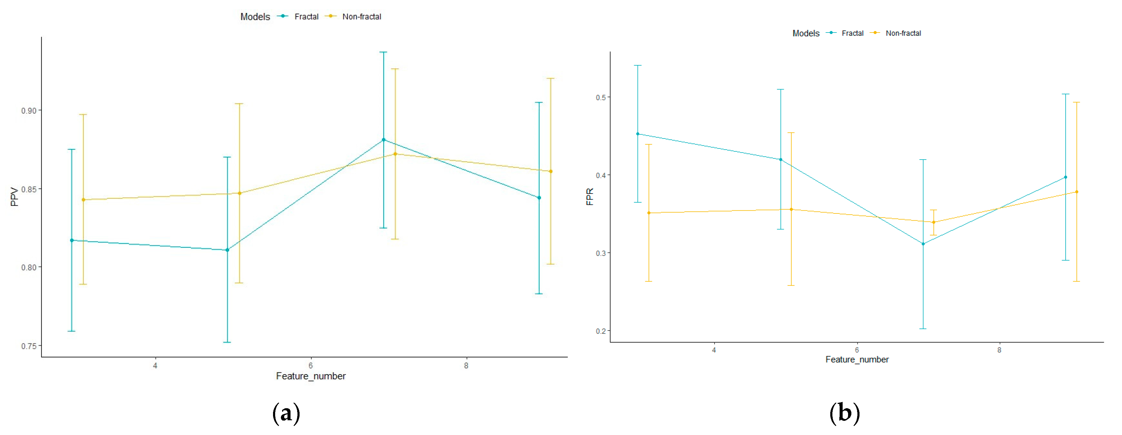
| Number of Features | Model Configurations | Area under Curve (AUC) | Accuracy (%) | Positive Predicted Value (PPV) | False Positive Rate (FPR) |
|---|---|---|---|---|---|
| Top 3 features | Non-Fractal Model | 0.730 ± 0.235 | 74.018 ± 0.045 | 0.843 ± 0.054 | 0.351 ± 0.088 |
| Fractal Model | 0.659 ± 0.241 | 67.67 ± 0.040 | 0.817 ± 0.058 | 0.453 ± 0.088 | |
| Top 5 features | Non-Fractal Model | 0.783 ± 0.199 | 73.22 ± 0.048 | 0.847 ± 0.057 | 0.356 ± 0.098 |
| Fractal Model | 0.658 ± 0.243 | 70.03 ± 0.048 | 0.811 ± 0.059 | 0.420 ± 0.090 | |
| Top 7 features | Non-Fractal Model | 0.735 ± 0.219 | 73.05 ± 0.045 | 0.872 ± 0.054 | 0.339 ± 0.106 |
| Fractal Model | 0.762 ± 0.214 | 74.39 ± 0.046 | 0.881 ± 0.056 | 0.311 ± 0.109 | |
| Top 9 features | Non-Fractal Model | 0.725 ± 0.224 | 71.00 ± 0.049 | 0.861 ± 0.059 | 0.378 ± 0.115 |
| Fractal Model | 0.719 ± 0.214 | 70.37 ± 0.048 | 0.844 ± 0.061 | 0.397 ± 0.107 |
| Model Configurations | Area under Curve | Accuracy (%) | Positive Predictive Value (PPV) | False Positive Rate (FPR) |
|---|---|---|---|---|
| Non-Fractal Molecular | 0.757 ± 0.214 | 72.36 ± 0.046 | 0.866 ± 0.058 | 0.354 ± 0.109 |
| Fractal Molecular | 0.762 ± 0.214 | 73.48 ± 0.047 | 0.883 ± 0.057 | 0.322 ± 0.114 |
| Group Name | Number of Cases | Mean | Standard Deviation | Standard Error | Median | Range | p-Value |
|---|---|---|---|---|---|---|---|
| Bad Prognostic | 34 | 420.382 | 335.353 | 57.513 | 329.00 | 48.00–1211.00 | 0.02 |
| Good Prognostic | 33 | 678.424 | 494.209 | 86.031 | 511.00 | 57.00–1821.00 | |
| Non-REP | 54 | 604.259 | 441.961 | 60.143 | 474.50 | 48.00–1821.00 | 0.006 |
| REP | 13 | 311.615 | 340.626 | 94.472 | 172.00 | 57.00–1211.00 |
Disclaimer/Publisher’s Note: The statements, opinions and data contained in all publications are solely those of the individual author(s) and contributor(s) and not of MDPI and/or the editor(s). MDPI and/or the editor(s) disclaim responsibility for any injury to people or property resulting from any ideas, methods, instructions or products referred to in the content. |
© 2023 by the authors. Licensee MDPI, Basel, Switzerland. This article is an open access article distributed under the terms and conditions of the Creative Commons Attribution (CC BY) license (https://creativecommons.org/licenses/by/4.0/).
Share and Cite
Farzana, W.; Basree, M.M.; Diawara, N.; Shboul, Z.A.; Dubey, S.; Lockhart, M.M.; Hamza, M.; Palmer, J.D.; Iftekharuddin, K.M. Prediction of Rapid Early Progression and Survival Risk with Pre-Radiation MRI in WHO Grade 4 Glioma Patients. Cancers 2023, 15, 4636. https://doi.org/10.3390/cancers15184636
Farzana W, Basree MM, Diawara N, Shboul ZA, Dubey S, Lockhart MM, Hamza M, Palmer JD, Iftekharuddin KM. Prediction of Rapid Early Progression and Survival Risk with Pre-Radiation MRI in WHO Grade 4 Glioma Patients. Cancers. 2023; 15(18):4636. https://doi.org/10.3390/cancers15184636
Chicago/Turabian StyleFarzana, Walia, Mustafa M. Basree, Norou Diawara, Zeina A. Shboul, Sagel Dubey, Marie M. Lockhart, Mohamed Hamza, Joshua D. Palmer, and Khan M. Iftekharuddin. 2023. "Prediction of Rapid Early Progression and Survival Risk with Pre-Radiation MRI in WHO Grade 4 Glioma Patients" Cancers 15, no. 18: 4636. https://doi.org/10.3390/cancers15184636
APA StyleFarzana, W., Basree, M. M., Diawara, N., Shboul, Z. A., Dubey, S., Lockhart, M. M., Hamza, M., Palmer, J. D., & Iftekharuddin, K. M. (2023). Prediction of Rapid Early Progression and Survival Risk with Pre-Radiation MRI in WHO Grade 4 Glioma Patients. Cancers, 15(18), 4636. https://doi.org/10.3390/cancers15184636