
Self-Supervised Adversarial Learning with a Limited Dataset for Electronic Cleansing in Computed Tomographic Colonography: A Preliminary Feasibility Study


Abstract
Simple Summary
Abstract
1. Introduction
2. Materials and Methods
2.1. CTC Datasets
2.2. Extraction of Volumes of Interest (VOIs)
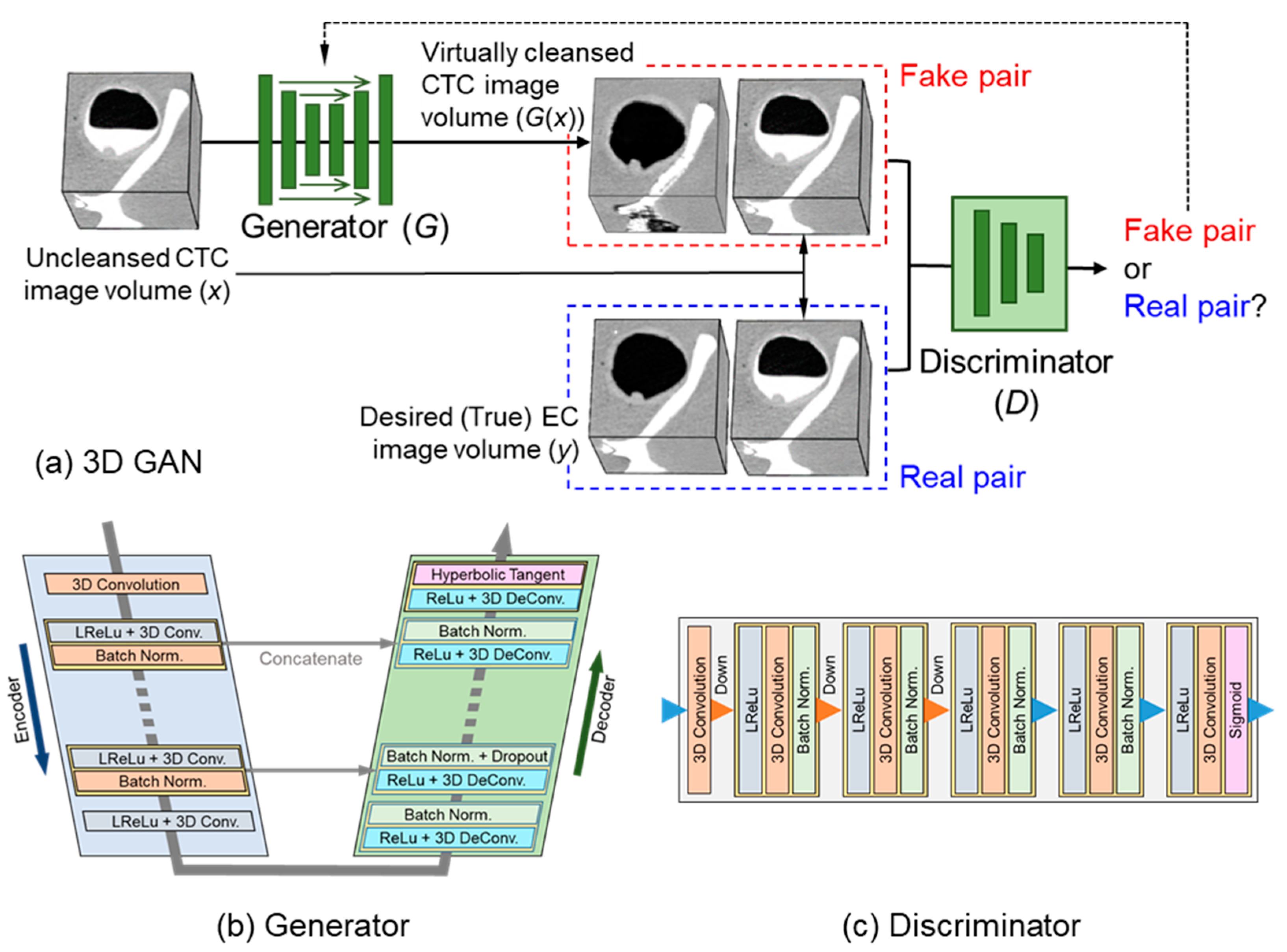
2.3. 3D GAN for EC
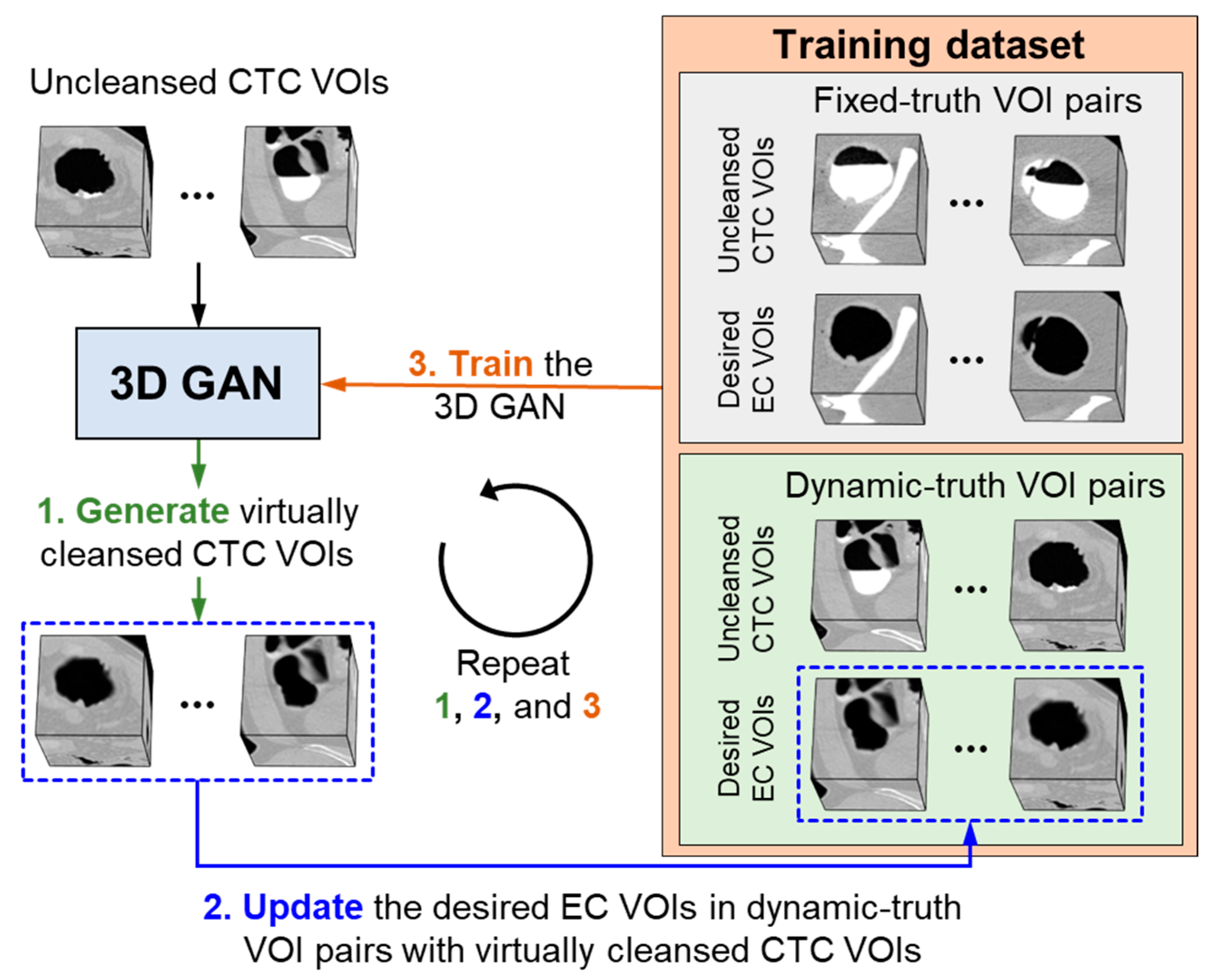
2.4. Self-Supervised Learning of 3D GAN
2.5. Implementation of the 3D-GAN EC Scheme
2.6. Evaluation Methods
2.6.1. Phantom Study: Objective Evaluation and Optimization of the 3D-GAN EC Scheme
2.6.2. Clinical Study: Evaluation of the Cleansing Quality in Clinical CTC Cases
3. Results
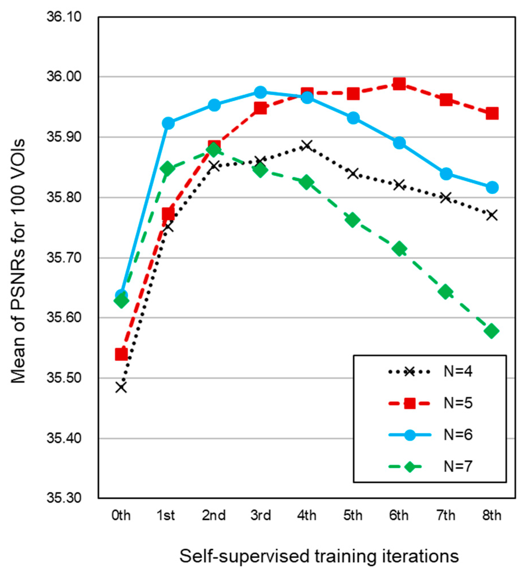
3.1. Phantom Study
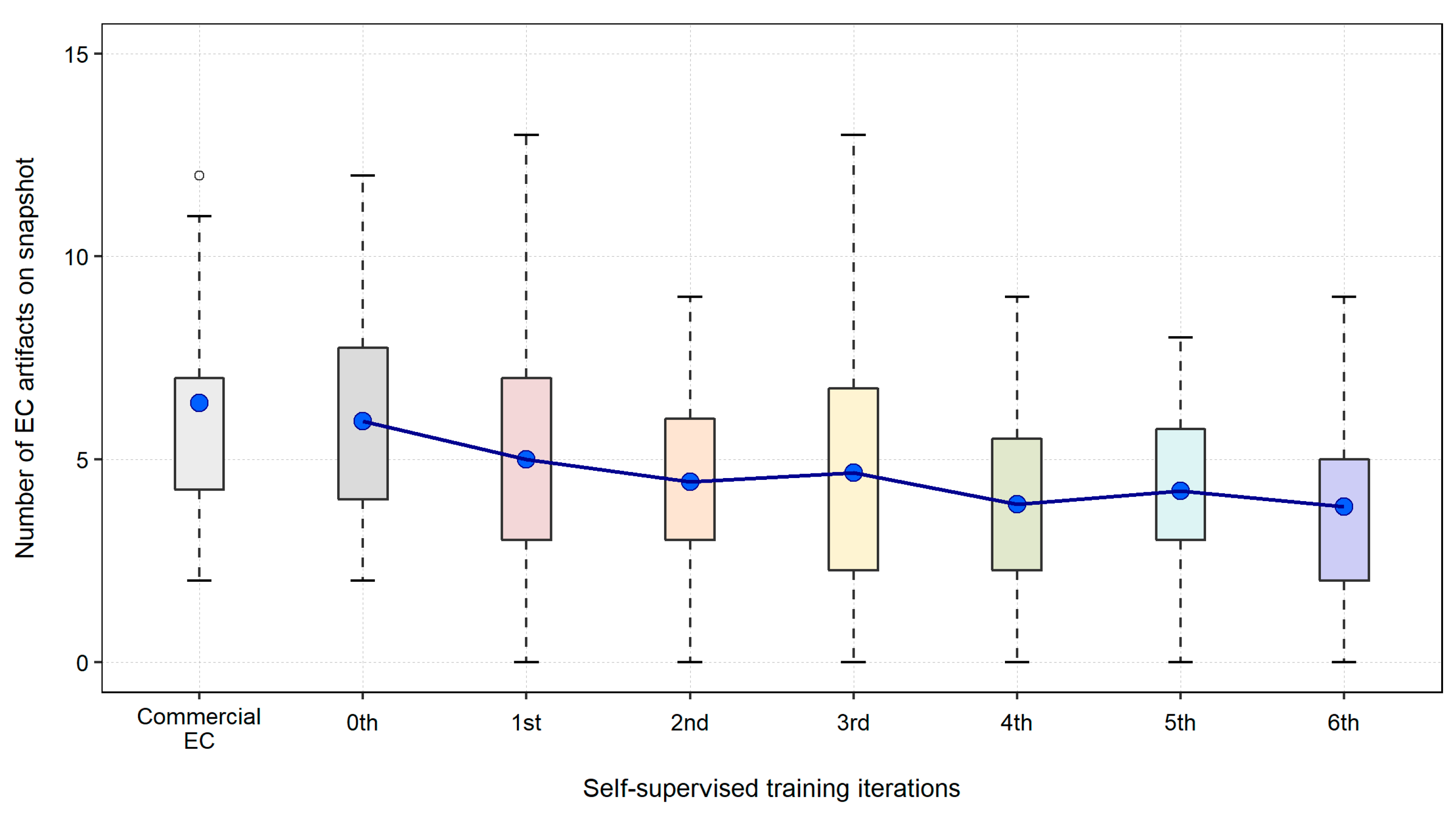
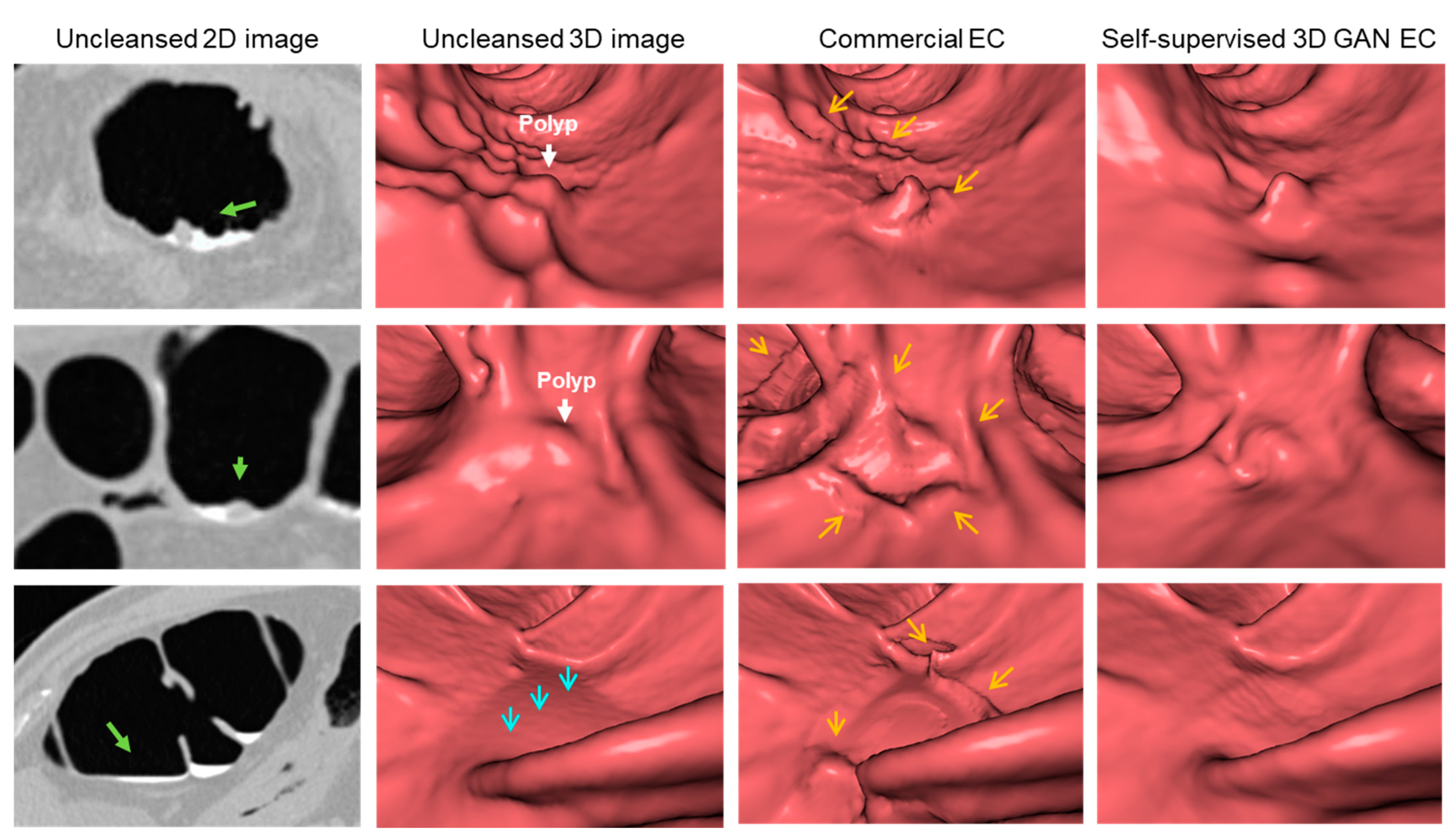
3.2. Clinical Study
4. Discussion
5. Conclusions
Author Contributions
Funding
Institutional Review Board Statement
Informed Consent Statement
Data Availability Statement
Acknowledgments
Conflicts of Interest
Appendix A

| Layers | Kernel | Stride | Padding | Output Shape | Activation | Batch Norm. | Dropout |
|---|---|---|---|---|---|---|---|
| Input: Image | 128 × 128 × 128 × 1 | ||||||
| Conv. Layer 1 | 4 | 2 | 1 | 64 × 64 × 64 × 64 | LeakyReLU | ||
| Conv. Layer 2 | 4 | 2 | 1 | 32 × 32 × 32 × 128 | LeakyReLU | True | |
| Conv. Layer 3 | 4 | 2 | 1 | 16 × 16 × 16 × 256 | LeakyReLU | True | |
| Conv. Layer 4 | 4 | 2 | 1 | 8 × 8 × 8 × 512 | LeakyReLU | True | |
| Conv. Layer 5 | 4 | 2 | 1 | 4 × 4 × 4 × 512 | LeakyReLU | True | |
| Conv. Layer 6 | 4 | 2 | 1 | 2 × 2 × 2 × 512 | LeakyReLU | True | |
| Conv. Layer 7 | 4 | 2 | 1 | 1 × 1 × 1 × 512 | ReLU | ||
| Deconv. Layer 8 | 4 | 2 | 1 | 2 × 2 × 2 × 512 | True | ||
| Concatenate (Layer 8, Layer 6) | |||||||
| Deconv. Layer 9 | 4 | 2 | 1 | 4 × 4 × 4 × 512 | ReLU | True | True |
| Concatenate (Layer 9, Layer 5) | |||||||
| Deconv. Layer 10 | 4 | 2 | 1 | 8 × 8 × 8 × 512 | ReLU | True | True |
| Concatenate (Layer 10, Layer 4) | |||||||
| Deconv. Layer 11 | 4 | 2 | 1 | 16 × 16 × 16 × 256 | ReLU | True | |
| Concatenate (Layer 11, Layer 3) | |||||||
| Deconv. Layer 12 | 4 | 2 | 1 | 32 × 32 × 32 × 128 | ReLU | True | |
| Concatenate (Layer 12, Layer 2) | |||||||
| Deconv. Layer 13 | 4 | 2 | 1 | 64 × 64 × 64 × 64 | ReLU | True | |
| Concatenate (Layer 13, Layer 1) | |||||||
| Deconv. Layer 14 | 4 | 2 | 1 | 128 × 128 × 128 × 1 | Tanh | ||
| Layers | Kernel | Stride | Padding | Output Shape | Activation | Batch Norm. |
|---|---|---|---|---|---|---|
| Input 1: Real Image | 128 × 128 × 128 × 1 | |||||
| Input 2: Fake Image | 128 × 128 × 128 × 1 | |||||
| Concatenate (Input 1, Input 2) | ||||||
| Conv. Layer 1 | 4 | 2 | 1 | 64 × 64 × 64 × 64 | LeakyReLU | |
| Conv. Layer 2 | 4 | 2 | 1 | 32 × 32 × 32 × 128 | LeakyReLU | True |
| Conv. Layer 3 | 4 | 2 | 1 | 16 × 16 × 16 × 256 | LeakyReLU | True |
| Conv. Layer 4 | 4 | 2 | 1 | 8 × 8 × 8 × 512 | LeakyReLU | True |
| Conv. Layer 5 | 4 | 2 | 1 | 4 × 4 × 4 × 1 | Sigmoid | |
References
- Siegel, R.L.; Miller, K.D.; Fuchs, H.E.; Jemal, A. Cancer Statistics, 2021. CA Cancer J. Clin. 2021, 71, 7–33. [Google Scholar] [CrossRef] [PubMed]
- Davidson, K.W.; Barry, M.J.; Mangione, C.M.; Cabana, M.; Caughey, A.B.; Davis, E.M.; Donahue, K.E.; Doubeni, C.A.; Krist, A.H.; Kubik, M.; et al. Screening for Colorectal Cancer: US Preventive Services Task Force Recommendation Statement. JAMA-J. Am. Med. Assoc. 2021, 325, 1965–1977. [Google Scholar] [CrossRef]
- Wolf, A.M.D.; Fontham, E.T.H.; Church, T.R.; Flowers, C.R.; Guerra, C.E.; LaMonte, S.J.; Etzioni, R.; McKenna, M.T.; Oeffinger, K.C.; Shih, Y.-C.T.; et al. Colorectal Cancer Screening for Average-Risk Adults: 2018 Guideline Update from the American Cancer Society. CA Cancer J. Clin. 2018, 68, 250–281. [Google Scholar] [CrossRef]
- Neri, E.; Lefere, P.; Gryspeerdt, S.; Bemi, P.; Mantarro, A.; Bartolozzi, C. Bowel Preparation for CT Colonography. Eur. J. Radiol. 2013, 82, 1137–1143. [Google Scholar] [CrossRef] [PubMed]
- Pickhardt, P.J.; Choi, J.H. Electronic Cleansing and Stool Tagging in CT Colonography: Advantages and Pitfalls with Primary Three-Dimensional Evaluation. AJR Am. J. Roentgenol. 2003, 181, 799–805. [Google Scholar] [CrossRef] [PubMed]
- Zalis, M.E.; Perumpillichira, J.; Hahn, P.F. Digital Subtraction Bowel Cleansing for CT Colonography Using Morphological and Linear Filtration Methods. IEEE Trans. Med. Imaging 2004, 23, 1335–1343. [Google Scholar] [CrossRef]
- Cai, W.; Zalis, M.E.; Näppi, J.; Harris, G.J.; Yoshida, H. Structure-Analysis Method for Electronic Cleansing in Cathartic and Noncathartic CT Colonography. Med. Phys. 2008, 35, 3259–3277. [Google Scholar] [CrossRef]
- George Linguraru, M.; Panjwani, N.; Fletcher, J.G.; Summer, R.M. Automated Image-Based Colon Cleansing for Laxative-Free CT Colonography Computer-Aided Polyp Detection. Med. Phys. 2011, 38, 6633–6642. [Google Scholar] [CrossRef]
- Wang, Z.; Liang, Z.; Li, X.; Li, L.; Li, B.; Eremina, D.; Lu, H. An Improved Electronic Colon Cleansing Method for Detection of Colonic Polyps by Virtual Colonoscopy. IEEE Trans. Biomed. Eng. 2006, 53, 1635–1646. [Google Scholar] [CrossRef]
- Serlie, I.; Vos, F.; Truyen, R.; Post, F.; Stoker, J.; van Vliet, L. Electronic Cleansing for Computed Tomography (CT) Colonography Using a Scale-Invariant Three-Material Model. IEEE Trans. Biomed. Eng. 2010, 57, 1306–1317. [Google Scholar] [CrossRef]
- Wang, S.; Li, L.; Cohen, H.; Mankes, S.; Chen, J.J.; Liang, Z. An EM Approach to MAP Solution of Segmenting Tissue Mixture Percentages with Application to CT-Based Virtual Colonoscopy. Med. Phys. 2008, 35, 5787–5798. [Google Scholar] [CrossRef] [PubMed]
- Chunhapongpipat, K.; Boonklurb, R.; Chaopathomkul, B.; Sirisup, S.; Lipikorn, R. Electronic Cleansing in Computed Tomography Colonography Using AT Layer Identification with Integration of Gradient Directional Second Derivative and Material Fraction Model. BMC Med. Imaging 2017, 17, 53. [Google Scholar] [CrossRef] [PubMed]
- Lu, L.; Jian, B.; Dijia, D.; Wolf, M. A New Algorithm of Electronic Cleansing for Weak Faecal-Tagging CT Colonography. In Proceedings of the Machine Learning in Medical Imaging (MLMI2013), Nagoya, Japan, 22 September 2013; Volume 8184, pp. 57–65. [Google Scholar] [CrossRef]
- Van Ravesteijn, V.F.; Boellaard, T.N.; Van Der Paardt, M.P.; Serlie, I.W.O.; De Haan, M.C.; Stoker, J.; Van Vliet, L.J.; Vos, F.M. Electronic Cleansing for 24-H Limited Bowel Preparation CT Colonography Using Principal Curvature Flow. IEEE Trans. Biomed. Eng. 2013, 60, 3036–3045. [Google Scholar] [CrossRef] [PubMed]
- Näppi, J.; Yoshida, H. Adaptive Correction of the Pseudo-Enhancement of CT Attenuation for Fecal-Tagging CT Colonography. Med. Image Anal. 2008, 12, 413–426. [Google Scholar] [CrossRef][Green Version]
- Pickhardt, P.J. Screening CT Colonography: How I Do It. AJR Am. J. Roentgenol. 2007, 189, 290–298. [Google Scholar] [CrossRef]
- Pickhardt, P.J. Imaging and Screening for Colorectal Cancer with CT Colonography. Radiol. Clin. N. Am. 2017, 55, 1183–1196. [Google Scholar] [CrossRef]
- Mang, T.; Bräuer, C.; Gryspeerdt, S.; Scharitzer, M.; Ringl, H.; Lefere, P. Electronic Cleansing of Tagged Residue in CT Colonography: What Radiologists Need to Know. Insights Imaging 2020, 11, 47. [Google Scholar] [CrossRef]
- Tachibana, R.; Näppi, J.J.; Ota, J.; Kohlhase, N.; Hironaka, T.; Kim, S.H.; Regge, D.; Yoshida, H. Deep Learning Electronic Cleansing for Single- and Dual-Energy CT Colonography. RadioGraphics 2018, 38, 2034–2050. [Google Scholar] [CrossRef]
- Tachibana, R.; Näppi, J.J.; Kim, S.H.; Yoshida, H. Electronic Cleansing for Dual-Energy CT Colonography Based on Material Decomposition and Virtual Monochromatic Imaging. In Proceedings of the SPIE Medical Imaging, Orlando, FL, USA, 20 March 2015; Volume 9414, pp. 186–192. [Google Scholar] [CrossRef]
- Salimans, T.; Goodfellow, I.; Zaremba, W.; Cheung, V.; Radford, A.; Chen, X. Improved Techniques for Training GANs. In Proceedings of the 30th Conference on Neural Information Processing Systems (NIPS), Barcelona, Spain, 5–10 December 2016. [Google Scholar]
- Odena, A. Semi-Supervised Learning with Generative Adversarial Networks. In Proceedings of the Workshop on Data-Efficient Machine Learning (ICML 2016), New York, NY, USA, 19–24 June 2016; pp. 1–3. [Google Scholar]
- Karras, T.; Aittala, M.; Hellsten, J.; Laine, S.; Lehtinen, J.; Aila, T. Training Generative Adversarial Networks with Limited Data. In Proceedings of the 34th Conference on Neural Information Processing Systems (NeurIPS), Online, 6–12 December 2020; pp. 12104–12114. [Google Scholar]
- Näppi, J.; Yoshida, H. Fully Automated Three-Dimensional Detection of Polyps in Fecal-Tagging CT Colonography. Acad. Radiol. 2007, 14, 287–300. [Google Scholar] [CrossRef]
- Isola, P.; Zhu, J.-Y.; Zhou, T.; Efros, A.A. Image-to-Image Translation with Conditional Adversarial Networks. In Proceedings of the 2017 IEEE Conference on Computer Vision and Pattern Recognition (CVPR), Honolulu, HI, USA, 21–26 July 2017; pp. 1125–1134. [Google Scholar]
- Ronneberger, O.; Fischer, P.; Brox, T. U-Net: Convolutional Networks for Biomedical Image Segmentation. Lect. Notes Comput. Sci. 2015, 9351, 234–241. [Google Scholar] [CrossRef]
- Mirza, M.; Osindero, S. Conditional Generative Adversarial Nets. arXiv 2014, arXiv:1411.1784. [Google Scholar] [CrossRef]
- Tachibana, R.; Kohlhase, N.; Näppi, J.J.; Hironaka, T.; Ota, J.; Ishida, T.; Regge, D.; Yoshida, H. Performance Evaluation of Multi-Material Electronic Cleansing for Ultra-Low-Dose Dual-Energy CT Colonography. In Proceedings of the SPIE Medical Imaging, San Diego, CA, USA, 24 March 2016; Volume 9785, p. 978526. [Google Scholar] [CrossRef]


| 0th | 1st | 2nd | 3rd | 4th | ||||||
| t | p-Value | t | p-Value | t | p-Value | t | p-Value | t | p-Value | |
| N = 4 | 1.929 | 0.057 | 0.778 | 0.439 | 1.250 | 0.214 | 3.477 | 0.001 | 3.414 | 0.001 |
| N = 6 | −4.621 | 0.000 | −6.610 | 0.000 | −3.187 | 0.002 | −1.294 | 0.199 | 0.279 | 0.781 |
| N = 7 | −4.121 | 0.000 | −3.331 | 0.001 | 0.244 | 0.808 | 4.253 | <0.0001 | 5.984 | <0.0001 |
| 5th | 6th | 7th | 8th | |||||||
| t | p-Value | t | p-Value | t | p-Value | t | p-Value | |||
| N = 4 | 5.254 | <0.0001 | 6.648 | <0.0001 | 6.253 | <0.0001 | 6.092 | <0.0001 | ||
| N = 6 | 1.808 | 0.074 | 4.255 | <0.0001 | 5.107 | <0.0001 | 4.987 | <0.0001 | ||
| N = 7 | 8.340 | <0.0001 | 10.010 | <0.0001 | 11.167 | <0.0001 | 12.740 | <0.0001 | ||
Publisher’s Note: MDPI stays neutral with regard to jurisdictional claims in published maps and institutional affiliations. |
© 2022 by the authors. Licensee MDPI, Basel, Switzerland. This article is an open access article distributed under the terms and conditions of the Creative Commons Attribution (CC BY) license (https://creativecommons.org/licenses/by/4.0/).
Share and Cite
Tachibana, R.; Näppi, J.J.; Hironaka, T.; Yoshida, H. Self-Supervised Adversarial Learning with a Limited Dataset for Electronic Cleansing in Computed Tomographic Colonography: A Preliminary Feasibility Study. Cancers 2022, 14, 4125. https://doi.org/10.3390/cancers14174125
Tachibana R, Näppi JJ, Hironaka T, Yoshida H. Self-Supervised Adversarial Learning with a Limited Dataset for Electronic Cleansing in Computed Tomographic Colonography: A Preliminary Feasibility Study. Cancers. 2022; 14(17):4125. https://doi.org/10.3390/cancers14174125
Chicago/Turabian StyleTachibana, Rie, Janne J. Näppi, Toru Hironaka, and Hiroyuki Yoshida. 2022. "Self-Supervised Adversarial Learning with a Limited Dataset for Electronic Cleansing in Computed Tomographic Colonography: A Preliminary Feasibility Study" Cancers 14, no. 17: 4125. https://doi.org/10.3390/cancers14174125
APA StyleTachibana, R., Näppi, J. J., Hironaka, T., & Yoshida, H. (2022). Self-Supervised Adversarial Learning with a Limited Dataset for Electronic Cleansing in Computed Tomographic Colonography: A Preliminary Feasibility Study. Cancers, 14(17), 4125. https://doi.org/10.3390/cancers14174125