1. Introduction
Transporting and positioning are very common task in manufacturing. As the objects beingmanipulated become smaller and smaller when speed increases, standard devices as conveyor belts show some limitations, and it also becomes difficult to pick and place objects at the right position. To get around the difficulty, other methods such as distributed manipulation have been introduced. Distributed manipulation systems induce motions on objects through the application of many external forces by pushing, sliding or blowing [
1]. Researchers designed and built actuators arrays that can be used for positioning, conveying, feeding and sorting planar objects. Arrayed systems can be divided into two categories: contact systems and contactless systems.
Contactless systems mainly use air-flow levitation. They have several advantages including high velocities and removal of friction problems. The Xerox PARK paper handling system [
2,
3] uses 1152 tilted air-jets in a 12 in × 12 in array to levitate paper sheets. The levitation-transport system uses two arrays of 578 valves arranged in opposition to one another across a small gap in which the paper is located. The system has demonstrated closed-loop positioning accuracy of 0.05 mm and trajectory tracking with typical speed of 30 mm · s
−1. Kim and Shin [
4] also used an array of tilted air jets to move wafers in their clean-tube system. The device was developed as a means of transferring and positioning wafers inside a closed tube filled with super clean air. Speed and positioning repeatability are not precisely investigated but the orders of magnitude are respectively 50 mm · s
−1 and 0.1 mm. At a smaller scale, some active surfaces have been developed using MEMS actuator arrays [
5,
6,
7]. The Fukuta’s device is able to produce tilted air-jets thanks to integrated electrostatic valves. In their experiments a flat plastic object was successfully moved with a speed of 4.5 mm · s
−1. Luntz and Moon [
8,
9] introduced another principle based on potential air flow to move an object on an air-hockey table. They proposed a manipulation methodology that allows to move an object to a unique final pose using airflow fields without sensors. Laurent
et al. [
10,
11] used the proposed traction principle to move a product thanks to an array of vertical air jets which induce desired potential air flow over the surface. This device is able to move centimeter-sized objects up to 200 mm · s
−1 with millimetric closed-loop positioning accuracy.
Most of these arrayed systems use individually controllable actuator arrays. The movement of each individual actuator is controlled to get continuous motion of a single object or several objects. They integrate a large number of actuators in one device that increases the risk of failures and reduces the maintainability in a industrial context.
In a previous paper, Yahiaoui
et al. proposed a micro-conveyor concept and its implementation which may be useful for the manipulation of small planar objects [
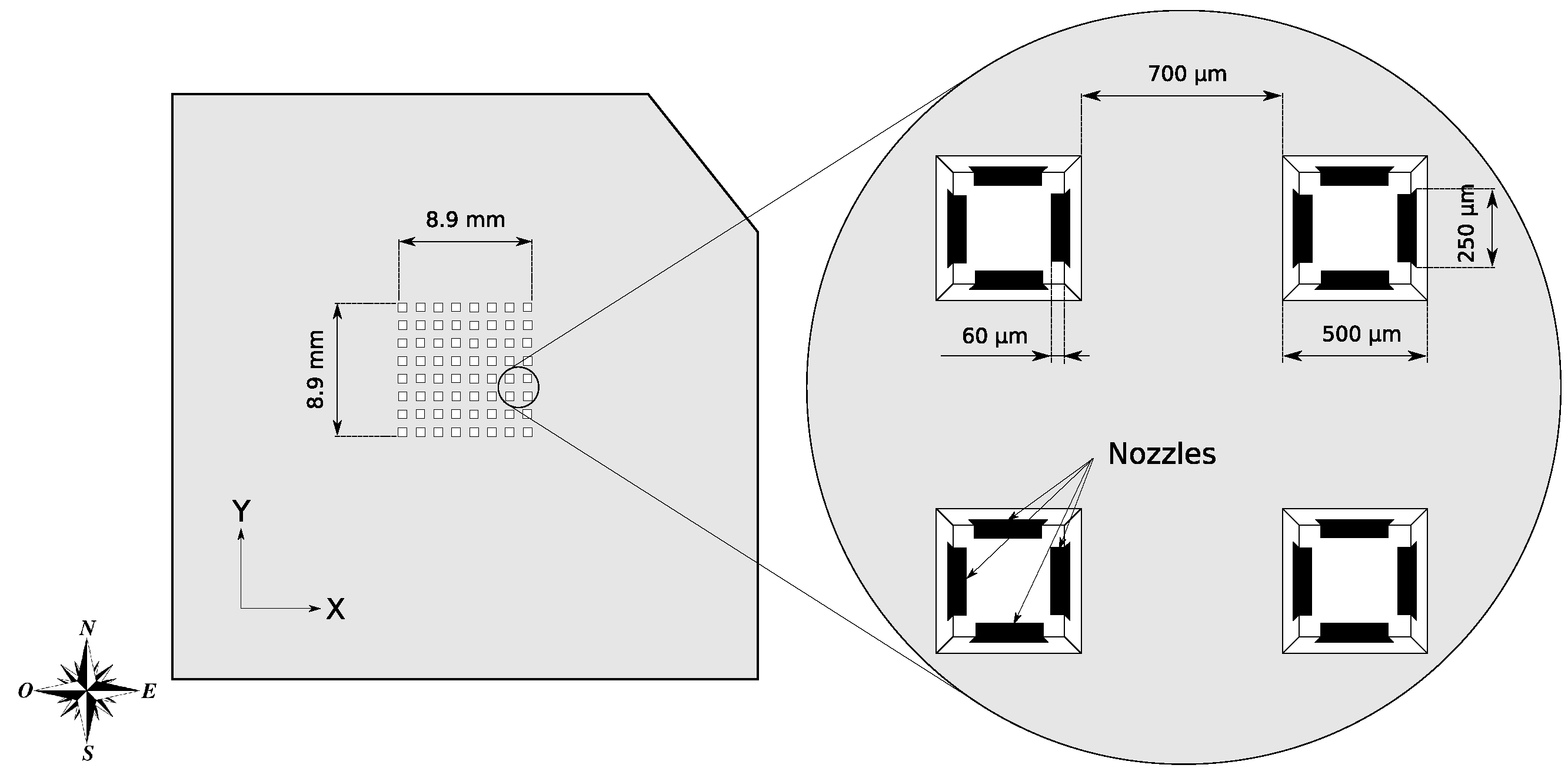
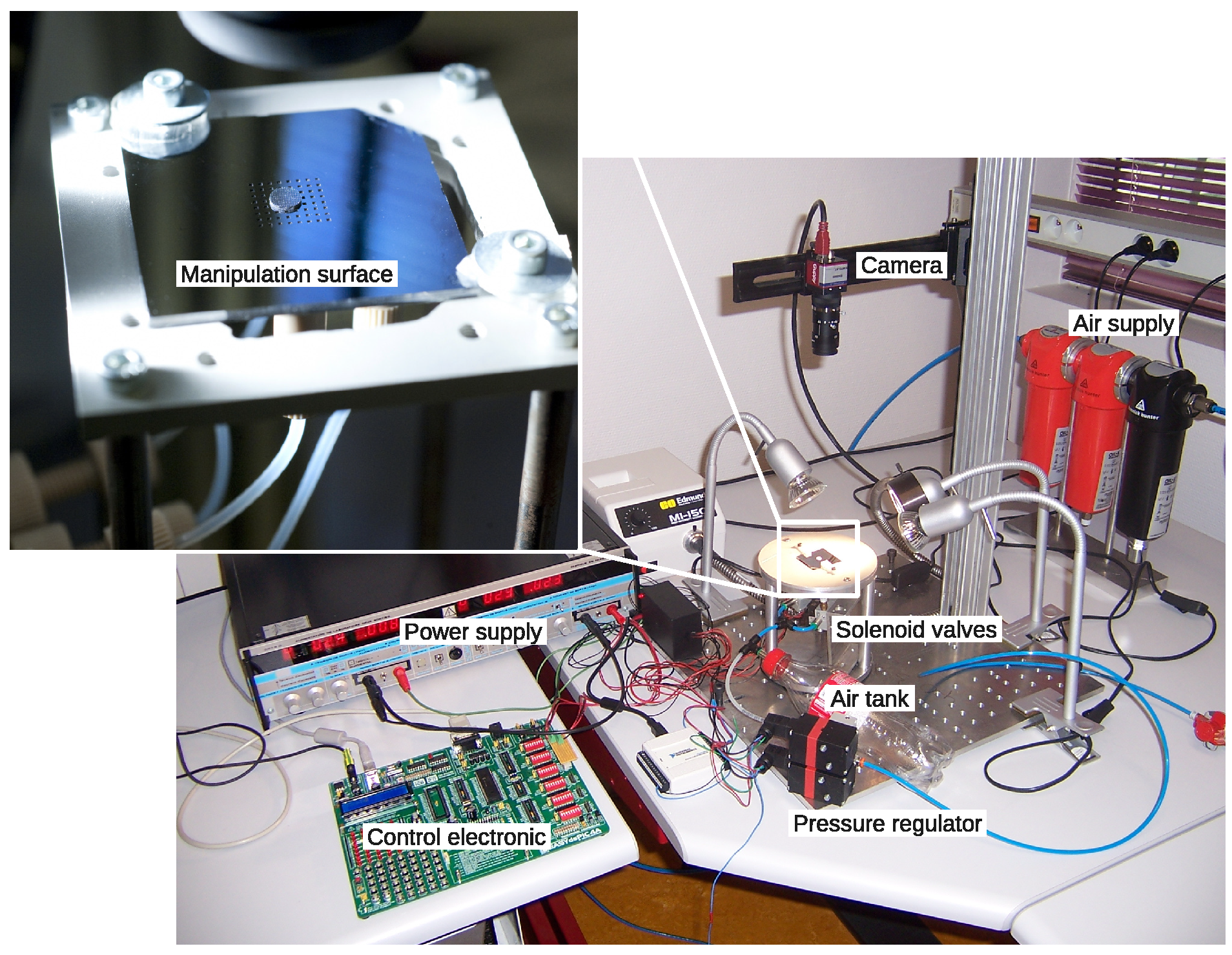
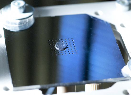
12]. The micro-conveyor consists of a stack of three layers, two silicon wafers and a lower Pyrex glass wafer. The top side of the upper silicon wafer represents the manipulation surface and includes an array of 8 × 8 square holes with four nozzles each (cf.
Figure 1). Its bottom side includes 16 micro-channels which supply the south and north nozzles. 16 other micro-channels which supply the east and west nozzles are etched in the bottom side of the middle wafer. The Pyrex wafer is used to seal hermetically the micro-channels of the middle wafer. Four holes machined in the Pyrex allows for connecting the channels to the air source by means of glued industrial connector. The micro-conveyor has been designed to generate an air jet with an angle of 45° from the vertical [
13,
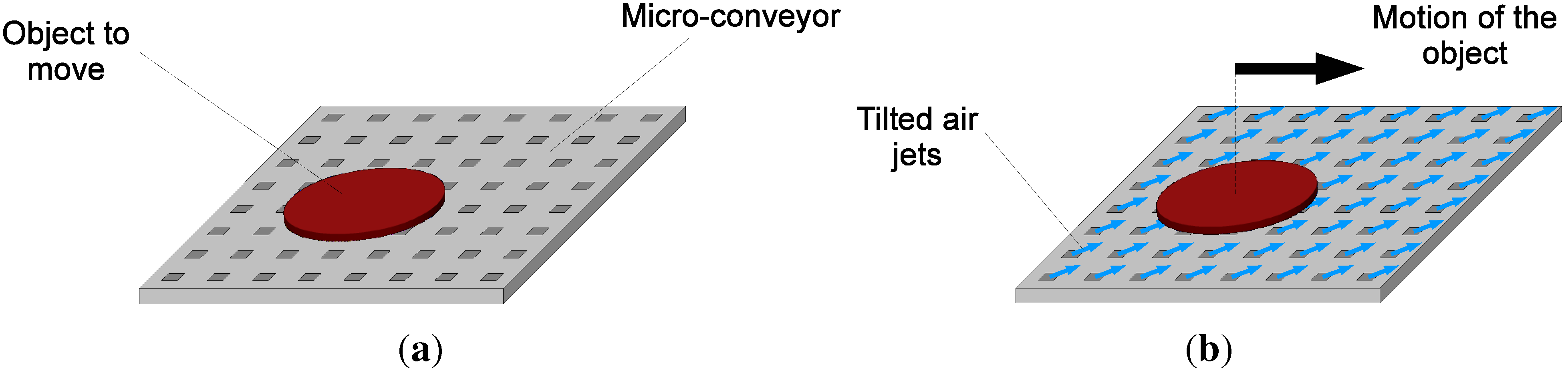
14]. The orientation of the air jets is due to the shift of the holes in the upper wafer. As a result when supplied in one of the four inlets, the micro-conveyor produces an array of 64 tilted air jets that lifts and moves an object in the according direction (cf.
Figure 2) at the same time.
Figure 1.
Top side of the micro-conveyor.
Figure 1.
Top side of the micro-conveyor.
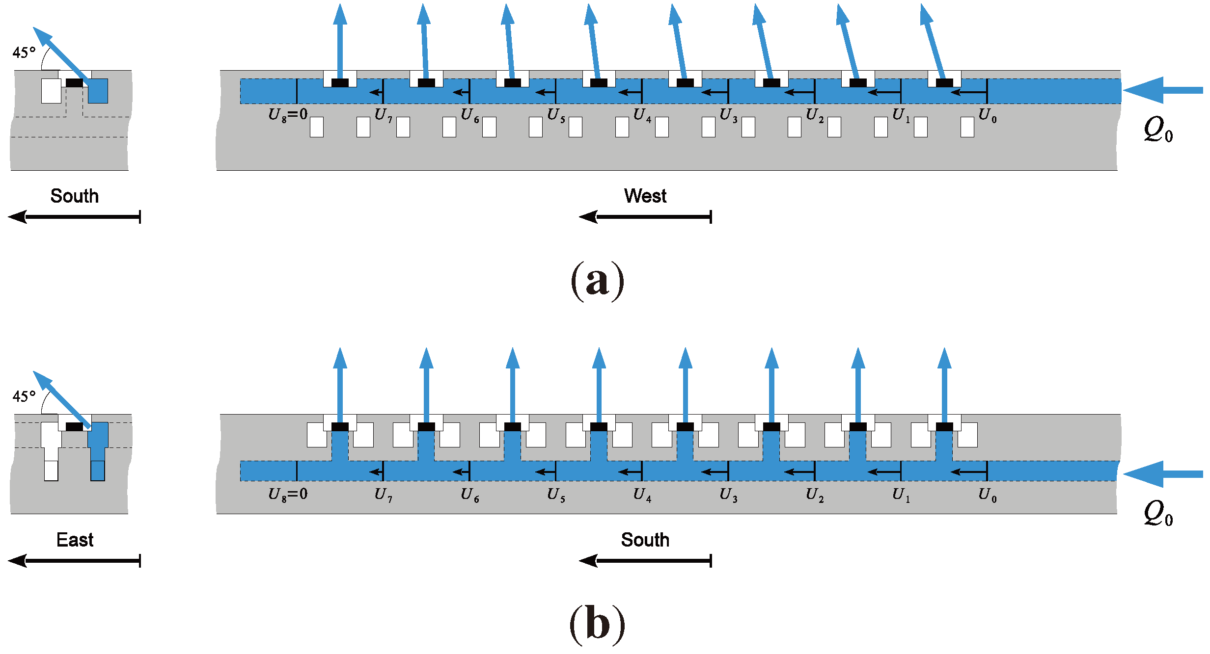
Figure 2.
Working principle of the micro-conveyor. (a) Neutral position (non-blowing); (b) Blowing to the east direction.
Figure 2.
Working principle of the micro-conveyor. (a) Neutral position (non-blowing); (b) Blowing to the east direction.
This micro-conveyor is expected to have several advantages over conventional methods. Using an array of air jets to handle small objects has the advantage of not requiring precision gripping nor a particular contact configuration which may be difficult to obtain for small objects. During the motion, no friction force occurs thanks to the aerodynamic levitation of the object. This may be useful for very fast manipulation.
In this paper, we test the manipulation device and evaluate its performances thanks to the modeling of the dynamics of an object. The next section describes the characterization of the flow. The third part explores the transporting capabilities of the device. The last section presents the experimental determinations of the positioning resolution in open loop and the positioning repeatability in closed loop.
2. Characterization of Flow
Before characterizing the motion of an object over the micro-conveyor, we measured the volumetric flow to determine the head losses in the device and the velocity of the outgoing air.
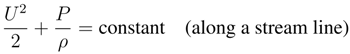
As the used pressures are only several kilopascals near atmosphere, we can consider that the fluid is incompressible. The momentum equation reduces to Bernoulli’s equation. Neglecting the gravity, we have:
where
U and
P are respectively the speed and the pressure at a given point on a streamline,
ρ is the density of the fluid at all points in the fluid.
Considering that the internal fluid is motionless (
Ui = 0) and the relative external pressure is zero (
Pe = 0), this equation gives the exit speed
Ue knowing the internal pressure
Pi before the output nozzle:
Due to head losses, Pi is far below the supply pressure P0. Head loss is divided into two main categories: “major losses” associated with energy loss per length of pipe, and “minor losses” associated with bends, fittings, valves, etc.
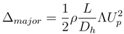
The most common equation used to calculate major head losses is the Darcy-Weisbach equation:
where
Δmajor is the pressure loss due to friction (in Pa),
L is the length of the pipe (in m),
Dh is the hydraulic diameter of the pipe (in m) defined by
![]()
with
s the section of the pipe and
p the perimeter of the pipe,
Up is the average speed of the fluid flow (in m · s
−1) and Λ is a dimensionless coefficient called the Darcy friction factor.
For laminar (slow) flows, it is a consequence of Poiseuille’s law that Λ = 64
/Re, where
Re is the Reynolds number. So, for laminar flows, the major losses are simply defined by:
where
µ is the dynamic viscosity of the fluid (in Pa · s).
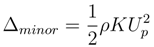
Minor losses are commonly calculated by the following equation:
where
K is a dimensionless coefficient called the head loss coefficient.
To calculate the exit flow according to the supply pressure
P0, we need to write the pressure balance between
Pi and
P0:
Using Equations (2), (4) and (5), we get:
The speed
Up of the fluid flow is equal to the volumetric flow rate
Q per unit cross-sectional area
Sp of the pipe:
In the same, we have
![]()
where
Se is the sum of the section areas of nozzles.
Finally, the volumetric flow rate
Q is the solution of the equation:
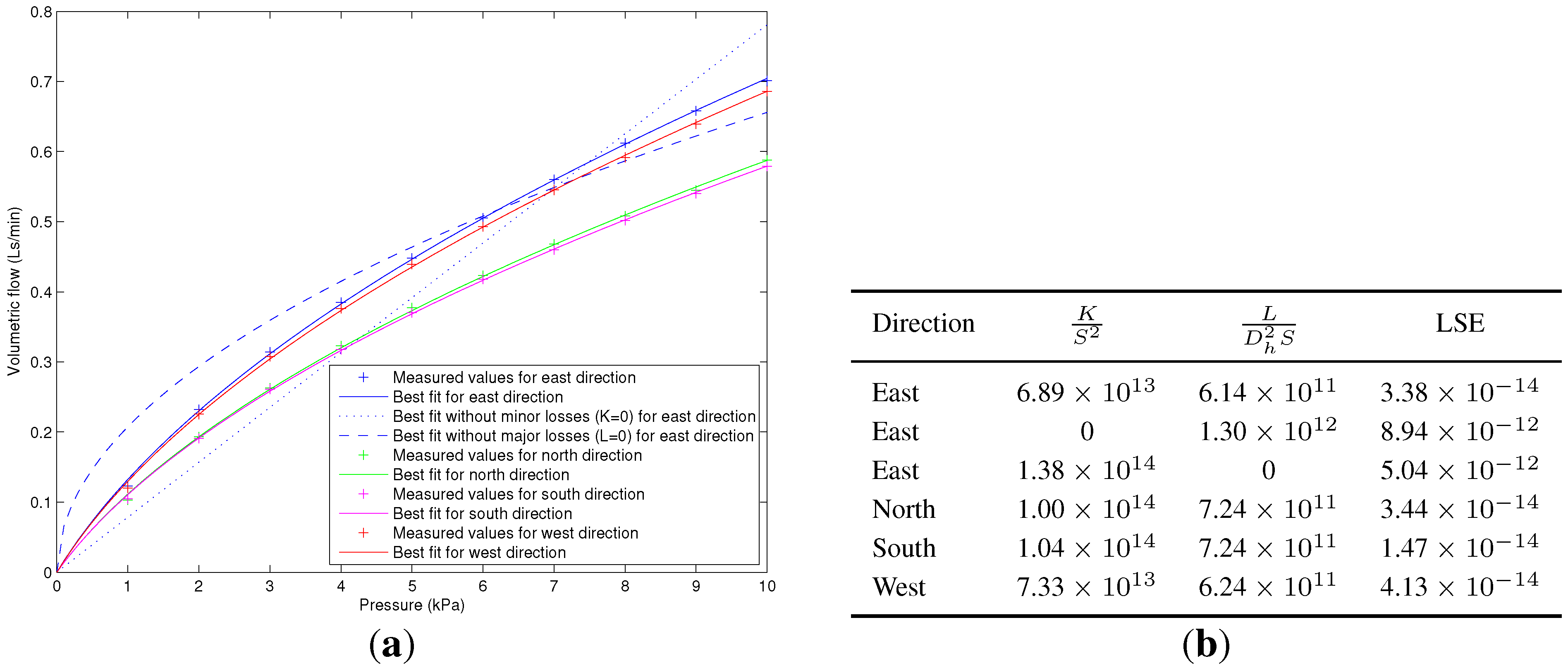
Given this equation and the flow measurements, we can determine the head losses in the micro-conveyor. For 10 values of supply pressure from 1 kPa to 10 kPa, we measured the volumetric flow thanks to a digital flowmeter. Then we calculated the values of losses that minimize the least squares error (LSE) between measurements and theory. The obtained curves and values are presented in
Figure 3. It is noteworthy that if we consider only major losses or minor losses by setting one of the coefficient to zero, the shapes of the curves do not match. If we assume both major and minor losses the theory perfectly matches the measurements. The values of losses are similar in opposite directions. The value of losses are greater for the north-south directions due to the smaller size of channels inside the second layer [
14].
Figure 3.
Least squares fittings for each direction. (a) Flow vs. pressure; (b) Values of minor and major losses.
Figure 3.
Least squares fittings for each direction. (a) Flow vs. pressure; (b) Values of minor and major losses.
4. Positioning Task
In this section, we focus on a positioning task. The aim is to evaluate the device in terms of resolution and repeatability.
4.1. Open-Loop Positioning
First, we tested the response to air pulses. An air pulse is defined by the operating pressure
P0, the duration
Tp of the opening of the valves and the chosen direction (east, west, north, south).
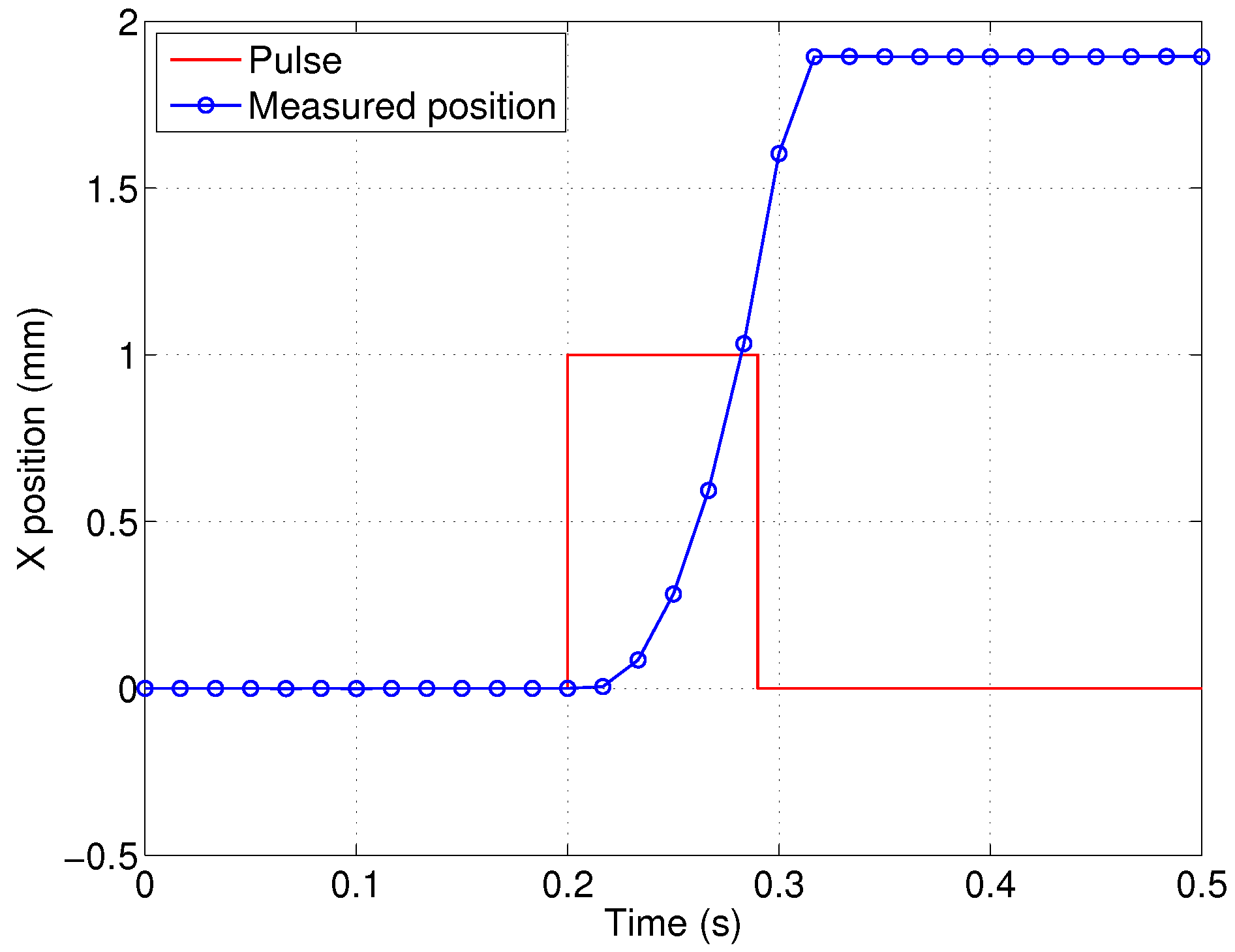
Figure 9 shows the position of the object in the
X direction according to time for a single air pulse toward the east.
Figure 9.
Position of the object according to time for a single air pulse toward the east (mean values on 20 tests). The solenoid valve is supplied when the bold line is equal to one. The pulse width is Tp = 90 ms. The operating pressure is P0 = 10 kPa.
Figure 9.
Position of the object according to time for a single air pulse toward the east (mean values on 20 tests). The solenoid valve is supplied when the bold line is equal to one. The pulse width is Tp = 90 ms. The operating pressure is P0 = 10 kPa.
The response can be described by two different phases: the acceleration and the deceleration. The acceleration phase is identical to the response to a step. The deceleration phase is shorter than the acceleration’s one. This is due to the friction that occurs between the object and the surface when the flow vanishes.
We observed the motion of the object for different pulse durations. The pressure and the initial object position were set to the same values (respectively 10 kPa and the center of the surface).
To evaluate precisely the range of reachable step size, we carried out many experiments with a large range of pulse durations (from 5 ms to 90 ms).
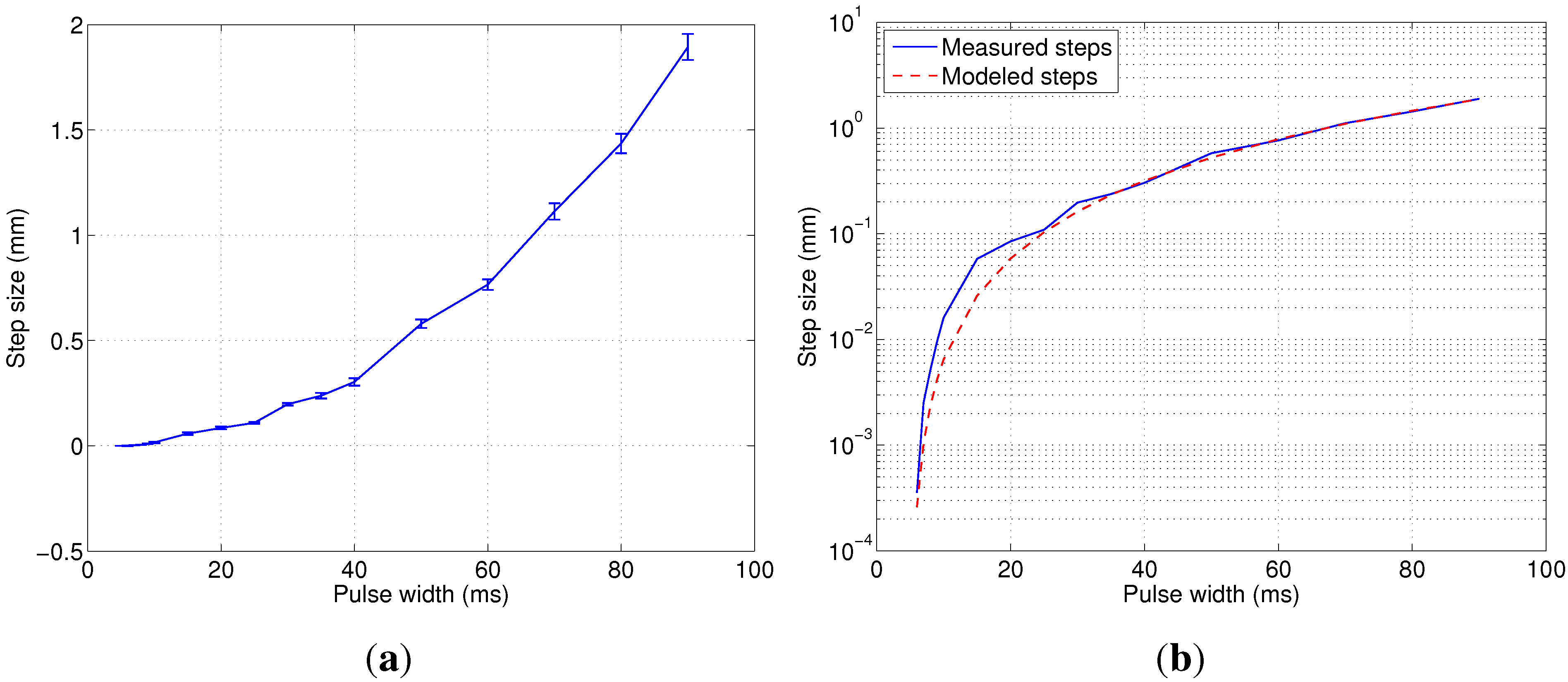
Figure 10 shows the step size according to the duration.
The first thing to note is that the smallest step in the east direction is 0.3 µm. It is surprisingly small for a pneumatic manipulator. In the other directions, the smallest steps are in the same order of magnitude. Actually, as the object is lifted and pushed at the same time, the air cushion removes all dry frictions. Without frictions, there is no stick-slip effect that enables to reach this high resolution.
Figure 10.
Step size toward the east according to the pulse duration (mean values and standard deviations on 20 tests). The operating pressure is P0 = 10 kPa. (a) Linear scale; (b) Semi-logarithm scale.
Figure 10.
Step size toward the east according to the pulse duration (mean values and standard deviations on 20 tests). The operating pressure is P0 = 10 kPa. (a) Linear scale; (b) Semi-logarithm scale.
The second observation is that the step size increases with the square of the pulse duration. The fitted law is given by:
with Δ
east(
Tp) in millimeters and
Tp in milliseconds.
This model is represented by the dashed line in
Figure 10b. Below 5 ms the object does not move at all because the valve does not have enough time to open.
We carried out the same experiments in the three other directions and we obtained similar behaviors:
The last conclusion is that the repeatability of the steps is not so good. We represented the standard deviation on the curve by vertical bars around the points (cf.
Figure 10a). The average relative deviation is around 15% of the length of the step. This poor precision can be explained by the perturbations of the ambient air, by an heterogeneous distribution of the flow and by the motion of the object itself. For example, the pan and tilt angles of the object during the motion are not known. As the number of covered nozzles is not so high, the object may probably tilt during the motion and does not move flat. Different orientations can lead to different forces and then to different step sizes. For these reasons, it is not possible to position precisely the object using only open-loop control. To move the object exactly where we want, we need to measure the current position of the object and to apply a feedback control in order to reduce the position error.
4.2. Closed-Loop Position Control
The aim is to move the object at the center of the surface from arbitrary positions. The desired position (center) is noted (
xref,
yref). Thanks to the camera, the current position of the object is measured; it is noted (
x, y). The position error is given by:
According to the error between the measured position and the desired one, the valve is opened in order to carry the object to the desired position. For instance, if the object is localized at the north of the reference position, a south pulse is generated; if the object is localized at the east, a west pulse is generated; etc.
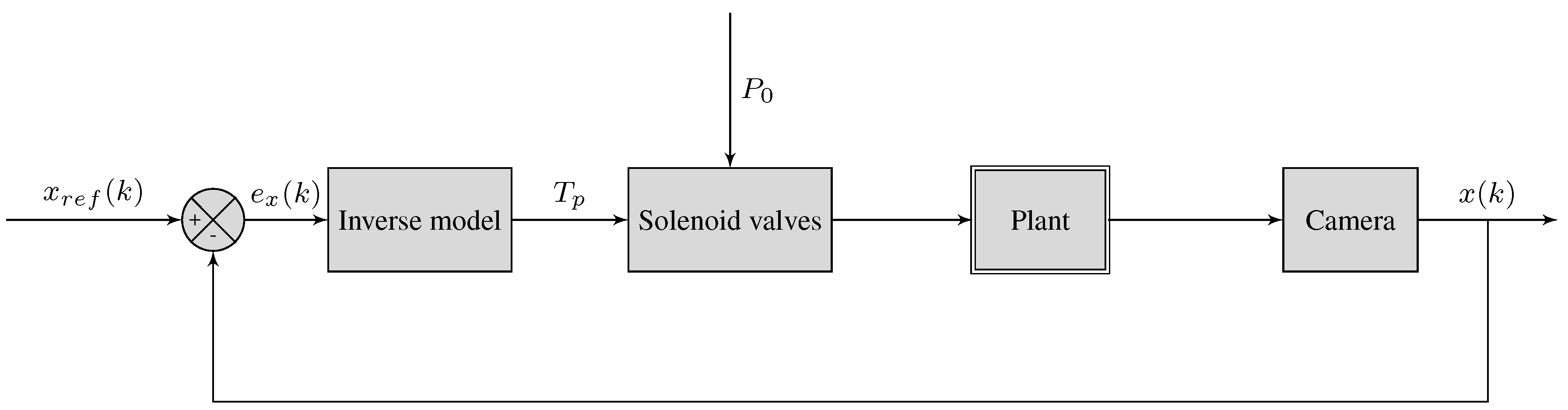
As the aim is to get the highest accuracy, we chose to modulate the width of the pulses as a function of the distance of the object to the target. Thanks to the previous measures, we can deduce the step size from the duration (direct model). So we can calculate the duration in order to get a step size corresponding to the position error (inverse model).
Figure 11 details the feedback loop.
Figure 11.
Feedback loop to control the abscissa of the object.
Figure 11.
Feedback loop to control the abscissa of the object.
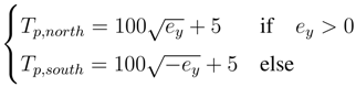
The inversion of Equations (14) and (15) gives for the X direction:
where
Tp,east,
Tp,west are the durations of the pulse corresponding to the east and west directions.
Similar laws can be written for the Y direction:
We performed 20 trials from random positions to evaluate the positioning repeatability following ISO standard 9283 [
18]. The positioning repeatability is defined by,
lj is the distance of the
jth measure to the barycentre,
where
x and
y are the coordinates of the barycentre defined by
![]()
and
![]()
,
l is the mean distance to the barycentre defined by
![]()
.
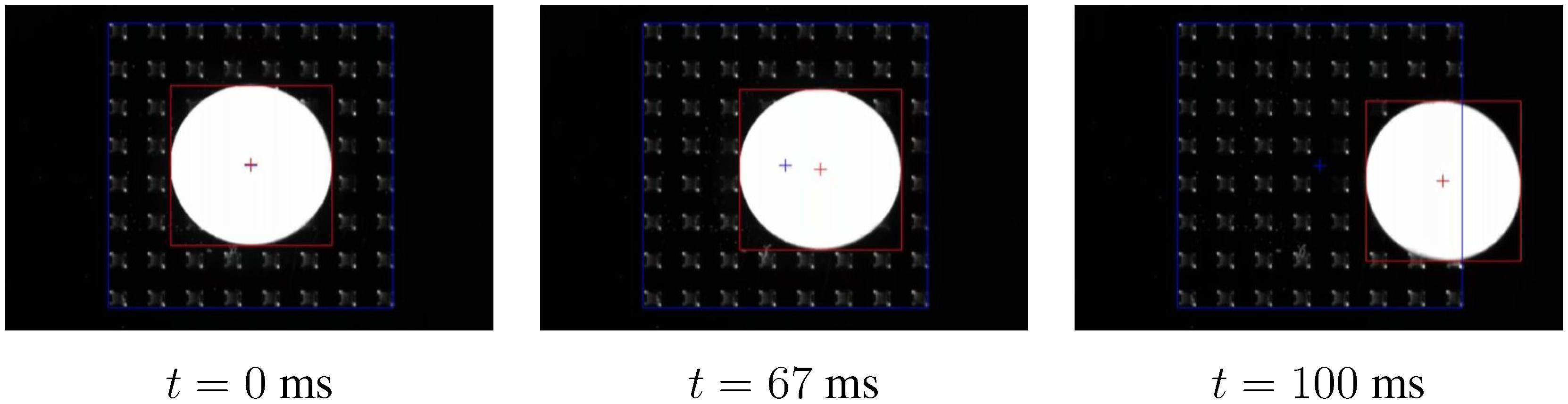
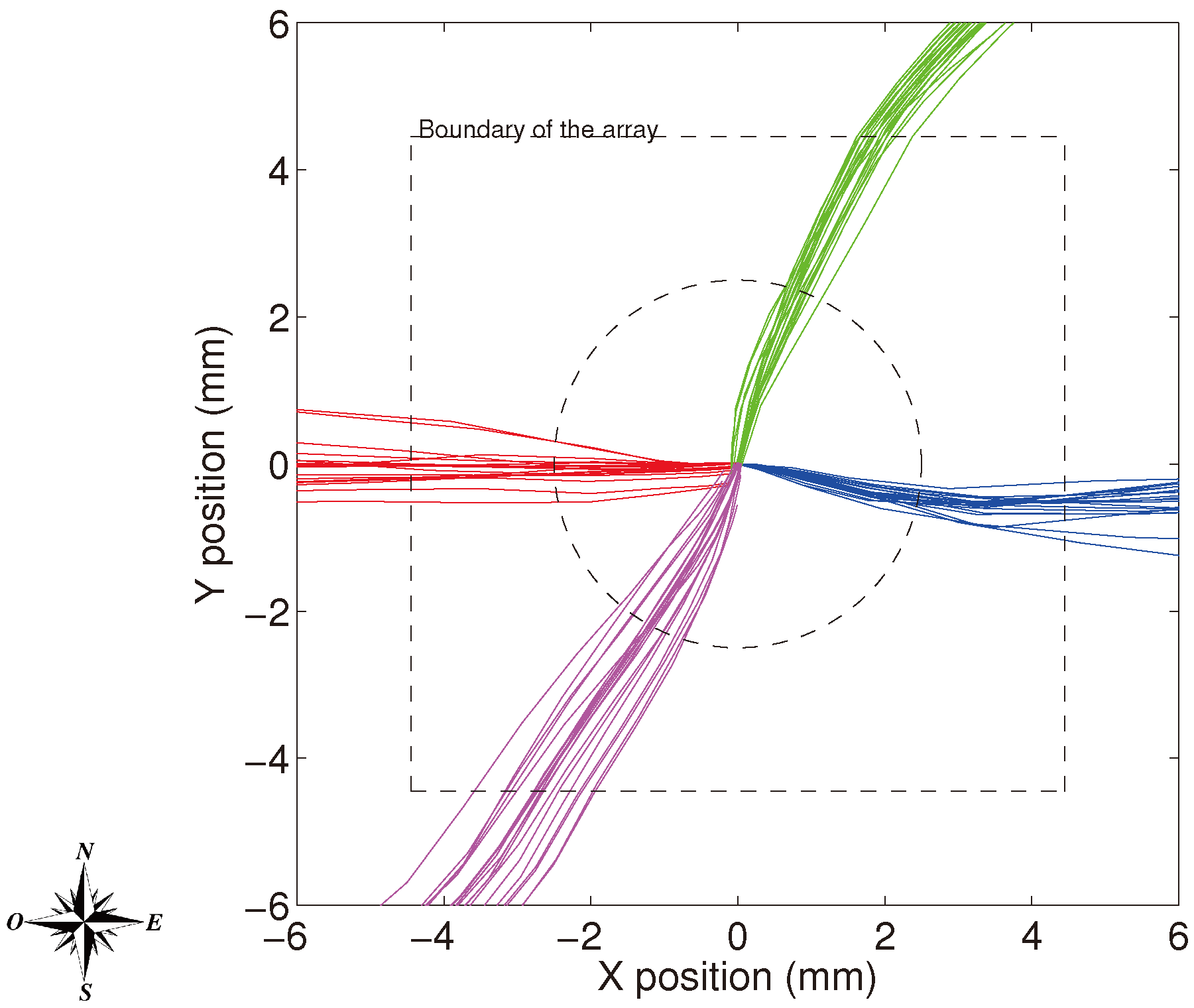
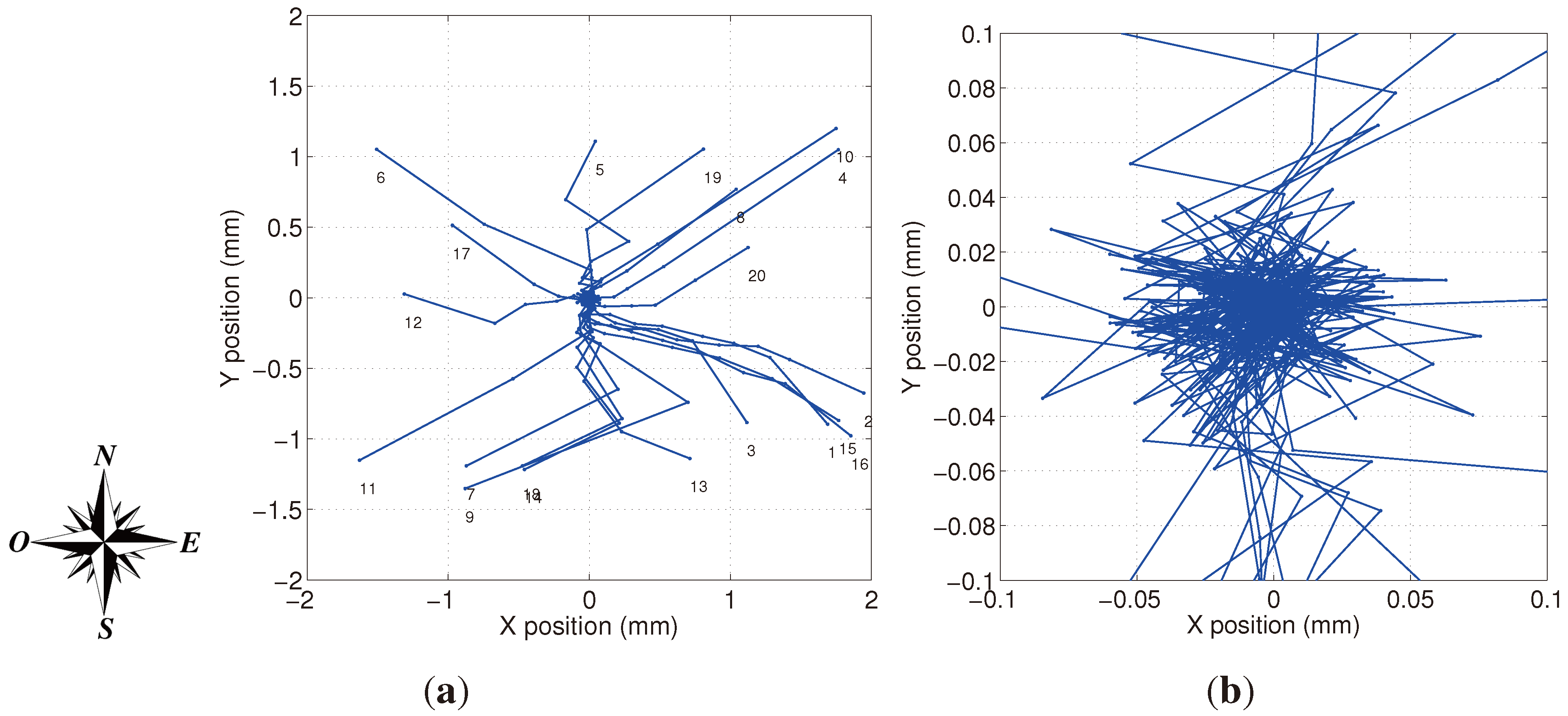
Figure 12 shows the trajectory of the object for each test. These experiments can be further appreciated in the video clip accompanying this paper. The positioning repeatability is 17.7 µm. This value is a lower bound of the accuracy we could obtain with the proposed feedback control.
Figure 12.
Path of object from 20 arbitrary positions to the center of the surface with the feedback controller. (a) Large view; (b) close view.
Figure 12.
Path of object from 20 arbitrary positions to the center of the surface with the feedback controller. (a) Large view; (b) close view.
The object needs five steps on average to reach the final position. We could think that only one step is necessary since we used the inverse model to calculate the pulse width. The first explanation is the poor repeatability of the size of the step for a given pulse duration. The second one is that the model has been established in the center of the surface and performances are lower near the edges of the surface. So the first step is often shorter than expected as we can see in
Figure 12. The last reason is that we did not take care of coupling. So when the object is near the center and for example both west and south directions are activated the amount of air is too high and the object overshoots the mark. Future works on the control could reduce the number of steps and maybe improve the positioning repeatability.
5. Conclusions
In this paper, we tested a micro-conveyor able to produce an array of tilted air jets. The performances are summed up in
Table 2. It is noteworthy that this device is able to move the object with high speed relatively to its size and also to position it with a good precision. For instance, the object can reach a speed of up to 137 mm · s
−1 in open loop whereas the positioning repeatability is around 5 µm with closed loop control. The smallest step the object can do is 0.3 µm (resolution). Moreover, we estimate that the speed could reach 456 mm · s
−1 if several micro-conveyors were used to form a conveying line.
Table 2.
Performances of the micro-conveyor.
Table 2.
Performances of the micro-conveyor.
| Size of manipulated objects | 1 mm to 10 mm |
| Maximal speed on one micro-conveyor | 137 mm · s−1 |
| Estimated maximal speed on a line of micro-conveyors | 456 mm · s−1 |
| Resolution (smallest step) | 0.3 µm |
| Positioning repeatability (ISO 9283) | 17.7 µm |
| Maximal air consumption | 1.83 ls/min |
Compared to existing devices, the micro-conveyor outperforms them in terms of speed and precision. Concerning the bandwidth, the device is in the middle range. During the experiments, we saw that the object reaches its maximal speed in about 100 ms before leaving the array. This settling time included the opening of the valve, the establishment of the flow and the behavior of the object in the flow. It could be improved in the future by using faster valves and shorter pipes.
Another advantage of the device is its sturdiness since a movable part does not exist inside the wafers. The valves require only conventional technologies that are cheap and robust.
Considering industrial applications, the upper space is free and enables the access for a robot to pick or place objects on the surface. We carried out some experiments with different kinds of objects which can be seen in the video clip accompanying this paper. The micro-conveyor can move cylindrical objects from 1 mm to 10 mm, but also various objects as electronic parts if the backside of the object is flat. In the future, we can imagine building large conveyor systems able to carry small parts at high speeds and to position them with a good accuracy when required.

 ,
, 


 with s the section of the pipe and p the perimeter of the pipe, Up is the average speed of the fluid flow (in m · s−1) and Λ is a dimensionless coefficient called the Darcy friction factor.


 where Se is the sum of the section areas of nozzles.


 and
and  , l is the mean distance to the barycentre defined by
  .
.