2. Mathematical Modeling
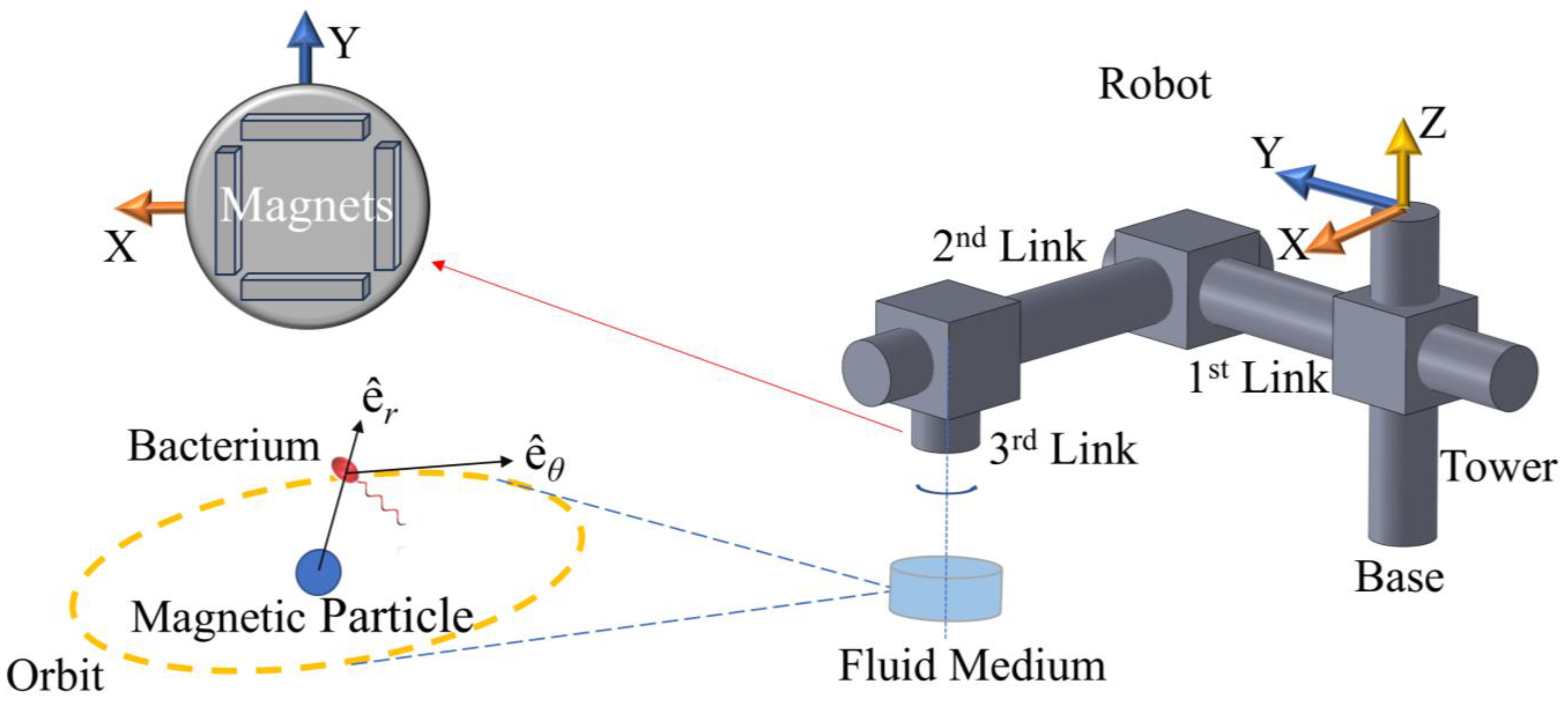
The physical setup to be modeled is comprised of a robotic arm, four magnets, micro-tweezers, and a bacterium cell.
Figure 1 depicts this system as simulated in this study. The hydrodynamic tweezer system is comprised of a spherical magnetic particle, 100 μm in diameter, submerged in water at room temperature revolves under the influence of a rotating magnetic field of four permanent magnets of type-N52 Neodymium [
26]. The overall density of the spherical particle is assumed to be balanced out by the magnetic pull in the direction of gravitational pull; therefore, it is assumed to be just beneath the surface avoiding sedimentation at the bottom, by design. The rotation rate and the displacement of the magnetic field are controlled by a prismatic-prismatic-revolute joint robotic arm (please see
Table 1) articulated by three dedicated DC motors at the respective joints. The spherical magnetic particle is rotated and dragged by the external magnetic field, which generates the vortex in question to help manipulate the selected bacterium, i.e., an
E. coli minicell [
25]. The magnets are located at the edges of a square of the same length. The revolute joint, i.e., the said arrangement of magnets, and the micro-tweezers, i.e., the spherical magnetic particle, are perfectly aligned at
t = 0 s. The alignment is broken once the arm starts following the control signal and the vortex core traverses along XY-plane (see
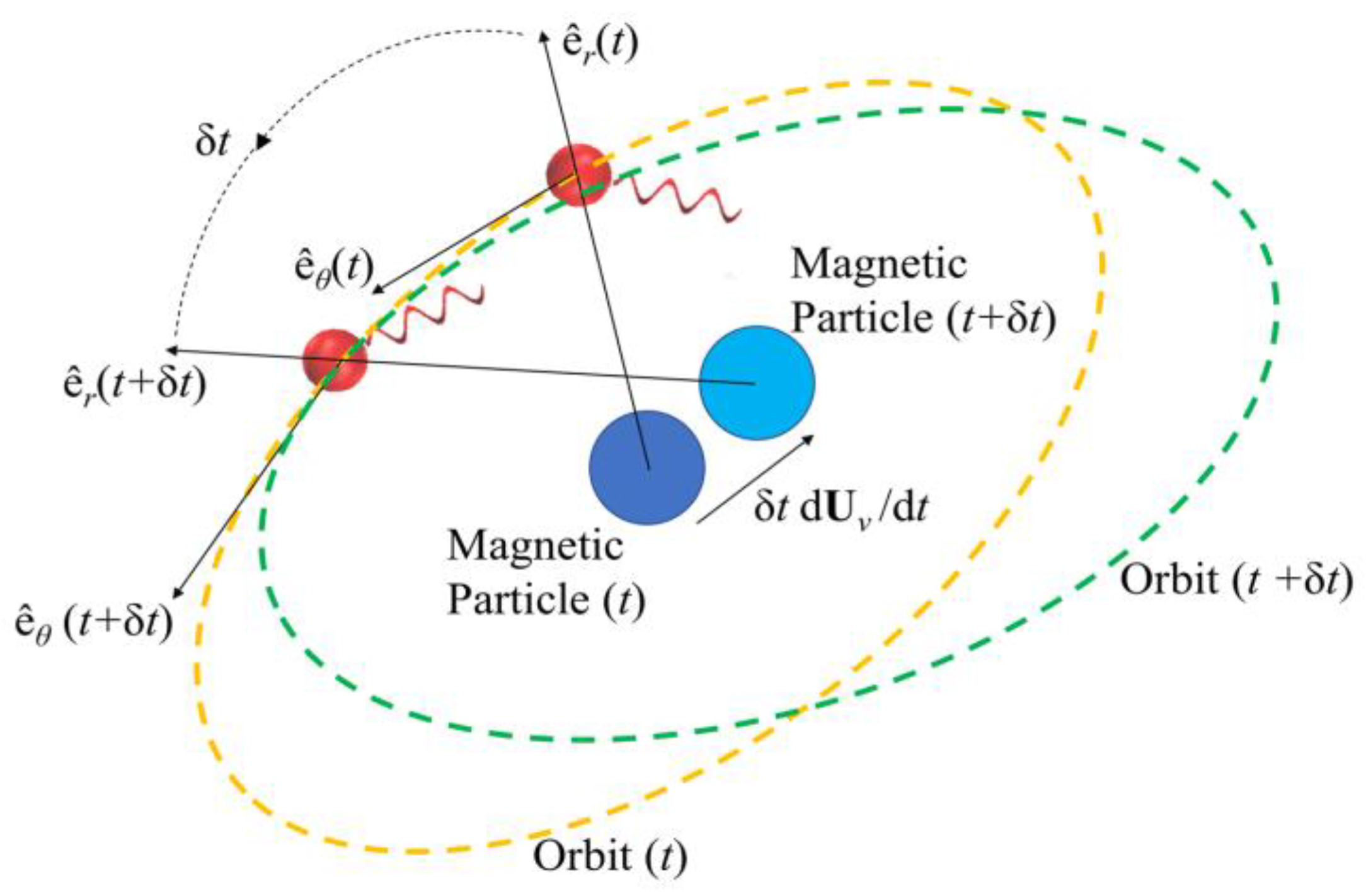
Figure 2). The robotic arm is expected to stay ahead, whereas the vortex is expected to lag. Furthermore, the
E. coli minicell is assumed to be unmodified and possessing no magnetic properties, and thus, it is not going to be directly affected by the magnetic fields as magneto-tactic bacteria, such as Magnetospirillum
Gryphiswaldense [
27] or a modified
E. coli [
28], reported in the literature, would have reacted.
Figure 2 depicts the hydrodynamic tweezers moving along the XY-plane as the
E. coli minicell orbiting its core. The resultant orbit is a transient gait that evolves along with the rigid-body motion of the vortex core. As the magnetic particle moves under the influence of the external magnetic field, the bacterium experiences a transition from the orbit at the instant “
t” to the new orbit at the instant of “
t + Δ
t”. This is only possible if the bacterium is trapped by the forced vortex: the induced pressure difference of the circulation pushes the bacterium in the negative radial direction, i.e., towards the vortex core. Meanwhile, the circulating flow field drags the bacterium in a curvilinear path. The bacterium can propel itself in any random direction, but the thrust force of the rotating tail is not comparable enough to escape from this trap. In return, the bacterium is forced to follow the vortex core as the invoked rigid-body rotation of the spherical magnetic particle drives the flow and pressure fields, while inertial forces do not dominate the overall dynamics for the bacterium cell. The two-way coupled equations of motion for the bacterium cell and the vortex core govern the overall interaction between the two while predicting the velocity field with the associated pressure and drag force profiles. The following detailed model further explains how this interaction occurs.
The rigid-body motion of the bacterium is a cumulative result of propulsion and drag. It is the rotation of the helical tail and body in opposite directions along with the simultaneous hydrodynamic and the tactile interactions with the forced vortex that govern the acceleration. The interaction between the bacterium and the spherical magnetic particle at the center is somewhat complex. The phenomenon could be explained by studying the elements separately by assuming Stokesian flow dynamics and elastic collisions [
14,
29]; however, the problem is complicated given that all of these effects are inevitably coupled as all depend on the instantaneous position of the bacterium with respect to the spherical magnetic particle.
The equation of motion (1) for the bacterium is given as follows:
governing the six-degrees-of-freedom (6-dof) motion in the inertial frame of the vortex with the rigid-body traverse of
Ub = [
ur uθ uz]
T and rigid-body rotation of d
Θb/d
t = [
ωr ωθ ωz]
T. It should be donated that these two vectors arise due to the circulating flow field only. The core of the matrix moves, and the bacterium realigns itself under the influence of the pressure force and azimuth drag. This behavior is independent of its own propulsive behavior. The propulsive effect of the bacterium tail in the equation above is denoted by
Fp, i.e., the force vector with the subscript “
p”, respectively. These are calculated based on the resistive-force theory that has been studied extensively [
30,
31]. It should be noted that the propulsive effect is also dependent on the proximity of the bacterium and the vortex core [
32]. The rest of Equation (1) can be listed as follows: (i) the viscous drag vector acting on the bacterium cell due to its own motion following the propulsion of the rotating helical tail,
Fd; (ii) the vector of drag and pressure forces purely induced by the vortex itself [
14,
29],
Fv; (iii) the contact force when an elastic collision occurs [
14,
29],
Fc; (iv) the dampening effect due to lubrication and film damping of the fluid film exhibited with proximity [
14,
29],
Flub+fd; and (v) the effect of added mass on the azimuth direction where the material derivative can be approximated effortlessly [
33],
Fadd. Similarly, the torque components can be defined as (i) the propulsive torque of the rotation tail [
30,
31],
Tp; (ii) the pure drag of rigid-body rotation, [
30,
31],
Td; (iii) the torque due to lubrication and film-damping effects [
14,
29],
Tlub+fd; and (iv) the shear torque on the bacterium body due to asymmetries of the flow field along the radial and vertical directions [
14,
29],
Ts. Here,
Ts should be projected on the inertial frame of the vortex from the bacterium frame via an associated instantaneous rotation matrix,
Rb→v, for it is originally calculated in the inertial frame of the bacterium cell. The terms on the left-hand side are diagonal mass,
mb, and moment of inertia,
jb, matrices associated with the bacterium.
If one is to investigate these components in more depth in the respective order, the equation
represents the propulsion force with the help of the three-by-six translation-resistance matrix,
Gtail, of the rotating helical tail of the bacterium along with its reported rotation rate,
ωtail, harnessing the necessary thrust force [
25,
30,
31]. The
0 on the right-hand side denotes a three-by-one vector with all elements being equal to zero. Also,
,
, and
denote the unit vectors in the inertial frame of the forced vortex, respectively. The ensuing hydrodynamic drag to the overall rigid-body motion of the body of the bacterium cell is given by
with
,
, and
denote the effective drag coefficients pertaining radial, azimuth, and perpendicular directions [
34,
35], respectively.
Next, the force vector comprising radial pressure and azimuthal drag, associated with the presence of a nearby forced vortex as discussed before, is predicted as follows:
Here, in Equation (4),
a denotes the radius of the body of the
E. coli Minicell [
25];
ρ denotes the density of the liquid medium, i.e., water at room temperature;
rb(
t) is the radial distance of the bacterium cell to the vortex center;
Ωz is the rotation rate of the spherical magnetic particle;
R is the radius of the spherical magnetic particle; and
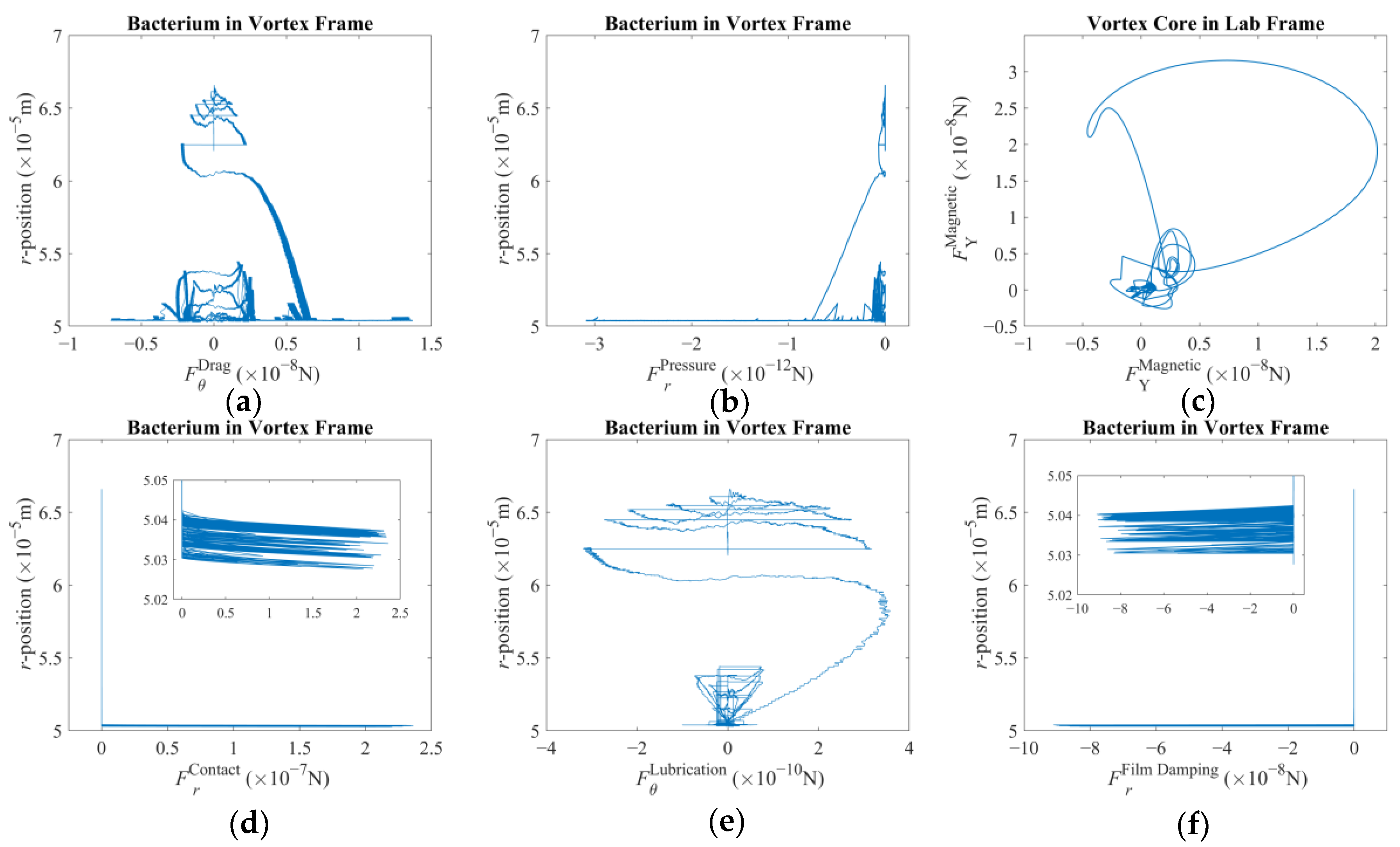
r stands for the radial position in the vortex frame over which the integral is taken. Here, it is assumed that there is no considerable force along the z-direction; thus, zero denotes no contribution in the respective direction. This vector equation yields negative pressure force regardless of the direction of the vortex rotation, thereby pushing the trapped particle always in the negative radial direction. On the other hand, the azimuth component is observed to be in favor of the direction of rotation. Once the vortex core is incrementally displaced, these force components will be affected but in magnitude alone. The trapped particle will again be compelled to follow a similar path. It can be argued that the rest of the interaction effects arise secondary to the
Fv vector as described here.
The contact force is given with a simple condition in part on the direction of motion expressed as follows:
with
c,
δr, and
b being the stiffness coefficient, penetration depth, and damping coefficient at the point of contact with the magnetic particle [
14,
29], respectively. Surfaces can further be tailored to repel cells [
36], leading to customized contact coefficients. Here, the coefficients are set to simulate repulsion upon tactile contact. But, before the tactile contact occurs, an additional hydrodynamic interaction takes place that can be modeled as follows:
with
μ,
h, and
giving the dynamic viscosity of water at room temperature, the distance along the common normal of the bacterium and spherical magnetic particle surfaces, and the relative azimuth-velocity between the surfaces at proximity [
29,
37,
38] respectively. A lubrication effect is felt along the azimuth, whereas the film damping is felt in the radial direction, prior to contact.
The added mass effect on the bacterium cell is incorporated with the inclusion of the material derivative, D/D
t, as follows:
assuming that the main component of the motion in the vortex frame will be along the direction of the azimuth [
33]. Here,
is the reported volume of the bacterium cell [
25].
The torque components in Equation (1) are given similarly as follows:
with
Etail being the three-by-six matrix of rotation-resistance in the vortex frame [
30].
Furthermore,
gives the torque acting on the bacterium cell due to rigid-body rotation with
,
, and
denoting the effective rotational drag coefficients pertaining radial, azimuth, and perpendicular directions [
34,
35], respectively, in the vortex frame akin to Equation (3).
The torque induced by lubrication and film-damping is modeled with the help of a simple cross-product given as follows:
The final torque component acting on the bacterium arises due to asymmetries in the flow field of the forced vortex and modeled as follows [
29]:
Here,
zb(
t) is the instantaneous position of the bacterium along the vertical axis [
29]. The said asymmetries arise due to unequal radial and vertical distance between arbitrary points on the spherical surfaces of the magnetic particle and the bacterium body that result in additional rotation in return.
Once the equation of motion and respective frames are established for the bacterium cell, the next step is to articulate the equation of motion for the spherical magnetic particle in the same fluid medium. The most important stimuli to account for are the magnetic field and the drag of the experienced relative flow field due to its own rigid-body motion. The other forces exerted on the core of the vortex can be omitted based on a sole inertia comparison in between the spherical magnetic particle and the bacterium cell. However, lubrication force is included given the low-Reynolds-number flow condition. Therefore, the equation of motion preferred in this study is given as follows:
for 6-dof motion in the inertial frame of the vortex due to the rate of rigid-body traverse, i.e.,
Umag = [
v x v y v z]
T, and the rate of rigid-body rotation, i.e.,
Ωmag = [
Ω x Ω y Ω z]
T, [
14,
29]. It should be noted that additional interaction effects shall be included should the size and inertia of the two particles become comparable.
The magnetic force vector acting on the vortex core is given as follows:
with rotation matrix,
Rr→v, to project the gradient of the magnetic field,
B, from the frame of the robotic arm to the frame of the forced vortex. Here,
, is the volume of the spherical magnetic particle. The term
Mp is the instantaneous total magnetization vector of the particle in question and allows one to calculate the magnetic stimuli at any given instant, in the following form:
with
T,
k,
m, and
γ denote the absolute temperature of the fluid, Boltzmann constant, magnetization value for a single super paramagnetic iron oxide nano particle, and number density of the particles in the spherical magnetic object [
39,
40,
41,
42], respectively. Here, the number density is found via the mass fraction of the nano particles mixed with resin along with the neutral buoyancy assumption, assuming the bulk resin density is around 700 kg/m
3. Also, L is the Langevin function [
41] representing the magnetization profile of the nano particles. The magnetic field is in fact calculated as the linearly superimposed magnetic fields of four separate permanent magnets placed in a square formation, i.e.,
B = [Σ
Bx Σ
By Σ
Bz]
T, expressed in the frame of the end-effector of the robotic arm [
43] yielding symmetry along the
Z-axis of the respective degrees of freedom. Furthermore, each magnetic field component is expressed as a combination of three intricate spatial functions, G
(1,2,3), so that the field vector and its gradient can be properly calculated [
44]:
where
is the magnetization of the selected material, i.e., type-N52 Neodymium [
26] for this study. Furthermore,
μ0 denotes the permeability of empty space, while
xrel,
yrel, and
zrel signifing the relative position of the magnetic spherical particle with respect to each magnet, respectively.
The fluid drag on the spherical magnetic particle is given by the following:
The torque components in Equation (12) are also presented by the following:
and
Equations (1)–(18) are used for the deterministic prediction of rigid-body accelerations. However, it is known that there will be stochastic displacement of the bacterium cell due to Brownian noise [
35]. A simple approach to include such an effect is arguably to superimpose this random motion and the deterministic calculations of rigid body motion, i.e.,
db(
t) = [
rb (
t)
rb (
t)
θb (
t)
zb (
t)]
T and
Θb(
t) = [
θX (
t)
θY (
t)
θZ (
t)]
T, as follows [
35]:
Here, each separate term
{r, θ, z, rr, θθ, zz} used in Equations (20) and (22) denotes a random selection of ±1 with uniform distribution over time for the respective degree-of-freedom such that the jumps will take place in random directions along all axes. Moreover, δ
t stands for the duration of the spatial and rotational jumps, i.e., the time-steps taken by the ODE solver. Therefore, the resultant position and orientation of the bacterium cell at the end of each time step, i.e., r
∑(
t + δ
t) and Ψ
∑(
t + δ
t), are employed in the equations of motion for the calculation of the next iteration. It is important to acknowledge that Ψ
∑(
t + δ
t) is presented in terms of Euler angles [
43].
Finally, we have the equations for the robotic arm of three-degrees-of-freedom with the Denavit–Hartenberg parameters provided by
Table 1. The selection of the parameters drastically simplifies the inverse kinematics [
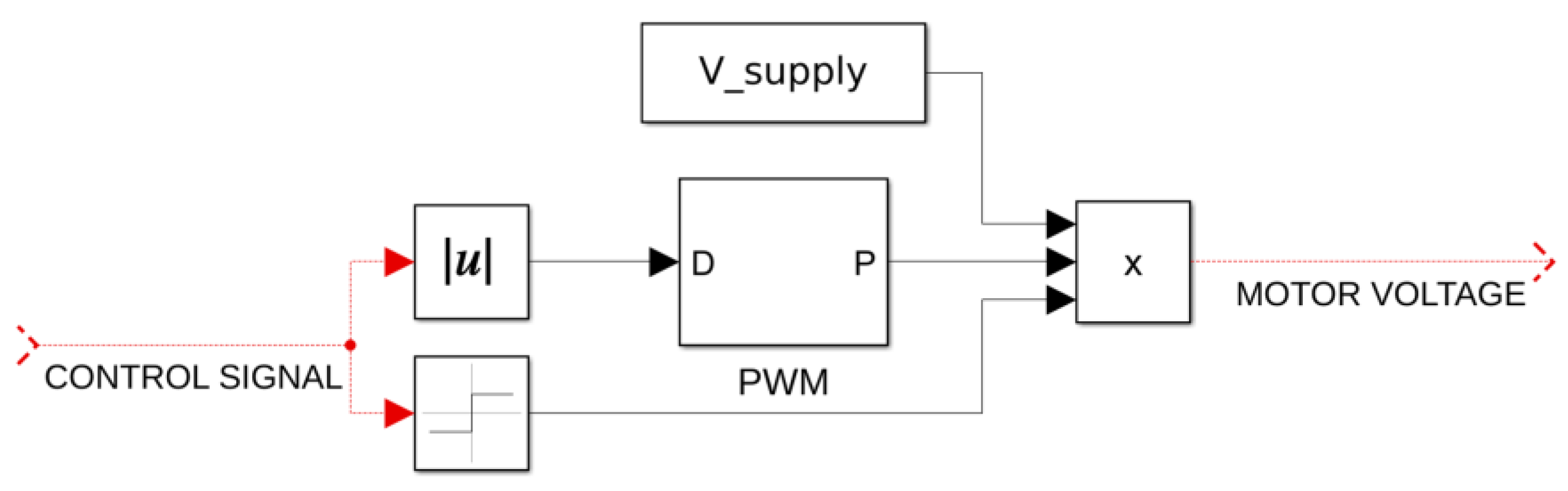
43]. Each degree of freedom is articulated by its own dedicated DC-motor of the same type, i.e., EC 45 Flat brushless 48 V & 70 W (Maxon Group). The respective equations representing the dynamics of the robotic arm and the DC motors at the joints are as follows:
In
Table 1, the twist angles,
α{tower,1,2,3}, represent the x-rotation of each link with respect to the previous joint; the lengths
l{tower,1,2,3} represent the distance between two consecutive joints residing on the same link and along the
X-axis associated with the latter; offsets
d{tower,1,2,3} represent the distance between two consecutive joints residing on the same link and along the
Z-axis associated with the latter; and the rotations
θ{tower,1,2,3} denote the rotation between two consecutive joints residing on the same link and along the
Z-axis associated with the latter. Now, it should be acknowledged that, at the end of the third link, there are four permanent magnets constituting the end-effector with no additional geometric features to account for. Also, the tower in
Table 1 serves as an initial offset to initially position the magnets over the fluidic medium, only.
Above, in Equation (23), the terms
Darm,
qarm,
Kmotor, and
Imotor give the effective diagonal inertia matrix for the robotic arm owing to the prismatic–prismatic–revolute joint arrangement as presented in
Figure 1 and
Table 1, the generalized coordinates for the robotic arm, i.e., the open-kinematic chain as
qarm = [X Y
θZ ]
T, the diagonal torque constant matrix, and the motor current vector, respectively [
43]. Here,
θZ denotes the rigid-body rotation of the third link with the permanent magnets depicted in
Figure 1. Also, we use the following equation of
with
Lmotor,
Rmotor,
Vmotor, and
Kemf signifying the diagonal inductance matrix, armature current vector, diagonal resistance matrix, motor voltage vector, and diagonal friction coefficient matrix, respectively. This last matrix equation brings all the electromechanical properties associated with the three DC motors used at the joints together [
43].
Finally, having the entire dynamics expressed in this form leads to the control law summoned in this study. As discussed before, once a position reference is provided, the end-effector is expected to traverse the magnetic field and the micro-tweezers are expected to follow with a variable reaction time, mostly owing to the viscous drag accompanied by the magnetic response of the super paramagnetic nanoparticles. Therefore, a novel approach was investigated with a weighted control signal of two distinct tracking errors: both being used for proportional and integral (PI) control. Furthermore, the integral control is of an adaptive nature [
45,
46] to tune the output according to the error. The control law and the control signal,
η, pertinent to the X- and Y-axes, i.e., the laboratory frame, used for this study are as follows:
with
fR and
fV indicating the tracking error for the end-effector of the robot and the spherical magnetic particle, respectively. Therefore, the controller is incorporating two distinct velocity and position informations. The proportional and integral gains are denoted by
kp and
ki, respectively. The formulation of the integral control is of an adaptive nature, whereas the proportional gain is constant [
43,
45,
46]. It is also noted that only one set of PI-control gains is used for these two degrees of freedom. The weighing coefficient
β ensures that the total contribution adds up to unity. The role of the integral gain is to minimize the steady-state error but here, unless
β ≈ 0.5, the control law will either focus on the end-effector or on the vortex core to achieve the best performance. Since there is no tactile contact or tether between the third degree-of-freedom and the spherical magnetic particle, this approach will yield the best performance for one at the expense of the performance of the other. Furthermore, it should be argued that there are three criteria that directly affect the determination of
ki,
kp, and
β: (i) the tracking error that is being minimized, (ii) the reaction time of the overall system, and (iii) the level of misalignment between the vortex core and the third degree-of-freedom. Here, it can be argued that the last criterion is favored at the expense of others.
As opposed to the XY-traverse, the control signal generated for the third degree-of-freedom, i.e., the rotation rate of the magnets, is a simpler P and adaptive-I control as ηz = kpfR−Ω + ∫ 1/((ki fR−Ω)2 + 1) dt, with fR-Ω representing the error between the rotational velocity reference. Here, the calculated error is solely based on the rotation rate of the third degree-of-freedom. It should be noted that detecting the rotation rate of the vortex core might be impractical in real applications; therefore, it is not included in the control law. It should be noted that there are three control inputs but twelve degrees-of-freedom in total, i.e., the first three belonging to the robotic arm, then three more associated with the spherical magnetic particle, and finally six degrees-of-freedom for the untethered swimming of the bacterium cell. Therefore, the model here represents an under-actuated multi-scale robotic system.
4. Discussion
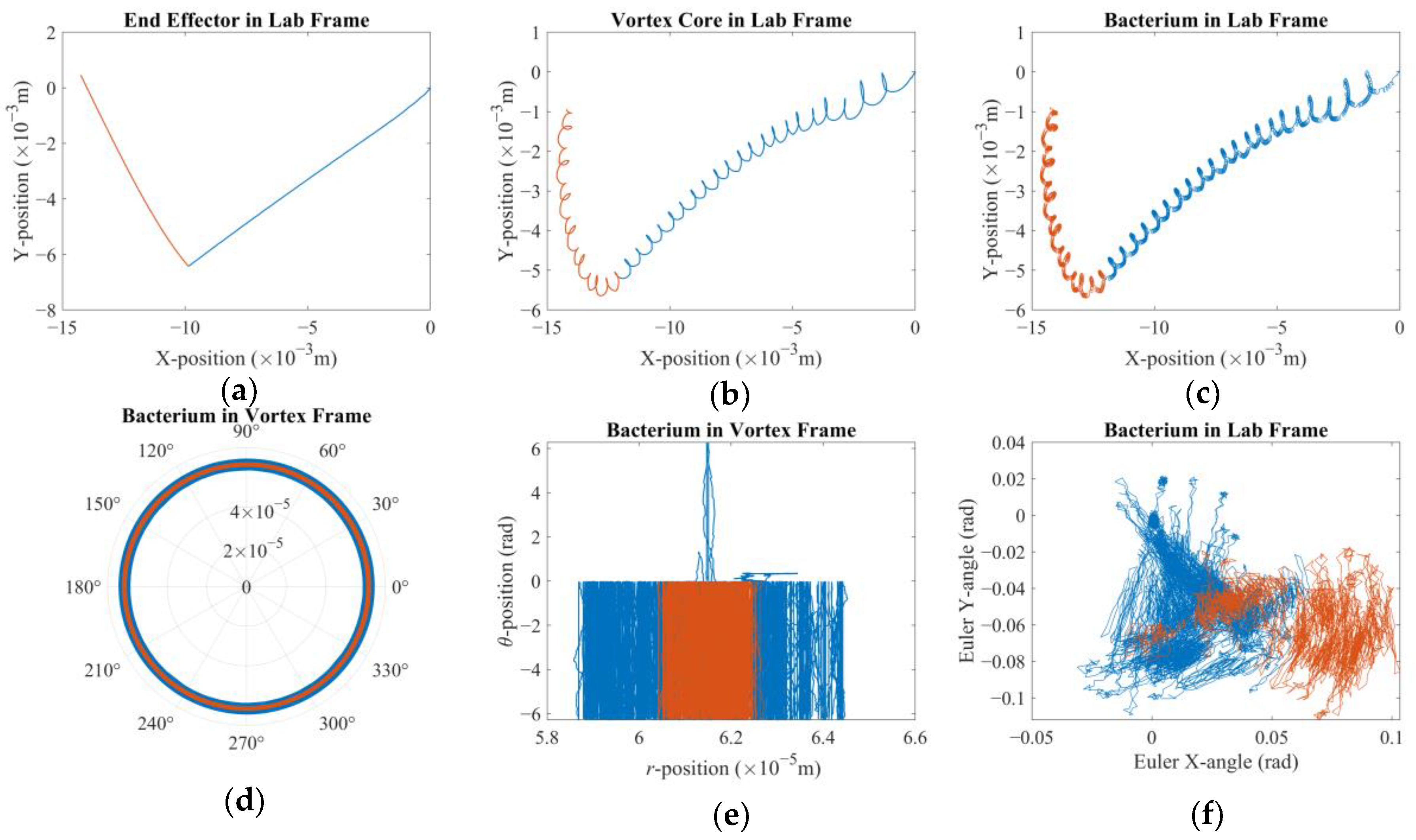
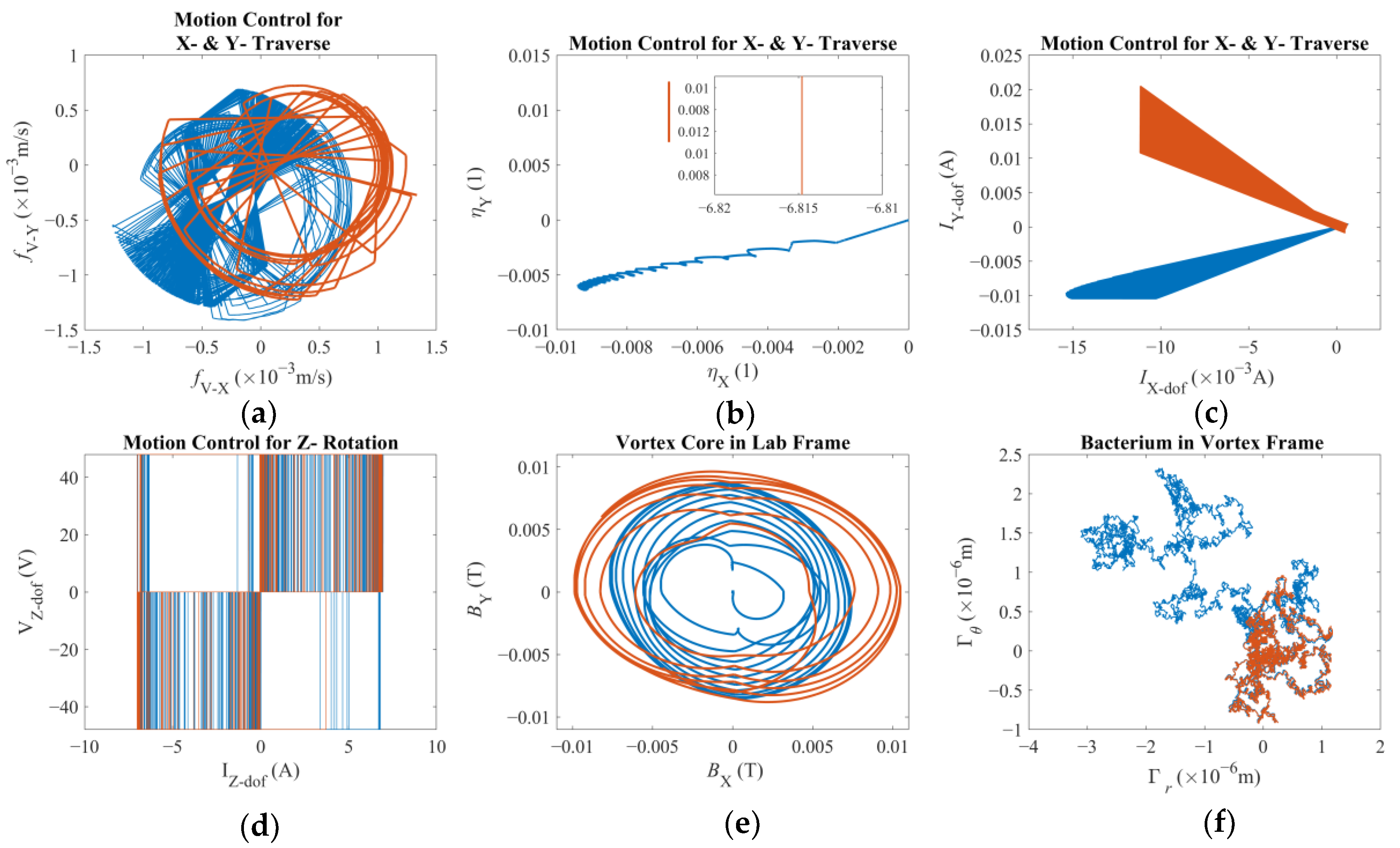
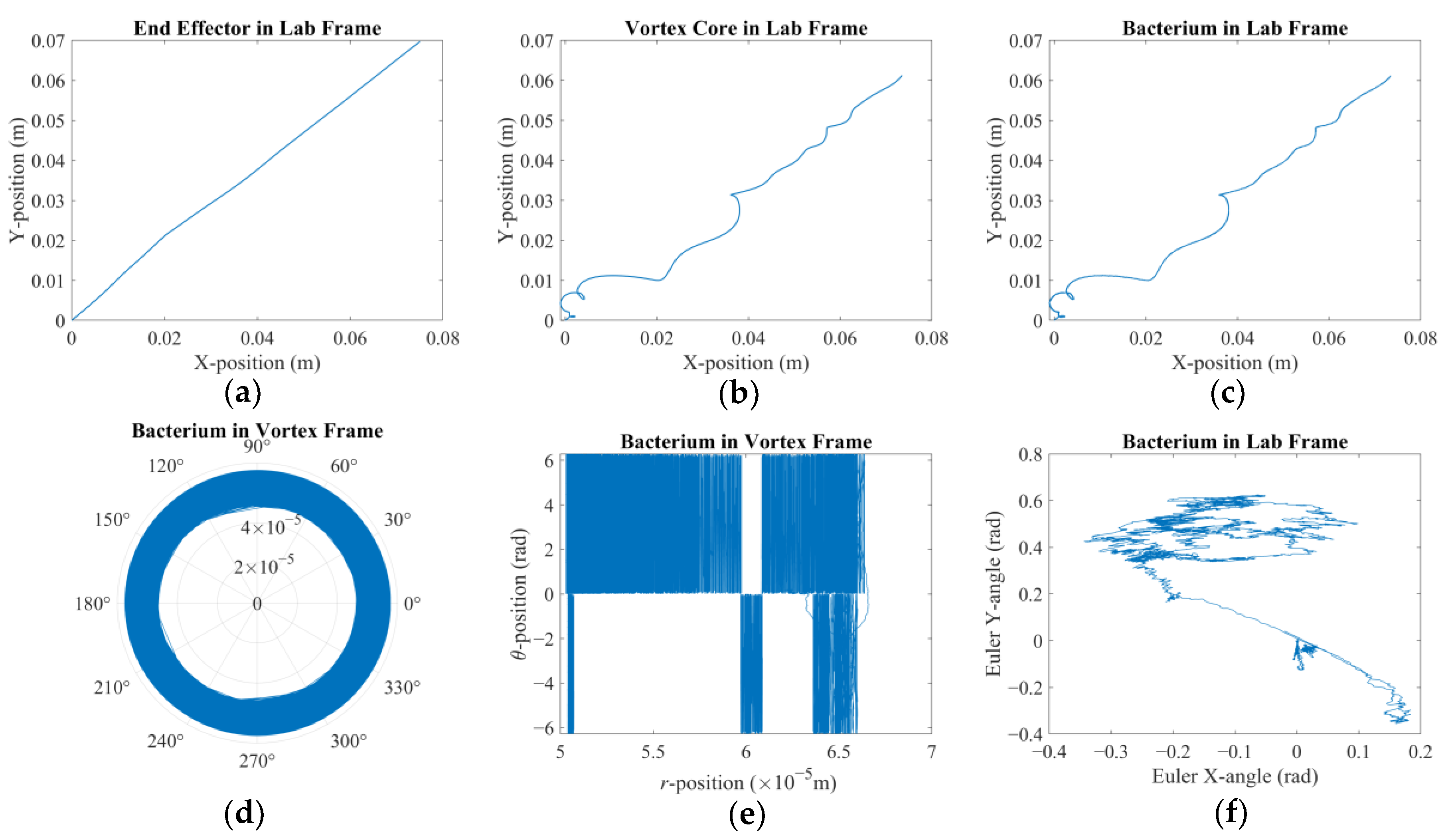
There are two results of this numerical investigation that could be of utmost importance for the future robotic studies of a similar kind. First, displacement and error plots clearly depict that the controller was not able to enforce the velocity reference, as the net displacement fell shorter than the expected value. However, the end-effector of the robotic arm and the vortex core were able to follow each other almost in unison, which, for this study, is the most important criterion in the manual search for control parameters. The velocity reference set to put the overall motion control performance to the test; however, the alignment between the end-effector and the vortex core should not deteriorate beyond what was observed. If two errors were not coupled, arguably, the results would have been completely different. If the error from the robotic arm is considered alone, the arm would have kept up with the velocity reference with higher accuracy but regardless of what happened to the spherical magnetic particle. In the opposite case, if only the error from the vortex is used, virtually, there would have been no limit to the traverse of the end-effector, except its own physical limits, because the error will only increase over time. In either case, one cannot guarantee the existence of the controlled forced vortex, as the distance between the axis of rotation of the third degree-of-freedom and the spherical magnetic particle could become too great for addressable manipulation. In such a case, as the vortex core might become virtually lost, the robotic system must home itself, i.e., search for the magnetic particle and reinitialize the rotation, and then look for the particle to tow, i.e., locate the particle and capture it again. If the particle is a single-celled organism, then simply backtracking the steps might not be enough to recover.
Second, the orbital velocity of the bacterium was deduced to be affected by the displacement direction of the vortex core. The bacterium can exhibit much faster or slower orbital velocities than expected, and even opposite in direction, owing to the step-out phenomenon. Although this requires further careful characterization to fully understand, the implication is promising for robotic applications: the directions of the rotation rate and traverse to the magnetic field would couple either to amplify or attenuate the apparent instantaneous strength of the forced vortex. The direction of the orbital motion might not be of consequence; however, this presented important future research to further ascertain the underlying physics. For instance, the fluid medium might be in motion, e.g., an upstream with a random profile might be present, which would result in a similar behavior. In either case, further numerical study is needed to confirm or dismiss this initial conclusion with a detailed parametric sweep of the relative velocity profile.
It is important to note that such micro-tweezer systems might arguably not be prone to the Brownian noise given that the magnetic field would dominate the overall motion, dampening the possible stochastic effects present. Nevertheless, the bacterium cell itself is subject to such processes, but this phenomenon is not directly included in the equation of motion because the equation set would have been transformed into stochastic differential equations requiring more sophisticated solvers and higher computational resources [
50], for the entire system is coupled given how the force and torque components are intricately coupled. Hence, the approach of superimposing the so-called random jumps on the calculated displacements at the end of each time-step was preferred instead.
In this study, it is assumed that all the sensory information was obtained with no latency and with high resolution. Indeed, the dedicated DC motor assemblies at the joints are normally expected to include proper encoders to supply the position and velocity information required for high-performance feedback control. The main question would be to obtain the position information on the vortex core. Depending on the working conditions, the system might defer to visual-serving via cameras [
51], fluorescent imaging [
52], or acoustics [
53]. Sensory equipment could be mounted on the robotic arm or positioned around the fluid medium based on the optimum noise-to-signal ratio. However, the use of magnetic sensing might arguably be almost completely ineffective due to the strong field emanating from the permanent magnets. Furthermore, multiple methods can be fused to track the vortex core and the towed particle. The size difference might even demand such applications as to pick up and release particles in an addressable and controllable manner.
The coefficients kp and ki used in this work were simply tuned for the robotic arm only. After which, the weighing coefficient, β, is tuned for the coupled error approach. A more robust and rigorous tuning would call for an optimization study on the steady-state error of the system. Furthermore, the former coefficients could be split into two separate sets, i.e., one set for the robotic arm and one set for the vortex core. This, in turn, would increase the demand for computational time and resources for the said optimization task, but more accurate solutions can be achieved.
Finally, the magnetic spherical particle might experience a net vertical force due to the gravitational pull, buoyancy, and gradient of the magnetic field. Here, in this study, equations are written for full six-degrees of freedom; however, these effects are cancelled out by numerically tuning the mass fraction of the resin–nanoparticle mixture. Lighter and heavier resin materials and different types of magnetic nanoparticles are available. Therefore, the nanoparticle content can be modified. The total number of paramagnetic nanoparticles will affect the overall magnetization behavior. Therefore, depending on the application parameters, such as the density or temperature of the fluid medium and the working distance of the permanent magnets, one should determine the optimum set of total volume, total mass, and overall magnetization of the spherical magnetic particle constituting the vortex core. Hence, this stands as a computationally demanding multi-variable multi-objective function design-optimization problem, which might demand case-specific attention. However, a mathematical model, such as the one presented here in this study, will be needed to carry out the said optimization task.


