
Investigation and Modeling of the Behavior of Temperature Characteristics of 0.3–1.1 GHz Complementary Metal Oxide Semiconductor Class-A Broadband Power Amplifiers


Abstract
1. Introduction
2. Methodology
3. Measurements
4. Results
4.1. S11
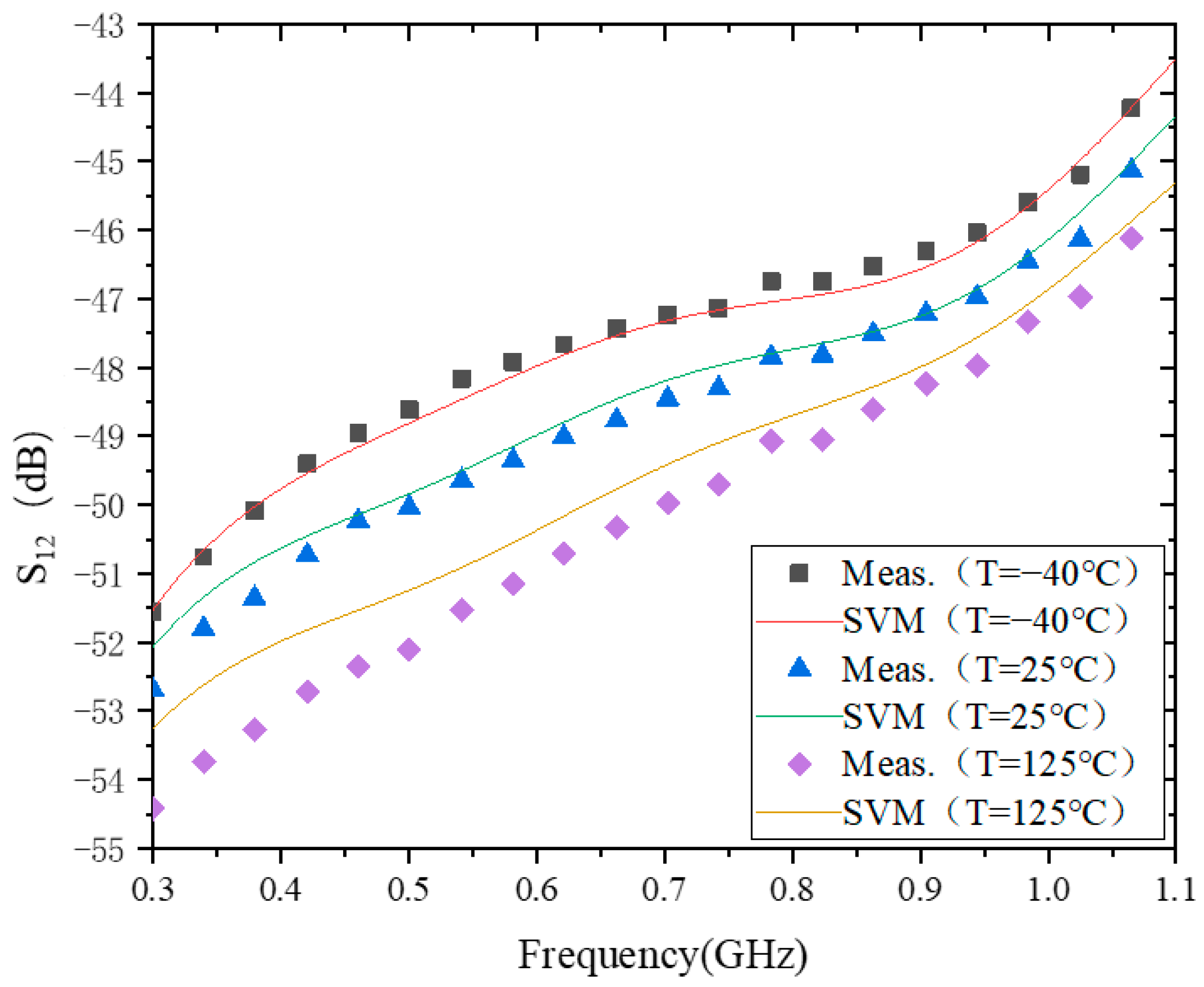
4.2. S12
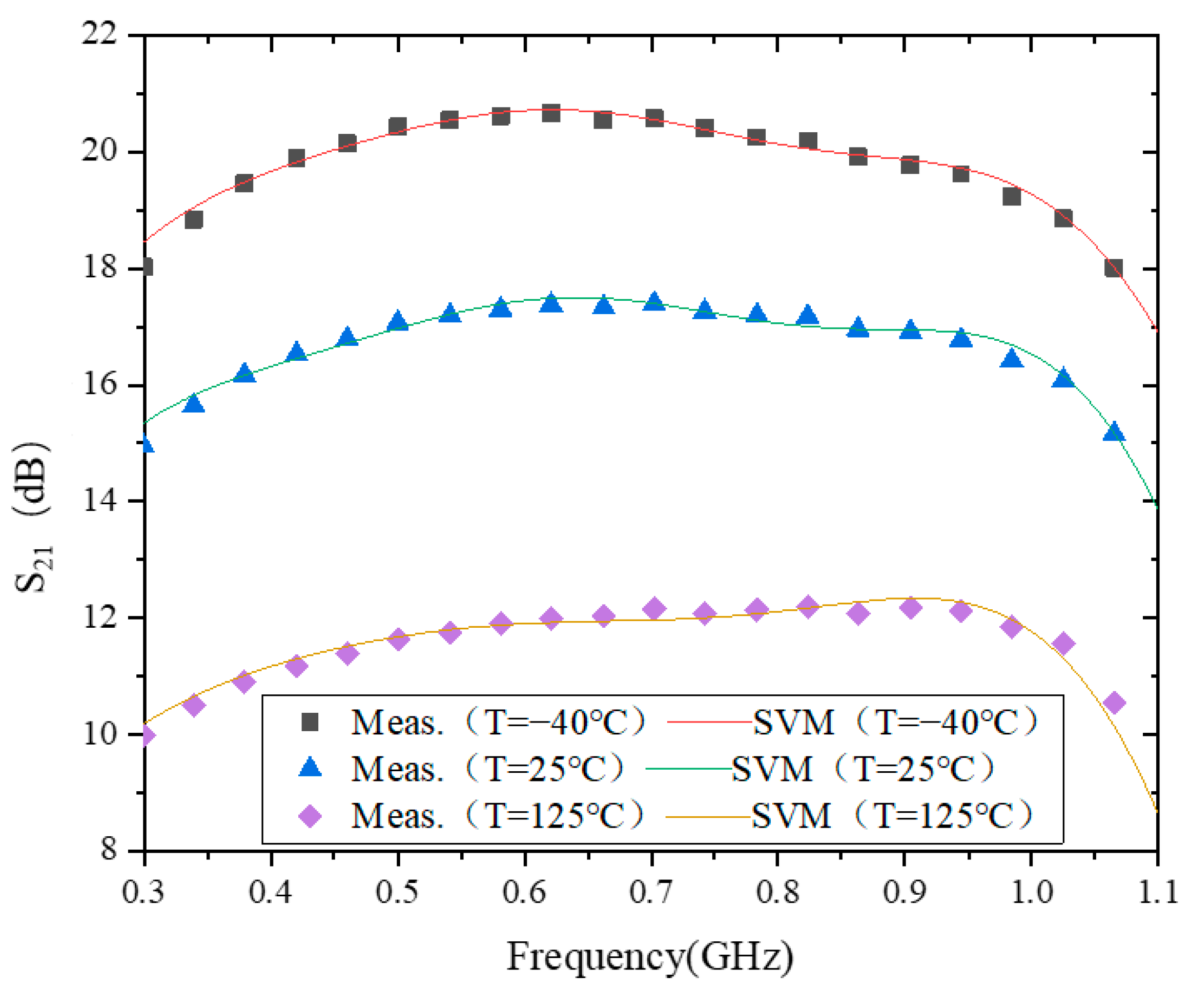
4.3. S21
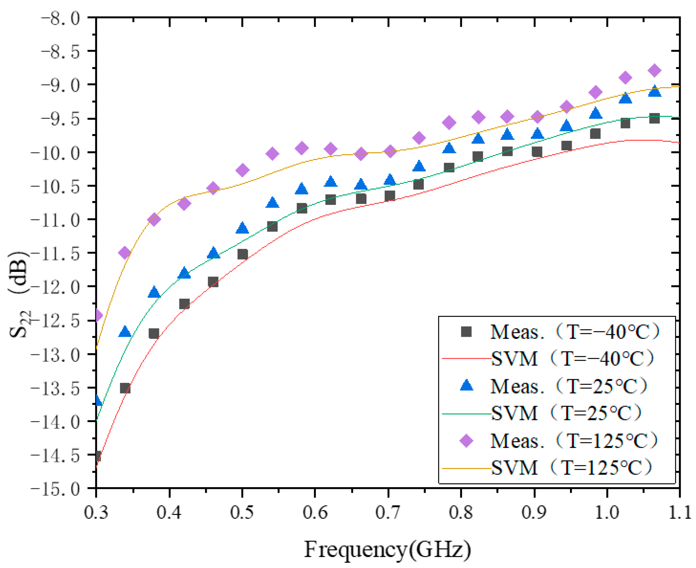
4.4. S22
5. Conclusions
Author Contributions
Funding
Data Availability Statement
Conflicts of Interest
References
- Amar, A.S.I.; Mamidanna, M.; Darwish, M.; El-Hennawy, H. High Gain Broadband Power Amplifier Design Based on Integrated Diplexing Networks. IEEE Microw. Wirel. Compon. Lett. 2022, 32, 133–136. [Google Scholar] [CrossRef]
- Piacibello, A.; Giofrè, R.; Quaglia, R.; Figueiredo, R.; Carvalho, N.; Colantonio, P.; Valenta, V.; Camarchia, V. A 5-W GaN Doherty Amplifier for Ka-Band Satellite Downlink With 4-GHz Bandwidth and 17-dB NPR. IEEE Microw. Wirel. Compon. Lett. 2022, 32, 964–967. [Google Scholar] [CrossRef]
- Rio, D.; Gurutzeaga, I.; Beriain, A.; Solar, H.; Berenguer, R. A Compact, Wideband, and Temperature Robust 67–90-GHz SiGe Power Amplifier with 30% PAE. IEEE Microw. Wirel. Compon. Lett. 2019, 29, 351–353. [Google Scholar]
- Zhou, S. Experimentally investigating the degradations of the GaN PA indexes under different temperature conditions. Microw. Opt. Technol. Lett. 2021, 63, 758–763. [Google Scholar] [CrossRef]
- Yu, C.; Yuan, J.S. Electrical and Temperature Stress Effects on Class-AB Power Amplifier Performances. IEEE Trans. Electron Devices 2007, 54, 1346–1350. [Google Scholar]
- Zhou, S.H. Experimental investigation on the performance degradations of the GaN class-F power amplifier under humidity conditions. Semicond. Sci. Technol. 2021, 36, 035025. [Google Scholar] [CrossRef]
- Zhou, S.; Yang, C.; Wang, J. Support Vector Machine–Based Model for 2.5–5.2 GHz CMOS Power Amplifier. Micromachines 2022, 13, 1012. [Google Scholar] [CrossRef] [PubMed]
- Cortes, C.; Vapnik, V. Support-vector network. Mach. Learn. 1995, 20, 273–297. [Google Scholar] [CrossRef]
- Boser, B.; Guyon, I.; Vapnik, V. A training algorithm for optimal margin classifiers. In Proceedings of the Fifth Annual Workshop on Computational Learning Theory, Pittsburgh, PA, USA, 27–29 July 1992; pp. 144–152. [Google Scholar]
- Chen, Y.; Mao, Q.; Wang, B.; Duan, P.; Zhang, B.; Hong, Z. Privacy-Preserving Multi-Class Support Vector Machine Model on Medical Diagnosis. IEEE J. Biomed. Health Inform. 2022, 26, 3342–3353. [Google Scholar] [CrossRef] [PubMed]
- Gupta, C.; Rao, K.V.S.R.; Datta, P. Support Vector Machine Based Prediction of Work-Life Balance among Women in Information Technology Organizations. IEEE Eng. Manag. Rev. 2022, 50, 147–155. [Google Scholar] [CrossRef]
- Liu, T.; Zhu, H.; Wu, M.; Zhang, W. Rotor Displacement Self-Sensing Method for Six-Pole Radial Hybrid Magnetic Bearing Using Mixed-Kernel Fuzzy Support Vector Machine. IEEE Trans. Appl. Supercond. 2020, 30, 3603404. [Google Scholar] [CrossRef]
- Eke, C.S.; Jammeh, E.; Li, X.; Carroll, C.; Pearson, S.; Ifeachor, E. Early Detection of Alzheimer’s Disease with Blood Plasma Proteins Using Support Vector Machines. IEEE J. Biomed. Health Inform. 2021, 25, 218–226. [Google Scholar] [CrossRef] [PubMed]
- Lu, H.; Guo, W.; Su, C.; Li, X.; Lu, Y.; Chen, Z.; Zhu, L. Optimization on Adhesive Stamp Mass-Transfer of Micro-LEDs with Support Vector Machine Model. IEEE J. Electron Devices Soc. 2020, 8, 554–558. [Google Scholar] [CrossRef]
- Huang, J.; Jiang, B.; Xu, C.; Wang, N. Slipping Detection of Electric Locomotive Based on Empirical Wavelet Transform, Fuzzy Entropy Algorithm and Support Vector Machine. IEEE Trans. Veh. Technol. 2021, 70, 7558–7570. [Google Scholar] [CrossRef]
- Chen, P.; Brazil, T.J. Classifying load-pull contours of a broadband high-efficiency power amplifier using a support vector machine. In Proceedings of the 2017 Integrated Nonlinear Microwave and Millimetre-Wave Circuits Workshop (INMMiC), Graz, Austria, 20–21 April 2017; pp. 1–3. [Google Scholar] [CrossRef]
- Hu, G.; Zhu, X.-W.; Xia, J.; Yu, C.; Shi, Y. A Vector Rotation-based Nonlinear Support Vector Regression Model for Envelope Tracking RF Power Amplifiers. In Proceedings of the 2019 International Conference on Microwave and Millimeter Wave Technology (ICMMT), Guangzhou, China, 19–22 May 2019; pp. 1–3. [Google Scholar] [CrossRef]
- Xu, J.; Jiang, W.; Ma, L.; Li, M.; Yu, Z.; Geng, Z. Augmented Time-Delay Twin Support Vector Regression-Based Behavioral Modeling for Digital Predistortion of RF Power Amplifier. IEEE Access 2019, 7, 59832–59843. [Google Scholar] [CrossRef]
- Abegaz, K.H.; Etikan, İ. Artificial Intelligence-Driven Ensemble Model for Predicting Mortality Due to COVID-19 in East Africa. Diagnostics 2022, 12, 2861. [Google Scholar] [CrossRef] [PubMed]
- Zhang, H.; Han, Y. A New Mixed-Gas-Detection Method Based on a Support Vector Machine Optimized by a Sparrow Search Algorithm. Sensors 2022, 22, 8977. [Google Scholar] [CrossRef] [PubMed]
- Zaki, A.; Métwalli, A.; Aly, M.H.; Badawi, W.K. Wireless Communication Channel Scenarios: Machine-Learning-Based Identification and Performance Enhancement. Electronics 2022, 11, 3253. [Google Scholar] [CrossRef]
- Tan, S.; Pan, J.; Zhang, J.; Liu, Y. CASVM: An Efficient Deep Learning Image Classification Method Combined with SVM. Appl. Sci. 2022, 12, 11690. [Google Scholar] [CrossRef]
- Lin, W.-M.; Wu, C.-H. Fast Support Vector Machine for Power Quality Disturbance Classification. Appl. Sci. 2022, 12, 11649. [Google Scholar] [CrossRef]
- Razavi, B. Design of Analog CMOS Integrated Circuits; McGraw Hill Higher Education: New York, NY, USA, 2003; pp. 17–21. [Google Scholar]
- Neamen, D.A. Semiconductor Physics and Devices: Basic Principles; McGraw Hill Higher Education: New York, NY, USA, 2012; pp. 395–419. [Google Scholar]
- Lee, T.H. The Design of CMOS Radio-Frequency Integrated Circuits; Cambridge University Press: Cambridge, UK, 2012; pp. 172–189. [Google Scholar]
- Mišić, J.; Marković, V.; Marinković, Z.; Budimir, D. Behavioral modeling of low noise amplifiers for LTE systems based on modified Elman neural networks. In Proceedings of the 2014 22nd Telecommunications Forum Telfor (TELFOR), Belgrade, Serbia, 25–27 November 2014; pp. 308–311. [Google Scholar] [CrossRef]
- Shah, J.; Patel, H.; Gajjar, R.; Panchal, D.; Patel, M.I. Aspect Ratio Estimation for MOS Amplifier using Machine Learning. In Proceedings of the 2021 IEEE 2nd International Conference on Applied Electromagnetics, Signal Processing, & Communication (AESPC), Bhubaneswar, India, 26–28 November 2021; pp. 1–6. [Google Scholar] [CrossRef]


| Specification | 0.3–1.1 GHz CMOS PA | |||||||||
|---|---|---|---|---|---|---|---|---|---|---|
| Temperature | Training Time (ms) | Training Error (MSE) | Test Error (MSE) | |||||||
| SVM | Elman | GRNN | SVM | Elman | GRNN | SVM | Elman | GRNN | ||
| S11 | −40 °C | 13.1828 | 22.0649 | 14.5207 | 7.6094 × 10⁻² | 1.3545 × 10⁻¹ | 8.7519 × 10⁻¹ | 7.5948 × 10⁻² | 1.3329 × 10⁻¹ | 8.1818 × 10⁻¹ |
| 25 °C | 13.1884 | 21.7823 | 14.4215 | 1.4338 × 10⁻¹ | 1.5737 × 10⁻¹ | 5.0432 × 10⁻¹ | 1.4313 × 10⁻¹ | 1.5638 × 10⁻¹ | 4.9011 × 10⁻¹ | |
| 125 °C | 13.3785 | 21.8585 | 14.4760 | 2.3635 × 10⁻² | 2.3901 × 10⁻² | 1.2462 × 10⁻¹ | 2.3117 × 10⁻² | 2.3299 × 10⁻² | 1.2311 × 10⁻¹ | |
| S12 | −40 °C | 13.0228 | 21.9445 | 14.2185 | 4.4906 × 10⁻¹ | 1.2736 | 5.8912 × 10⁻¹ | 4.3359 × 10⁻¹ | 1.2522 | 5.6253 × 10⁻¹ |
| 25 °C | 13.1254 | 24.2897 | 13.2567 | 4.4344 × 10⁻¹ | 5.3769 × 10⁻¹ | 5.9591 × 10⁻¹ | 4.4285 × 10⁻¹ | 5.3987 × 10⁻¹ | 5.7790 × 10⁻¹ | |
| 125 °C | 13.1286 | 21.9958 | 13.5437 | 1.8640 | 1.9003 | 2.3674 | 1.6438 | 1.8353 | 2.9581 | |
| S21 | −40 °C | 13.2321 | 21.7983 | 13.3256 | 1.9315 × 10⁻¹ | 4.7687 × 10⁻¹ | 3.8398 × 10⁻¹ | 1.9177 × 10⁻¹ | 4.5078 × 10⁻¹ | 3.5495 × 10⁻¹ |
| 25 °C | 13.3907 | 21.9360 | 13.4565 | 2.1798 × 10⁻¹ | 3.0310 × 10⁻¹ | 3.3669 × 10⁻¹ | 2.1655 × 10⁻¹ | 2.7566 × 10⁻¹ | 3.0555 × 10⁻¹ | |
| 125 °C | 13.335 | 21.8518 | 13.769 | 4.2989 × 10⁻¹ | 4.5583 × 10⁻¹ | 4.7763 × 10⁻¹ | 4.2388 × 10⁻¹ | 4.6239 × 10⁻¹ | 4.4368 × 10⁻¹ | |
| S22 | −40 °C | 13.1499 | 30.5666 | 15.0396 | 1.8651 × 10⁻¹ | 4.2107 × 10⁻¹ | 3.3053 × 10⁻¹ | 1.8112 × 10⁻¹ | 4.1284 × 10⁻¹ | 3.2324 × 10⁻¹ |
| 25 °C | 13.3284 | 25.0988 | 14.0633 | 1.9128 × 10⁻¹ | 4.9093 × 10⁻¹ | 2.4705 × 10⁻¹ | 1.9015 × 10⁻¹ | 4.8292 × 10⁻¹ | 2.4147 × 10⁻¹ | |
| 125 °C | 13.1787 | 23.5633 | 13.9547 | 2.2977 × 10⁻¹ | 3.2298 × 10⁻¹ | 2.5628 × 10⁻¹ | 2.2803 × 10⁻¹ | 3.1423 × 10⁻¹ | 2.5102 × 10⁻¹ | |
Disclaimer/Publisher’s Note: The statements, opinions and data contained in all publications are solely those of the individual author(s) and contributor(s) and not of MDPI and/or the editor(s). MDPI and/or the editor(s) disclaim responsibility for any injury to people or property resulting from any ideas, methods, instructions or products referred to in the content. |
© 2024 by the authors. Licensee MDPI, Basel, Switzerland. This article is an open access article distributed under the terms and conditions of the Creative Commons Attribution (CC BY) license (https://creativecommons.org/licenses/by/4.0/).
Share and Cite
Li, R.; Zhou, S.; Yang, C.; Wang, J. Investigation and Modeling of the Behavior of Temperature Characteristics of 0.3–1.1 GHz Complementary Metal Oxide Semiconductor Class-A Broadband Power Amplifiers. Micromachines 2024, 15, 246. https://doi.org/10.3390/mi15020246
Li R, Zhou S, Yang C, Wang J. Investigation and Modeling of the Behavior of Temperature Characteristics of 0.3–1.1 GHz Complementary Metal Oxide Semiconductor Class-A Broadband Power Amplifiers. Micromachines. 2024; 15(2):246. https://doi.org/10.3390/mi15020246
Chicago/Turabian StyleLi, Ruiliang, Shaohua Zhou, Cheng Yang, and Jian Wang. 2024. "Investigation and Modeling of the Behavior of Temperature Characteristics of 0.3–1.1 GHz Complementary Metal Oxide Semiconductor Class-A Broadband Power Amplifiers" Micromachines 15, no. 2: 246. https://doi.org/10.3390/mi15020246
APA StyleLi, R., Zhou, S., Yang, C., & Wang, J. (2024). Investigation and Modeling of the Behavior of Temperature Characteristics of 0.3–1.1 GHz Complementary Metal Oxide Semiconductor Class-A Broadband Power Amplifiers. Micromachines, 15(2), 246. https://doi.org/10.3390/mi15020246