

Thermal Flow Meter with Integrated Thermal Conductivity Sensor

 , , ,
, , ,
Abstract
1. Introduction
2. Design and Operating Principle
2.1. Thermal Flow Sensor
2.2. Thermal Conductivity Sensor
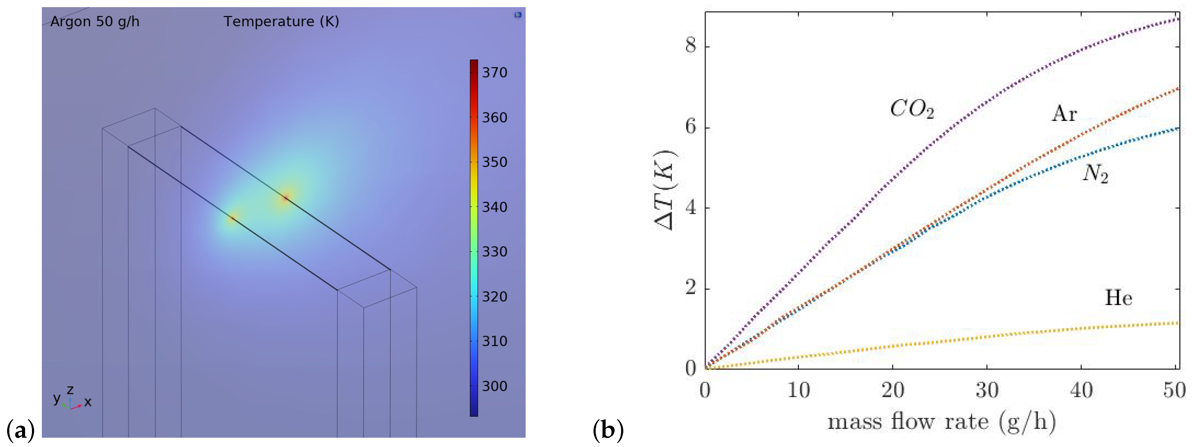
3. Simulation
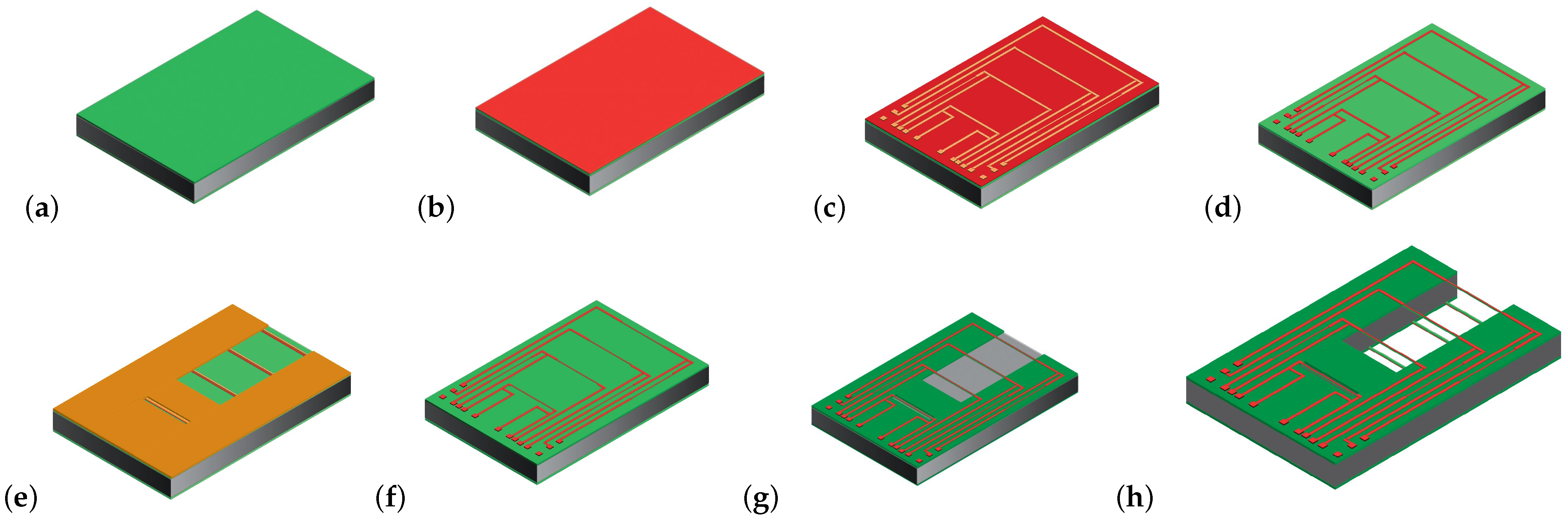
4. Fabrication
5. Results and Discussion
5.1. Thermal Conductivity Sensor
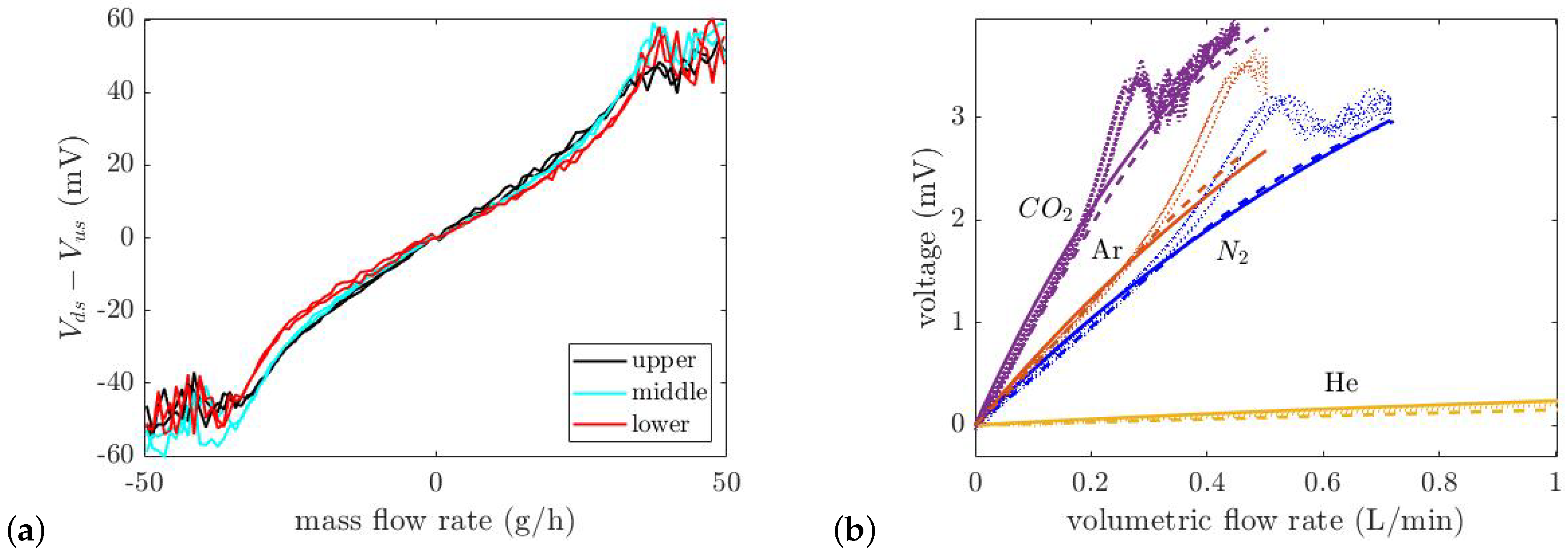
5.2. Thermal Flow Sensor
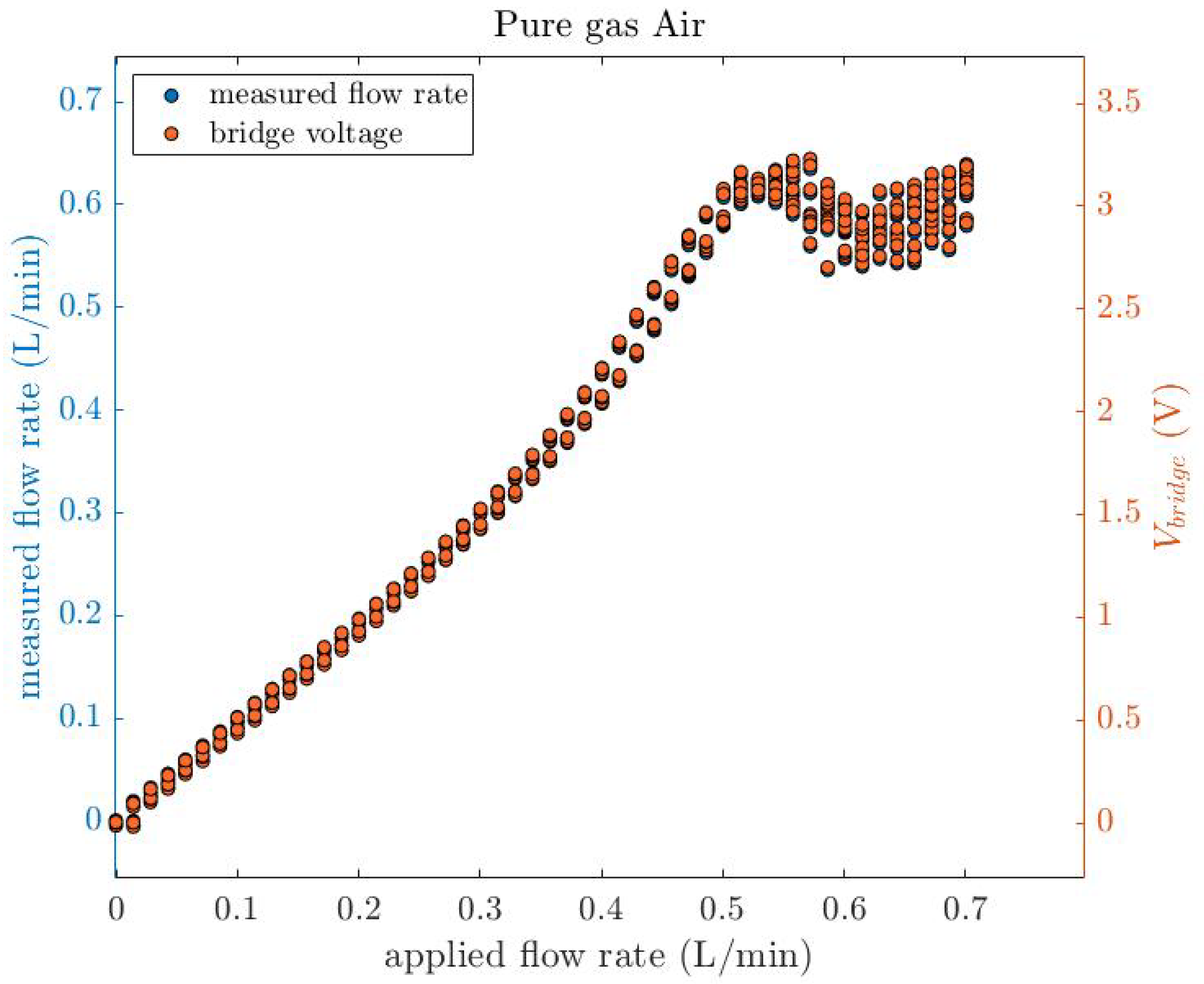
5.3. Simultaneous Measurement of Flow Rate and Thermal Conductivity
6. Conclusions
Author Contributions
Funding
Data Availability Statement
Conflicts of Interest
References
- Balakrishnan, V.; Phan, H.P.; Dinh, T.; Dao, D.V.; Nguyen, N.T. Thermal Flow Sensors for Harsh Environments. Sensors 2017, 17, 2061. [Google Scholar] [CrossRef] [PubMed]
- King, L.V. On The Convection of Heat From Small Cylinders in A Stream Of Fluid: Determination of the Convection Constants of Small Platinum Wires with Applications to Hot-wire Anemometry. Philos. Trans. R. Soc. Lond. Ser. A Contain. Pap. Math. Phys. Character 1914, 214, 373–432. [Google Scholar]
- Van Oudheusden, B.W. Silicon Thermal Flow Sensors. Sens. Actuators A Phys. 1992, 30, 5–26. [Google Scholar] [CrossRef]
- Elwenspoek, M. Thermal Flow Micro Sensors. In Proceedings of the 1999 International Semiconductor Conference (Cat. No. 99TH8389), Sinaia, Romania, 5–9 October 1999; Volume 17, pp. 423–435. [Google Scholar]
- Khan, B. A Comparative Analysis of Thermal Flow Sensing In Biomedical Applications. Int. J. Biomed. Eng. Sci. 2016, 3, 1–7. [Google Scholar] [CrossRef]
- Kuo, J.T.W.; Yu, L.; Meng, E. Micromachined Thermal Flow Sensors—A Review. Micromachines 2012, 3, 550–573. [Google Scholar] [CrossRef]
- Van Oudheusden, B. Silicon flow sensors. IEE Proc. D Control Theory Appl. 1988, 135, 373–380. [Google Scholar] [CrossRef]
- Chung, W.S.; Kwon, O.; Park, S.; Choi, Y.K.; Lee, J.S. Tunable AC Thermal Anemometry. Superlattices Microstruct. 2004, 35, 325–338. [Google Scholar] [CrossRef]
- Heyd, R.; Hadaoui, A.; Fliyou, M.; Koumina, A.; Ameziane, E.L.; Outzourit, A.; Saboungi, M. Development of Absolute Hot-wire Anemometry by the 3ω Method. Rev. Sci. Instrum. 2010, 81, 1–6. [Google Scholar] [CrossRef] [PubMed]
- Gauthier, S.; Giani, A.; Combette, P. Gas thermal conductivity measurement using the three-omega method. Sens. Actuators A 2013, 195, 50–55. [Google Scholar]
- Kuntner, J.; Kohl, F.; Jakoby, B. Simultaneous Thermal Conductivity and Diffusivity Sensing in Liquids Using a Micromachined Device. Sens. Actuators A Phys. 2006, 130, 62–67. [Google Scholar] [CrossRef]
- Beigelbeck, R.; Kohl, F.; Cerimovic, S.; Talic, A.; Kelinger, F.; Jakoby, B. Thermal Property Determination of Laminar-flowing Fluids Utilizing the Frequency Response of a Calorimetric Flow Sensor. In Proceedings of the SENSORS, 2008 IEEE, Lecce, Italy, 26–29 October 2008; pp. 518–521. [Google Scholar]
- Beigelbeck, R.; Nachtnebel, H.; Kohl, F.; Jakoby, B. A Novel Measurement Method for the Thermal Properties of Liquids by Utilizing a Bridge-based Micromachined Sensor. Meas. Sci. Technol. 2011, 22, 1–9. [Google Scholar] [CrossRef]
- Hepp, C.J.; Krogmann, F.T.; Polak, J.; Lehmann, M.M.; Urban, G.A. AC Characterisation of Thermal Flow Sensor with Fluid Characterisation Feature. In Proceedings of the 2011 16th International Solid-State Sensors, Actuators and Microsystems Conference, Beijing, China, 5–9 June 2011; pp. 1084–1087. [Google Scholar]
- Reyes Romero, D.F. Development of a Medium Independent Flow Measurement Technique Based on Oscillatory Thermal Excitation. Ph.D. Thesis, University of Freiburg, Freiburg, Germany, 2014. [Google Scholar]
- Zhu, Y.Q.; Hepp, C.J.; Urban, G.A. Modelling and Simulation of a Thermal Flow Sensor For Determining the Flow Speed and Thermal Properties of Binary Gas Mixtures. Eurosensors 2016, 168, 1028–1031. [Google Scholar] [CrossRef]
- Hepp, C.J.; Krogmann, F.T.; Urban, G.A. Flow rate independent sensing of thermal conductivity in a gas stream by a thermal MEMS-sensor—Simulation and experiments. Sens. Actuators A 2017, 253, 136–145. [Google Scholar] [CrossRef]
- Van Baar, J.J.; Wiegerink, R.J.; Lammerink, T.S.; Krijnen, G.J.; Elwenspoek, M. Micromachined Structures for Thermal Measurements of Fluid and Flow Parameters. J. Micromech. Microeng. 2001, 11, 311–318. [Google Scholar] [CrossRef]
- Wang, J.; Liu, Y.; Zhou, H.; Wang, Y.; Wu, M.; Huang, G.; Li, T. Thermal Conductivity Gas Sensor with Enhanced Flow-Rate Independence. Sensors 2022, 22, 1308. [Google Scholar] [CrossRef] [PubMed]
- Joost, C.; Lammerink, T.S.; Groenesteijn, J.; Haneveld, J.; Wiegerink, R.J. Integrated Thermal and Microcoriolis Flow Sensing System with a Dynamic Flow Range of More Than Five Decades. Micromachines 2012, 3, 194–203. [Google Scholar] [CrossRef]
- Lötters, J.C.; van der Wouden, E.; Groenesteijn, J.; Sparreboom, W.; Lammerink, T.S.J.; Wiegerink, R.J. Integrated Multi-Parameter Flow Measurement System. In Proceedings of the 2014 IEEE 27th International Conference on Micro Electro Mechanical Systems (MEMS), San Francisco, CA, USA, 26–30 January 2014; pp. 975–978. [Google Scholar]
- Van der Wouden, E.; Groenesteijn, J.; Wiegerink, R.; Lötters, J. Egbert van der Wouden, Multi Parameter Flow Meter for On-Line Measurement of Gas Mixture Composition. Micromachines 2015, 6, 452–461. [Google Scholar] [CrossRef]
- Kenari, S.A.; Wiegerink, R.J.; Sanders, R.G.; Lotters, J.C. Towards A Gas Independent Thermal Flow Meter. In Proceedings of the 2023 IEEE 36th International Conference on Micro Electro Mechanical Systems (MEMS), Munich, Germany, 15–19 January 2023. [Google Scholar]
- De Bree, H.E.; Jansen, H.V.; Lammerink, T.S.; Krijnen, G.J.; Elwenspoek, M. Hans-Elias de Bree, Bi-directional Fast Flow Sensor with A Large Dynamic Range. J. Micromech. Microeng. 1998, 9, 186–189. [Google Scholar] [CrossRef]
- Lammerink, T.S.J.; Tas, N.R.; Elwenspoek, M.; Fluitman, J.H.J. Micro-liquid Flow Sensor. Sens. Actuators A 1993, 37, 45–50. [Google Scholar]
- Vangbo, M.; Baecklund, Y. Precise Mask Alignment to the Crystallographic Orientation of Silicon Wafers Using Wet Anisotropic Etching. J. Micromech. Microeng. 1996, 6, 279–284. [Google Scholar] [CrossRef]
- FLUIDAT. Available online: https://www.fluidat.com/default.asp (accessed on 20 April 2023).


| Parameter | Term | Value |
|---|---|---|
| Beam length | l | 2000 m |
| Beam width | w | 5 m |
| Silicon wafer thickness | 380 m | |
| V-groove width | 40 m | |
| V-groove length | 2000 m | |
| Chip width | - | 7500 m |
| Chip length | - | 11,500 m |
| Channel diameter | 2 cm | |
| Channel length | 10 cm | |
| V-groove depth | d | 28 m |
| Effective V-groove depth | 15 m | |
| Input current | I | 5 mA |
| Ambient temperature | 293 K | |
| Ambient resistance | 300 |
| Gas | He | N2 | Ar | CO2 |
|---|---|---|---|---|
| Voltage (V) | 1.55 | 1.71 | 1.81 | 1.83 |
| Coefficients | a [m·K/A] | b [m·K/W] |
|---|---|---|
| 189.4278 | −287.6934 |
| Gas | CO2 | N2 | Air | Ar | He |
|---|---|---|---|---|---|
| Sensitivity (mV/L/min) | 10.41 | 5.91 | 5.09 | 4.96 | 0.31 |
| Gas Physical Properties | CO2 | Ar | Air | N2 | He |
|---|---|---|---|---|---|
| Thermal conductivity (W/m·K) | 0.01652 | 0.01763 | 0.02598 | 0.026 | 0.1554 |
| Density (kg/m) | 1.84 | 1.662 | 1.189 | 1.165 | 0.1664 |
| Heat capacity (J/kg·K) | 846.8 | 521.9 | 1006 | 1043 | 5196 |
Disclaimer/Publisher’s Note: The statements, opinions and data contained in all publications are solely those of the individual author(s) and contributor(s) and not of MDPI and/or the editor(s). MDPI and/or the editor(s) disclaim responsibility for any injury to people or property resulting from any ideas, methods, instructions or products referred to in the content. |
© 2023 by the authors. Licensee MDPI, Basel, Switzerland. This article is an open access article distributed under the terms and conditions of the Creative Commons Attribution (CC BY) license (https://creativecommons.org/licenses/by/4.0/).
Share and Cite
Azadi Kenari, S.; Wiegerink, R.J.; Veltkamp, H.-W.; Sanders, R.G.P.; Lötters, J.C. Thermal Flow Meter with Integrated Thermal Conductivity Sensor. Micromachines 2023, 14, 1280. https://doi.org/10.3390/mi14071280
Azadi Kenari S, Wiegerink RJ, Veltkamp H-W, Sanders RGP, Lötters JC. Thermal Flow Meter with Integrated Thermal Conductivity Sensor. Micromachines. 2023; 14(7):1280. https://doi.org/10.3390/mi14071280
Chicago/Turabian StyleAzadi Kenari, Shirin, Remco J. Wiegerink, Henk-Willem Veltkamp, Remco G. P. Sanders, and Joost C. Lötters. 2023. "Thermal Flow Meter with Integrated Thermal Conductivity Sensor" Micromachines 14, no. 7: 1280. https://doi.org/10.3390/mi14071280
APA StyleAzadi Kenari, S., Wiegerink, R. J., Veltkamp, H.-W., Sanders, R. G. P., & Lötters, J. C. (2023). Thermal Flow Meter with Integrated Thermal Conductivity Sensor. Micromachines, 14(7), 1280. https://doi.org/10.3390/mi14071280