Characterization of Chaotic Electroconvection near Flat Inert Electrodes under Oscillatory Voltages

Abstract
1. Introduction
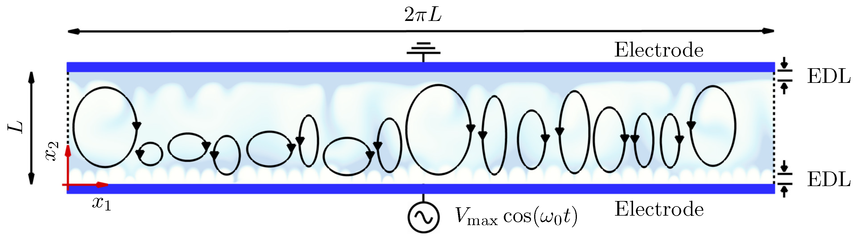
2. Problem Setup
3. Numerical Methods
4. Results
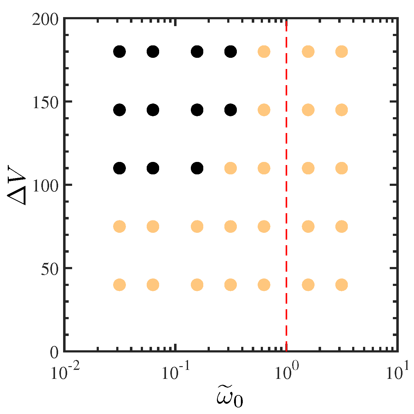
4.1. Electroconvective Instability of Binary Symmetric Electrolytes ()
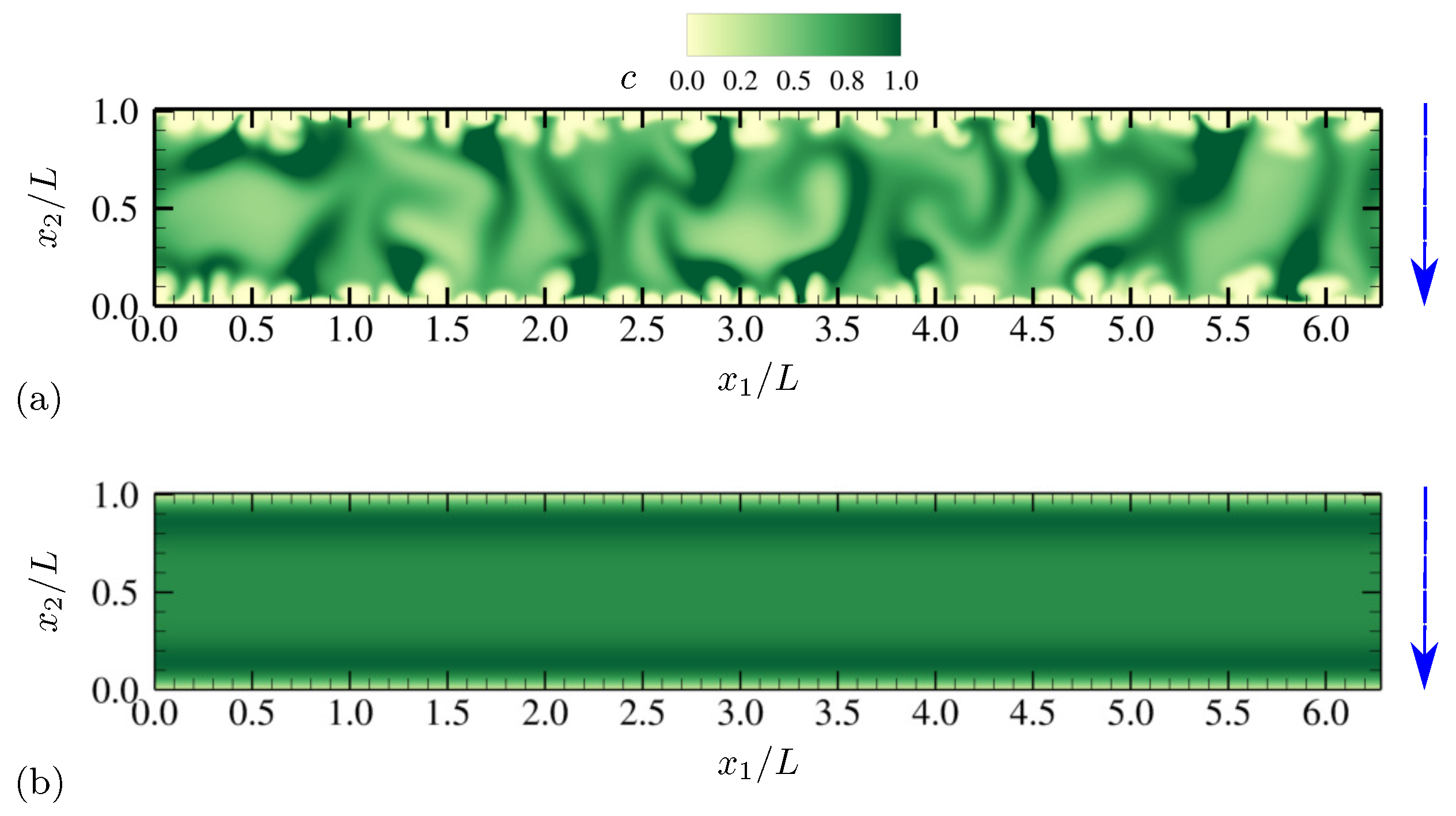
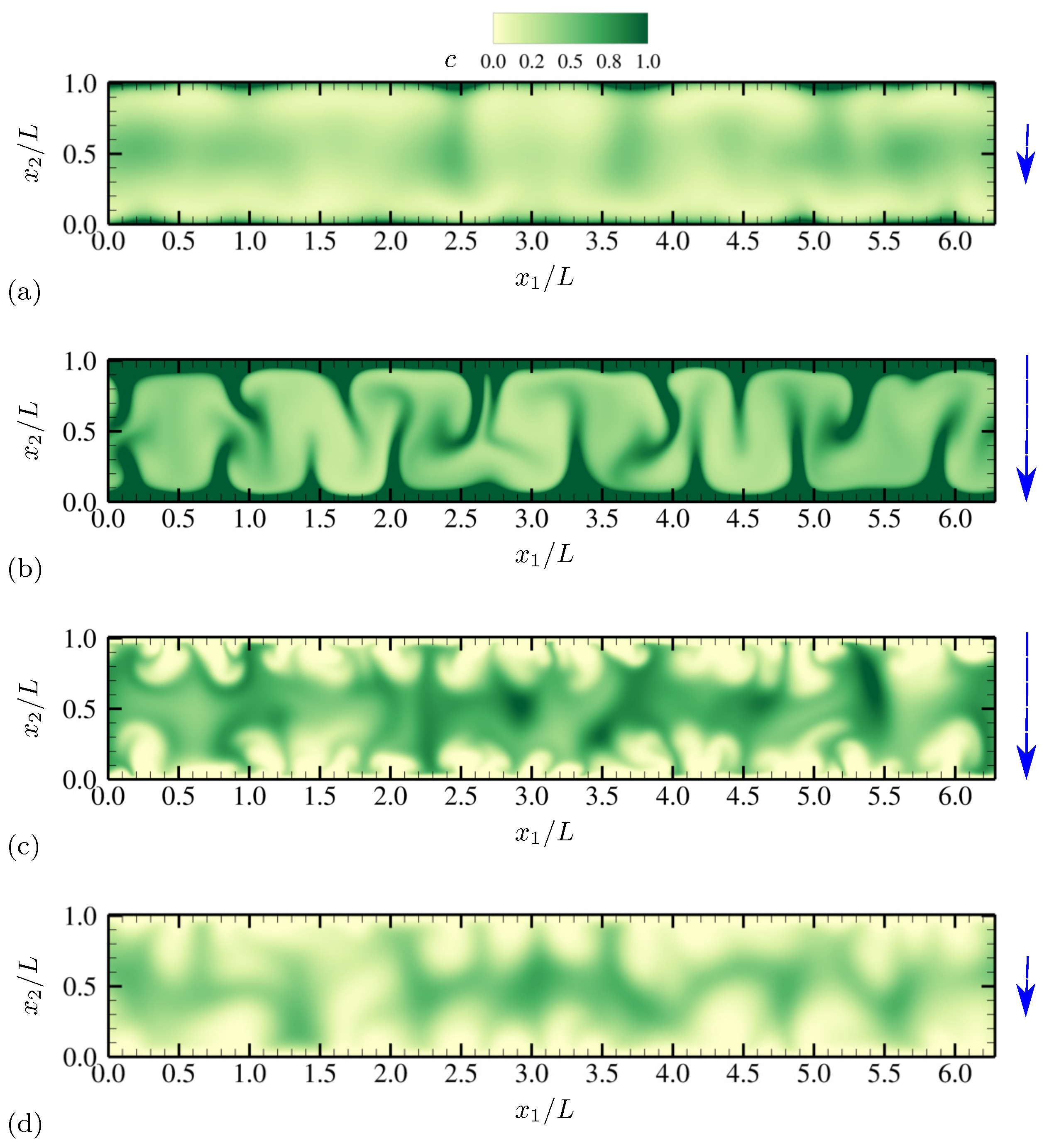
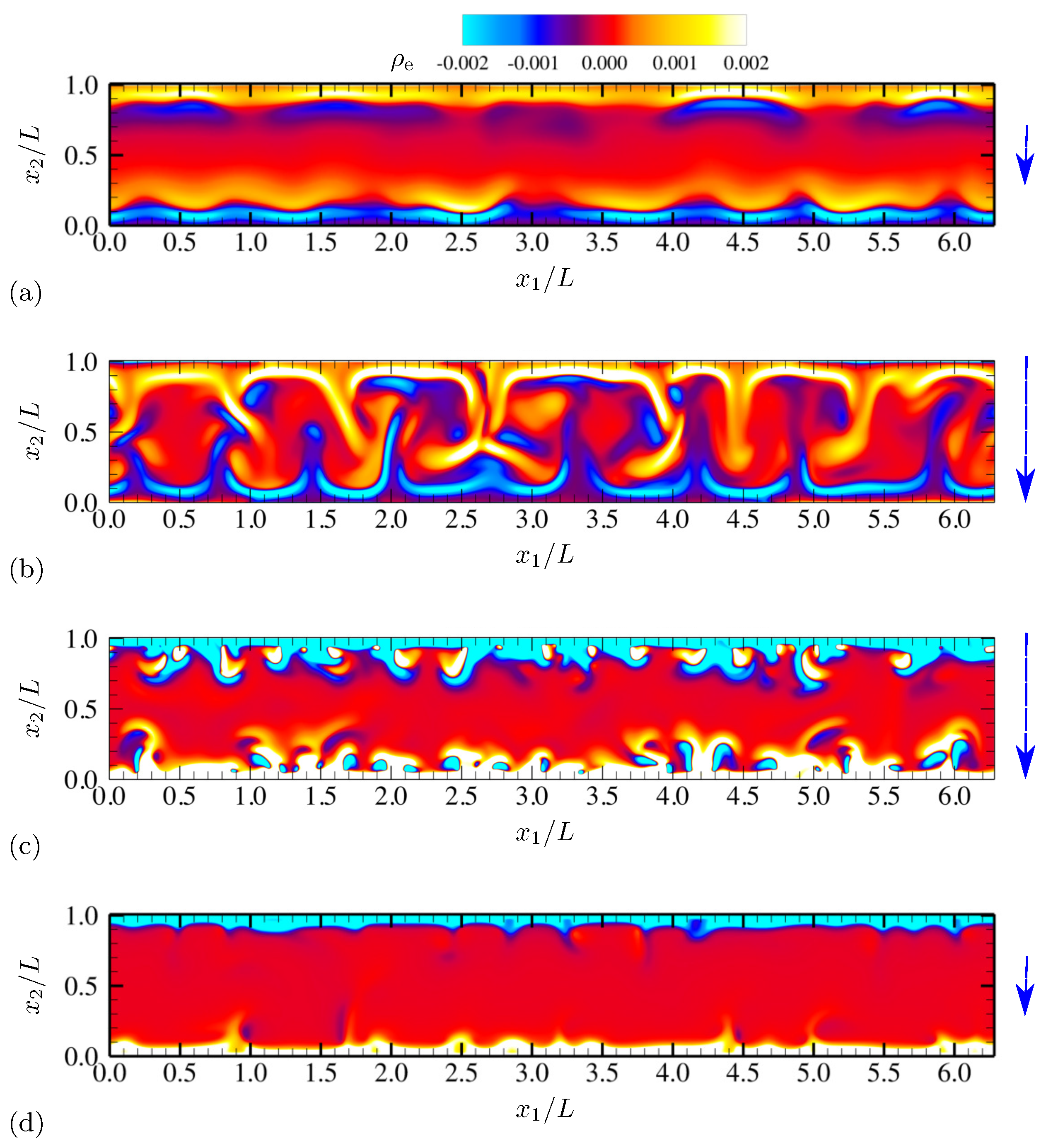
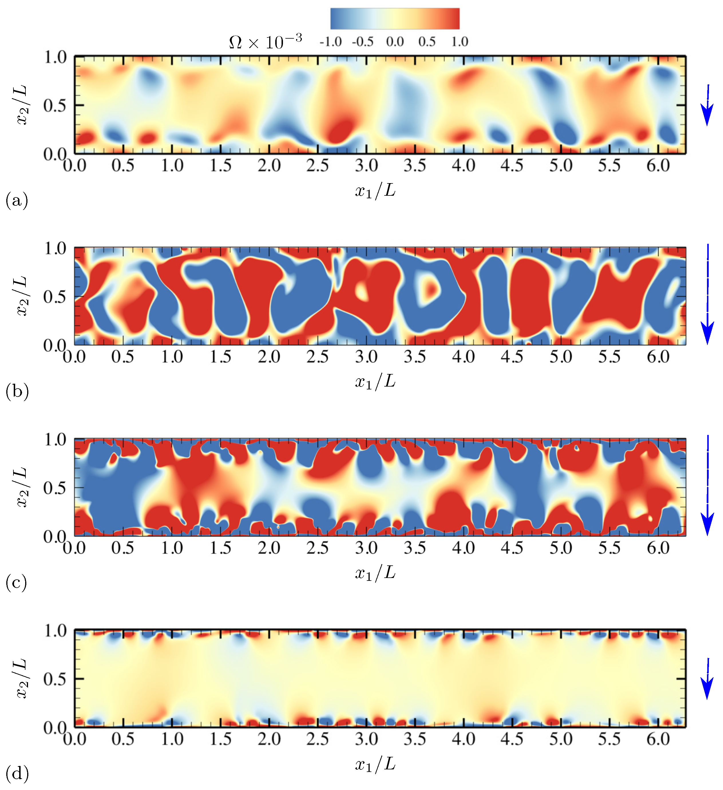
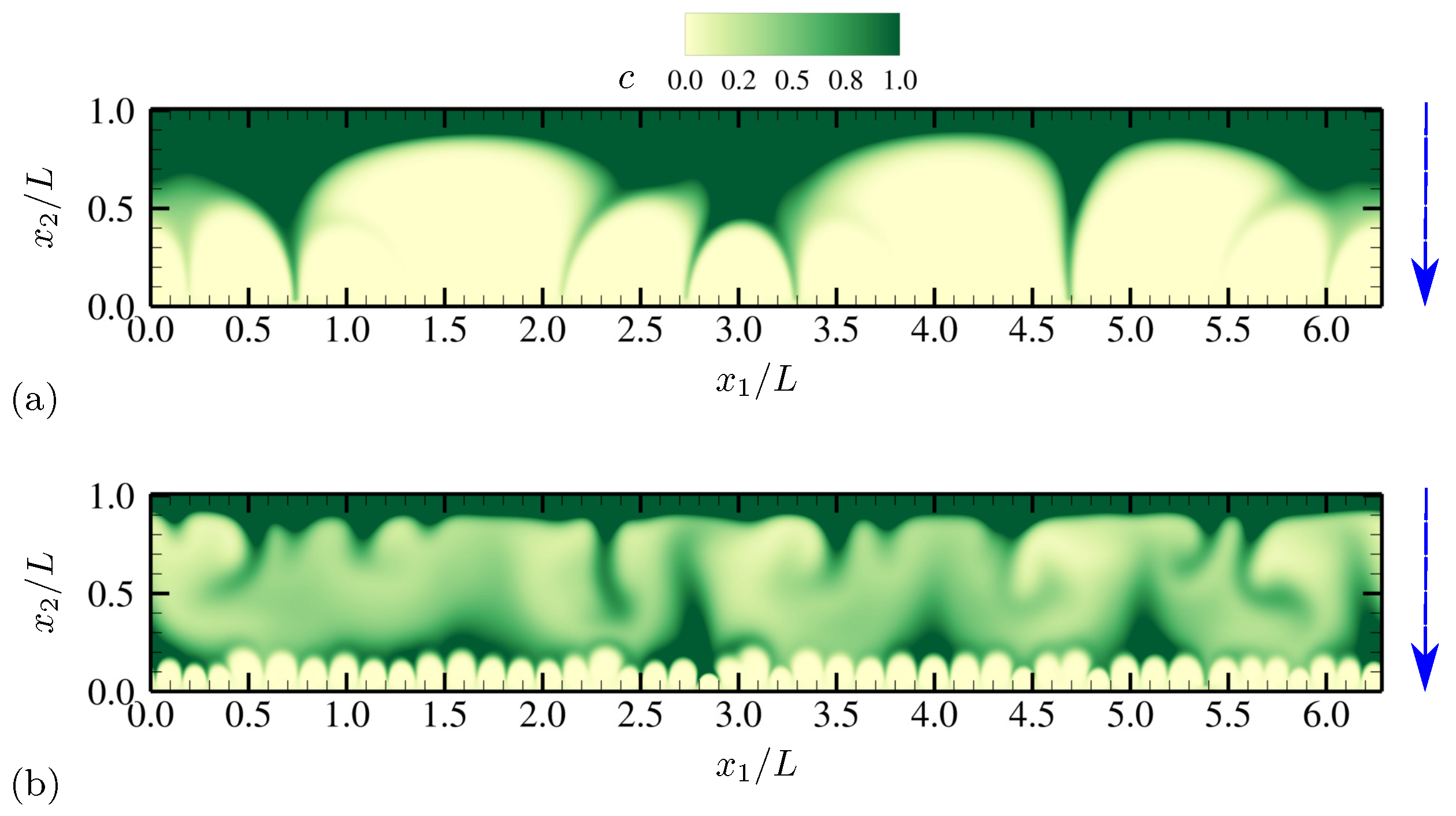
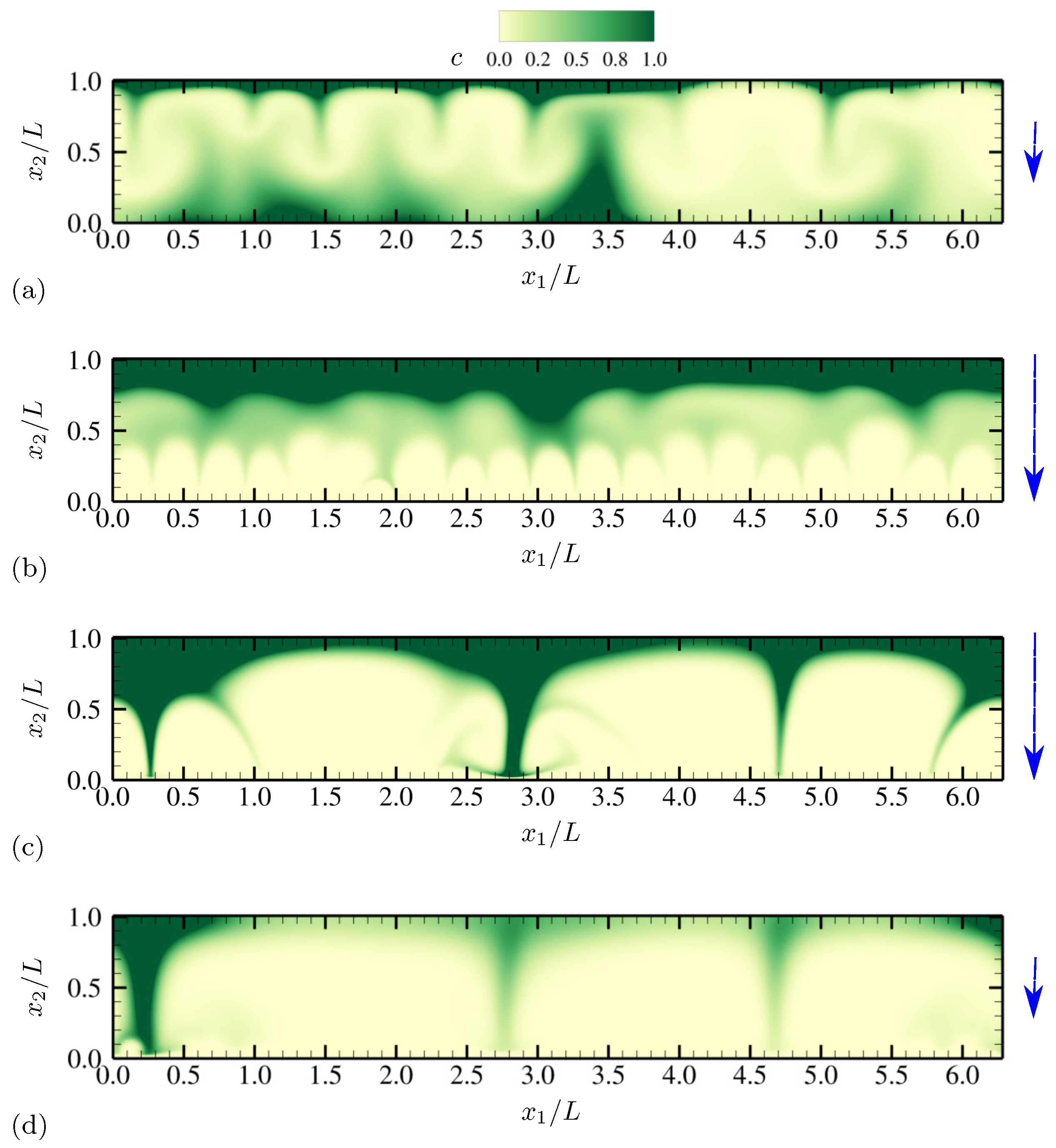
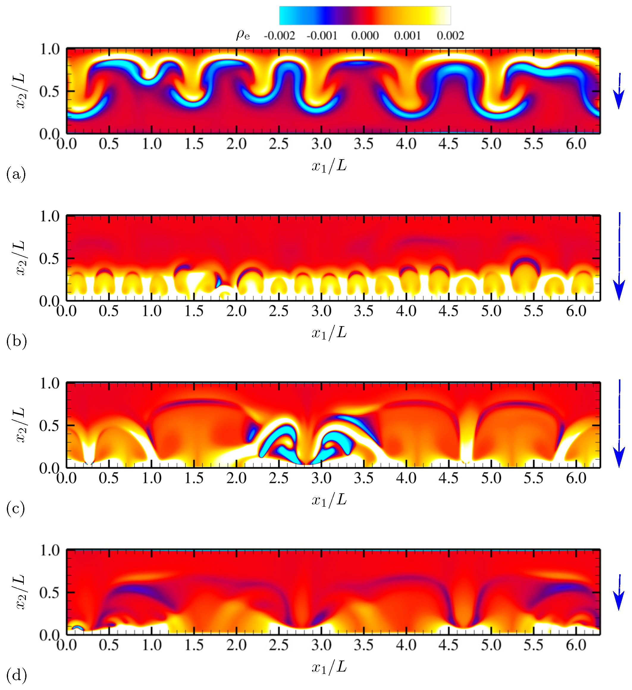
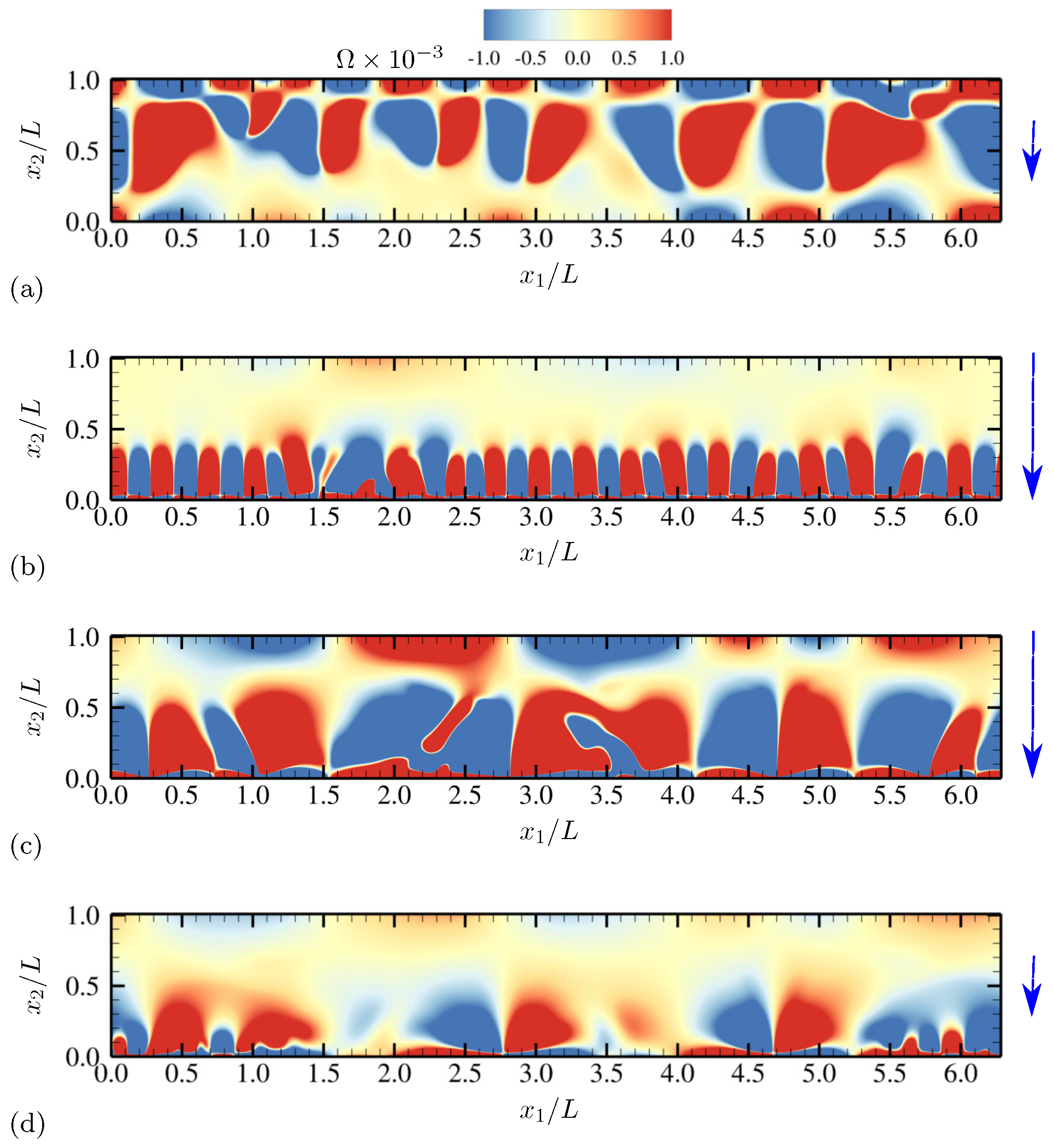
4.1.1. Evolution of Electrohydrodynamic Structures Under External AC Voltages
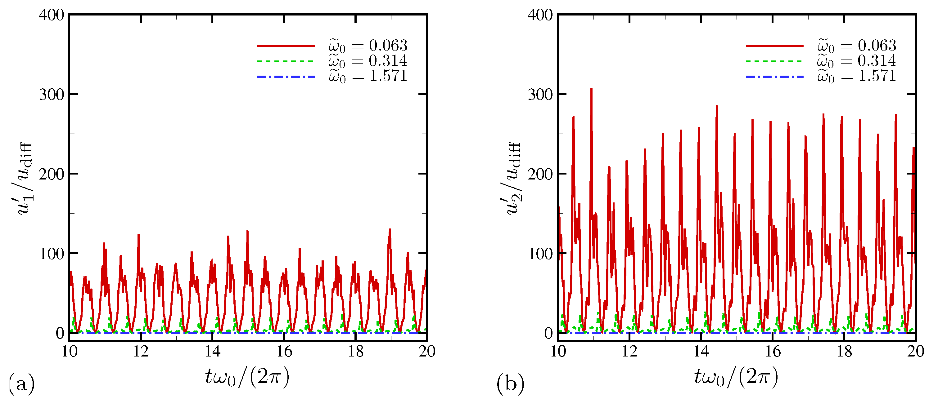
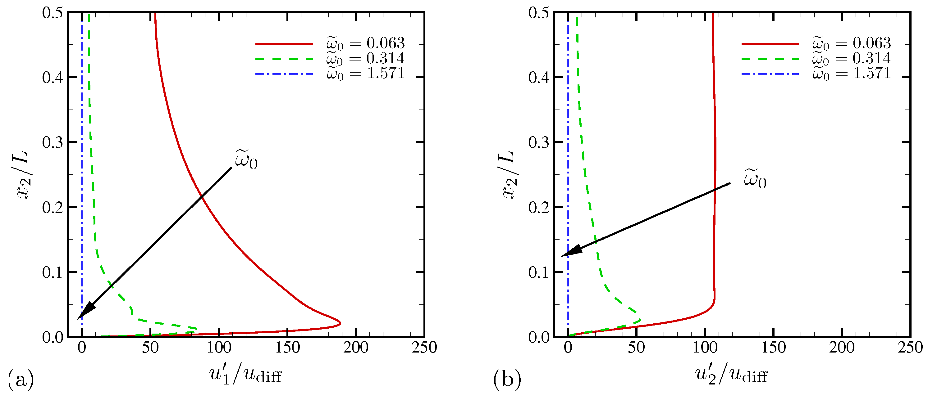
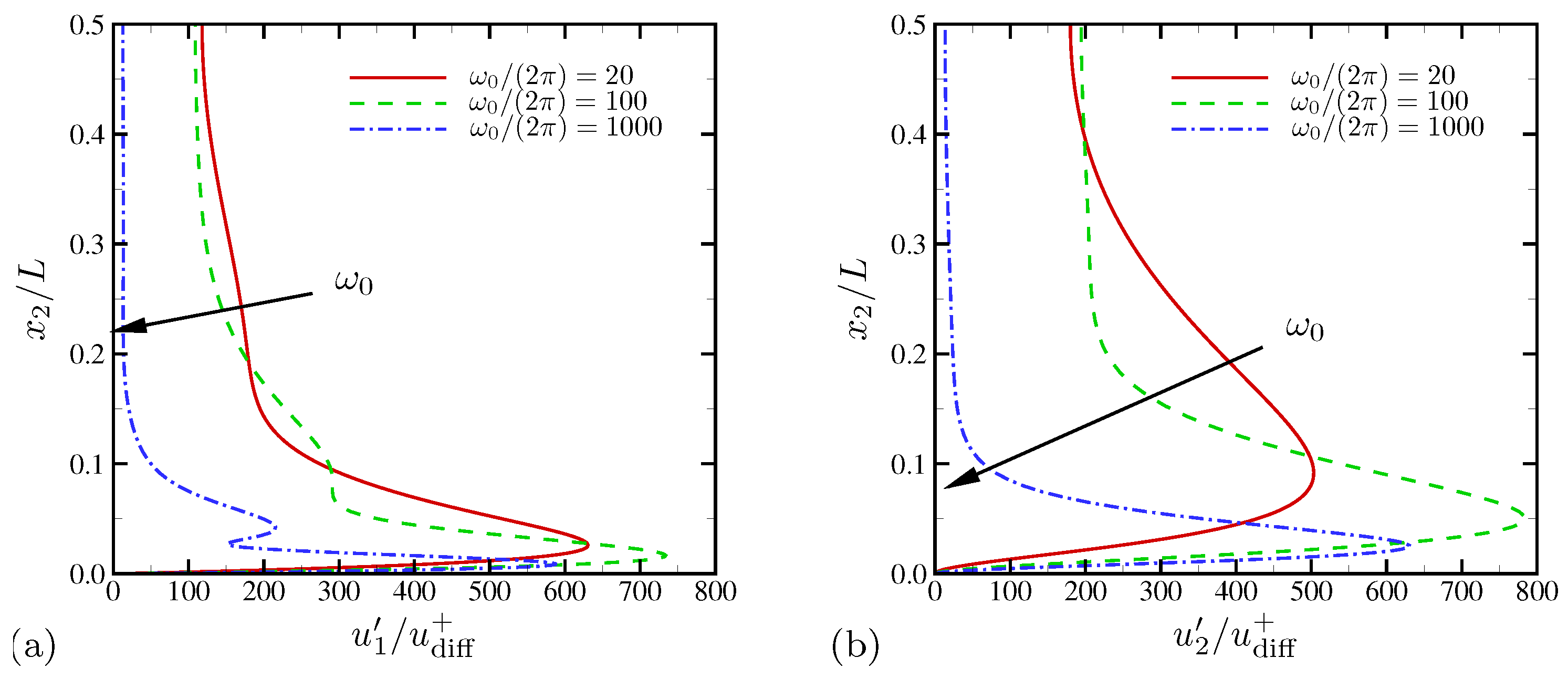
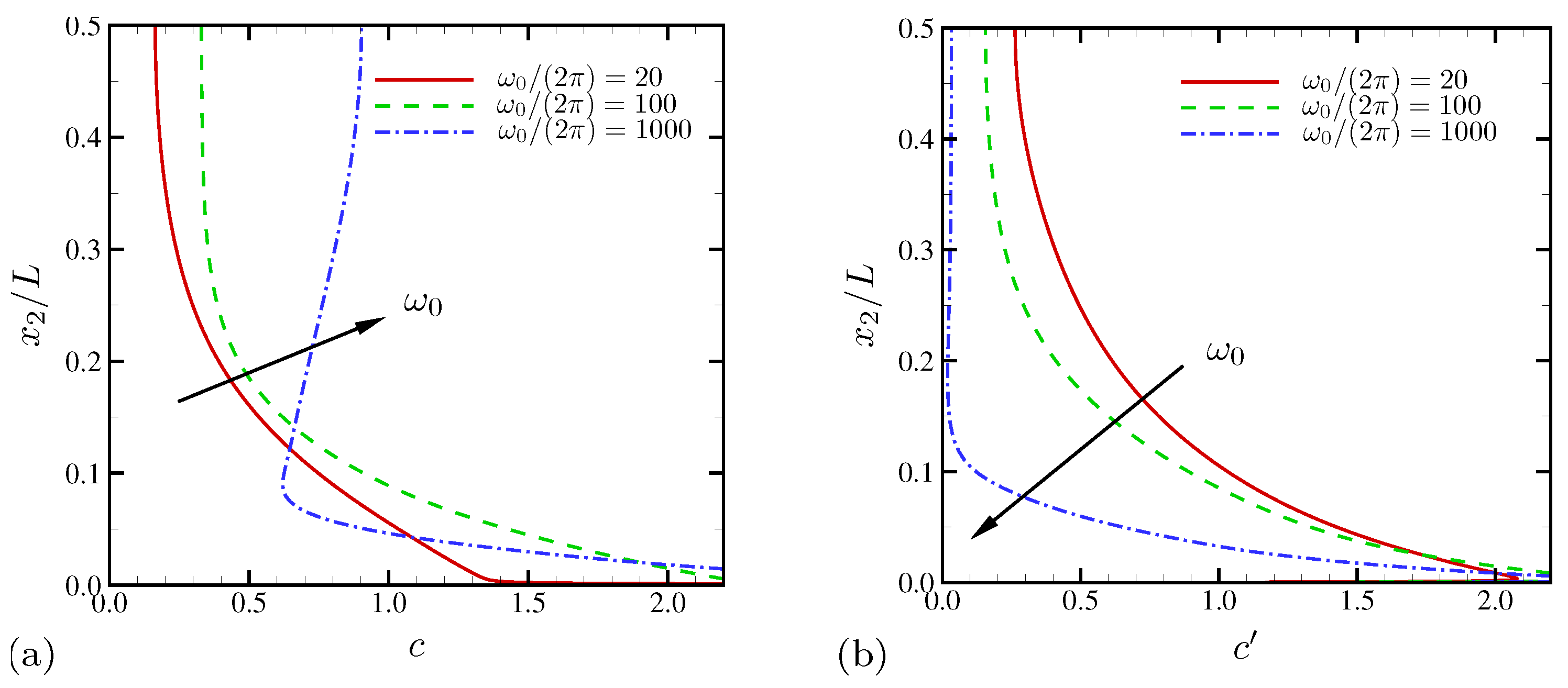
4.1.2. Statistics
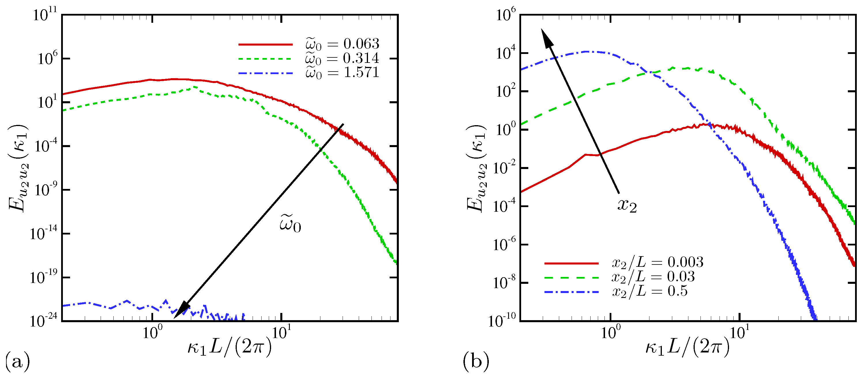
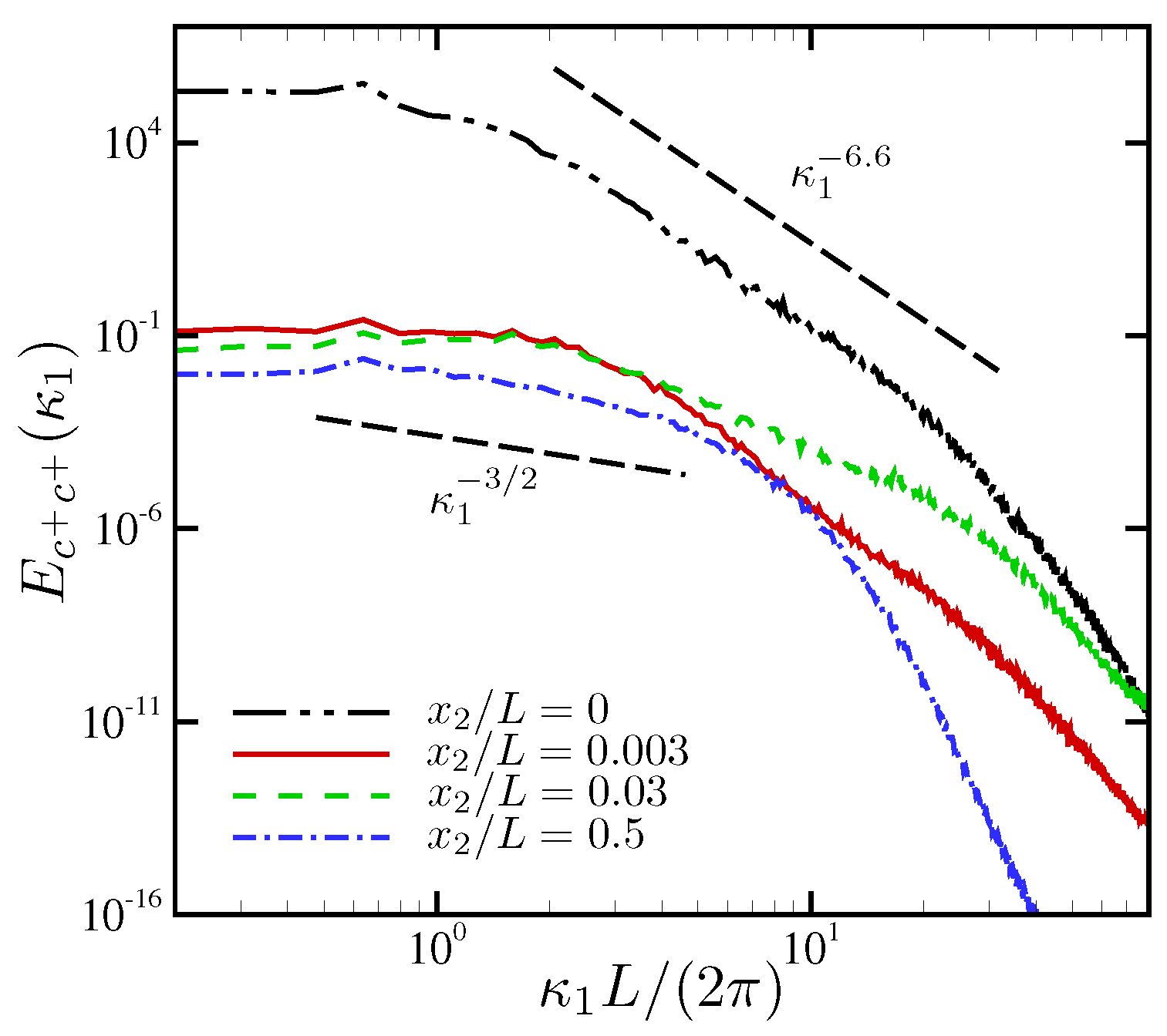
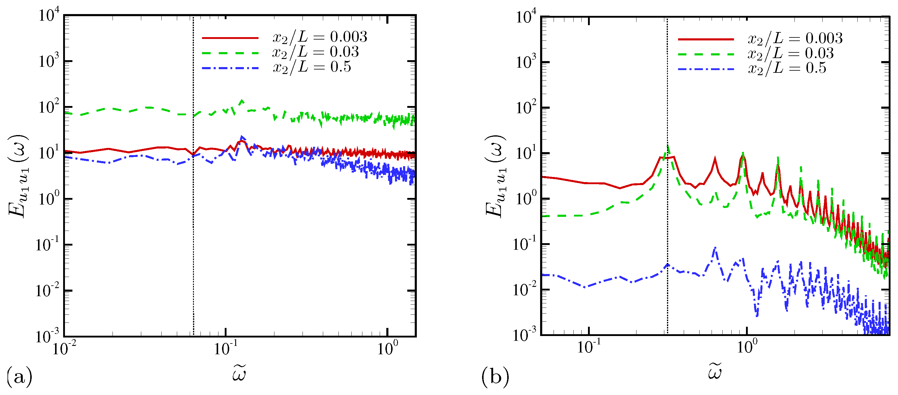
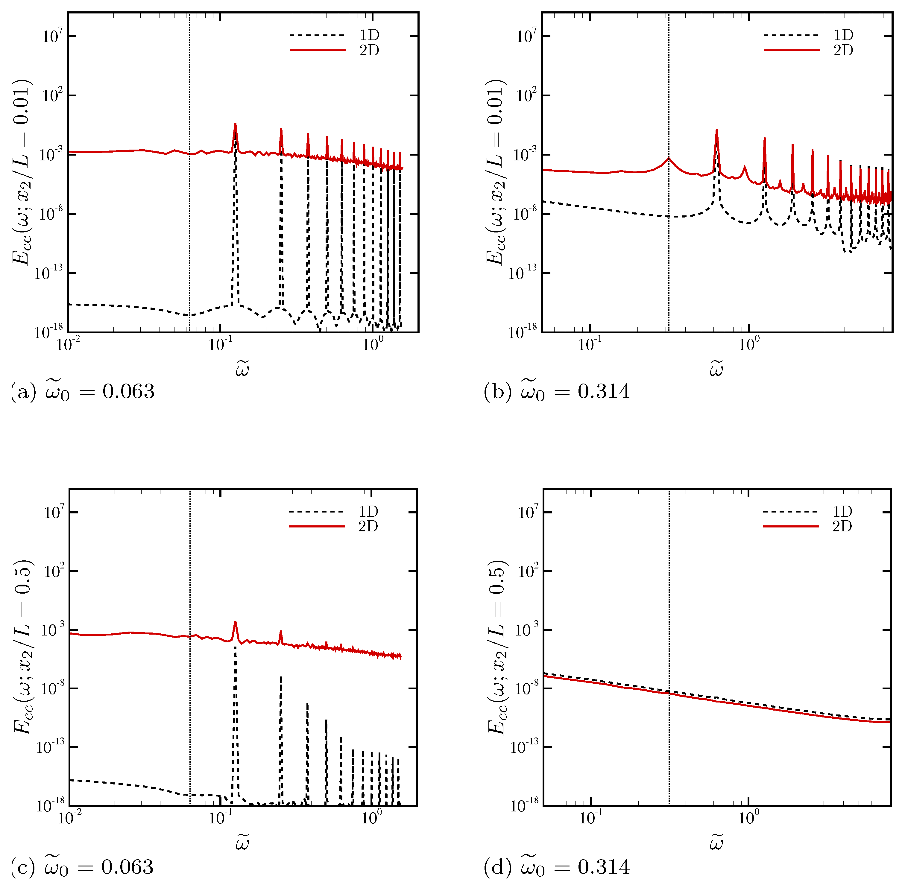
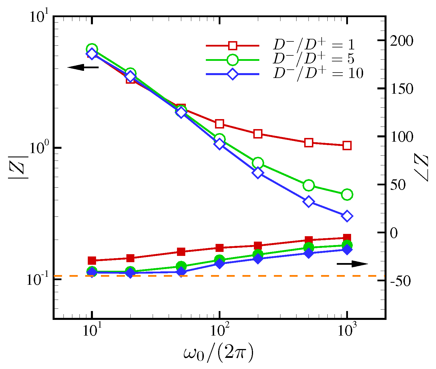
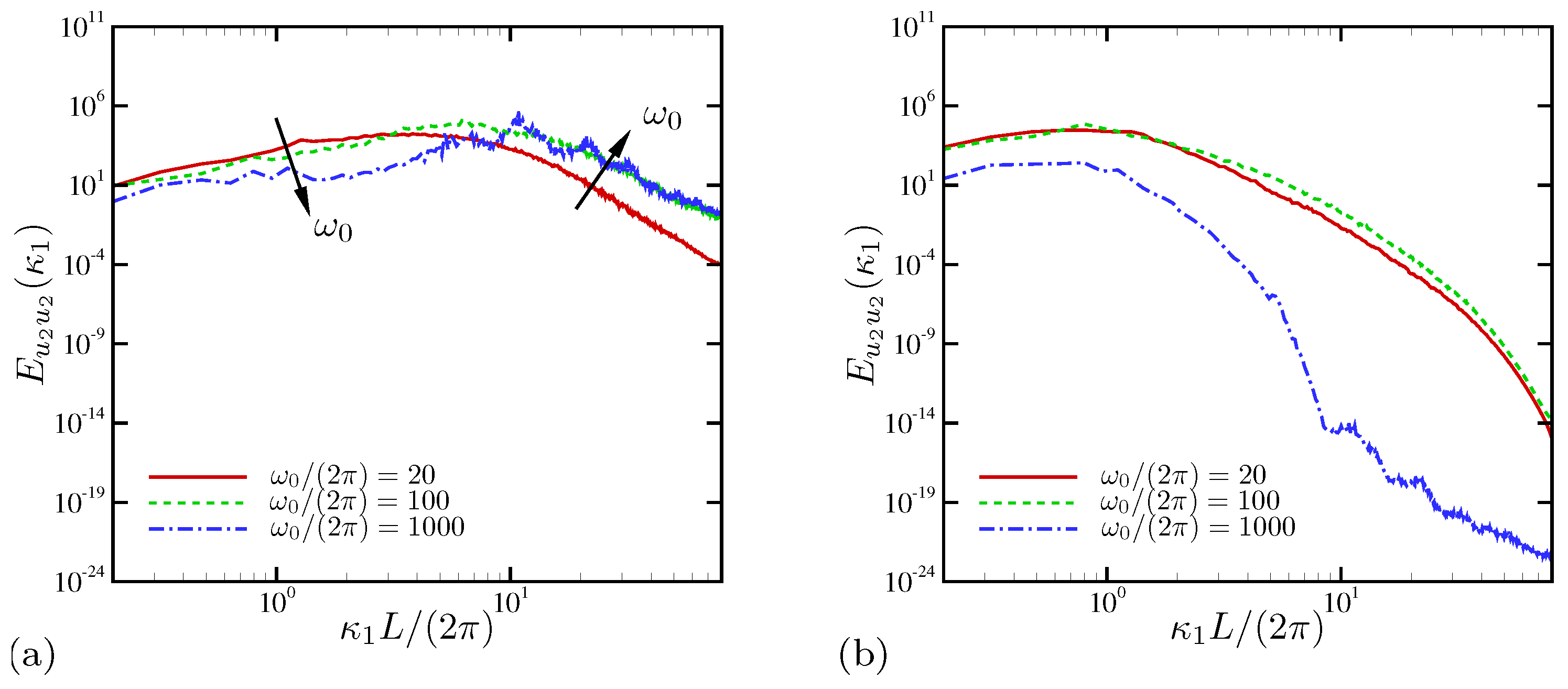
4.1.3. Spectral Analysis
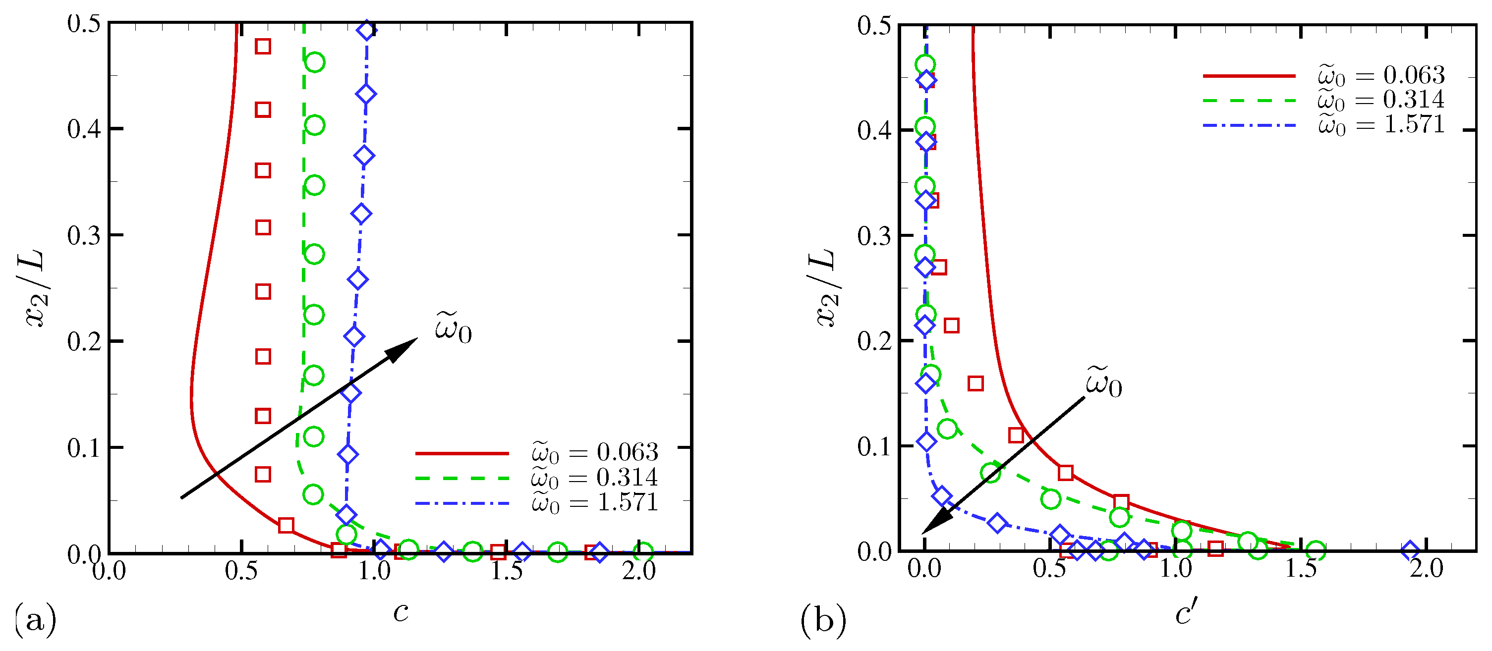
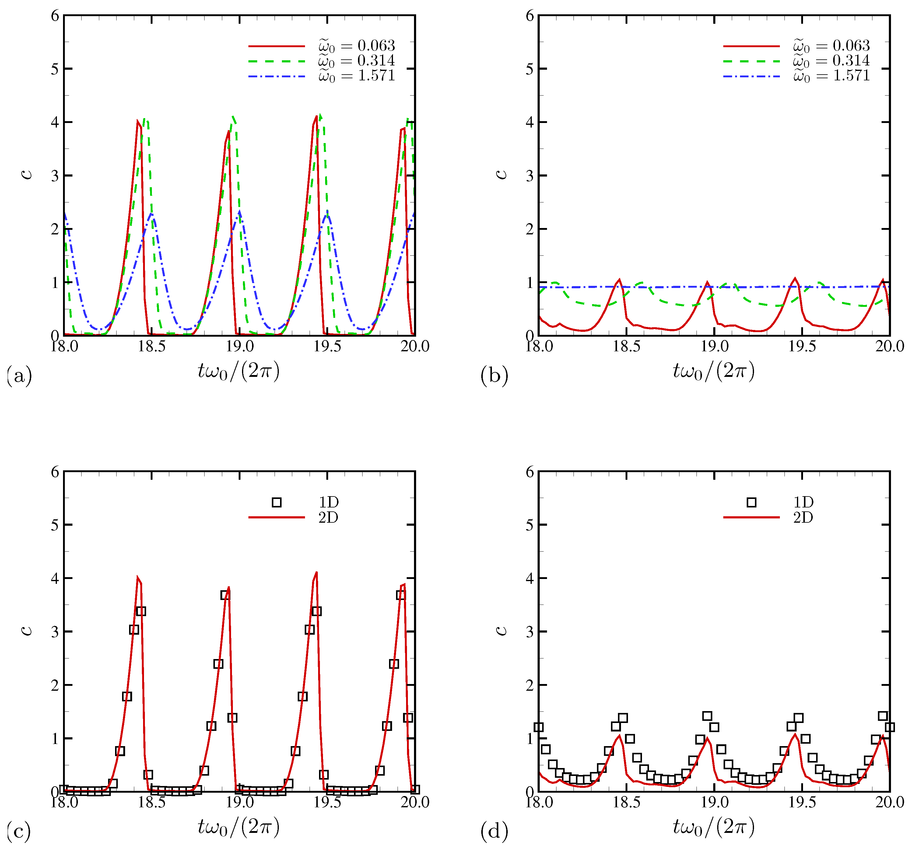
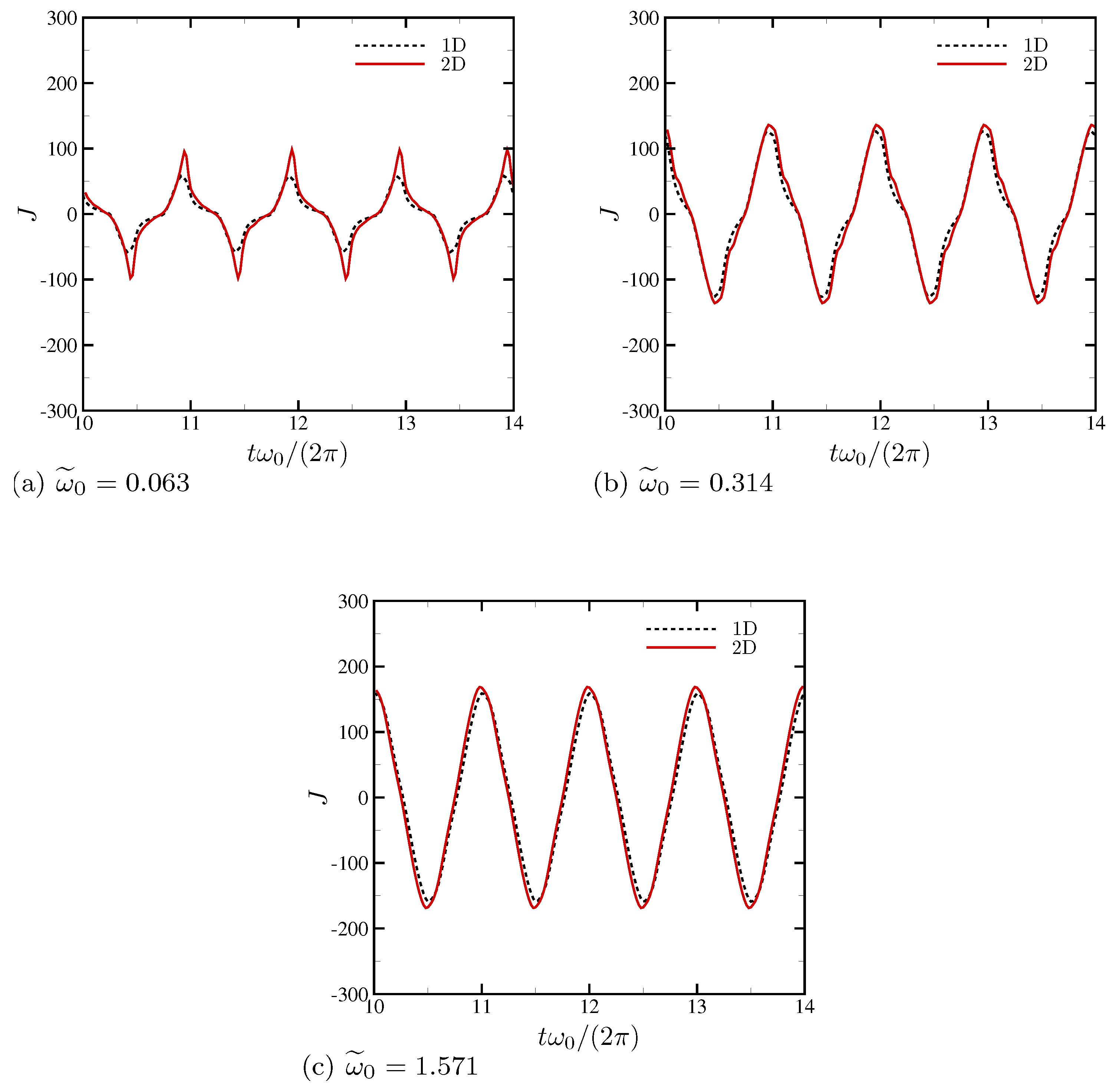
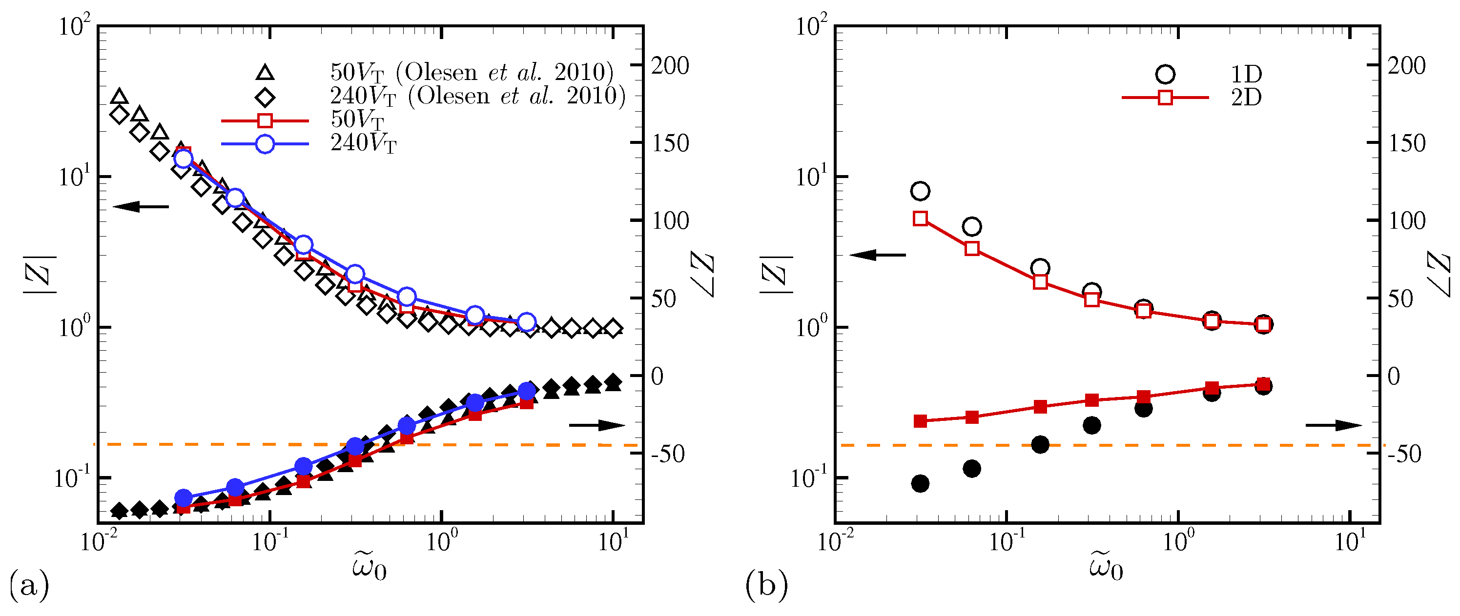
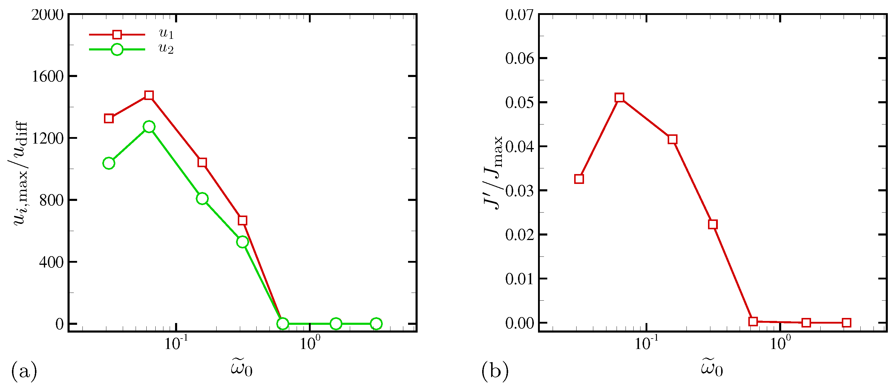
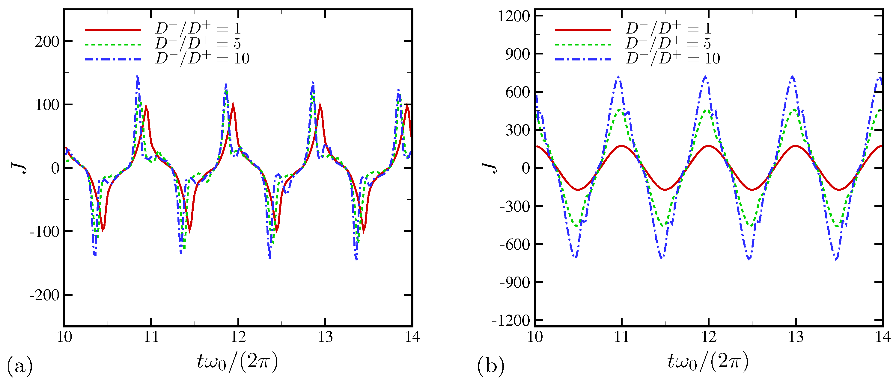
4.1.4. Electric Current and System-Level Responses
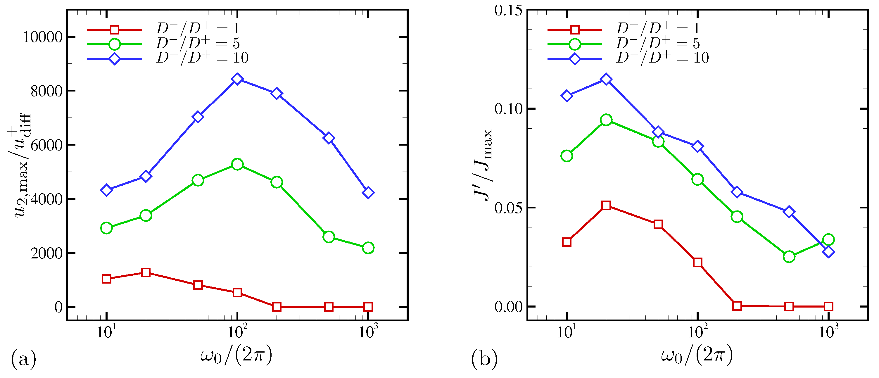
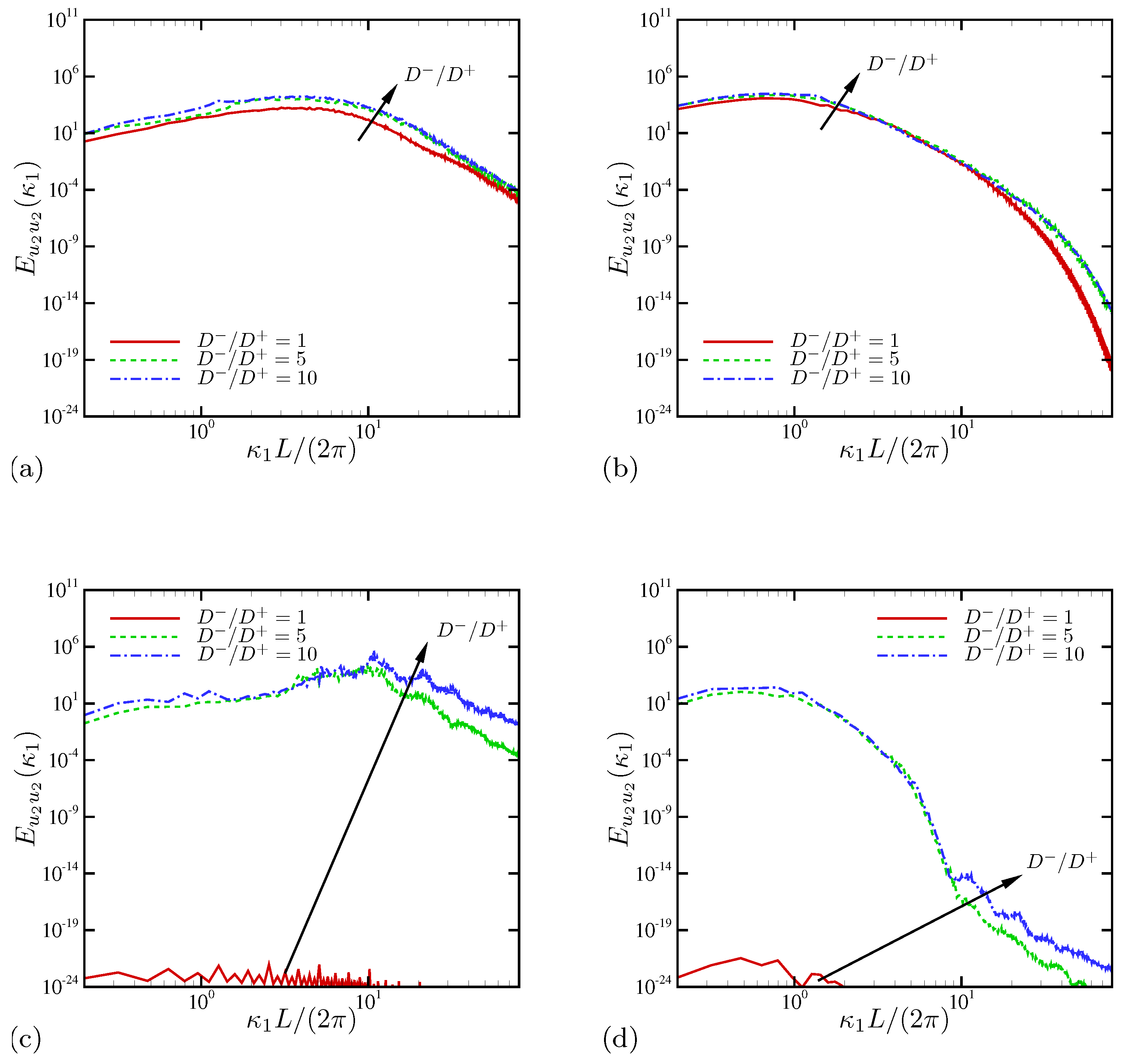
4.2. Effects of Ion Diffusivity on Electroconvective Instability
5. Conclusions and Discussions
Supplementary Materials
Author Contributions
Funding
Acknowledgments
Conflicts of Interest
References
- Rubinstein, I.; Zaltzman, B. Electro-osmotically induced convection at a permselective membrane. Phys. Rev. E 2000, 62, 2238. [Google Scholar] [CrossRef]
- Zaltzman, B.; Rubinstein, I. Electro-osmotic slip and electroconvective instability. J. Fluid Mech. 2007, 579, 173–226. [Google Scholar] [CrossRef]
- Rubinstein, I.; Staude, E.; Kedem, O. Role of the membrane surface in concentration polarization at ion-exchange membrane. Desalination 1988, 69, 101–114. [Google Scholar] [CrossRef]
- Rubinstein, S.M.; Manukyan, G.; Staicu, A.; Rubinstein, I.; Zaltzman, B.; Lammertink, R.G.; Mugele, F.; Wessling, M. Direct observation of a nonequilibrium electro-osmotic instability. Phys. Rev. Lett. 2008, 101, 236101. [Google Scholar] [CrossRef] [PubMed]
- De Valença, J.C.; Wagterveld, R.M.; Lammertink, R.G.H.; Tsai, P.A. Dynamics of microvortices induced by ion concentration polarization. Phys. Rev. E 2015, 92, 031003. [Google Scholar] [CrossRef] [PubMed]
- Levich, V.G. Physicochemical Hydrodynamics; Prentice-Hall: Englewood Cliffs, NJ, USA, 1962. [Google Scholar]
- Khair, A.S. Concentration polarization and second-kind electrokinetic instability at an ion-selective surface admitting normal flow. Phys. Fluids 2011, 23, 072003. [Google Scholar] [CrossRef]
- Druzgalski, C.L.; Andersen, M.B.; Mani, A. Direct numerical simulation of electroconvective instability and hydrodynamic chaos near an ion-selective surface. Phys. Fluids 2013, 25, 110804. [Google Scholar] [CrossRef]
- Demekhin, E.A.; Shelistov, V.S.; Polyanskikh, S.V. Linear and nonlinear evolution and diffusion layer selection in electrokinetic instability. Phys. Rev. E 2011, 84, 036318. [Google Scholar] [CrossRef] [PubMed]
- Demekhin, E.A.; Nikitin, N.V.; Shelistov, V.S. Direct numerical simulation of electrokinetic instability and transition to chaotic motion. Phys. Fluids 2013, 25, 122001. [Google Scholar] [CrossRef]
- Pham, V.S.; Li, Z.; Lim, K.M.; White, J.K.; Han, J. Direct numerical simulation of electroconvective instability and hysteretic current-voltage response of a permselective membrane. Phys. Rev. E 2012, 86, 046310. [Google Scholar] [CrossRef] [PubMed]
- Druzgalski, C.; Mani, A. Statistical analysis of electroconvection near an ion-selective membrane in the highly chaotic regime. Phys. Rev. Fluids 2016, 1, 073601. [Google Scholar] [CrossRef]
- Wang, K.M.; Mani, A. Scale dependence of flow structures in electroconvection. Proc. Natl. Acad. Sci. USA 2018. submitted. [Google Scholar]
- Karatay, E.; Druzgalski, C.L.; Mani, A. Simulation of chaotic electrokinetic transport: Performance of commercial software versus custom-built direct numerical simulation codes. J. Colloid Interf. Sci. 2015, 446, 67–76. [Google Scholar] [CrossRef] [PubMed]
- Chang, H.C.; Yossifon, G.; Demekhin, E.A. Nanoscale electrokinetics and microvortices: How microhydrodynamics affects nanofluidic ion flux. Annu. Rev. Fluid Mech. 2012, 44, 401–426. [Google Scholar] [CrossRef]
- Nikonenko, V.V.; Kovalenko, A.V.; Urtenov, M.K.; Pismenskaya, N.D.; Han, J.; Sistat, P.; Pourcelly, G. Desalination at overlimiting currents: State-of-the-art and perspectives. Desalination 2014, 342, 85–106. [Google Scholar] [CrossRef]
- Nikonenko, V.V.; Vasil’eva, V.I.; Akberova, E.M.; Uzdenova, A.M.; Urtenov, M.K.; Kovalenko, A.V.; Pismenskaya, N.P.; Mareev, S.A.; Pourcelly, G. Competition between diffusion and electroconvection at an ion-selective surface in intensive current regimes. Adv. Colloid Interface 2016, 235, 233–246. [Google Scholar] [CrossRef] [PubMed]
- Nikonenko, V.V.; Mareev, S.A.; Pis’menskaya, N.D.; Uzdenova, A.M.; Kovalenko, A.V.; Urtenov, M.K.; Pourcelly, G. Effect of electroconvection and its use in intensifying the mass transfer in electrodialysis. Russ. J. Electrochem. 2017, 53, 1122–1144. [Google Scholar] [CrossRef]
- Chu, K.T.; Bazant, M.Z. Electrochemical thin films at and above the classical limiting current. SIAM J. Appl. Math. 2005, 65, 1485–1505. [Google Scholar] [CrossRef]
- Davidson, S.M.; Andersen, M.B.; Mani, A. Chaotic induced-charge electro-osmosis. Phys. Rev. Lett. 2014, 112, 128302. [Google Scholar] [CrossRef] [PubMed]
- Im, S.; Do, H.; Cappelli, M.A. Dielectric barrier discharge control of a turbulent boundary layer in a supersonic flow. Appl. Phys. Lett. 2010, 97, 041503. [Google Scholar] [CrossRef]
- Bazant, M.Z.; Squires, T.M. Induced-charge electrokinetic phenomena: theory and microfluidic applications. Phys. Rev. Lett. 2004, 92, 066101. [Google Scholar] [CrossRef] [PubMed]
- Squires, T.M.; Bazant, M.Z. Induced-charge electro-osmosis. J. Fluid Mech. 2004, 509, 217–252. [Google Scholar] [CrossRef]
- Stout, R.F.; Khair, A.S. Moderately nonlinear diffuse-charge dynamics under an ac voltage. Phys. Rev. E 2015, 92, 032305. [Google Scholar] [CrossRef] [PubMed]
- Dibua, O.L.; Ramsurrun, S.; Mani, A.; Pruitt, B.L.; Iaccarino, G. Hierarchy of models for electrostatic comb-drive actuators in electrolytes. J. Micromech. Microeng. 2018, 28, 125013. [Google Scholar] [CrossRef]
- Bazant, M.Z.; Thornton, K.; Ajdari, A. Diffuse-charge dynamics in electrochemical systems. Phys. Rev. E 2004, 70, 021506. [Google Scholar] [CrossRef] [PubMed]
- Suh, Y.K.; Kang, S. Asymptotic analysis of ion transport in a nonlinear regime around polarized electrodes under ac. Phys. Rev. E 2008, 77, 031504. [Google Scholar] [CrossRef] [PubMed]
- Olesen, L.H.; Bazant, M.Z.; Bruus, H. Strongly nonlinear dynamics of electrolytes in large ac voltages. Phys. Rev. E 2010, 82, 011501. [Google Scholar] [CrossRef] [PubMed]
- Schnitzer, O.; Yariv, E. Nonlinear oscillations in an electrolyte solution under ac voltage. Phys. Rev. E 2014, 89, 032302. [Google Scholar] [CrossRef] [PubMed]
- Davidson, S.M.; Wessling, M.; Mani, A. On the dynamical regimes of pattern-accelerated electroconvection. Sci. Rep. 2016, 6, 22505. [Google Scholar] [CrossRef] [PubMed]
- Kilic, M.S.; Bazant, M.Z.; Ajdari, A. Steric effects in the dynamics of electrolytes at large applied voltages. II. Modified Poisson–Nernst–Planck equations. Phys. Rev. E 2007, 75, 021503. [Google Scholar] [CrossRef] [PubMed]
- Gillespie, D. A review of steric interactions of ions: Why some theories succeed and others fail to account for ion size. Microfluid. Nanofluid. 2015, 18, 717–738. [Google Scholar] [CrossRef]
- Davidson, S.M. A Comprehensive Investigation of Electroconvection in Canonical Electrochemical Environments. Ph.D. Thesis, Stanford University, Stanford, CA, USA, 2017. [Google Scholar]
- Piomelli, U. Wall-layer models for large-eddy simulations. Prog. Aerospace Sci. 2008, 44, 437–446. [Google Scholar] [CrossRef]


| Dimensionless Parameters | Descriptions |
|---|---|
| electrohydrodynamic coupling constant | |
| nondimensional Debye screening length | |
| Schmidt number | |
| nondimensional maximum voltage | |
| nondimensional oscillation frequency | |
| ratio of ionic diffusivities |
© 2019 by the authors. Licensee MDPI, Basel, Switzerland. This article is an open access article distributed under the terms and conditions of the Creative Commons Attribution (CC BY) license (http://creativecommons.org/licenses/by/4.0/).
Share and Cite
Kim, J.; Davidson, S.; Mani, A. Characterization of Chaotic Electroconvection near Flat Inert Electrodes under Oscillatory Voltages. Micromachines 2019, 10, 161. https://doi.org/10.3390/mi10030161
Kim J, Davidson S, Mani A. Characterization of Chaotic Electroconvection near Flat Inert Electrodes under Oscillatory Voltages. Micromachines. 2019; 10(3):161. https://doi.org/10.3390/mi10030161
Chicago/Turabian StyleKim, Jeonglae, Scott Davidson, and Ali Mani. 2019. "Characterization of Chaotic Electroconvection near Flat Inert Electrodes under Oscillatory Voltages" Micromachines 10, no. 3: 161. https://doi.org/10.3390/mi10030161
APA StyleKim, J., Davidson, S., & Mani, A. (2019). Characterization of Chaotic Electroconvection near Flat Inert Electrodes under Oscillatory Voltages. Micromachines, 10(3), 161. https://doi.org/10.3390/mi10030161