
Muscle Biomarkers in Colorectal Cancer Outpatients: Agreement Between Computed Tomography, Bioelectrical Impedance Analysis, and Nutritional Ultrasound
 , and
, and
Abstract

1. Introduction
- Can all techniques detect similar patterns in body composition in the study sample?
- Are a reference (CT) and bedside techniques (BIA, US) interchangeable using current regression equations for MM or FFM in the study sample?
- How do current operational definitions of muscle atrophy, myosteatosis, and sarcopenia agree in the study sample?
2. Materials and Methods
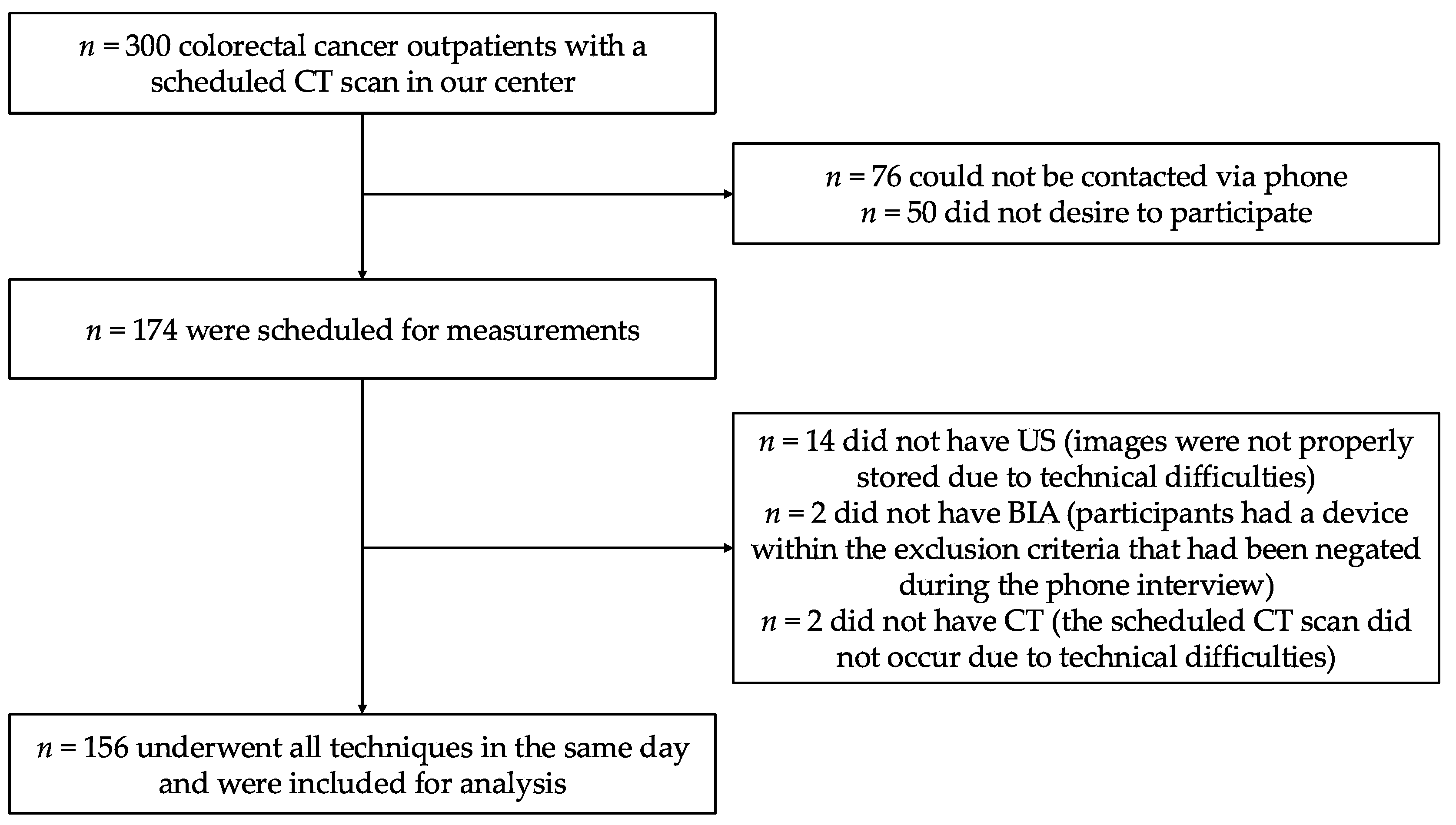
2.1. Study Design
- Colorectal cancer outpatients over 50 years of age;
- Under active surveillance by the Oncology Department;
- With a programmed abdominal CT scan;
- Eastern Cooperative Oncology Group (ECOG) performance status of 0 to 3.
- ECOG 4-5;
- Terminal illness;
- Presence of a pacemaker, implantable cardioverter defibrillator, or intrathecal pain pump;
- Skin lesions or severe adhesive dermatitis that contraindicated electrode placement in the required areas for BIA;
- Severe cognitive impairment;
- Medical conditions that may artifact measurements at the discretion of the researcher (stroke with right residual hemiplegia, amyotrophic lateral sclerosis, or muscular dystrophy that may affect BIA and US; symptomatic rheumatoid arthritis or gouty arthritis of hand and wrist that may affect HGS);
- Unable to perform an informed consent or no desire for participation.
2.2. Procedures
2.2.1. Computed Tomography (CT) Scan Segmentation
2.2.2. Bioelectrical Impedance Analysis (BIA)
2.2.3. Nutritional Ultrasound® (US)
2.2.4. Anthropometry Protocol
2.2.5. Handgrip Strength (HGS) Measurements
2.2.6. Clinical Variables and Cancer Staging
2.2.7. Operative Definitions of Muscle Atrophy, Myosteatosis, Dynapenia, Sarcopenia, Malnutrition, and Obesity
2.3. Data Quality
2.4. Statistical Analysis
3. Results
3.1. Description of the Study Sample
3.2. Muscle Biomarkers
3.2.1. General Description
3.2.2. CT Muscle Biomarkers
3.2.3. BIA Biomarkers
3.2.4. US Biomarkers and Handgrip Strength
3.3. Muscle Biomarkers: Intra and Inter-Technique Correlation Matrices
3.3.1. Matrix 1: CT, BIA, and HGS
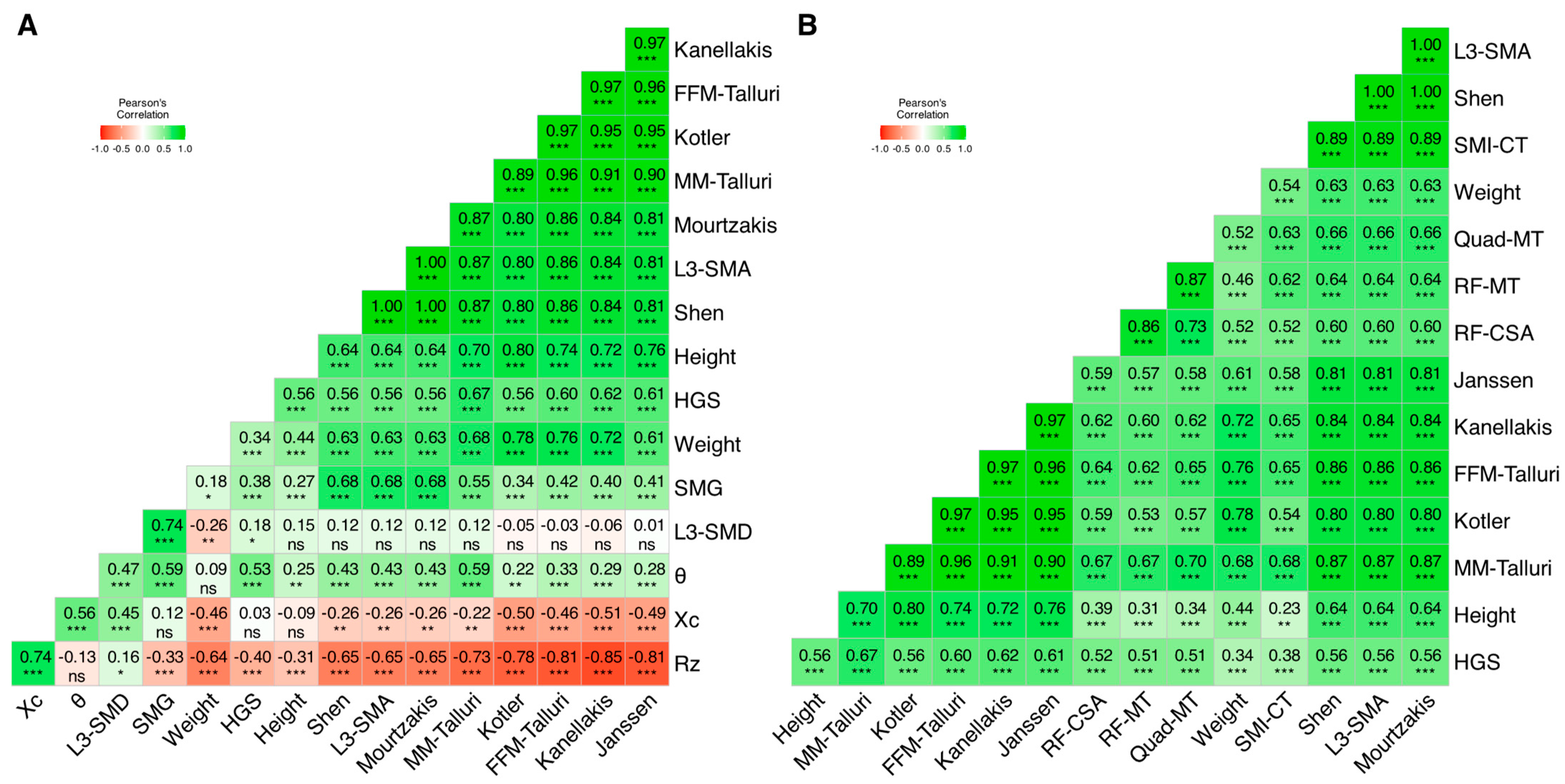
- Rz had moderate inverse correlations with L3-SMA (r = −0.65), weight (r = −0.65), and HGS (r = −0.40), as well as a moderate direct correlation with Xc (r = 0.74).
- Conversely, Xc had moderate direct correlations with θ (r = 0.56), and L3-SMD (r = 0.45).
- θ had moderate direct correlations with SMG (r = 0.59), HGS (r = 0.53), L3-SMD (r = 0.47), and L3-SMA (r = 0.43).
- Maximum handgrip strength showed a moderate correlation with these parameters, being the highest for MM Talluri (r = 0.67).
3.3.2. Matrix 2: CT, US, and HGS
3.4. Muscle Biomarkers: Agreement
3.4.1. Agreement Between CT and BIA
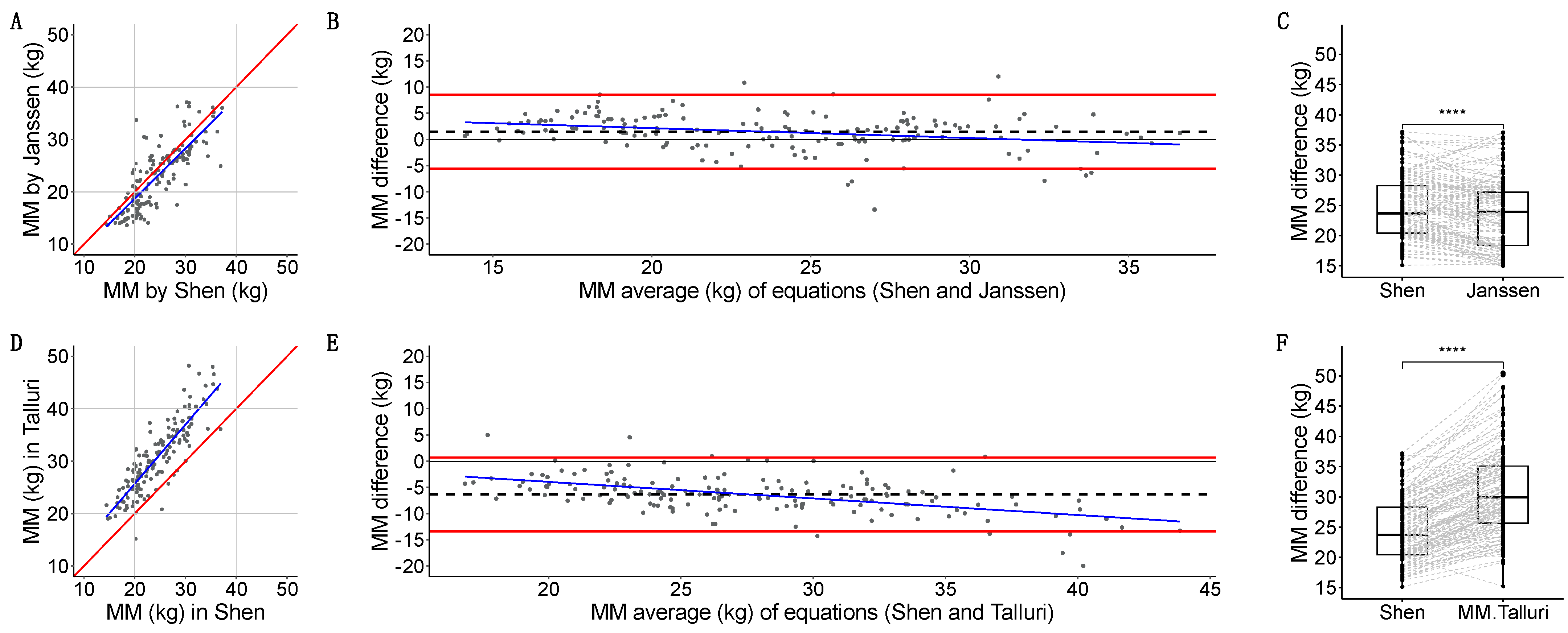
- Janssen-estimated MM [34] had a strong linear relation with Shen [2] (r = 0.809, p < 2.2 × 10⁻¹⁶) (Figure 6A). Quantitative agreement was poor (ρ = 0.772, 95%CI: 0.705, 0.825). Janssen underestimated MM with a 1.5 (3.6) kg systematic bias, a minimal dose-dependent bias, (−5.6, 8.6) kg LoA, and 9/156 (5.7%) measurements outside the LoA (Figure 6B). Grouped measurements were significantly different (23.3 vs. 23.6 kg, p = 3.609 × 10⁻⁸) (Figure 6C).
- Talluri-estimated MM had a strong linear relation with Shen [2] (r = 0.865, p < 2.2 × 10⁻¹⁶) (Figure 6D). Quantitative agreement was poor (ρ = 0.538, 95%CI: 0.467, 0.603). Talluri overestimated MM with a −6.4 (3.6) kg systematic bias, a dose-dependent bias, (−13–41, 0.688) kg LoA, and 9/156 (5.7%) measurements outside the LoA (Figure 6E). Grouped measurements were significantly different (29.9 vs. 23.6 kg, p < 2.2 × 10⁻¹⁶) (Figure 6F).
- Kanellakis-estimated FFM [36] had a strong linear relation with Mourtzakis [3] (r = 0.836, p < 2.2 × 10⁻¹⁶) (Figure 7A). Quantitative agreement was poor (ρ = 0.468, 95%CI: 0.396, 0.534). Kanellakis underestimated FFM with a 12.5 (6.7) kg systematic bias, a linear regression model compatible with a dose-dependent bias, (−0.6, 2.6) kg LoA, and 9/156 (5.7%) measurements outside the LoA (Figure 7B). Grouped measurements were significantly different (32.6 vs. 42.4 kg, p < 2.2 × 10⁻¹⁶) (Figure 7C).
- Kotler-estimated FFM [37] had a strong linear relation with Mourtzakis [3] (r = 0.802, p < 2.2 × 10⁻¹⁶) (Figure 7D). Quantitative agreement was poor (ρ = 0.718, 95%CI: 0.643, 0.780). Kotler overestimated FFM with a −4.3 (5.7) kg systematic bias, no dose-dependent bias, (−15.4, 6.8) kg LoA, and 9/156 (5.7%) measurements outside the LoA (Figure 7E). Grouped measurements were significantly different (47.7 vs. 42.4 kg, p = 3.464 × 10⁻¹⁶) (Figure 7F).
- Talluri-estimated FFM had a strong linear relation with Mourtzakis [3] (r = 0.857, p < 2.2 × 10⁻¹⁶) (Figure 7G). Quantitative agreement was poor (ρ = 0.666, 95CI%: 0.595, 0.728). Talluri overestimated FFM with a −6.9 (5.0) kg systematic bias, no dose-dependent bias, (−16.7, 2.9) kg LoA, and 11/156 (7.0%) measurements outside the LoA (Figure 7H). Grouped measurements were significantly different (49.9 vs. 42.4 kg, p < 2.2 × 10⁻¹⁶) (Figure 7I).
3.4.2. Agreement Between CT and US
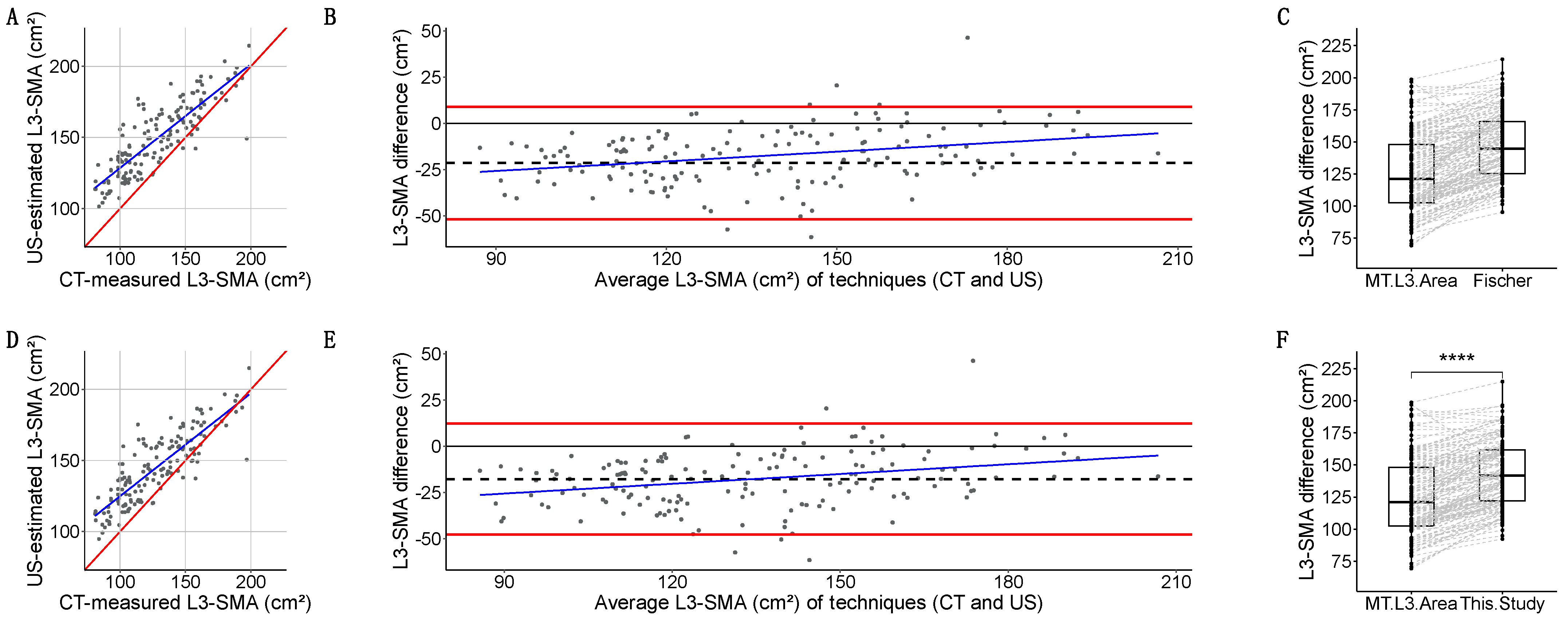
- Fischer-estimated L3-SMA [38] had a strong linear relation with L3-SMA (r = 0.849, p < 2.2 × 10⁻¹⁶) (Figure 8A). Quantitative agreement was poor (ρ = 0.642, 95%CI: 0.568, 0.705). Fischer overestimated L3-SMA with a −21.5 (15.2) cm2 bias, a dose-dependent bias in linear regression, and (−51.9, 8.9) kg LoA (Figure 8B). Grouped measurements were significantly different: 144.6 (40.7) vs. 121.2 (45.5) cm2 (p < 2.2 × 10⁻¹⁶) (Figure 8C).
- Our new equation had a strong linear relation with L3-SMA (r = 0.854, p < 2.2 × 10⁻¹⁶) (Figure 8D). Quantitative agreement was poor (ρ = 0.696, 95%CI: 0.626, 0.755). Our equation overestimated L3-SMA with a −17.6 (15.3) cm2 bias, a dose-dependent bias in linear regression, and (−47.6, 12.3) kg LoA (Figure 8E). Grouped measurements were significantly different: 141.7 (39.6) vs. 121.2 (45.5) cm2 (p < 2.2 × 10⁻¹⁶) (Figure 8F).
3.5. Impact of Techniques and Definitions on the Clinical Diagnosis of Muscle Atrophy
3.5.1. Intra-Technique (Between Definitions) Agreement
3.5.2. Inter-Technique Agreement
4. Discussion
5. Conclusions
Supplementary Materials
Author Contributions
Funding
Institutional Review Board Statement
Informed Consent Statement
Data Availability Statement
Conflicts of Interest
Appendix A

| Men | Women | |||||||
|---|---|---|---|---|---|---|---|---|
| BMI (kg/m2) | BMI (kg/m2) | |||||||
| Skeletal muscle index (cm2/m2) | ||||||||
| Age (years) | 17–20 | 20–25 | 25–30 | 30–35 | 17–20 | 20–25 | 25–30 | 30–35 |
| 30–39 | 36.8 | 41.3 | 47.0 | 52.6 | 31.0 | 33.9 | 37.4 | 40.9 |
| 40–49 | 35.4 | 39.9 | 45.6 | 51.2 | 31.0 | 33.5 | 36.5 | 39.5 |
| 50–59 | 34.0 | 38.6 | 44.2 | 49.8 | 31.0 | 33.0 | 35.5 | 38.0 |
| 60–69 | 32.6 | 37.2 | 42.8 | 48.4 | 30.9 | 32.5 | 34.5 | 36.4 |
| 70–79 | 31.2 | 35.8 | 41.4 | 47.0 | 30.7 | 32.0 | 33.5 | 34.8 |
| 80–87 | 29.8 | 34.4 | 40.0 | 45.6 | 30.6 | 31.5 | 32.5 | 33.2 |
| Skeletal muscle density (HU) | ||||||||
| 30–39 | 42.5 | 39.8 | 36.3 | 32.8 | 41.0 | 37.7 | 33.6 | 29.4 |
| 40–49 | 39.6 | 36.8 | 33.4 | 29.9 | 37.2 | 34.0 | 29.8 | 25.6 |
| 50–59 | 36.6 | 33.9 | 30.5 | 27.0 | 33.4 | 30.1 | 26.0 | 21.8 |
| 60–69 | 33.7 | 31.0 | 27.5 | 24.0 | 29.6 | 26.3 | 22.2 | 18.0 |
| 70–79 | 30.7 | 28.0 | 24.5 | 21.1 | 25.8 | 22.5 | 18.3 | 14.1 |
| 80–87 | 27.7 | 25.0 | 21.6 | 18.1 | 21.9 | 18.6 | 14.4 | 10.3 |
References
- Shachar, S.S.; Williams, G.R.; Muss, H.B.; Nishijima, T.F. Prognostic Value of Sarcopenia in Adults with Solid Tumours: A Meta-Analysis and Systematic Review. Eur. J. Cancer 2016, 57, 58–67. [Google Scholar] [CrossRef] [PubMed]
- Shen, W.; Punyanitya, M.; Wang, Z.; Gallagher, D.; St.-Onge, M.-P.; Albu, J.; Heymsfield, S.B.; Heshka, S. Total Body Skeletal Muscle and Adipose Tissue Volumes: Estimation from a Single Abdominal Cross-Sectional Image. J. Appl. Physiol. 2004, 97, 2333–2338. [Google Scholar] [CrossRef]
- Mourtzakis, M.; Prado, C.M.M.; Lieffers, J.R.; Reiman, T.; McCargar, L.J.; Baracos, V.E. A Practical and Precise Approach to Quantification of Body Composition in Cancer Patients Using Computed Tomography Images Acquired during Routine Care. Appl. Physiol. Nutr. Metab. 2008, 33, 997–1006. [Google Scholar] [CrossRef] [PubMed]
- Barazzoni, R.; Jensen, G.L.; Correia, M.I.T.D.; Gonzalez, M.C.; Higashiguchi, T.; Shi, H.P.; Bischoff, S.C.; Boirie, Y.; Carrasco, F.; Cruz-Jentoft, A.; et al. Guidance for Assessment of the Muscle Mass Phenotypic Criterion for the Global Leadership Initiative on Malnutrition (GLIM) Diagnosis of Malnutrition. Clin. Nutr. 2022, 41, 1425–1433. [Google Scholar] [CrossRef]
- Cruz-Jentoft, A.J.; Bahat, G.; Bauer, J.; Boirie, Y.; Bruyère, O.; Cederholm, T.; Cooper, C.; Landi, F.; Rolland, Y.; Sayer, A.A.; et al. Sarcopenia: Revised European Consensus on Definition and Diagnosis. Age Ageing 2019, 48, 16–31. [Google Scholar] [CrossRef]
- Xie, H.; Wei, L.; Liu, M.; Yuan, G.; Tang, S.; Gan, J. Preoperative Computed Tomography-Assessed Sarcopenia as a Predictor of Complications and Long-Term Prognosis in Patients with Colorectal Cancer: A Systematic Review and Meta-Analysis. Langenbecks Arch. Surg. 2021, 406, 1775–1788. [Google Scholar] [CrossRef] [PubMed]
- Derksen, J.W.G.; Kurk, S.A.; Peeters, P.H.M.; Dorresteijn, B.; Jourdan, M.; van der Velden, A.M.T.; Nieboer, P.; de Jong, R.S.; Honkoop, A.H.; Punt, C.J.A.; et al. The Association between Changes in Muscle Mass and Quality of Life in Patients with Metastatic Colorectal Cancer. J. Cachexia Sarcopenia Muscle 2020, 11, 919–928. [Google Scholar] [CrossRef] [PubMed]
- Barbalho, E.R.; Gonzalez, M.C.; Bielemann, R.M.; da Rocha, I.M.G.; de Sousa, I.M.; Bezerra, R.A.; de Medeiros, G.O.C.; Fayh, A.P.T. Is Skeletal Muscle Radiodensity Able to Indicate Physical Function Impairment in Older Adults with Gastrointestinal Cancer? Exp. Gerontol. 2019, 125, 110688. [Google Scholar] [CrossRef]
- Hanna, L.; Nguo, K.; Furness, K.; Porter, J.; Huggins, C.E. Association between Skeletal Muscle Mass and Quality of Life in Adults with Cancer: A Systematic Review and Meta-Analysis. J. Cachexia Sarcopenia Muscle 2022, 13, 839–857. [Google Scholar] [CrossRef] [PubMed]
- Lee, C.M.; Kang, J. Prognostic Impact of Myosteatosis in Patients with Colorectal Cancer: A Systematic Review and Meta-Analysis. J. Cachexia Sarcopenia Muscle 2020, 11, 1270–1282. [Google Scholar] [CrossRef]
- Campa, F.; Coratella, G.; Cerullo, G.; Stagi, S.; Paoli, S.; Marini, S.; Grigoletto, A.; Moroni, A.; Petri, C.; Andreoli, A.; et al. New Bioelectrical Impedance Vector References and Phase Angle Centile Curves in 4367 Adults: The Need for an Urgent Update after 30 Years. Clin. Nutr. 2023, 42, 1749–1758. [Google Scholar] [CrossRef] [PubMed]
- Beaudart, C.; Bruyère, O.; Geerinck, A.; Hajaoui, M.; Scafoglieri, A.; Perkisas, S.; Bautmans, I.; Gielen, E.; Reginster, J.-Y.; Buckinx, F. Equation Models Developed with Bioelectric Impedance Analysis Tools to Assess Muscle Mass: A Systematic Review. Clin. Nutr. ESPEN 2020, 35, 47–62. [Google Scholar] [CrossRef] [PubMed]
- García-Almeida, J.M.; García-García, C.; Vegas-Aguilar, I.M.; Ballesteros Pomar, M.D.; Cornejo-Pareja, I.M.; Fernández Medina, B.; de Luis Román, D.A.; Bellido Guerrero, D.; Bretón Lesmes, I.; Tinahones Madueño, F.J. Nutritional Ultrasound®: Conceptualisation, Technical Considerations and Standardisation. Endocrinol. Diabetes Nutr. 2023, 70 (Suppl. 1), 74–84. [Google Scholar] [CrossRef]
- Nakanishi, N.; Tsutsumi, R.; Okayama, Y.; Takashima, T.; Ueno, Y.; Itagaki, T.; Tsutsumi, Y.; Sakaue, H.; Oto, J. Monitoring of Muscle Mass in Critically Ill Patients: Comparison of Ultrasound and Two Bioelectrical Impedance Analysis Devices. J. Intensive Care 2019, 7, 61. [Google Scholar] [CrossRef] [PubMed]
- Sabatino, A.; Regolisti, G.; Bozzoli, L.; Fani, F.; Antoniotti, R.; Maggiore, U.; Fiaccadori, E. Reliability of Bedside Ultrasound for Measurement of Quadriceps Muscle Thickness in Critically Ill Patients with Acute Kidney Injury. Clin. Nutr. 2017, 36, 1710–1715. [Google Scholar] [CrossRef]
- Sanz-Paris, A.; González-Fernandez, M.; Hueso-Del Río, L.E.; Ferrer-Lahuerta, E.; Monge-Vazquez, A.; Losfablos-Callau, F.; Sanclemente-Hernández, T.; Sanz-Arque, A.; Arbones-Mainar, J.M. Muscle Thickness and Echogenicity Measured by Ultrasound Could Detect Local Sarcopenia and Malnutrition in Older Patients Hospitalized for Hip Fracture. Nutrients 2021, 13, 2401. [Google Scholar] [CrossRef] [PubMed]
- Nijholt, W.; Jager-Wittenaar, H.; Raj, I.S.; van der Schans, C.P.; Hobbelen, H. Reliability and Validity of Ultrasound to Estimate Muscles: A Comparison between Different Transducers and Parameters. Clin. Nutr. ESPEN 2020, 35, 146–152. [Google Scholar] [CrossRef] [PubMed]
- Earthman, C.P. Body Composition Tools for Assessment of Adult Malnutrition at the Bedside: A Tutorial on Research Considerations and Clinical Applications. J. Parenter. Enter. Nutr. 2015, 39, 787–822. [Google Scholar] [CrossRef]
- von Elm, E.; Altman, D.G.; Egger, M.; Pocock, S.J.; Gøtzsche, P.C.; Vandenbroucke, J.P. STROBE Initiative Strengthening the Reporting of Observational Studies in Epidemiology (STROBE) Statement: Guidelines for Reporting Observational Studies. BMJ 2007, 335, 806–808. [Google Scholar] [CrossRef]
- Whiting, P.F.; Rutjes, A.W.S.; Westwood, M.E.; Mallett, S.; Deeks, J.J.; Reitsma, J.B.; Leeflang, M.M.G.; Sterne, J.A.C.; Bossuyt, P.M.M. QUADAS-2 Group QUADAS-2: A Revised Tool for the Quality Assessment of Diagnostic Accuracy Studies. Ann. Intern. Med. 2011, 155, 529–536. [Google Scholar] [CrossRef] [PubMed]
- Jiménez-Sánchez, A.; Soriano-Redondo, M.E.; Pereira-Cunill, J.L.; Martínez-Ortega, A.J.; Rodríguez-Mowbray, J.R.; Ramallo-Solís, I.M.; García-Luna, P.P. A Cross-Sectional Validation of Horos and CoreSlicer Software Programs for Body Composition Analysis in Abdominal Computed Tomography Scans in Colorectal Cancer Patients. Diagnostics 2024, 14, 1696. [Google Scholar] [CrossRef]
- Kyle, U.G.; Bosaeus, I.; De Lorenzo, A.D.; Deurenberg, P.; Elia, M.; Manuel Gómez, J.; Lilienthal Heitmann, B.; Kent-Smith, L.; Melchior, J.-C.; Pirlich, M.; et al. Bioelectrical Impedance Analysis—Part II: Utilization in Clinical Practice. Clin. Nutr. 2004, 23, 1430–1453. [Google Scholar] [CrossRef] [PubMed]
- Roberts, H.C.; Denison, H.J.; Martin, H.J.; Patel, H.P.; Syddall, H.; Cooper, C.; Sayer, A.A. A Review of the Measurement of Grip Strength in Clinical and Epidemiological Studies: Towards a Standardised Approach. Age Ageing 2011, 40, 423–429. [Google Scholar] [CrossRef]
- Jiménez-Sánchez, A.; Pereira-Cunill, J.L.; Limón-Mirón, M.L.; López-Ladrón, A.; Salvador-Bofill, F.J.; García-Luna, P.P. A Cross-Sectional Validation Study of Camry EH101 versus JAMAR Plus Handheld Dynamometers in Colorectal Cancer Patients and Their Correlations with Bioelectrical Impedance and Nutritional Status. Nutrients 2024, 16, 1824. [Google Scholar] [CrossRef] [PubMed]
- Oken, M.M.; Creech, R.H.; Tormey, D.C.; Horton, J.; Davis, T.E.; McFadden, E.T.; Carbone, P.P. Toxicity and Response Criteria of the Eastern Cooperative Oncology Group. Am. J. Clin. Oncol. 1982, 5, 649–655. [Google Scholar] [CrossRef]
- Amin, M.B.; Greene, F.L.; Edge, S.B.; Compton, C.C.; Gershenwald, J.E.; Brookland, R.K.; Meyer, L.; Gress, D.M.; Byrd, D.R.; Winchester, D.P. The Eighth Edition AJCC Cancer Staging Manual: Continuing to Build a Bridge from a Population-Based to a More “Personalized” Approach to Cancer Staging. CA Cancer J. Clin. 2017, 67, 93–99. [Google Scholar] [CrossRef] [PubMed]
- Cervantes, A.; Adam, R.; Roselló, S.; Arnold, D.; Normanno, N.; Taïeb, J.; Seligmann, J.; Baere, T.D.; Osterlund, P.; Yoshino, T.; et al. Metastatic Colorectal Cancer: ESMO Clinical Practice Guideline for Diagnosis, Treatment and Follow-Up. Ann. Oncol. 2023, 34, 10–32. [Google Scholar] [CrossRef] [PubMed]
- De Luis Roman, D.; García Almeida, J.M.; Bellido Guerrero, D.; Guzmán Rolo, G.; Martín, A.; Primo Martín, D.; García-Delgado, Y.; Guirado-Peláez, P.; Palmas, F.; Tejera Pérez, C.; et al. Ultrasound Cut-Off Values for Rectus Femoris for Detecting Sarcopenia in Patients with Nutritional Risk. Nutrients 2024, 16, 1552. [Google Scholar] [CrossRef] [PubMed]
- Van Vugt, J.L.A.; Van Putten, Y.; Van Der Kall, I.M.; Buettner, S.; D’Ancona, F.C.H.; Dekker, H.M.; Kimenai, H.J.A.N.; De Bruin, R.W.F.; Warlé, M.C.; IJzermans, J.N.M. Estimated Skeletal Muscle Mass and Density Values Measured on Computed Tomography Examinations in over 1000 Living Kidney Donors. Eur. J. Clin. Nutr. 2019, 73, 879–886. [Google Scholar] [CrossRef]
- Dolan, R.D.; Almasaudi, A.S.; Dieu, L.B.; Horgan, P.G.; McSorley, S.T.; McMillan, D.C. The Relationship between Computed Tomography-derived Body Composition, Systemic Inflammatory Response, and Survival in Patients Undergoing Surgery for Colorectal Cancer. J. Cachexia Sarcopenia Muscle 2019, 10, 111–122. [Google Scholar] [CrossRef] [PubMed]
- Weinberg, M.S.; Shachar, S.S.; Muss, H.B.; Deal, A.M.; Popuri, K.; Yu, H.; Nyrop, K.A.; Alston, S.M.; Williams, G.R. Beyond Sarcopenia: Characterization and Integration of Skeletal Muscle Quantity and Radiodensity in a Curable Breast Cancer Population. Breast J. 2018, 24, 278–284. [Google Scholar] [CrossRef]
- Looijaard, W.G.P.M.; Stapel, S.N.; Dekker, I.M.; Rusticus, H.; Remmelzwaal, S.; Girbes, A.R.J.; Weijs, P.J.M.; Oudemans-van Straaten, H.M. Identifying Critically Ill Patients with Low Muscle Mass: Agreement between Bioelectrical Impedance Analysis and Computed Tomography. Clin. Nutr. 2020, 39, 1809–1817. [Google Scholar] [CrossRef]
- De Luis Roman, D.; López Gómez, J.J.; Muñoz, M.; Primo, D.; Izaola, O.; Sánchez, I. Evaluation of Muscle Mass and Malnutrition in Patients with Colorectal Cancer Using the Global Leadership Initiative on Malnutrition Criteria and Comparing Bioelectrical Impedance Analysis and Computed Tomography Measurements. Nutrients 2024, 16, 3035. [Google Scholar] [CrossRef] [PubMed]
- Janssen, I.; Heymsfield, S.B.; Baumgartner, R.N.; Ross, R. Estimation of Skeletal Muscle Mass by Bioelectrical Impedance Analysis. J. Appl. Physiol. 2000, 89, 465–471. [Google Scholar] [CrossRef]
- Masanes Toran, F.; Culla, A.; Navarro-Gonzalez, M.; Navarro-Lopez, M.; Sacanella, E.; Torres, B.; Lopez-Soto, A. Prevalence of Sarcopenia in Healthy Community-Dwelling Elderly in an Urban Area of Barcelona (Spain). J. Nutr. Health Aging 2012, 16, 184–187. [Google Scholar] [CrossRef]
- Kanellakis, S.; Skoufas, E.; Karaglani, E.; Ziogos, G.; Koutroulaki, A.; Loukianou, F.; Michalopoulou, M.; Gkeka, A.; Marikou, F.; Manios, Y. Development and Validation of a Bioelectrical Impedance Prediction Equation Estimating Fat Free Mass in Greek—Caucasian Adult Population. Clin. Nutr. ESPEN 2020, 36, 166–170. [Google Scholar] [CrossRef]
- Kotler, D.P.; Burastero, S.; Wang, J.; Pierson, R.N. Prediction of Body Cell Mass, Fat-Free Mass, and Total Body Water with Bioelectrical Impedance Analysis: Effects of Race, Sex, and Disease. Am. J. Clin. Nutr. 1996, 64, 489S–497S. [Google Scholar] [CrossRef] [PubMed]
- Fischer, A.; Hertwig, A.; Hahn, R.; Anwar, M.; Siebenrock, T.; Pesta, M.; Liebau, K.; Timmermann, I.; Brugger, J.; Posch, M.; et al. Validation of Bedside Ultrasound to Predict Lumbar Muscle Area in the Computed Tomography in 200 Non-Critically Ill Patients: The USVALID Prospective Study. Clin. Nutr. 2022, 41, 829–837. [Google Scholar] [CrossRef] [PubMed]
- Sun, S.S.; Chumlea, W.C.; Heymsfield, S.B.; Lukaski, H.C.; Schoeller, D.; Friedl, K.; Kuczmarski, R.J.; Flegal, K.M.; Johnson, C.L.; Hubbard, V.S. Development of Bioelectrical Impedance Analysis Prediction Equations for Body Composition with the Use of a Multicomponent Model for Use in Epidemiologic Surveys. Am. J. Clin. Nutr. 2003, 77, 331–340. [Google Scholar] [CrossRef] [PubMed]
- Dodds, R.M.; Syddall, H.E.; Cooper, R.; Benzeval, M.; Deary, I.J.; Dennison, E.M.; Der, G.; Gale, C.R.; Inskip, H.M.; Jagger, C.; et al. Grip Strength across the Life Course: Normative Data from Twelve British Studies. PLoS ONE 2014, 9, e113637. [Google Scholar] [CrossRef] [PubMed]
- Correia, M.I.T.D.; Tappenden, K.A.; Malone, A.; Prado, C.M.; Evans, D.C.; Sauer, A.C.; Hegazi, R.; Gramlich, L. Utilization and Validation of the Global Leadership Initiative on Malnutrition (GLIM): A Scoping Review. Clin. Nutr. 2022, 41, 687–697. [Google Scholar] [CrossRef] [PubMed]
- Wickham, H.; Averick, M.; Bryan, J.; Chang, W.; McGowan, L.D.; François, R.; Grolemund, G.; Hayes, A.; Henry, L.; Hester, J.; et al. Welcome to the Tidyverse. J. Open Source Softw. 2019, 4, 1686. [Google Scholar] [CrossRef]
- Wilke, C. cowplot: Streamlined Plot Theme and Plot Annotations for ‘ggplot2’. R Package Version 1.1.3. Available online: https://cran.r-project.org/web/packages/cowplot/index.html (accessed on 17 November 2024).
- Signorell, A.; Aho, K.; Alfons, A.; Anderegg, N.; Aragon, T.; Arachchige, C.; Arppe, A.; Baddeley, A.; Barton, K.; Bolker, B.; et al. DescTools: Tools for Descriptive Statistics. R Package Version 0.99.58. Available online: https://cran.r-project.org/web/packages/DescTools/index.html (accessed on 17 November 2024).
- Kassambara, A. Ggpubr: “ggplot2” Based Publication Ready Plots. R Package Version 0.6.0. Available online: https://cran.r-project.org/web/packages/ggpubr/index.html (accessed on 17 November 2024).
- Olivoto, T. Metan: Multi Environment Trials Analysis. R Package Version 1.18.0. Available online: https://cran.r-project.org/web/packages/metan/index.html (accessed on 17 November 2024).
- RStudio Team RStudio: Integrated Development for R. Available online: https://www.posit.co/ (accessed on 17 November 2024).
- Bland, J.M.; Altman, D.G. Statistical Methods for Assessing Agreement between Two Methods of Clinical Measurement. Lancet 1986, 1, 307–310. [Google Scholar] [CrossRef] [PubMed]
- Akoglu, H. User’s Guide to Correlation Coefficients. Turk. J. Emerg. Med. 2018, 18, 91–93. [Google Scholar] [CrossRef]
- Cohen, J. A Coefficient of Agreement for Nominal Scales. Educ. Psychol. Meas. 1960, 20, 37–46. [Google Scholar] [CrossRef]
- Guirado-Peláez, P.; Fernández-Jiménez, R.; Sánchez-Torralvo, F.J.; Mucarzel Suárez-Arana, F.; Palmas-Candia, F.X.; Vegas-Aguilar, I.; Amaya-Campos, M.D.M.; Martínez Tamés, G.; Soria-Utrilla, V.; Tinahones-Madueño, F.; et al. Multiparametric Approach to the Colorectal Cancer Phenotypes Integrating Morphofunctional Assessment and Computer Tomography. Cancers 2024, 16, 3493. [Google Scholar] [CrossRef]
- Zuo, J.; Zhou, D.; Zhang, L.; Zhou, X.; Gao, X.; Hou, W.; Wang, C.; Jiang, P.; Wang, X. Comparison of Bioelectrical Impedance Analysis and Computed Tomography for the Assessment of Muscle Mass in Patients with Gastric Cancer. Nutrition 2024, 121, 112363. [Google Scholar] [CrossRef] [PubMed]
- Prado, C.M.M.; Lieffers, J.R.; McCargar, L.J.; Reiman, T.; Sawyer, M.B.; Martin, L.; Baracos, V.E. Prevalence and Clinical Implications of Sarcopenic Obesity in Patients with Solid Tumours of the Respiratory and Gastrointestinal Tracts: A Population-Based Study. Lancet Oncol. 2008, 9, 629–635. [Google Scholar] [CrossRef]
- Zhang, Y.; Zhang, T.; Yin, W.; Zhang, L.; Xiang, J. Diagnostic Value of Sarcopenia Computed Tomography Metrics for Older Patients with or without Cancers with Gastrointestinal Disorders. J. Am. Med. Dir. Assoc. 2023, 24, 220–227.e4. [Google Scholar] [CrossRef]
- Hansen, C.; Tobberup, R.; Rasmussen, H.H.; Delekta, A.M.; Holst, M. Measurement of Body Composition: Agreement between Methods of Measurement by Bioimpedance and Computed Tomography in Patients with Non-Small Cell Lung Cancer. Clin. Nutr. ESPEN 2021, 44, 429–436. [Google Scholar] [CrossRef]
- Souza, N.C.; Gonzalez, M.C.; Martucci, R.B.; Rodrigues, V.D.; De Pinho, N.B.; Qureshi, A.R.; Avesani, C.M. Comparative Analysis Between Computed Tomography and Surrogate Methods to Detect Low Muscle Mass Among Colorectal Cancer Patients. J. Parenter. Enter. Nutr. 2020, 44, 1328–1337. [Google Scholar] [CrossRef]
- Kim, D.; Sun, J.S.; Lee, Y.H.; Lee, J.H.; Hong, J.; Lee, J.-M. Comparative Assessment of Skeletal Muscle Mass Using Computerized Tomography and Bioelectrical Impedance Analysis in Critically Ill Patients. Clin. Nutr. 2019, 38, 2747–2755. [Google Scholar] [CrossRef] [PubMed]
- Di Iorio, B.R.; Terracciano, V.; Bellizzi, V. Bioelectrical Impedance Measurement: Errors and Artifacts. J. Ren. Nutr. Off. J. Counc. Ren. Nutr. Natl. Kidney Found. 1999, 9, 192–197. [Google Scholar] [CrossRef]
- Souza, N.C.; Avesani, C.M.; Prado, C.M.; Martucci, R.B.; Rodrigues, V.D.; De Pinho, N.B.; Heymsfield, S.B.; Gonzalez, M.C. Phase Angle as a Marker for Muscle Abnormalities and Function in Patients with Colorectal Cancer. Clin. Nutr. 2021, 40, 4799–4806. [Google Scholar] [CrossRef] [PubMed]
- López-Gómez, J.J.; García-Benitez, D.; Jiménez-Sahagún, R.; Izaola-Jauregui, O.; Primo-Martín, D.; Ramos-Bachiller, B.; Gómez-Hoyos, E.; Delgado-García, E.; Pérez-López, P.; De Luis-Román, D.A. Nutritional Ultrasonography, a Method to Evaluate Muscle Mass and Quality in Morphofunctional Assessment of Disease Related Malnutrition. Nutrients 2023, 15, 3923. [Google Scholar] [CrossRef] [PubMed]
- Fischer, A.; Anwar, M.; Hertwig, A.; Hahn, R.; Pesta, M.; Timmermann, I.; Siebenrock, T.; Liebau, K.; Hiesmayr, M. Ultrasound Method of the USVALID Study to Measure Subcutaneous Adipose Tissue and Muscle Thickness on the Thigh and Upper Arm: An Illustrated Step-by-Step Guide. Clin. Nutr. Exp. 2020, 32, 38–73. [Google Scholar] [CrossRef]
- e Lima, K.M.M.; da Matta, T.T.; de Oliveira, L.F. Reliability of the Rectus Femoris Muscle Cross-Sectional Area Measurements by Ultrasonography. Clin. Physiol. Funct. Imaging 2012, 32, 221–226. [Google Scholar] [CrossRef] [PubMed]
- Phillip, J.G.; Minet, L.R.; Smedemark, S.A.; Ryg, J.; Andersen-Ranberg, K.; Brockhattingen, K.K. Comparative Analysis of Hand-Held and Stationary Ultrasound for Detection of Sarcopenia in Acutely Hospitalised Older Adults—A Validity and Reliability Study. Eur. Geriatr. Med. 2024, 15, 1017–1022. [Google Scholar] [CrossRef]


| Technique | Muscle Biomarker | European Cut-Off Points |
|---|---|---|
| CT | SMI-CT (cm2/m2) = L3-SMA/H2 | Van Vugt et al. [29]: See Table A1 Dolan et al. [30]: <45 cm2/m2 if BMI < 25 kg/m2 ♂, <53 cm2/m2 if BMI ≥ 25 kg/m2 ♂, <39 cm2/m2 if BMI < 25 kg/m2 ♀, <41 cm2/m2 if BMI ≥ 25 kg/m2 ♀ |
| SMD (HU) | Van Vugt et al. [29]: See Table A1 Dolan et al. [30]: <34 HU if BMI < 25.0 kg/m2 in both sexes, <32 HU if BMI ≥ 25 kg/m2 in both sexes | |
| SMG (AU) = SMI-CT × SMD [31] | NA | |
| Mourtzakis et al. [3]; FFM (kg) = 0.30 × L3-SMA + 6.06 | ||
| Shen et al. MM [2,32,33]; MM (kg) = [(0.166 × L3-SMA + 2.142)] × 1.06; SMI-Shen (kg/m2) = MT-mass/H2 | ||
| BIA | Janssen et al. [34]; MM (kg) = 5.102 + [0.401 × (H2/R)] + (3.825 × S) − (0.071 × A); SMI-Janssen (kg/m2) = SMM-Janssen/H2 | Masanés et al. [35] (Spanish): <8.31 Kg/m2 ♂, <6.68 Kg/m2 ♀ European [4,5]: <7.00 Kg/m2 ♂, <5.50 Kg/m2 ♀ |
| MM-Talluri (kg) c | NA | |
| Kanellakis et al. [36]; FFM (kg) a = 12.299 + 0.164 × W + 7.287 × S − 0.116 × (Rz/H) + 0.365 × (Xc/H2) + 21.570 x H | ||
| Kotler et al. [37]; FFM (kg) b = 0.88 × [(H2.24/Z0.63) × (1.0/37.63)] + 0.16 × W − 3.96 | ||
| FFM-Talluri (kg) c | ||
| US | RF-MT (mm) | DRECO study, de Luis et al. [28]: <9.66 mm ♂, <10.4 mm ♀ |
| RF-CSA (cm2) | DRECO study, de Luis et al. [28]: <3.48 cm2 ♂, <2.4 cm2 ♀ | |
| Quad-MT (mm) | NA | |
| Fischer et al. (USVALID) [38]; L3-SMA (cm2) d = −54.0 + (21.0 × S) + (0.4 × W) + (0.6 × H) + (15.0 × Quad-MT) | NA |
| Parameter | Results |
|---|---|
| Female | n = 75 (48.1%) |
| Age (years) | M = 65.2 (13.6) |
| 70 years or older | n = 54 (34.6%) |
| Height (m) | = 1.64 (0.09) |
| Weight (kg) | M = 73.3 (19.9) |
| BMI (kg/m2) | M = 27.3 (5.7) |
| Obesity | Yes, n = 41 (26.3%) No, n = 115 (73.7%) |
| BMI as factor | Underweight, n = 8 (5.1%) Normal weight, n = 50 (32.0%) Overweight, n = 57 (36.5%) Grade 1 obesity, n = 27 (17.3%) Grade 2 obesity, n = 10 (6.4%) Grade 3 obesity, n = 4 (2.6%) |
| GLIM malnutrition | Yes, n = 11 (7.0%) No, n = 145 (93.0%) |
| L3 SMA (cm2) | L3 SMD (HU) | L3 SMI (cm2/m2) | SMG (AU) | Shen MM (kg) [2] | Mourtzakis FFM (kg) [3] | |
|---|---|---|---|---|---|---|
| Whole sample | : 125.8 (29.4)M: 121.2 (45.5) [69.2, 198.6] | : 40.7 (8.2) M: 40.8 (10.6) [21.8, 62.8] | : 46.3 (8.6) M: 44.9 (12.7) [28.5, 71.3] | : 1889.5 (520.6) M: 1873.6 (744.9) [768.3, 3374.8] | : 24.4 (5.2) M: 23.6 (8.0) [14.4, 37.2] | : 43.8 (8.8) M: 42.4 (13.7) [26.8, 65.6] |
| Sex Male Female p | 145.2 103.4 <2.2 × 10⁻¹⁶ | 40.3 41.1 0.576 | 51.4 41.0 1.129 × 10⁻¹¹ | 2052.4 1713.6 2.886 × 10⁻⁵ | 27.8 20.50 <2.2 × 10⁻¹⁶ | 49.6 37.1 <2.2 × 10⁻¹⁶ |
| Age Young Elder p | 121.2 120.2 0.317 | 42.7 36.9 2.034 × 10⁻⁵ | 44.7 45.2 0.969 | 1988.2 1703.2 7.482 × 10⁻⁴ | 23.6 23.4 0.317 | 42.1 42.4 0.317 |
| Obesity No Yes p | 117.8 146.0 0.001 | 120.5 140.7 8.243 × 10⁻³ | 43.5 51.7 3.833 × 10⁻⁷ | 1862.5 1965.4 0.288 | 23.0 28.0 0.001 | 41.4 49.9 0.001 |
| GLIM Negative Positive p | 122.9 108.4 0.041 | 40.2 47.0 0.059 | 45.0 39.3 0.005 | 1892.3 1853.8 0.804 | 23.9 21.3 0.041 | 42.9 38.6 0.041 |
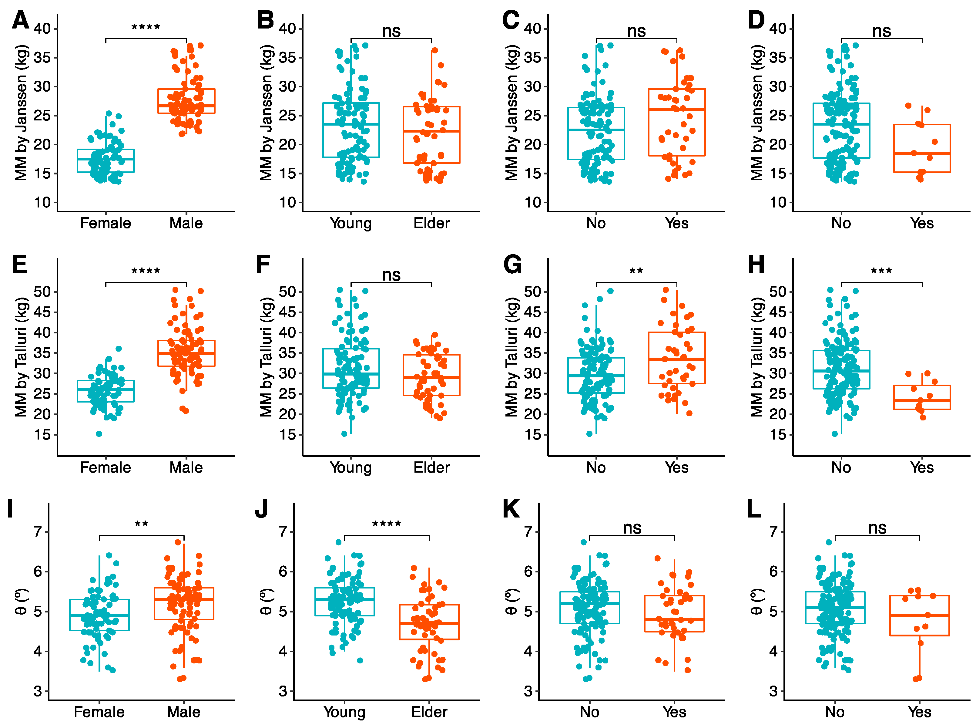
| Janssen MM (kg) [34] | Talluri MM (kg) | Kanellakis FFM (kg) [36] | Kotler FFM (kg) [37] | Talluri FFM (kg) | θ (°) | |
| Whole sample | : 22.9 (6.1) M: 23.3 (9.2) [13.6, 37.1] | : 30.8 (7.0) M: 29.9 (9.4) [15.2, 50.5] | : 31.3 (12.0) M: 32.6 (19.1) [6.4, 58.2] | : 48.1 (9.2) M: 47.7 (13.1) [30.6, 74.5] | : 50.7 (9.7) M: 49.9 (14.2) [33.4, 80.1] | : 5.0 (0.7) M: 5.1 (0.9) [2.6, 6.7] |
| Sex Male Female p | 26.7 17.5 <2.2 × 10⁻¹⁶ | 34.9 26.0 <2.2 × 10⁻¹⁶ | 40.3 21.1 <2.2 × 10⁻¹⁶ | 52.8 40.7 <2.2 × 10⁻¹⁶ | 56.8 42.6 <2.2 × 10⁻¹⁶ | 5.3 4.9 0.002 |
| Age Young Elder p | 23.5 22.3 0.287 | 29.9 29.0 0.103 | 33.5 32.0 0.865 | 47.7 47.9 0.719 | 50.4 49.1 0.807 | 5.3 4.7 2.44 × 10⁻⁶ |
| Obesity No obesity Obesity p | 22.5 26.1 0.041 | 29.4 33.5 8.258 × 10⁻³ | 30.5 38.2 1.596 × 10⁻³ | 45.7 53.0 7.969 × 10⁻⁴ | 48.5 55.2 5.229 × 10⁻⁴ | 5.2 4.8 0.277 |
| GLIM Negative Positive p | 23.5 18.5 0.050 | 30.6 23.5 5.171 × 10⁻⁴ | 33.5 18.8 0.003 | 48.7 41.5 0.006 | 50.5 41.4 9.361 × 10⁻⁴ | 5.1 4.90.327 |
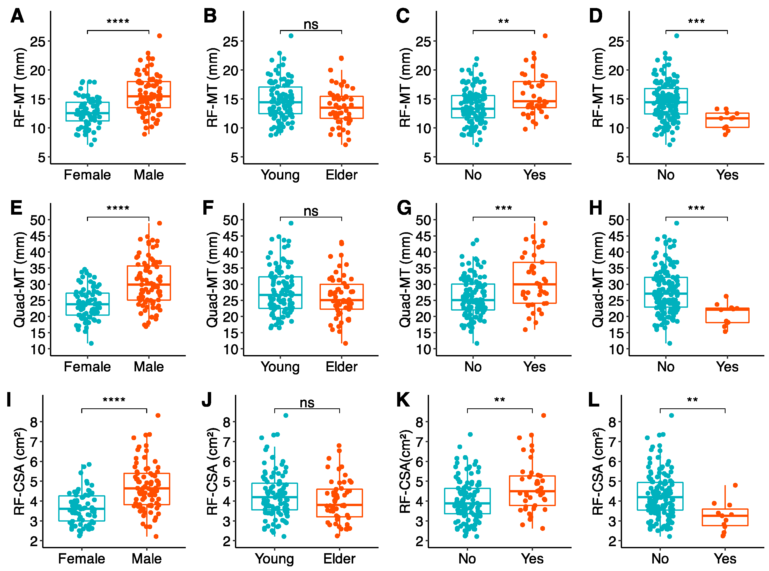
| RF-MT (mm) | Quad-MT (mm) | RF-CSA (cm2) | HGS (kg) | |
|---|---|---|---|---|
| Whole sample | : 14.3(3.3) M: 13.9(3.9) [7.1, 25.9] | : 27.3(7.0) M: 26.6(9.1) [11.7, 48.9] | : 4.2(1.2) M: 4.1(1.4) [1.7, 8.3] | : 34.8 (10.0) M: 33.9 (12.9) [13.3, 64.0] |
| Sex Male Female p | 15.4 12.5 5.154 × 10⁻⁹ | 29.9 23.8 6.309 × 10⁻⁹ | 4.64 3.60 8.208 × 10⁻⁹ | 40.0 29.0 1.7 × 10⁻¹³ |
| Age Young Elder p | 14.4 13.5 0.082 | 26.7 25.1 0.214 | 4.19 3.79 0.121 | 36.4 31.6 0.006 |
| Obesity No obesity Obesity p | 13.3 14.6 3.164 × 10⁻³ | 25.1 30.0 8.568 × 10⁻³ | 3.9 4.5 1.794 × 10⁻³ | 34.6 35.5 0.655 |
| GLIM Negative Positive p | 14.4 11.7 7.204 × 10⁻³ | 27.1 22.1 2.502 × 10⁻⁴ | 4.18 3.26 0.002 | 35.0 32.1 0.407 |
Disclaimer/Publisher’s Note: The statements, opinions and data contained in all publications are solely those of the individual author(s) and contributor(s) and not of MDPI and/or the editor(s). MDPI and/or the editor(s) disclaim responsibility for any injury to people or property resulting from any ideas, methods, instructions or products referred to in the content. |
© 2024 by the authors. Licensee MDPI, Basel, Switzerland. This article is an open access article distributed under the terms and conditions of the Creative Commons Attribution (CC BY) license (https://creativecommons.org/licenses/by/4.0/).
Share and Cite
Jiménez-Sánchez, A.; Soriano-Redondo, M.E.; Roque-Cuéllar, M.d.C.; García-Rey, S.; Valladares-Ayerbes, M.; Pereira-Cunill, J.L.; García-Luna, P.P. Muscle Biomarkers in Colorectal Cancer Outpatients: Agreement Between Computed Tomography, Bioelectrical Impedance Analysis, and Nutritional Ultrasound. Nutrients 2024, 16, 4312. https://doi.org/10.3390/nu16244312
Jiménez-Sánchez A, Soriano-Redondo ME, Roque-Cuéllar MdC, García-Rey S, Valladares-Ayerbes M, Pereira-Cunill JL, García-Luna PP. Muscle Biomarkers in Colorectal Cancer Outpatients: Agreement Between Computed Tomography, Bioelectrical Impedance Analysis, and Nutritional Ultrasound. Nutrients. 2024; 16(24):4312. https://doi.org/10.3390/nu16244312
Chicago/Turabian StyleJiménez-Sánchez, Andrés, María Elisa Soriano-Redondo, María del Carmen Roque-Cuéllar, Silvia García-Rey, Manuel Valladares-Ayerbes, José Luis Pereira-Cunill, and Pedro Pablo García-Luna. 2024. "Muscle Biomarkers in Colorectal Cancer Outpatients: Agreement Between Computed Tomography, Bioelectrical Impedance Analysis, and Nutritional Ultrasound" Nutrients 16, no. 24: 4312. https://doi.org/10.3390/nu16244312
APA StyleJiménez-Sánchez, A., Soriano-Redondo, M. E., Roque-Cuéllar, M. d. C., García-Rey, S., Valladares-Ayerbes, M., Pereira-Cunill, J. L., & García-Luna, P. P. (2024). Muscle Biomarkers in Colorectal Cancer Outpatients: Agreement Between Computed Tomography, Bioelectrical Impedance Analysis, and Nutritional Ultrasound. Nutrients, 16(24), 4312. https://doi.org/10.3390/nu16244312