
Automated Detection of Caffeinated Coffee-Induced Short-Term Effects on ECG Signals Using EMD, DWT, and WPD


Abstract
:1. Introduction
2. Materials and Methods
2.1. Dataset
2.2. Pre-Processing and Noise Elimination
2.3. ECG Decomposition Methods
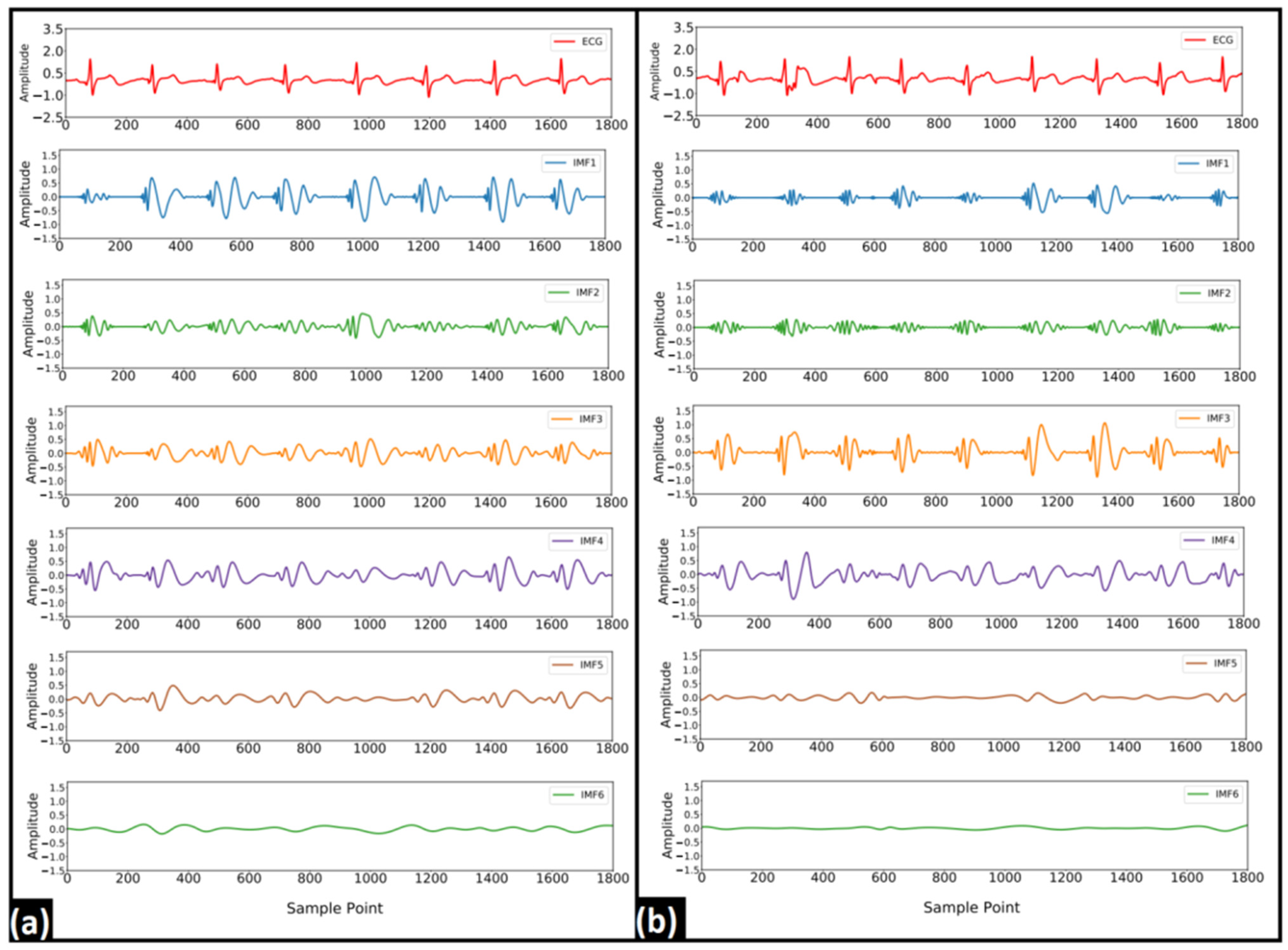
2.3.1. Empirical Mode Decomposition
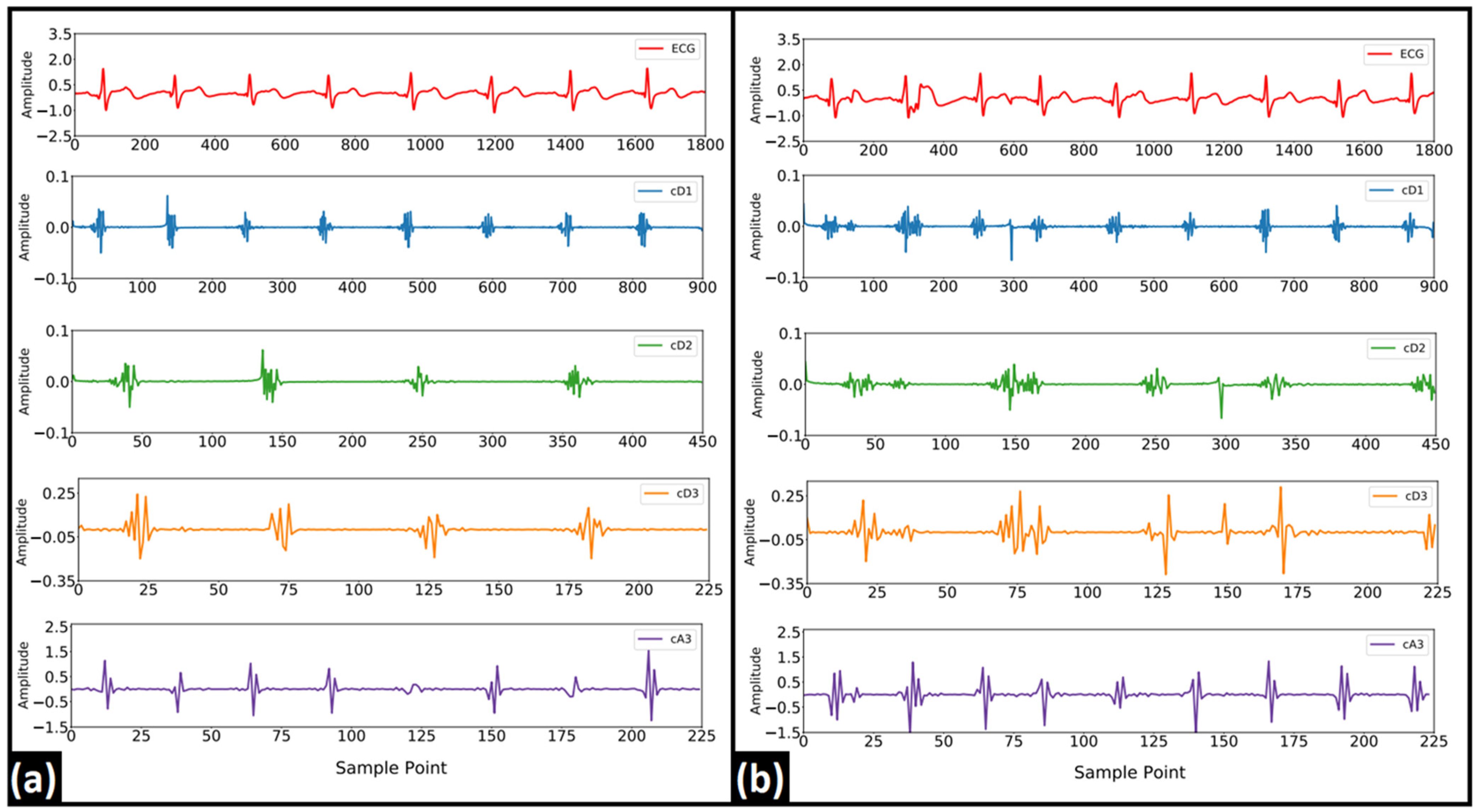
2.3.2. Discrete Wavelet Transform
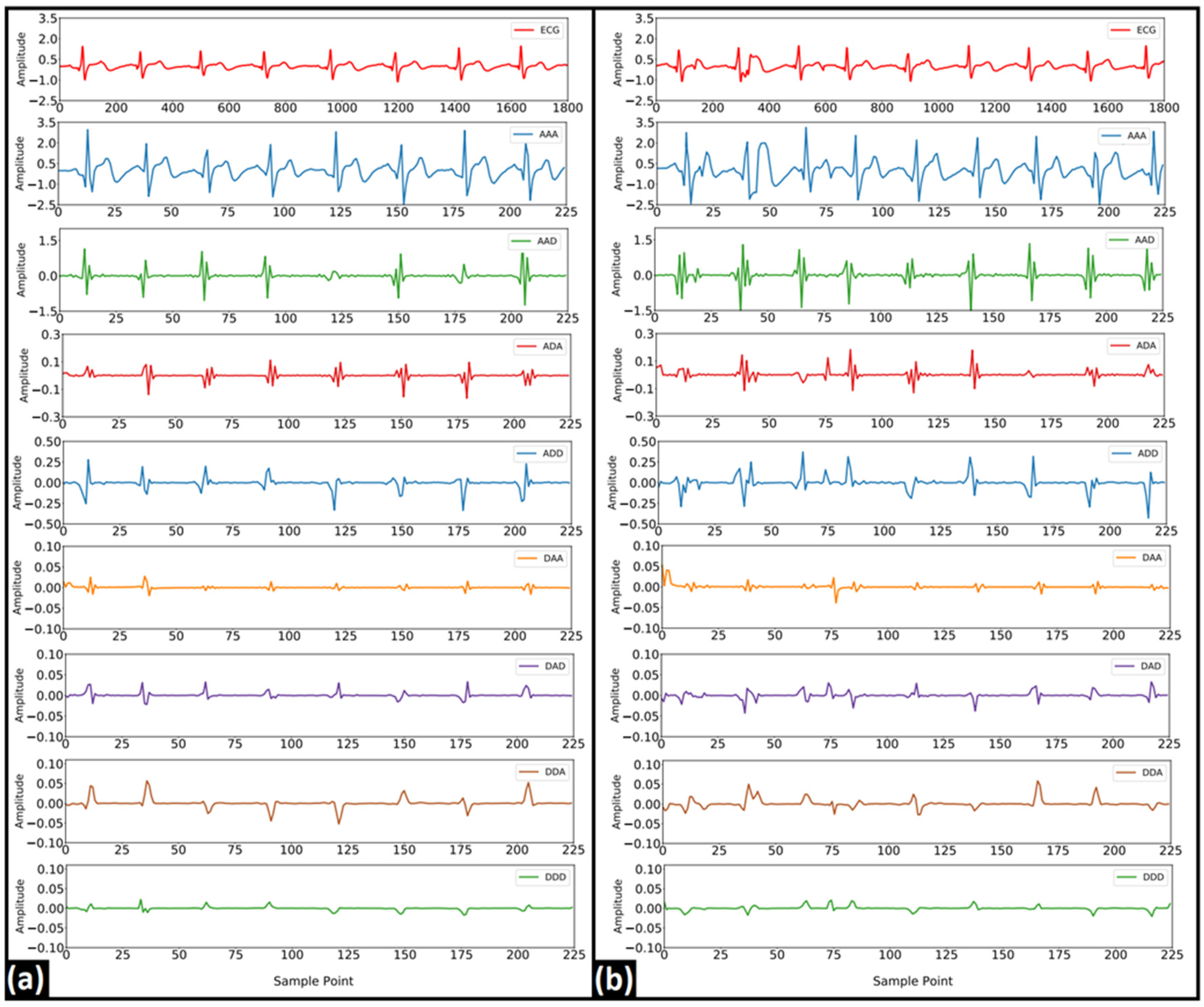
2.3.3. Wavelet Packet Decomposition
2.4. Feature Extraction and Selection
2.5. Classification Using Machine Learning Models
2.6. Validation and Evaluation of the ML Models
3. Results
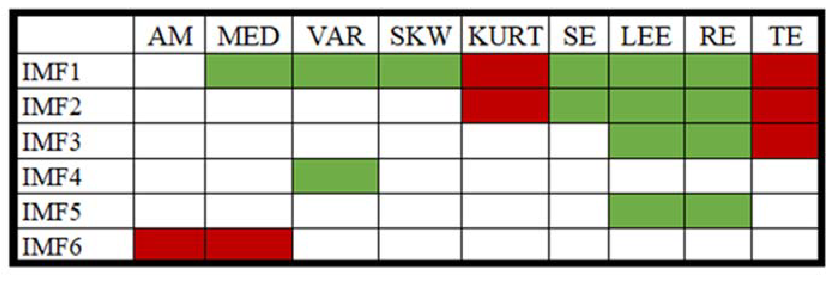
3.1. EMD Analysis
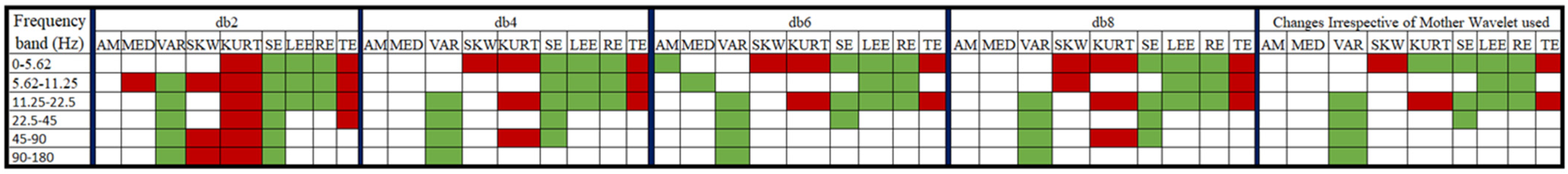
3.2. DWT Analysis
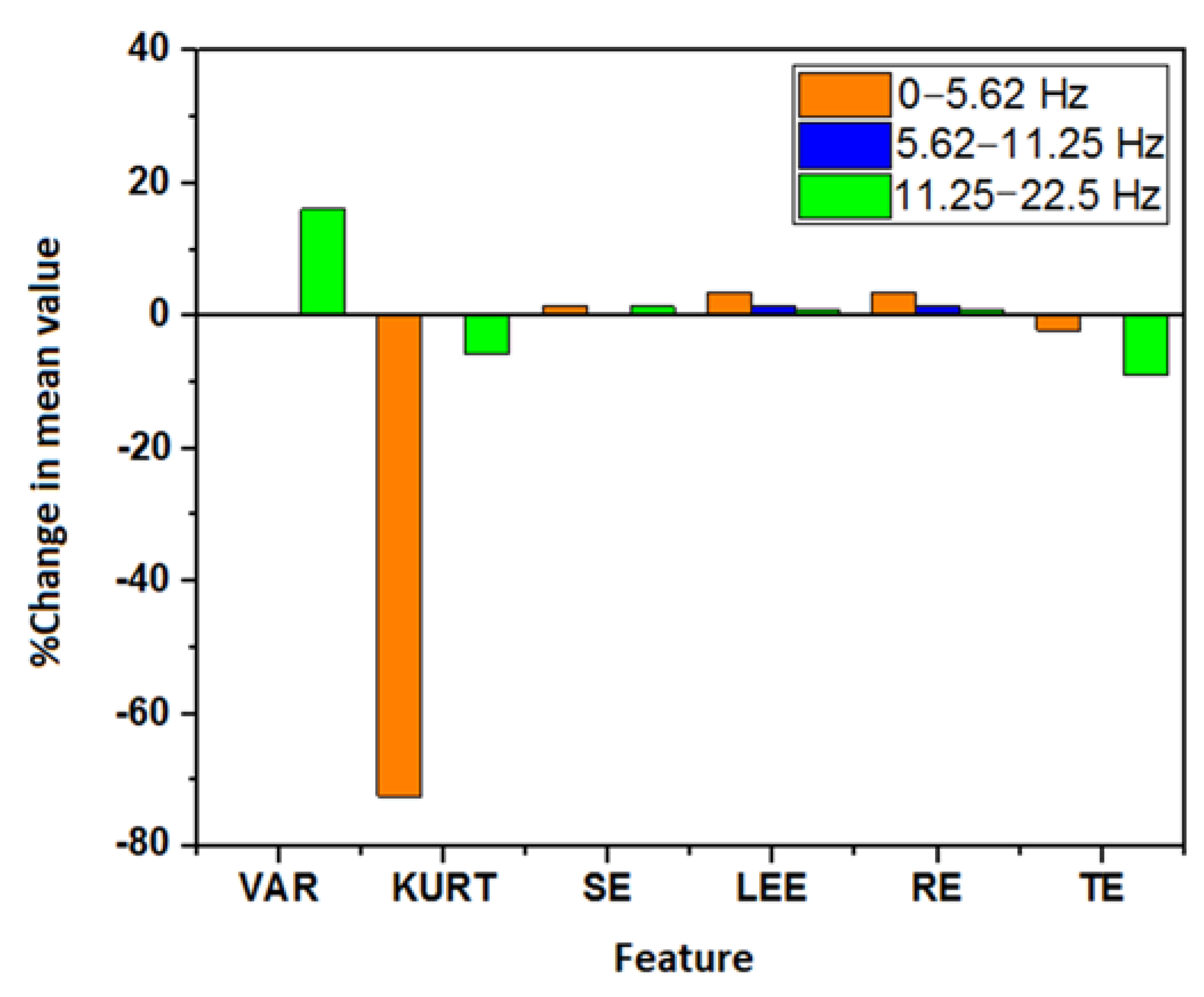
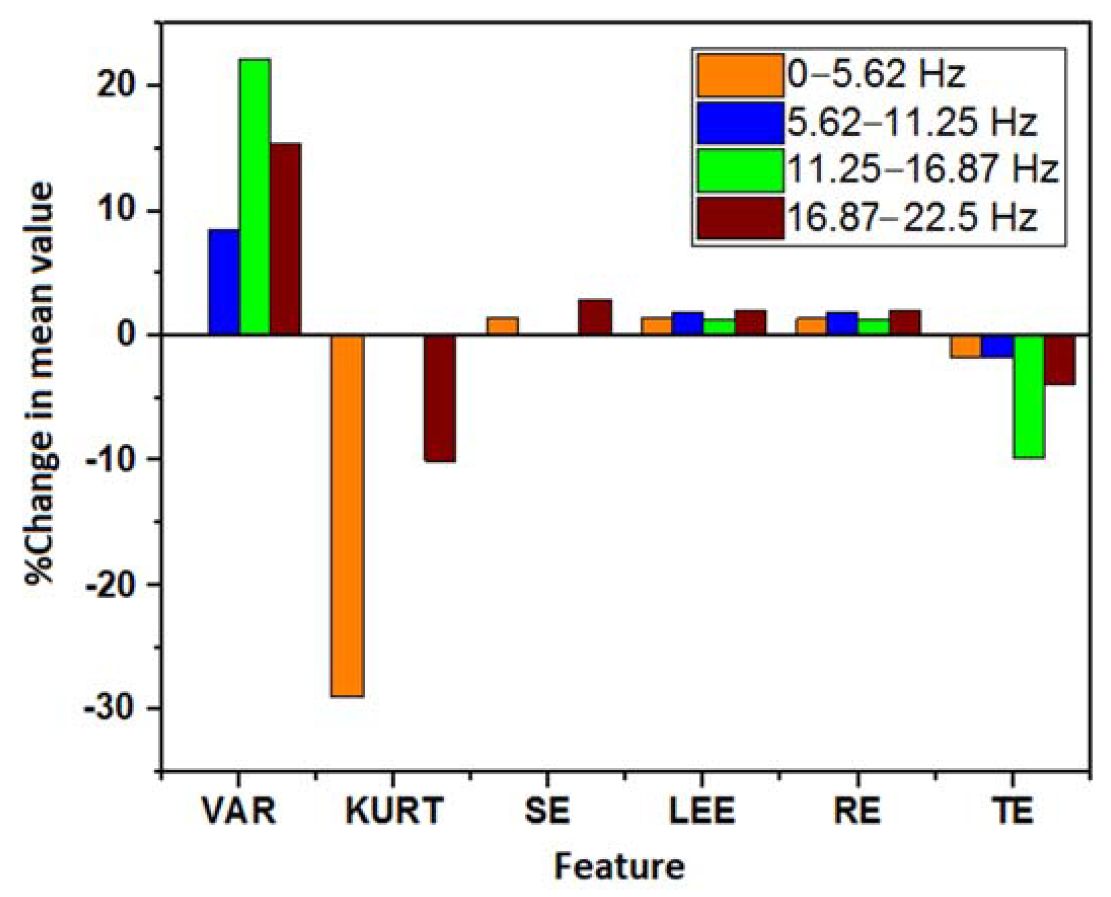
3.3. WPD Analysis
4. Discussions
5. Limitations, Future Work, and Conclusions
Supplementary Materials
Author Contributions
Funding
Institutional Review Board Statement
Informed Consent Statement
Data Availability Statement
Conflicts of Interest
References
- Rauh, R.; Burkert, M.; Siepmann, M.; Mueck-Weymann, M. Acute effects of caffeine on heart rate variability in habitual caffeine consumers. Clin. Physiol. Funct. Imaging 2006, 26, 163–166. [Google Scholar] [CrossRef]
- Gramza-Michałowska, A. Caffeine in tea Camellia sinensis—Content, absorption, benefits and risks of consumption. J. Nutr. Health Aging 2014, 18, 143–149. [Google Scholar] [CrossRef] [PubMed]
- Harland, B.F. Caffeine and nutrition. Nutrition 2000, 16, 522–526. [Google Scholar] [CrossRef]
- Graham, T.E. Caffeine and exercise. Sports Med. 2001, 31, 785–807. [Google Scholar] [CrossRef] [PubMed]
- Gramza-Michałowska, A.; Sidor, A.; Kulczyński, B. Methylxanthines in Food Products. In Analytical Methods in the Determination of Bioactive Compounds and Elements in Food: Food Bioactive Ingredients; Jeszka-Skowron, M., Zgoła-Grześkowiak, A., Grześkowiak, T., Ramakrishna, A., Eds.; Springer Nature: Cham, Switzerland, 2021; pp. 83–100. [Google Scholar]
- Goldstein, E.R.; Ziegenfuss, T.; Kalman, D.; Kreider, R.; Campbell, B.; Wilborn, C.; Taylor, L.; Willoughby, D.; Stout, J.; Graves, B.S. International society of sports nutrition position stand: Caffeine and performance. J. Int. Soc. Sports Nutr. 2010, 7, 5. [Google Scholar] [CrossRef] [PubMed] [Green Version]
- Adan, A.; Prat, G.; Fabbri, M.; Sànchez-Turet, M. Early effects of caffeinated and decaffeinated coffee on subjective state and gender differences. Prog. Neuro-Psychopharmacol. Biol. Psychiatry 2008, 32, 1698–1703. [Google Scholar] [CrossRef] [PubMed]
- Grant, S.S.; Magruder, K.P.; Friedman, B.H. Controlling for caffeine in cardiovascular research: A critical review. Int. J. Psychophysiol. 2018, 133, 193–201. [Google Scholar] [CrossRef] [PubMed]
- Benowitz, N.L. Clinical pharmacology of caffeine. Annu. Rev. Med. 1990, 41, 277–288. [Google Scholar] [CrossRef]
- Koenig, J.; Jarczok, M.N.; Kuhn, W.; Morsch, K.; Schäfer, A.; Hillecke, T.K.; Thayer, J.F. Impact of Caffeine on Heart Rate Variability: A Systematic Review. J. Caffeine Res. 2013, 3, 22–37. [Google Scholar] [CrossRef]
- Dömötör, Z.; Szemerszky, R.; Köteles, F. Subjective and objective effects of coffee consumption—Caffeine or expectations? Acta Physiol. Hung. 2015, 102, 77–85. [Google Scholar] [CrossRef]
- De Oliveira, R.A.M.; Araújo, L.F.; de Figueiredo, R.C.; Goulart, A.C.; Schmidt, M.I.; Barreto, S.M.; Ribeiro, A.L.P. Coffee Consumption and Heart Rate Variability: The Brazilian Longitudinal Study of Adult Health (ELSA-Brasil) Cohort Study. Nutrients 2017, 9, 741. [Google Scholar] [CrossRef] [PubMed] [Green Version]
- Sarshin, A.; Naderi, A.; da Cruz, C.J.G.; Feizolahi, F.; Forbes, S.C.; Candow, D.G.; Mohammadgholian, E.; Amiri, M.; Jafari, N.; Rahimi, A.; et al. The effects of varying doses of caffeine on cardiac parasympathetic reactivation following an acute bout of anaerobic exercise in recreational athletes. J. Int. Soc. Sports Nutr. 2020, 17, 44. [Google Scholar] [CrossRef] [PubMed]
- Karayigit, R.; Naderi, A.; Akca, F.; Cruz, C.J.G.D.; Sarshin, A.; Yasli, B.C.; Ersoz, G.; Kaviani, M. Effects of Different Doses of Caffeinated Coffee on Muscular Endurance, Cognitive Performance, and Cardiac Autonomic Modulation in Caffeine Naive Female Athletes. Nutrients 2020, 13, 2. [Google Scholar] [CrossRef] [PubMed]
- Caldeira, D.; Martins, C.; Alves, L.B.; Pereira, H.; Ferreira, J.J.; Costa, J. Caffeine does not increase the risk of atrial fibrillation: A systematic review and meta-analysis of observational studies. Heart 2013, 99, 1383–1389. [Google Scholar] [CrossRef] [PubMed]
- Gaeini, Z.; Bahadoran, Z.; Mirmiran, P.; Azizi, F. Tea, coffee, caffeine intake and the risk of cardiometabolic outcomes: Findings from a population with low coffee and high tea consumption. Nutr. Metab. 2019, 16, 28. [Google Scholar] [CrossRef] [PubMed]
- Shah, S.A.; Szeto, A.H.; Farewell, R.; Shek, A.; Fan, D.; Quach, K.N.; Bhattacharyya, M.; Elmiari, J.; Chan, W.; O’Dell, K.; et al. Impact of High Volume Energy Drink Consumption on Electrocardiographic and Blood Pressure Parameters: A Randomized Trial. J. Am. Heart Assoc. 2019, 8, e011318. [Google Scholar] [CrossRef] [PubMed] [Green Version]
- Zimmermann-Viehoff, F.; Thayer, J.; Koenig, J.; Herrmann, C.; Weber, C.S.; Deter, H.C. Short-term effects of espresso coffee on heart rate variability and blood pressure in habitual and non-habitual coffee consumers-a randomized crossover study. Nutr. Neurosci. 2016, 19, 169–175. [Google Scholar] [CrossRef] [PubMed]
- Prineas, R.J.; Jacobs, D.R., Jr.; Crow, R.S.; Blackburn, H. Coffee, tea and VPB. J. Chronic Dis. 1980, 33, 67–72. [Google Scholar] [CrossRef]
- Sutherland, D.J.; McPherson, D.D.; Renton, K.W.; Spencer, C.A.; Montague, T.J. The effect of caffeine on cardiac rate, rhythm, and ventricular repolarization. Analysis of 18 normal subjects and 18 patients with primary ventricular dysrhythmia. Chest 1985, 87, 319–324. [Google Scholar] [CrossRef]
- Myers, M.G.; Harris, L.; Leenen, F.H.; Grant, D.M. Caffeine as a possible cause of ventricular arrhythmias during the healing phase of acute myocardial infarction. Am. J. Cardiol. 1987, 59, 1024–1028. [Google Scholar] [CrossRef]
- Brothers, R.M.; Christmas, K.M.; Patik, J.C.; Bhella, P.S. Heart rate, blood pressure and repolarization effects of an energy drink as compared to coffee. Clin. Physiol. Funct. Imaging 2017, 37, 675–681. [Google Scholar] [CrossRef] [PubMed]
- Smits, P.; Thien, T.; Van’t Laar, A. The cardiovascular effects of regular and decaffeinated coffee. Br. J. Clin. Pharmacol. 1985, 19, 852–854. [Google Scholar] [CrossRef] [PubMed] [Green Version]
- Hajsadeghi, S.; Mohammadpour, F.; Manteghi, M.J.; Kordshakeri, K.; Tokazebani, M.; Rahmani, E.; Hassanzadeh, M. Effects of energy drinks on blood pressure, heart rate, and electrocardiographic parameters: An experimental study on healthy young adults. Anatol. J. Cardiol. 2016, 16, 94–99. [Google Scholar] [CrossRef] [PubMed]
- Nurmaini, S.; Darmawahyuni, A.; Sakti Mukti, A.N.; Rachmatullah, M.N.; Firdaus, F.; Tutuko, B. Deep Learning-Based Stacked Denoising and Autoencoder for ECG Heartbeat Classification. Electronics 2020, 9, 135. [Google Scholar] [CrossRef] [Green Version]
- Chiang, H.-T.; Hsieh, Y.-Y.; Fu, S.-W.; Hung, K.-H.; Tsao, Y.; Chien, S.-Y. Noise Reduction in ECG Signals Using Fully Convol Noise reduction in ECG signals using fully convolutional denoising autoencoders. IEEE Access 2019, 7, 60806–60813. [Google Scholar] [CrossRef]
- Jenkal, W.; Latif, R.; Toumanari, A.; Dliou, A.; El B’charri, O.; Maoulainine, F.M. An efficient algorithm of ECG signal denoising using the adaptive dual threshold filter and the discrete wavelet transform. Biocybern. Biomed. Eng. 2016, 36, 499–508. [Google Scholar] [CrossRef]
- Pradhan, B.K.; Pal, K. Statistical and entropy-based features can efficiently detect the short-term effect of caffeinated coffee on the cardiac physiology. Med. Hypotheses 2020, 145, 110323. [Google Scholar] [CrossRef] [PubMed]
- Song, L.; Yu, F. The time-frequency analysis of abnormal ECG signals. In Life System Modeling and Intelligent Computing; Li, K., Jia, L., Sun, X., Fei, M., Irwin, G.W., Eds.; Springer: Berlin/Heidelberg, Germany, 2010; pp. 60–66. [Google Scholar]
- Chatterjee, S.; Thakur, R.S.; Yadav, R.N.; Gupta, L.; Raghuvanshi, D.K. Review of noise removal techniques in ECG signals. IET Signal Process. 2020, 14, 569–590. [Google Scholar] [CrossRef]
- Castillo, E.; Morales, D.P.; García, A.; Martínez-Martí, F.; Parrilla, L.; Palma, A.J. Noise suppression in ECG signals through efficient one-step wavelet processing techniques. J. Appl. Math. 2013, 2013, 763903. [Google Scholar] [CrossRef]
- Zhu, W.; Zhao, W.; Chen, X. A new QRS detector based on empirical mode decomposition. In Proceedings of the IEEE 10th International Conference on Signal Processing Proceedings ICSP, Beijing, China, 24–28 October 2010; pp. 1–4. [Google Scholar]
- Kumar, S.; Panigrahy, D.; Sahu, P. Denoising of Electrocardiogram (ECG) signal by using empirical mode decomposition (EMD) with non-local mean (NLM) technique. Biocybern. Biomed. Eng. 2018, 38, 297–312. [Google Scholar] [CrossRef]
- Khorrami, H.; Moavenian, M. A comparative study of DWT, CWT and DCT transformations in ECG arrhythmias classification. Expert Syst. Appl. 2010, 37, 5751–5757. [Google Scholar] [CrossRef]
- Zhang, J.; Liu, A.; Gao, M.; Chen, X.; Zhang, X.; Chen, X. ECG-based multi-class arrhythmia detection using spatio-temporal attention-based convolutional recurrent neural network. Artif. Intell. Med. 2020, 106, 101856. [Google Scholar] [CrossRef] [PubMed]
- Ranaee, V.; Ebrahimzadeh, A.; Ghaderi, R. Application of the PSO–SVM model for recognition of control chart patterns. ISA Trans. 2010, 49, 577–586. [Google Scholar] [CrossRef]
- Ramsey, F.; Schafer, D. The Statistical Sleuth: A Course in Methods of Data Analysis; Cengage Learning: Boston, MA, USA, 2012. [Google Scholar]
- Li, T.; Zhou, M. ECG classification using wavelet packet entropy and random forests. Entropy 2016, 18, 285. [Google Scholar] [CrossRef]
- Das, K.R.; Imon, A. A brief review of tests for normality. Am. J. Theor. Appl. Stat. 2016, 5, 5–12. [Google Scholar]
- Pławiak, P.; Acharya, U.R. Novel deep genetic ensemble of classifiers for arrhythmia detection using ECG signals. Neural Comput. Appl. 2020, 32, 11137–11161. [Google Scholar] [CrossRef] [Green Version]
- Nayak, S.K.; Pradhan, B.K.; Banerjee, I.; Pal, K. Analysis of heart rate variability to understand the effect of cannabis consumption on Indian male paddy-field workers. Biomed. Signal Process. Control 2020, 62, 102072. [Google Scholar] [CrossRef]
- Padmavathi, S.; Ramanujam, E. Naïve Bayes classifier for ECG abnormalities using multivariate maximal time series motif. Procedia Comput. Sci. 2015, 47, 222–228. [Google Scholar] [CrossRef] [Green Version]
- Raghu, S.; Sriraam, N.; Temel, Y.; Rao, S.V.; Hegde, A.S.; Kubben, P.L. Performance evaluation of DWT based sigmoid entropy in time and frequency domains for automated detection of epileptic seizures using SVM classifier. Comput. Biol. Med. 2019, 110, 127–143. [Google Scholar] [CrossRef]
- Akhbardeh, A.; Farrokhi, M.; Tehrani, A.V. EEG features extraction using neuro-fuzzy systems and shift-invariant wavelet transforms for epileptic seizures diagnosing. In Proceedings of the 26th Annual International Conference of the IEEE Engineering in Medicine and Biology Society, San Francisco, CA, USA, 1–5 September 2004; pp. 498–502. [Google Scholar]
- Acharya, U.R.; Fujita, H.; Lih, O.S.; Adam, M.; Tan, J.H.; Chua, C.K. Automated detection of coronary artery disease using different durations of ECG segments with convolutional neural network. Knowl.-Based Syst. 2017, 132, 62–71. [Google Scholar] [CrossRef]
- Acharya, U.R.; Fujita, H.; Lih, O.S.; Hagiwara, Y.; Tan, J.H.; Adam, M. Automated detection of arrhythmias using different intervals of tachycardia ECG segments with convolutional neural network. Inf. Sci. 2017, 405, 81–90. [Google Scholar] [CrossRef]
- Sinha, N.; Das, A. Discrimination of Life-Threatening Arrhythmias Using Singular Value, Harmonic Phase Distribution, and Dynamic Time Warping of ECG Signals. IEEE Trans. Instrum. Meas. 2020, 70, 1–8. [Google Scholar] [CrossRef]
- Sellami, A.; Zouaghi, A.; Daamouche, A. ECG as a biometric for individual’s identification. In Proceedings of the 2017 5th International Conference on Electrical Engineering-Boumerdes (ICEE-B), Boumerdes, Algeria, 29–31 October 2017; pp. 1–6. [Google Scholar]
- Mahmoodabadi, S.; Ahmadian, A.; Abolhasani, M. ECG feature extraction using Daubechies wavelets. In Proceedings of the 5th IASTED International Conference on Visualization, Imaging and Image Processing, Benidorm, Spain, 7–9 September 2005; pp. 343–348. [Google Scholar]
- Sasikala, P.; Wahidabanu, R. Robust r peak and qrs detection in electrocardiogram using wavelet transform. Int. J. Adv. Comput. Sci. Appl.-IJACSA 2010, 1, 48–53. [Google Scholar] [CrossRef]
- Uddin, M.B.; Hossain, M.; Ahmad, M.; Ahmed, N.; Rashid, M.A. Effects of caffeinated beverage consumption on electrocardiographic parameters among healthy adults. Mod. Appl. Sci. 2014, 8, 69. [Google Scholar] [CrossRef] [Green Version]
- Kumar, P.; Verma, D.K.; Narayan, J.; Kanawjia, P.; Ghildiyal, A. Effect of coffee on blood pressure and electrocardiographic changes in nicotine users. Asian J. Med. Sci. 2015, 6, 46–48. [Google Scholar] [CrossRef] [Green Version]
- Molnar, J.; Somberg, J.C. A rapid method to evaluate cardiac repolarization Changes: The effect of two coffee strengths on the QT interval. Cardiology 2015, 131, 203–208. [Google Scholar] [CrossRef]
- Kozik, T.M.; Shah, S.; Bhattacharyya, M.; Franklin, T.T.; Connolly, T.F.; Chien, W.; Charos, G.S.; Pelter, M.M. Cardiovascular responses to energy drinks in a healthy population: The C-energy study. Am. J. Emerg. Med. 2016, 34, 1205–1209. [Google Scholar] [CrossRef]
- Tauseef, A.; Akmal, A.; Hasan, S.; Waheed, A.; Zafar, A.; Cheema, A.; Mukhtar, Q.; Malik, A. Effect of energy drink on reaction time, haemodynamic and electrocardiographic parameters. Pak. J. Physiol. 2017, 13, 7–10. [Google Scholar]
- Aziz, S.; Khan, M.U.; Choudhry, A.; Aymin, A.; Usman, A. ECG-based Biometric Authentication using Empirical Mode Decomposition and Support Vector Machines. In Proceedings of the 2019 IEEE 10th Annual Information Technology, Electronics and Mobile Communication Conference (IEMCON), Vancouver, BC, Canada, 17–19 October 2019; pp. 0906–0912. [Google Scholar]
- Kumar, M.; Pachori, R.B.; Acharya, U.R. Automated diagnosis of atrial fibrillation ECG signals using entropy features extracted from flexible analytic wavelet transform. Biocybern. Biomed. Eng. 2018, 38, 564–573. [Google Scholar] [CrossRef]
- Caliskan, S.G.; Bilgin, M.D. Non-linear analysis of heart rate variability for evaluating the acute effects of caffeinated beverages in young adults. Cardiol. Young 2020, 30, 1018–1023. [Google Scholar] [CrossRef]
- Turley, K.R.; Rivas, J.D.; Townsend, J.R.; Morton, A.B. Effects of caffeine on heart rate variability in boys. J. Caffeine Res. 2017, 7, 71–77. [Google Scholar] [CrossRef]
- Shah, S.A.; Dargush, A.E.; Potts, V.; Lee, M.; Millard-Hasting, B.M.; Williams, B.; Lacey, C.S. Effects of single and multiple energy shots on blood pressure and electrocardiographic parameters. Am. J. Cardiol. 2016, 117, 465–468. [Google Scholar] [CrossRef] [PubMed]
- Li, J.; Deng, G.; Wei, W.; Wang, H.; Ming, Z. Design of a real-time ECG filter for portable mobile medical systems. IEEE Access 2016, 5, 696–704. [Google Scholar] [CrossRef]
- Rajesh, K.N.; Dhuli, R. Classification of ECG heartbeats using non-linear decomposition methods and support vector machine. Comput. Biol. Med. 2017, 87, 271–284. [Google Scholar] [CrossRef] [PubMed]
- Nygaard, H.; Riksaasen, S.; Hjelmevoll, L.M.; Wold, E. Effect of caffeine ingestion on competitive rifle shooting performance. PLoS ONE 2019, 14, e0224596. [Google Scholar] [CrossRef] [PubMed]
- Dall’Acqua, F.; Cristina-Souza, G.; Santos-Mariano, A.; Bertuzzi, R.; Rodacki, C.; Lima-Silva, A. Caffeine ingestion improves specific artistic swimming tasks. Braz. J. Med. Biol. Res. 2021, 54, e10346. [Google Scholar] [CrossRef]
- Rocha, J.C.C.; da Rocha, A.L.S.; da Silva Santos Soares, G.; Correia-Oliveira, C.R. Effects of caffeine ingestion on upper and lower limb muscle power of handball players: A double-blind, placebo-controlled, crossover study. Sport Sci. Health 2021, 17, 1039–1044. [Google Scholar] [CrossRef]
- Burke, B.I.; Travis, S.K.; Gentles, J.A.; Sato, K.; Lang, H.M.; Bazyler, C.D. The effects of caffeine on jumping performance and maximal strength in female collegiate athletes. Nutrients 2021, 13, 2496. [Google Scholar] [CrossRef]
- Aguilar-Navarro, M.; Muñoz, G.; Salinero, J.J.; Muñoz-Guerra, J.; Fernández-Álvarez, M.; Plata, M.d.M.; Del Coso, J. Urine caffeine concentration in doping control samples from 2004 to 2015. Nutrients 2019, 11, 286. [Google Scholar] [CrossRef] [Green Version]
- Maji, U.; Mitra, M.; Pal, S. Characterization of cardiac arrhythmias by variational mode decomposition technique. Biocybern. Biomed. Eng. 2017, 37, 578–589. [Google Scholar] [CrossRef]


 : a significant decrease in value post-consumption of coffee,
  : a significant increase in value post-consumption of coffee, no color: insignificant change in value post-consumption of coffee).
: a significant decrease in value post-consumption of coffee, : a significant increase in value post-consumption of coffee, no color: insignificant change in value post-consumption of coffee).
: a significant increase in value post-consumption of coffee, no color: insignificant change in value post-consumption of coffee).
: a significant decrease in value post-consumption of coffee, : a significant increase in value post-consumption of coffee, no color: insignificant change in value post-consumption of coffee).
 : a significant decrease in value post-consumption of coffee, : a significant increase in value post-consumption of coffee, no color: insignificant change in value).
: a significant decrease in value post-consumption of coffee, : a significant increase in value post-consumption of coffee, no color: insignificant change in value).
: a significant decrease in value post-consumption of coffee, : a significant increase in value post-consumption of coffee, no color: insignificant change in value).

 : a significant decrease in value post-consumption of coffee, : a significant increase in value post-consumption of coffee, no color: insignificant change in value post-consumption of coffee).
: a significant decrease in value post-consumption of coffee, : a significant increase in value post-consumption of coffee, no color: insignificant change in value post-consumption of coffee).
: a significant decrease in value post-consumption of coffee, : a significant increase in value post-consumption of coffee, no color: insignificant change in value post-consumption of coffee).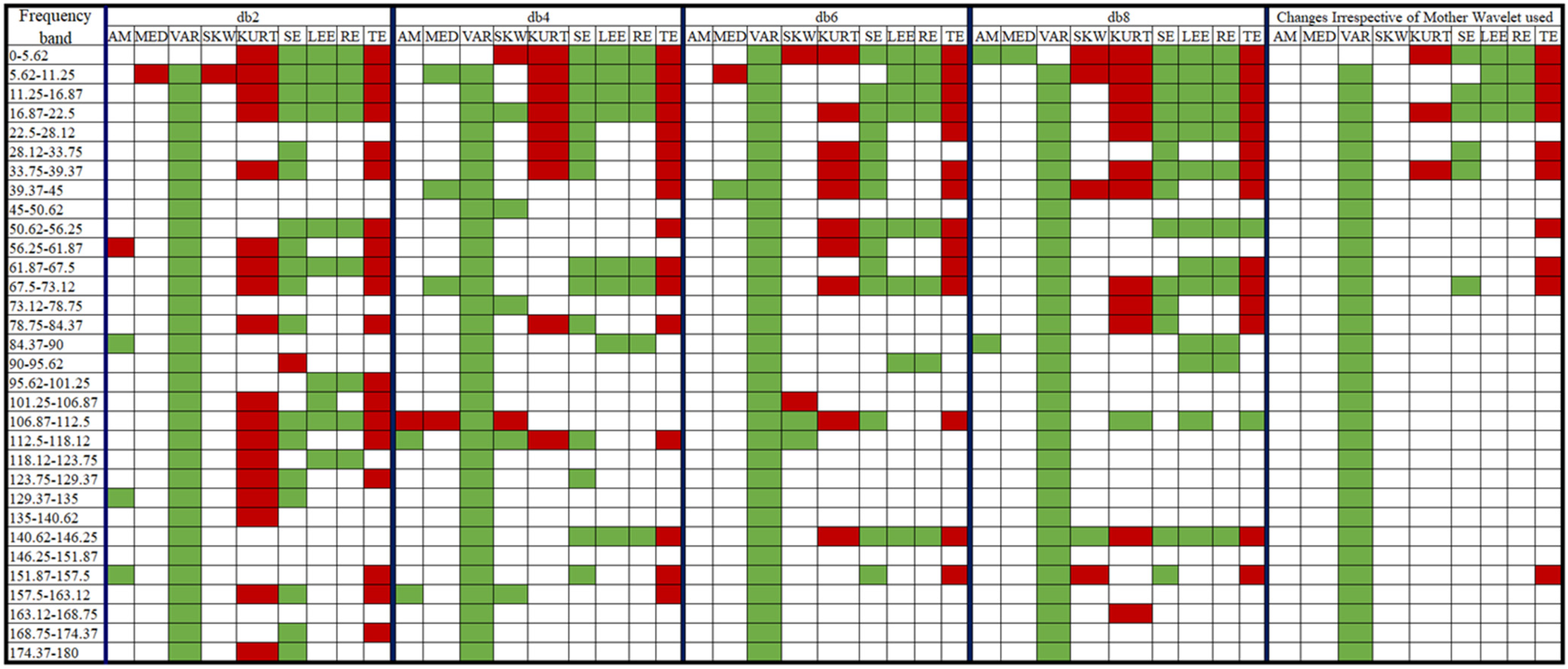


| No. of IMFs | ML Model | Accuracy | Precision | F-Measure | Sensitivity | Specificity | AUC |
|---|---|---|---|---|---|---|---|
| 1 | DL | 56.11 ± 2.11 | 54.08 ± 1.59 | 65.21 ± 0.89 | 82.22 ± 2.48 | 30.00 ± 6.02 | 0.615 ± 0.055 |
| 2 | GBT | 53.61 ± 2.52 | 52.77 ± 1.91 | 59.25 ± 3.64 | 67.78 ± 7.24 | 39.44 ± 5.34 | 0.579 ± 0.019 |
| 3 | FLM | 53.89 ± 2.67 | 53.10 ± 2.26 | 59.69 ± 2.02 | 68.33 ± 4.21 | 39.44 ± 6.63 | 0.551 ± 0.041 |
| 4 | DL | 57.50 ± 2.32 | 57.12 ± 2.08 | 58.48 ± 3.01 | 60.00 ± 4.65 | 55.00 ± 3.04 | 0.587 ± 0.047 |
| 5 | DL | 53.06 ± 2.06 | 52.10 ± 1.39 | 61.84 ± 1.75 | 76.11 ± 3.17 | 30.00 ± 3.62 | 0.565 ± 0.050 |
| 6 | GBT | 53.61 ± 1.24 | 52.73 ± 1.04 | 60.66 ± 1.17 | 71.67 ± 5.34 | 35.56 ± 7.71 | 0.554 ± 0.024 |
 maximum value.
| Level | Wavelet Used | ML Model | Accuracy | Precision | F-Measure | Sensitivity | Specificity | AUC |
|---|---|---|---|---|---|---|---|---|
| 2 | db2 | GBT | 75.28 ± 0.62 | 88.55 ± 3.90 | 70.20 ± 1.31 | 58.33 ± 3.40 | 92.22 ± 3.62 | 0.830 ± 0.020 |
| db4 | GBT | 70.00 ± 2.11 | 67.00 ± 2.98 | 72.59 ± 1.50 | 79.44 ± 4.21 | 60.58 ± 6.63 | 0.794 ± 0.009 | |
| db6 | GBT | 78.33 ± 0.76 | 75.89 ± 2.01 | 79.31 ± 1.53 | 83.33 ± 5.20 | 73.33 ± 4.21 | 0.866 ± 0.029 | |
| db8 | GBT | 73.61 ± 0.98 | 74.61 ± 3.04 | 73.11 ± 2.55 | 72.22 ± 7.08 | 75.00 ± 6.21 | 0.807 ± 0.017 | |
| 3 | db2 | GBT | 72.50 ± 3.73 | 77.44 ± 2.19 | 69.54 ± 5.29 | 63.33 ± 7.71 | 81.67 ± 1.52 | 0.810 ± 0.048 |
| db4 | GBT | 76.94 ± 3.20 | 79.91 ± 4.60 | 75.83 ± 3.04 | 72.22 ± 2.78 | 81.67 ± 5.05 | 0.850 ± 0.041 | |
| db6 | GBT | 75.83 ± 3.49 | 75.18 ± 5.09 | 76.33 ± 2.90 | 77.78 ± 3.93 | 73.89 ± 7.24 | 0.839 ± 0.033 | |
| db8 | GBT | 73.06 ± 2.11 | 87.62 ± 3.76 | 66.56 ± 3.62 | 53.89 ± 5.05 | 92.22 ± 3.04 | 0.817 ± 0.030 | |
| 4 | db2 | GBT | 72.50 ± 3.73 | 77.44 ± 2.19 | 69.54 ± 5.29 | 63.33 ± 7.71 | 81.67 ± 1.52 | 0.810 ± 0.048 |
| db4 | GBT | 72.50 ± 3.85 | 82.28 ± 6.84 | 67.71 ± 4.67 | 57.78 ± 5.34 | 87.22 ± 6.09 | 0.817 ± 0.053 | |
| db6 | GBT | 69.72 ± 3.85 | 72.54 ± 4.77 | 67.65 ± 5.33 | 63.89 ± 8.56 | 75.56 ± 6.33 | 0.778 ± 0.034 | |
| db8 | DL | 64.44 ± 3.34 | 64.38 ± 3.66 | 64.62 ± 3.35 | 65.00 ± 4.65 | 63.89 ± 5.20 | 0.695 ± 0.051 | |
| 5 | db2 | GBT | 70.00 ± 1.58 | 71.65 ± 3.40 | 68.96 ± 1.24 | 66.67 ± 3.40 | 73.33 ± 5.41 | 0.771 ± 0.032 |
| db4 | GBT | 71.11 ± 0.62 | 74.18 ± 2.16 | 69.21 ± 1.05 | 65.00 ± 3.17 | 77.22 ± 3.62 | 0.773 ± 0.023 | |
| db6 | GBT | 68.89 ± 3.04 | 69.09 ± 2.53 | 68.60 ± 4.09 | 68.33 ± 6.69 | 69.44 ± 3.40 | 0.776 ± 0.041 | |
| db8 | GBT | 66.67 ± 2.41 | 68.15 ± 3.99 | 65.42 ± 3.16 | 63.33 ± 6.33 | 70.00 ± 6.63 | 0.752 ± 0.023 |
maximum value.| Level | Wavelet Used | ML Model | Accuracy | Precision | F-Measure | Sensitivity | Specificity | AUC |
|---|---|---|---|---|---|---|---|---|
| 2 | db2 | GBT | 71.11 ± 4.21 | 69.37 ± 3.76 | 72.22 ± 4.12 | 75.56 ± 4.56 | 66.67 ± 3.93 | 0.794 ± 0.053 |
| db4 | GBT | 69.17 ± 2.67 | 74.92 ± 3.85 | 65.15 ± 3.58 | 57.78 ± 4.56 | 80.56 ± 3.93 | 0.774 ± 0.032 | |
| db6 | GBT | 67.78 ± 5.93 | 70.59 ± 7.51 | 65.45 ± 6.62 | 61.11 ± 6.51 | 74.44 ± 6.63 | 0.715 ± 0.064 | |
| db8 | GBT | 71.67 ± 1.58 | 67.12 ± 1.35 | 74.99 ± 1.59 | 85.00 ± 3.17 | 58.33 ± 2.78 | 0.828 ± 0.025 | |
| 3 | db2 | GBT | 69.44 ± 1.96 | 88.39 ± 4.35 | 59.43 ± 4.02 | 45.00 ± 4.97 | 93.89 ± 3.04 | 0.787 ± 0.033 |
| db4 | GBT | 67.22 ± 2.88 | 84.19 ± 7.31 | 56.51 ± 4.69 | 42.78 ± 5.05 | 91.67 ± 4.38 | 0.769 ± 0.048 | |
| db6 | GBT | 69.44 ± 3.80 | 70.82 ± 5.09 | 68.63 ± 3.10 | 66.67 ± 1.96 | 72.22 ± 6.51 | 0.786 ± 0.050 | |
| db8 | GBT | 66.94 ± 4.75 | 65.92 ± 4.67 | 68.07 ± 4.55 | 70.56 ± 6.09 | 63.33 ± 6.63 | 0.733 ± 0.047 | |
| 4 | db2 | GBT | 73.33 ± 1.16 | 73.13 ± 3.02 | 73.50 ± 2.50 | 74.44 ± 7.45 | 72.27 ± 6.51 | 0.795 ± 0.046 |
| db4 | GBT | 66.11 ± 4.24 | 65.77 ± 4.01 | 66.39 ± 4.78 | 67.22 ± 6.92 | 65.00 ± 5.05 | 0.730 ± 0.027 | |
| db6 | GBT | 68.61 ± 3.75 | 76.72 ± 7.07 | 63.25 ± 3.69 | 53.89 ± 2.48 | 83.33 ± 5.89 | 0.724 ± 0.052 | |
| db8 | GBT | 62.22 ± 2.28 | 59.47 ± 1.99 | 67.15 ± 1.65 | 77.22 ± 3.04 | 47.22 ± 5.20 | 0.685 ± 0.033 | |
| 5 | db2 | GBT | 63.61 ± 2.48 | 67.50 ± 4.60 | 59.41 ± 2.53 | 53.33 ± 4.12 | 73.89 ± 6.39 | 0.698 ± 0.032 |
| db4 | DL | 64.17 ± 3.85 | 64.12 ± 4.01 | 64.27 ± 3.74 | 64.44 ± 3.62 | 63.89 ± 4.39 | 0.679 ± 0.050 | |
| db6 | GBT | 61.39 ± 4.33 | 70.25 ± 9.33 | 51.28 ± 4.35 | 40.56 ± 3.17 | 82.22 ± 7.24 | 0.696 ± 0.064 | |
| db8 | GBT | 63.06 ± 3.34 | 66.29 ± 2.54 | 58.48 ± 6.44 | 52.78 ± 9.42 | 73.33 ± 3.73 | 0.650 ± 0.054 |
maximum value.| Decomposition Method Used | ML Model | Accuracy | Precision | Recall | F-Measure | Sensitivity | Specificity | AUC |
|---|---|---|---|---|---|---|---|---|
| EMD | DL | 56.9 ± 2.2 | 57.2 ± 2.9 | 56.7 ± 4.6 | 56.8 ± 2.2 | 56.7 ± 4.6 | 57.2 ± 6.7 | 0.576 ± 0.038 |
| GLM | 53.6 ± 2.1 | 52.8 ± 1.5 | 67.8 ± 5.0 | 59.3 ± 2.7 | 67.8 ± 5.0 | 39.4 ± 3.6 | 0.573 ± 0.021 | |
| DWT | GBT | 76.9 ± 2.7 | 84.5 ± 2.6 | 66.1 ± 6.0 | 74.0 ± 3.8 | 66.1 ± 6.0 | 87.8 ± 2.5 | 0.859 ± 0.041 |
| DL | 70.6 ± 2.7 | 69.6 ± 3.4 | 73.3 ± 1.5 | 71.4 ± 2.0 | 73.3 ± 1.5 | 67.8 ± 5.0 | 0.800 ± 0.035 | |
| WPD | DL | 68.3 ± 6.1 | 69.5 ± 6.9 | 65.6 ± 5.4 | 67.5 ± 6.1 | 65.6 ± 5.4 | 71.1 ± 7.0 | 0.759 ± 0.049 |
| GBT | 66.9 ± 3.6 | 68.7 ± 3.9 | 62.8 ± 9.3 | 65.3 ± 5.2 | 62.8 ± 9.3 | 71.1 ± 6.4 | 0.767 ± 0.043 | |
| EMD + DWT + WPD | GBT | 69.7 ± 4.9 | 66.3 ± 3.9 | 80.0 ± 6.6 | 72.5 ± 4.8 | 80.0 ± 6.6 | 59.4 ± 4.6 | 0.790 ± 0.045 |
| DL | 68.9 ± 2.9 | 71.1 ± 3.5 | 63.9 ± 5.9 | 67.2 ± 3.7 | 63.9 ± 5.9 | 73.9 ± 4.6 | 0.775 ± 0.027 |
| Problem | Methods | Parameters/Features | Results/Observation | Reference |
|---|---|---|---|---|
| Coffee/caffeine-induced changes in the cardiac autonomic function | HRV analysis | Time–domain parameters: RMSSD, SDNN, pNN50, mean RRI Frequency domain parameters: HF, LF | A reduced trend in the HRV vagal indexes was observed for people who consumed ≥3 cups of coffee/day | [12] |
| HRV analysis | Vagal parameters: heart rate, blood pressure Time–domain parameters: pNN50, RMSSD Frequency domain parameters: HF, LF. VLF, LF/HF | Lower HR, higher blood pressure, a significant rise in HF power, significant rise in time–domain parameters | [59] | |
| HRV analysis | Nonlinear parameters: correlation dimension, approximate entropy, detrend fluctuation parameters | Coffee and cola showed no significant effect on the nonlinear parameter of the HRV | [58] | |
| ECG morphology-based statistical analysis | Electrocardiographic parameters: R-peak, P-wave, and T-wave | No significant increase in the amplitude of R-peak, decrease in the value of P- and T-peaks | [51] | |
| ECG morphology-based statistical analysis | Vagal parameters: heart rate, blood pressure. Electrocardiographic parameters: RR interval, QTc interval | No changes in the diastolic blood pressure, decrease in the heart rate, no change in QTc interval | [52] | |
| ECG morphology-based statistical analysis | Electrocardiographic parameters: mean RR interval, QTc interval | No significant prolongation in the QTc interval, a significant decrease in the heart rate | [53] | |
| ECG morphology-based statistical analysis | Vagal parameters: blood pressure, heart rate. Electrocardiographic parameters: PR interval, QRS duration, QTc interval | No significant change in any parameter after having the energy drink | [24] | |
| ECG morphology-based statistical analysis | Vagal Parameters and ECG morphological parameters | Increased blood pressure (systolic and diastolic) and prolonged QTc interval | [54] | |
| ECG morphology-based statistical analysis | Vagal parameters: blood pressure, heart rate Electrocardiographic parameters: PR interval, QRS duration, QTc interval | An increase in systolic blood pressure, no significant change in the electrocardiography parameters | [60] | |
| ECG morphology-based statistical analysis | Vagal parameters: systolic and diastolic blood pressure Electrocardiographic parameters: QT interval | Increased heart rate, blood pressure (systolic and diastolic), and QT interval | [55] | |
| ECG morphology-based statistical analysis | Vagal parameters: blood pressure, heart rate Electrocardiographic parameters: PR interval, QRS duration, QTc interval | Prolonged QTc interval and increased blood pressure (systolic and diastolic). | [17] | |
| Decomposition based analysis (DWT and WPD) | Statistical and entropy features | Increase in the variance and entropy-features, the changes are mostly reflected in the lower frequency range in the ECG signal (<22.5 Hz) | Proposed Study | |
| Automatic detection of the coffee-induced changes in the ECG signals | ECG segment based statistical analysis | Statistical and entropy features | Accuracy: 75% (random forest classifier) | [28] |
| ECG signal decomposition-based statistical analyses. (EMD, DWT, and WPD) | Statistical and entropy features | Accuracy: 78% (gradient-boosted tree classifier) | Proposed Study |
Publisher’s Note: MDPI stays neutral with regard to jurisdictional claims in published maps and institutional affiliations. |
© 2022 by the authors. Licensee MDPI, Basel, Switzerland. This article is an open access article distributed under the terms and conditions of the Creative Commons Attribution (CC BY) license (https://creativecommons.org/licenses/by/4.0/).
Share and Cite
Pradhan, B.K.; Jarzębski, M.; Gramza-Michałowska, A.; Pal, K. Automated Detection of Caffeinated Coffee-Induced Short-Term Effects on ECG Signals Using EMD, DWT, and WPD. Nutrients 2022, 14, 885. https://doi.org/10.3390/nu14040885
Pradhan BK, Jarzębski M, Gramza-Michałowska A, Pal K. Automated Detection of Caffeinated Coffee-Induced Short-Term Effects on ECG Signals Using EMD, DWT, and WPD. Nutrients. 2022; 14(4):885. https://doi.org/10.3390/nu14040885
Chicago/Turabian StylePradhan, Bikash K., Maciej Jarzębski, Anna Gramza-Michałowska, and Kunal Pal. 2022. "Automated Detection of Caffeinated Coffee-Induced Short-Term Effects on ECG Signals Using EMD, DWT, and WPD" Nutrients 14, no. 4: 885. https://doi.org/10.3390/nu14040885
APA StylePradhan, B. K., Jarzębski, M., Gramza-Michałowska, A., & Pal, K. (2022). Automated Detection of Caffeinated Coffee-Induced Short-Term Effects on ECG Signals Using EMD, DWT, and WPD. Nutrients, 14(4), 885. https://doi.org/10.3390/nu14040885