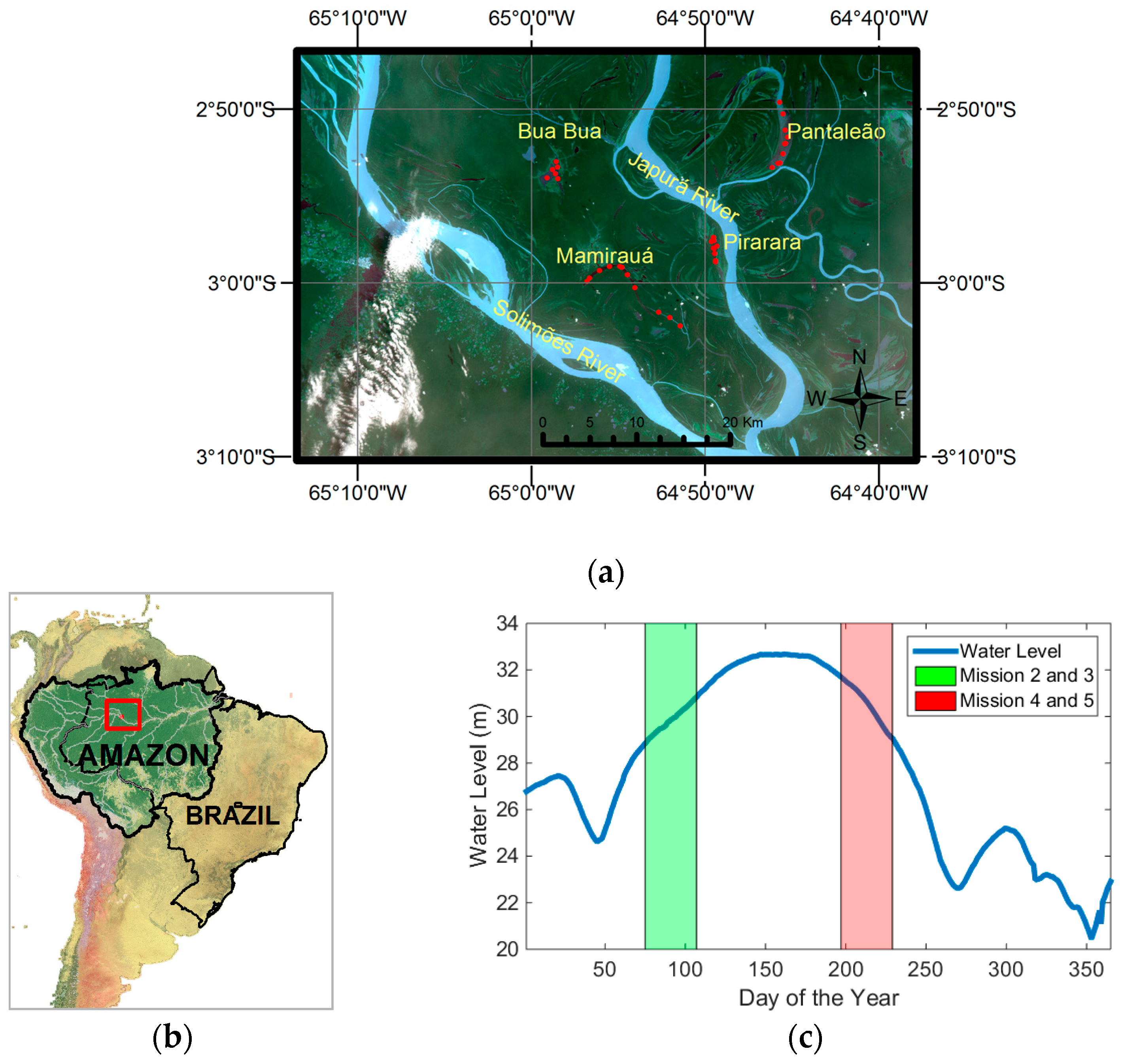
Figure 1.
(a) OLI true color image for the study area showing the selected lakes inside the MSDR. Red dots represent the distributions of points at each lake. The image is from December 4th of 2014. (b) Brazil figure with RDSM location evidenced in red (c) Hydrograph for the year 2016, showing water level variation for missions 2, 3 (in green) 4 and 5 (in red). Mission 1 occurred in the same flood phase as missions 4 and 5 in 2015.
Figure 2.
Rrs spectra for each lake in different water phases. (a) Mission 2 and 3 (rising water period); (b) Mission 1, 4, and 5 (receding water period). Each lake is represented by a specific color; Mamirauá in Blue, Bua-Buá in red, Pantaleão in green, and Pirarara in yellow.
Figure 2.
Rrs spectra for each lake in different water phases. (a) Mission 2 and 3 (rising water period); (b) Mission 1, 4, and 5 (receding water period). Each lake is represented by a specific color; Mamirauá in Blue, Bua-Buá in red, Pantaleão in green, and Pirarara in yellow.
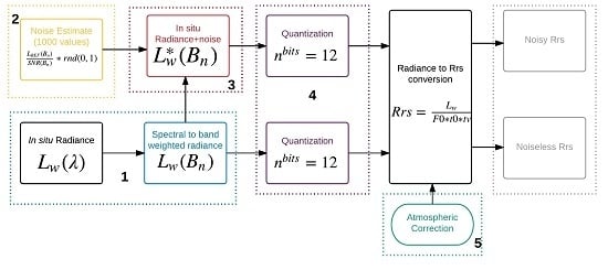
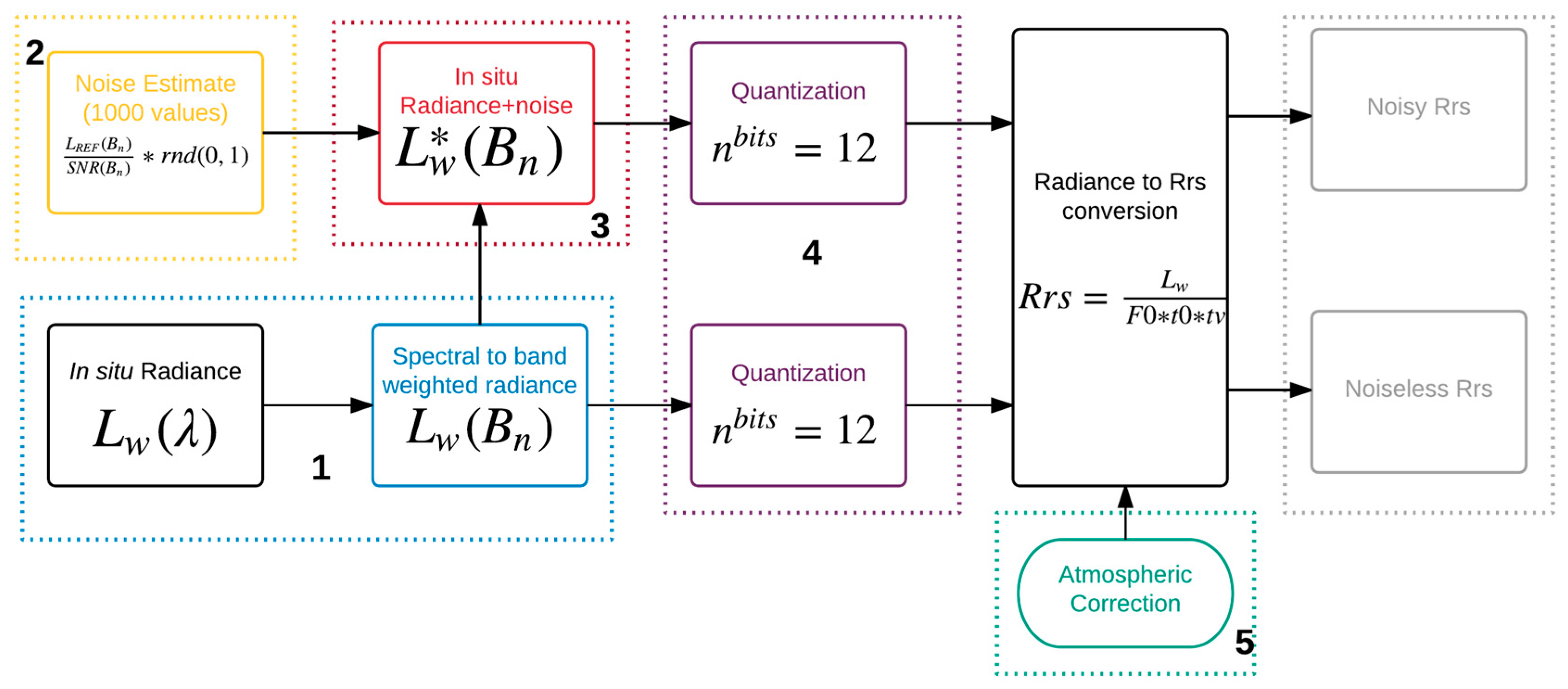
Figure 3.
Framework of the proposed simulation for a single spectrum of one orbital sensor.
Figure 3.
Framework of the proposed simulation for a single spectrum of one orbital sensor.
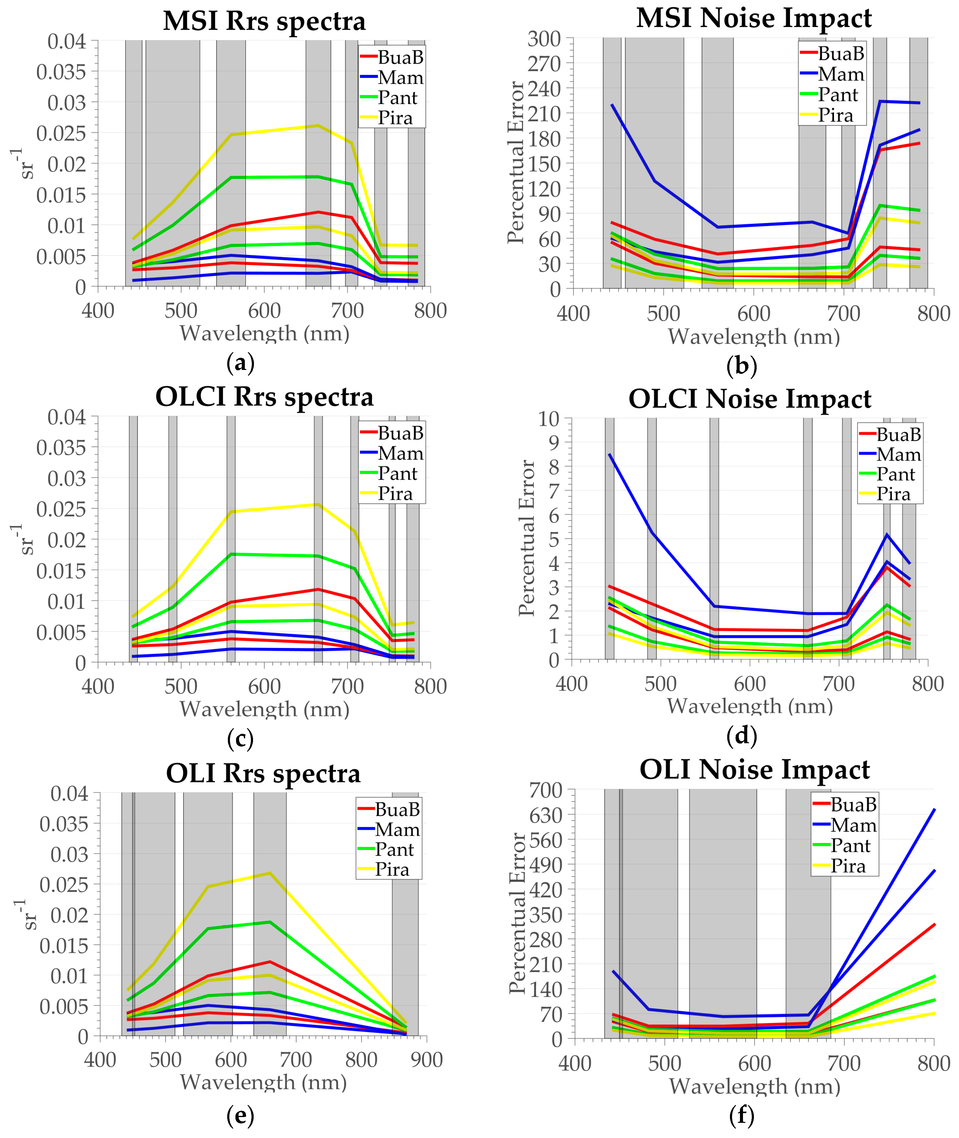
Figure 4.
(a–f) Noise band-weighted Rrs spectra for each sensor (a,c,e) and normalized error due to the optical characteristics of each sensor band (b,d,f), with two spectra of each lake. (a,b) MSI; (c,d) OLCI; (e,f) OLI. Each lake is represented by a specific color; Mamirauá in Blue, Bua-Buá in red, Pantaleão in green, and Pirarara in yellow. The noise used was equal to , in which rnd is the standard deviation of a standard normal distribution (equal to 1). The percent error is equal to .
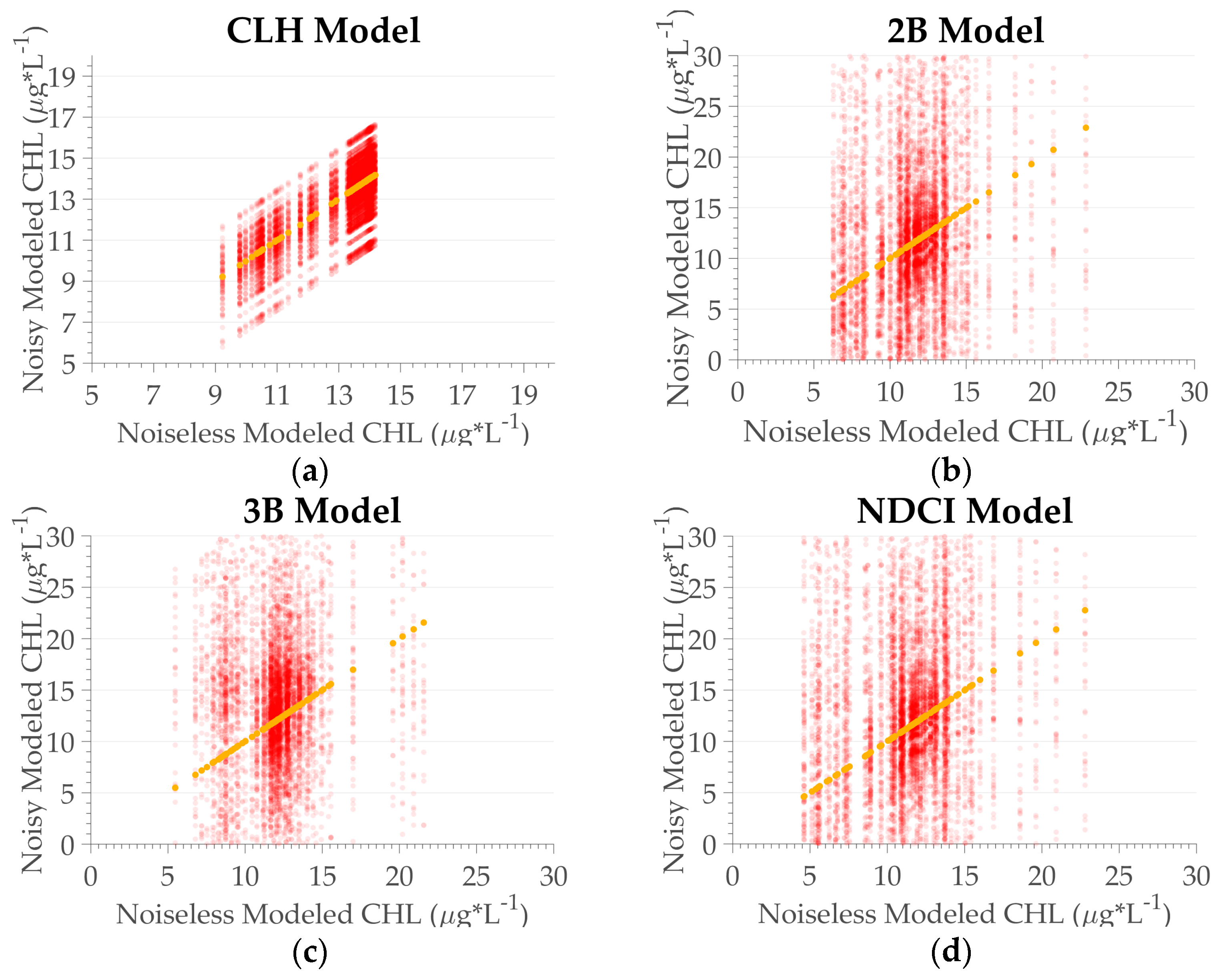
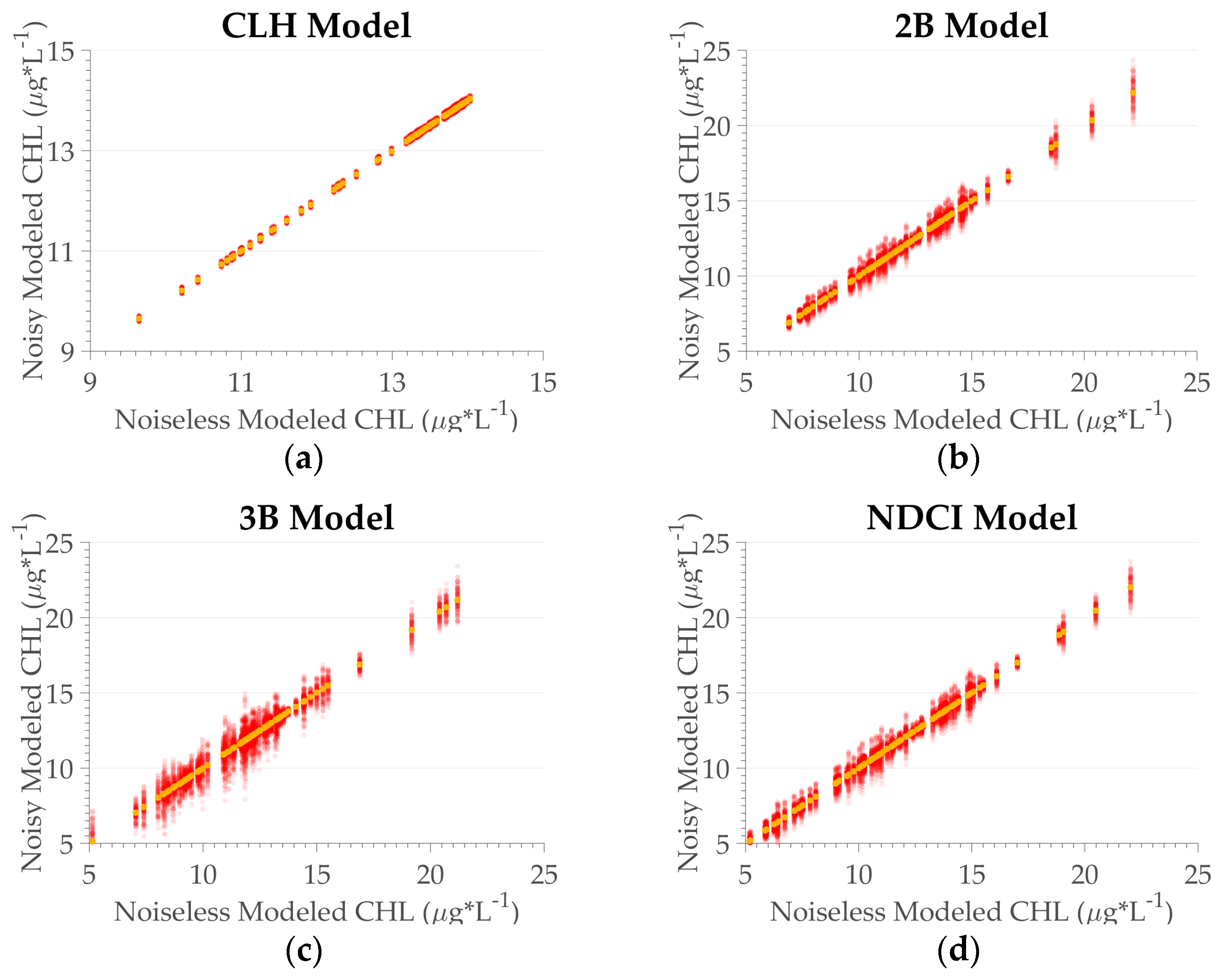
Figure 5.
Algorithm performance for the chl-a concentration of the MSI sensor. (a) CLH; (b) 2B; (c) 3B; (d) NDCI. Circles in red represent the data with noise, circles in yellow the noiseless data. The transparency is based on the frequency distribution, in which opaque indicates a higher frequency, and transparent indicates a lower frequency.
Figure 6.
Algorithm performance for the chl-a concentration of the OLCI sensor. (a) CLH; (b) 2B; (c) 3B; (d) NDCI. Circles in red represent the data with noise, circles in yellow the noiseless data. The transparency is based on the frequency distribution, in which opaque indicates a higher frequency, and transparent indicates a lower frequency.
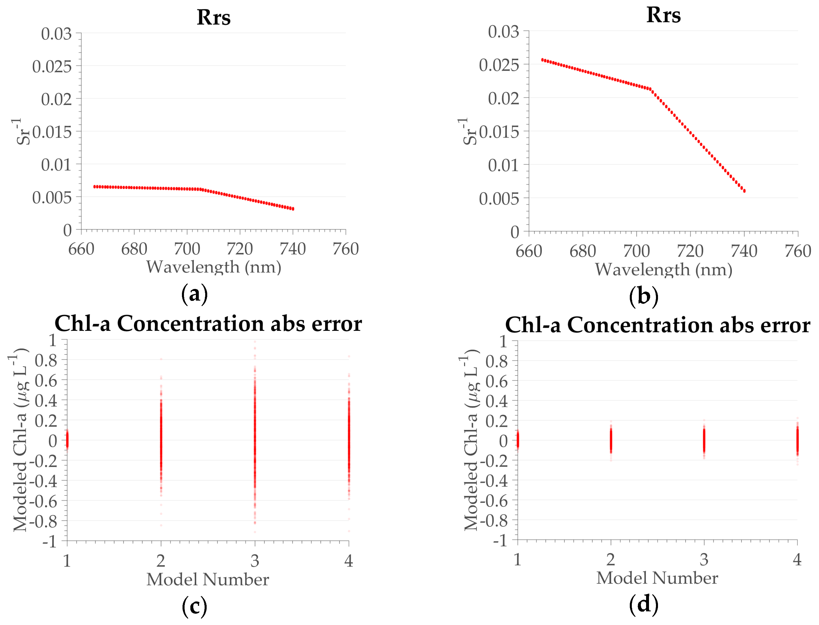
Figure 7.
Example of the OLCI Rrs magnitude and Chl-a concentration obtained for the four models for two lakes. (a) Rrs for three bands for one sample station of Bua-Buá, (b) Rrs for three bands for one sample station of Pirarara, (c) Chl-a concentration for the Bua-Buá sampling point, (d) Chl-a concentration for the Pirarara sampling point. The numbers 1, 2, 3, and 4 refer to the CLH, 2B, 3B, and NDCI models, respectively.
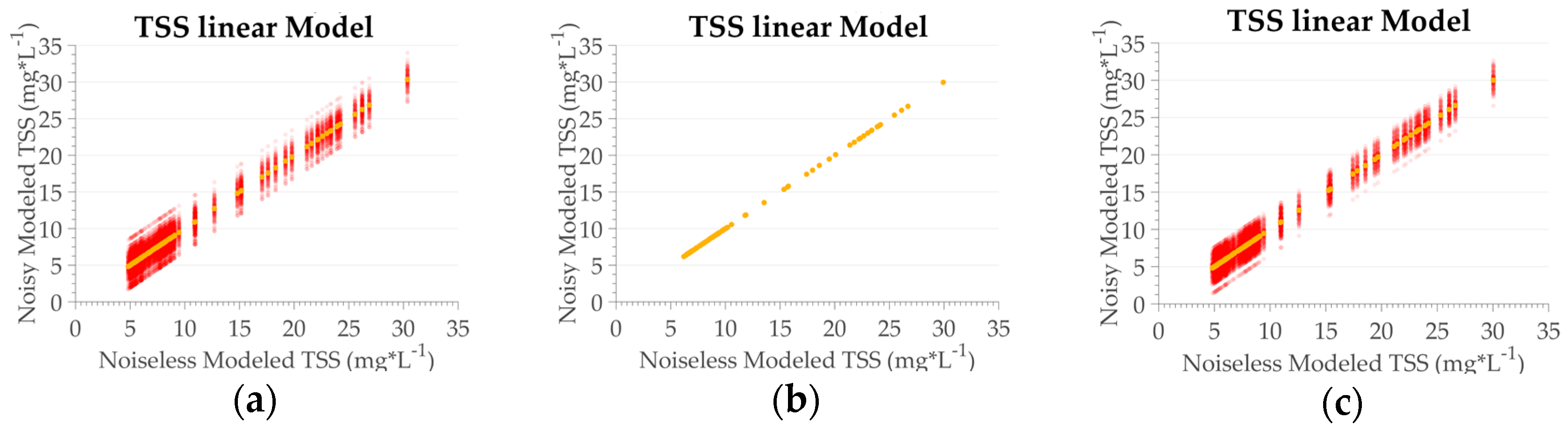
Figure 8.
TSS_linear model performance for TSS concentration. (a) MSI sensor; (b) OLCI sensor; (c) OLI sensor. Circles in red represent the data with noise, circles in yellow noiseless data. The transparency is based on the frequency distribution, in which opaque indicates a higher frequency, and transparent indicates a lower frequency.
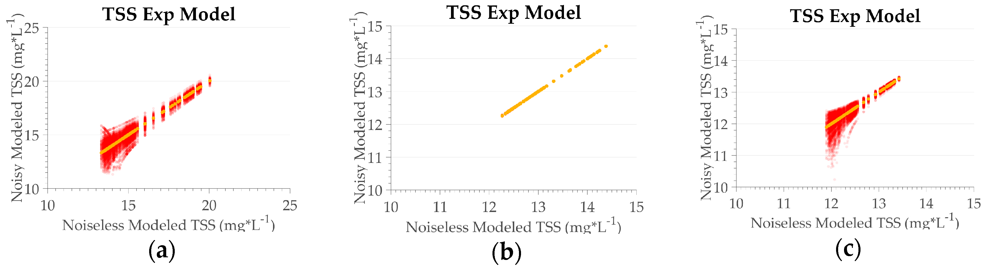
Figure 9.
TSS_exp algorithm performance for TSS concentration. (a) MSI sensor; (b) OLCI sensor; (c) OLI sensor. Circles in red represent the data with noise, circles in yellow noiseless data. The transparency is based on the frequency distribution, in which opaque indicates a higher frequency, and transparent indicates a lower frequency.
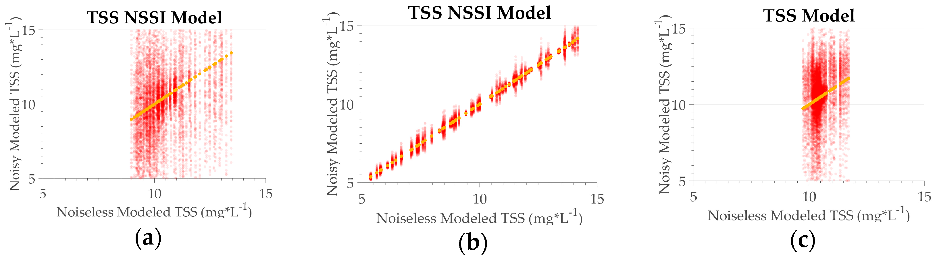
Figure 10.
TSS_NSSI algorithm performance for TSS concentration. (a) MSI sensor; (b) OLCI sensor; (c) OLI sensor. Circles in red represent the data with noise, circles in yellow noiseless data. The transparency is based on the frequency distribution, in which opaque indicates a higher frequency, and transparent indicates a lower frequency.
Table 1.
Limnological dataset for each lake and flooding phase. The names refer to the four lakes (Bua-Buá, Mamirauá, Pantaleão, and Pirarara). The mean value is shown followed by the standard deviation in parenthesis. Chl-a is Chlorophyll-a in µg/L, TSS is in mg/L, and is in m−1.
Table 1.
Limnological dataset for each lake and flooding phase. The names refer to the four lakes (Bua-Buá, Mamirauá, Pantaleão, and Pirarara). The mean value is shown followed by the standard deviation in parenthesis. Chl-a is Chlorophyll-a in µg/L, TSS is in mg/L, and is in m−1.
| | Rising Water | Receding Water |
|---|
| Bua | Mam | Pant | Pira | Bua | Mam | Pant | Pira |
|---|
| Chl-a | 14.7 (9.2) | 18.1 (6.2) | 11 (5.6) | 8.3 (3.4) | 8.2 (4.9) | 7.6 (4.7) | 12.1 (5.6) | 9.3 (3.6) |
| TSS | 9.5 (3.2) | 9.7 (2.6) | 18.5 (4.8) | 25.9 (6.8) | 5.5 (2.4) | 5.2 (1.1) | 7.5 (1.5) | 6.8 (1.3) |
| 5.6 (0.7) | 6.4 (1.5) | 2.1 (0.2) | 2.2 (0.2) | 2.5 (0.2) | 2.6 (0.3) | 2.5 (0.4) | 2.1 (0.2) |
Table 2.
MSI/Sentinel-2 sensor configurations used as the input for simulation. CW is the central wavelength (nm), BW is the band width (nm), SR is the Spatial Resolution (m), () is the radiance in which the SNR was calculated, Quant is the quantization, and () is the maximum radiance that can be measured by the sensor.
| Bands | CW | BW | SR | | SNR | Quant | |
|---|
| B1 | 443 | 20 | 60 | 129 | 129 | 12 | 588 |
| B2 | 490 | 65 | 10 | 128 | 154 | 12 | 615.5 |
| B3 | 560 | 35 | 10 | 128 | 168 | 12 | 559 |
| B4 | 665 | 30 | 10 | 108 | 142 | 12 | 484 |
| B5 | 705 | 15 | 20 | 74.5 | 117 | 12 | 449.5 |
| B6 | 740 | 15 | 20 | 68 | 89 | 12 | 413 |
| B7 | 783 | 20 | 20 | 67 | 105 | 12 | 387 |
Table 3.
OLCI/Sentinel-3 sensor configurations used as the input for simulation. CW is the central wavelength (nm), BW is the band width (nm), SR is the Spatial Resolution (m), () is the radiance in which the SNR was calculated, Quant is the quantization, and () is the maximum radiance that can be measured by the sensor.
| Bands | CW | BW | SR | | SNR | Quant | |
|---|
| B1 | 400 | 10 | 300 | 63 | 2188 | 12 | 413.5 |
| B2 | 412 | 10 | 300 | 74 | 2061 | 12 | 501.3 |
| B3 | 442 | 10 | 300 | 66 | 1811 | 12 | 466.1 |
| B4 | 490 | 10 | 300 | 51 | 1541 | 12 | 483.3 |
| B5 | 510 | 10 | 300 | 44 | 1488 | 12 | 449.6 |
| B6 | 560 | 10 | 300 | 31 | 1280 | 12 | 524.5 |
| B7 | 620 | 10 | 300 | 21 | 997 | 12 | 397.9 |
| B8 | 665 | 10 | 300 | 16 | 855 | 12 | 364.9 |
| B9 | 673 | 7.5 | 300 | 16 | 707 | 12 | 443.1 |
| B10 | 681 | 7.5 | 300 | 15 | 745 | 12 | 350.3 |
| B11 | 708 | 10 | 300 | 13 | 785 | 12 | 332.4 |
| B12 | 753 | 7.5 | 300 | 10 | 605 | 12 | 377.7 |
| B13 | 778 | 15 | 300 | 9 | 812 | 12 | 277.5 |
| B14 | 865 | 20 | 300 | 6 | 666 | 12 | 229.5 |
| B15 | 885 | 10 | 300 | 6 | 395 | 12 | 281 |
Table 4.
OLI/Landsat 8sensor configurations used as the input for simulation. CW is the central wavelength (nm), BW is the band width (nm), SR is the Spatial Resolution (m), () is the radiance in which the SNR was calculated, Quant is the quantization, and () is the maximum radiance that can be measured by the sensor.
| Bands | CW | BW | SR | | SNR | Quant | |
|---|
| B1 | 443 | 20 | 30 | 190 | 232 | 12 | 782 |
| B2 | 482 | 65 | 30 | 190 | 355 | 12 | 800 |
| B3 | 565 | 75 | 30 | 194 | 296 | 12 | 738 |
| B4 | 660 | 50 | 30 | 150 | 222 | 12 | 622 |
| B5 | 867 | 40 | 30 | 150 | 199 | 12 | 381 |
Table 5.
Parameters used during the conversion of the TOA irradiance solar spectrum to surface irradiance for all of the sensors.
Table 5.
Parameters used during the conversion of the TOA irradiance solar spectrum to surface irradiance for all of the sensors.
| Parameter | Range or Value |
|---|
| Date | 1 January |
| Time | 12 h 00 min (GMT) |
| Latitude | 0 |
| Ground Elevation | 40 m |
| Sensor Zenith Angle | 0 |
| Sensor Azimuth Angle | 0 |
| Ozone Amount | |
| Height of Maximum Ozone Concentration | 22 km |
| Atmopsheric pressure at site | 1014 |
Table 6.
Example of the parameters obtained and used during the atmospheric simulation for the MSI sensor. F0TOA is the band-weighted extraterrestrial solar irradiance, is the Rayleigh optical thickness for a standard atmosphere, and is the ozone optical thickness for 300 DU of atmospheric ozone.
Table 6.
Example of the parameters obtained and used during the atmospheric simulation for the MSI sensor. F0TOA is the band-weighted extraterrestrial solar irradiance, is the Rayleigh optical thickness for a standard atmosphere, and is the ozone optical thickness for 300 DU of atmospheric ozone.
| Band | | | |
|---|
| B1 (443) | 1938.2 | 0.2405 | 0.0004 |
| B2 (490) | 1916.5 | 0.1543 | 0.0087 |
| B3 (560) | 1845.9 | 0.0934 | 0.0309 |
| B4 (665) | 1524.7 | 0.0464 | 0.0167 |
| B5 (705) | 1402.5 | 0.0366 | 0.0063 |
| B6 (740) | 1290 | 0.0298 | 0.0030 |
| B7 (783) | 1184.8 | 0.0238 | 0.0002 |
Table 7.
Chl-a and TSS algorithms. The exact wavelength used changed for each sensor. CLH is a chlorophyll line height model, 2B is a red/NIR band ratio model, 3B is a red/NIR 3 band model, NDCI is a red NIR 2 band model, TSS_linear is a linear red band model, TSS_exp is an exponential red band model, and TSS_NSSI is a red/green exponential band ratio model.
| Model Name | Linear Model () | Reference |
|---|
| CLH | | [38] |
| 2B | | [39] |
| 3B | | [39] |
| NDCI | | [40] |
| TSS_linear | | [41] |
| | Non Linear model | Reference |
| TSS_exp | | [42] |
| TSS_NSSI | NSSI = ()/() | [43] |


 ,
, 


