A Radiometric Uncertainty Tool for the Sentinel 2 Mission

Abstract

In the framework of the European Copernicus programme, the European Space Agency (ESA) has launched the Sentinel-2 (S2) Earth Observation (EO) mission which provides optical high spatial resolution imagery over land and coastal areas. As part of this mission, a tool (named S2-RUT, from Sentinel-2 Radiometric Uncertainty Tool) has been developed. The tool estimates the radiometric uncertainty associated with each pixel in the top-of-atmosphere (TOA) reflectance factor images provided by ESA. This paper describes the design and development process of the initial version of the S2-RUT tool. The initial design step describes the S2 radiometric model where a set of uncertainty contributors are identified. Each of the uncertainty contributors is specified by reviewing the pre- and post-launch characterisation. The identified uncertainty contributors are combined following the guidelines in the ‘Guide to Expression of Uncertainty in Measurement’ (GUM) model and this combination model is further validated by comparing the results to a multivariate Monte Carlo Method (MCM). In addition, the correlation between the different uncertainty contributions and the impact of simplifications in the combination model have been studied. The software design of the tool prioritises an efficient strategy to read the TOA reflectance factor images, extract the auxiliary information from the metadata in the satellite products and the codification of the resulting uncertainty image. This initial version of the tool has been implemented and integrated as part of the Sentinels Application Platform (SNAP).

1. Introduction

Earth Observation (EO) via remote sensing nowadays provides one of the main sources of information about the Earth system. The complexity of many of these applications—land monitoring or climate studies—and the growing number of data sets, makes it increasingly necessary that this data has associated with it a quality indicator that describes the compatibility between different sensor data and the suitability for particular applications. Indeed the Committee on Earth Observation Satellites (CEOS) Working Group on Calibration and Validation (WGCV) through its Quality Assurance Framework for Earth Observation (QA4EO) explicitly states that data and derived products shall have associated with them an indicator of quality to enable users to assess the “fitness for purpose” of the data to their specific application [1]. Recent work described in [2] has resulted in the delivery of Sea surface temperature (SST) datasets with associated uncertainty estimates at a pixel level. The uncertainty estimates included in the SST products vary from 0.1 to 1.5 K, and they are largely dependent on the spatial and temporal distance with the satellite observations. This type of information is of a high-value to scientists working in climate models to understand the adequacy of the SST products for different observational conditions and is one example where the use of a single scene value for uncertainty could lead to misleading results. Similarly, where a user is interested in a particular localised area within a scene, unless pixel level uncertainty is available, they may not appropriately take account of potential adjacency effectives due to land cover types, coastal regions etc. and/or clouds etc.

The uncertainty provided in the EO products—Level-1 (L1) and higher—is the result of a chain that effectively links all the processing steps from the instrument down to the final product and that this chain should allow full traceability to the primary calibration through a measurement equation and account for any scene-dependent sensitivities. Ideally, TOA radiometric uncertainty provided with L1 EO products could be propagated through consecutive steps of the EO processing chain to higher level products, such as those describing biophysical parameters; through this process, uncertainties associated with L1 input parameters would effectively be one of the principle inputs to the higher‑level products’ uncertainty estimates. Furthermore, a rigorous uncertainty analysis of the L1 products may lead to a better understanding of the instrument and its radiometric performance by detecting systematic effects which may have been overlooked in previous analyses [3]. This assessment needs to consider the design of the sensor and how it makes and processes its measurements and establish a clear model which can allow any aspects that have scene-specific sensitivities. For example, detector noise, linearity, spectral characteristics, etc. can be evaluated with independent inputs and an appropriate uncertainty determined.

An example of the TOA radiometric uncertainty analysis can be found in [4]. The work proposes an uncertainty model combination and evaluates each one of the uncertainty contributions associated with the L1B algorithm of the reflectance solar bands of the Moderate Resolution Imaging Spectroradiometer (MODIS). This uncertainty resulted in an implementation of uncertainty images as part of MODIS L1B product [5,6].

The aim of this paper is to describe the efforts in designing and developing a tool and, more fundamentally, an exhaustive uncertainty analysis for the Sentinel-2 (S2) L1 mission products. The design and development of the tool has resulted in a first version of the tool implemented and released—S2-RUT (Sentinel-2 Radiometric Uncertainty Tool) [7]—that estimates the TOA radiometric uncertainties associated with each pixel using the S2 TOA reflectance factor images provided by the European Space Agency (ESA) as the input. The paper describes a method for the detailed analysis following the ‘Guide to Expression of Uncertainty in Measurement’ (GUM) [8] that can be easily adapted to other missions in the optical range. The uncertainty estimates provided by the tool can provide quality information to the users of L1 data—e.g., for instrument radiometric validation—and can be used as the input to propagate the uncertainty to higher-level products in a similar manner to that of the SST example described in [2].

The S2 mission has been recently launched by the ESA, in the framework of the European Union Copernicus programme, and is used for many applications, including urban planning, natural and man-made disasters management and crop monitoring. The research described in [9] and [10] shows a couple of the early applications of S2 data related to urban and crop monitoring, respectively. S2 incorporates as its main payload the MultiSpectral Instrument (MSI) which consists of 13 Visible and Near-InfraRed (VNIR) and Short-Wave InfraRed (SWIR) bands with spatial resolutions of 10 m, 20 m and 60 m as well as a short revisit time (5 days at the equator with two satellites) and a wide field of view (290 km) [11].

The MSI instrument uses an on-board sun diffuser, which is used nominally every month, to update the absolute radiometric calibration and the relative gains calibration. There is no secondary diffuser on-board for checking the degradation of the calibration diffuser and, thus, it relies on a pre-determined optimised exposure based on heritage knowledge and monitoring through vicarious and cross-mission validation using terrestrial sites. Every two weeks, images acquired over ocean at night are used to update the dark signal calibration [11].

The structure of the paper follows the same logic applied in the design and development process of the S2-RUT tool. The first part of the design takes into account the S2 radiometric model, described in Section 2, and identifies each of the uncertainty contributors, described in Section 3, and links them to the parameters in the L1 processing model. Effort has been put into an exhaustive specification and assessment of each contributor by reviewing the results of the pre- and post-launch characterisation. The identified uncertainty contributors are combined following the guidelines in the GUM [8]. Particular attention has been given to the validation and exhaustive discussion of the uncertainty combination method in Section 4. The software design of the tool has emphasised the use of computationally efficient strategies to read the TOA reflectance factor images and is discussed in Section 5. Effort has been made in the automatisation of the uncertainty evaluation to include the option to extract the auxiliary information from the metadata in the satellite products. The first version of the tool also includes the assessment of the uncertainty at a desired coverage probability by setting a coverage factor, k, and the selection/deselection of the uncertainty contributors for sensitivity studies. This initial version of the tool has been implemented—code available at [7]—and integrated as part of the Sentinel Application Platform (SNAP) [12]. The first version of the tool is referred to in this paper as S2-RUTv1. This first version focuses on describing in detail an exhaustive uncertainty methodology and a general software design that can form the basis of adoption to several other EO missions. The tool is open to the community and is under continuous evolution, with the expectation that future versions will include a refined uncertainty assessment and/or new tool features.

The S2-RUT provides uncertainty estimates and, to avoid any potential misunderstandings, we feel it is useful to clarify the terminology. Firstly, error is the discrepancy between the measured value and the quantity intended to be measured. This error can be the result of random effects that produce variations in each observation and systematic effects which can be known and corrected for or that respond to an incomplete knowledge of the quantities measured. By contrast, uncertainty expresses the degree of doubt around the measured value. The uncertainty is the evaluation of the impact of the random and systematic effects associated with the error. The uncertainty is not necessarily an indication of the likelihood that the measured value is near the quantity to be measured. It responds to an estimation of the likelihood of approximation to the measured value that is consistent with presently available knowledge. Thus, it is possible that systematic effects may have not been identified and consequently corrected or assessed due to lack of knowledge. In terms of probability, the uncertainty refers to an interval about the result of a measurement that may be expected to encompass a certain fraction of the distribution of values that could reasonably be attributed to the quantity to be measured. The coverage factor, k, is a numerical factor used as a multiplier of the combined standard uncertainty in order to specify the fraction of the probability distribution that the uncertainty represents. The expanded uncertainty is the result of the multiplication of the combined standard uncertainty by the coverage factor [8].

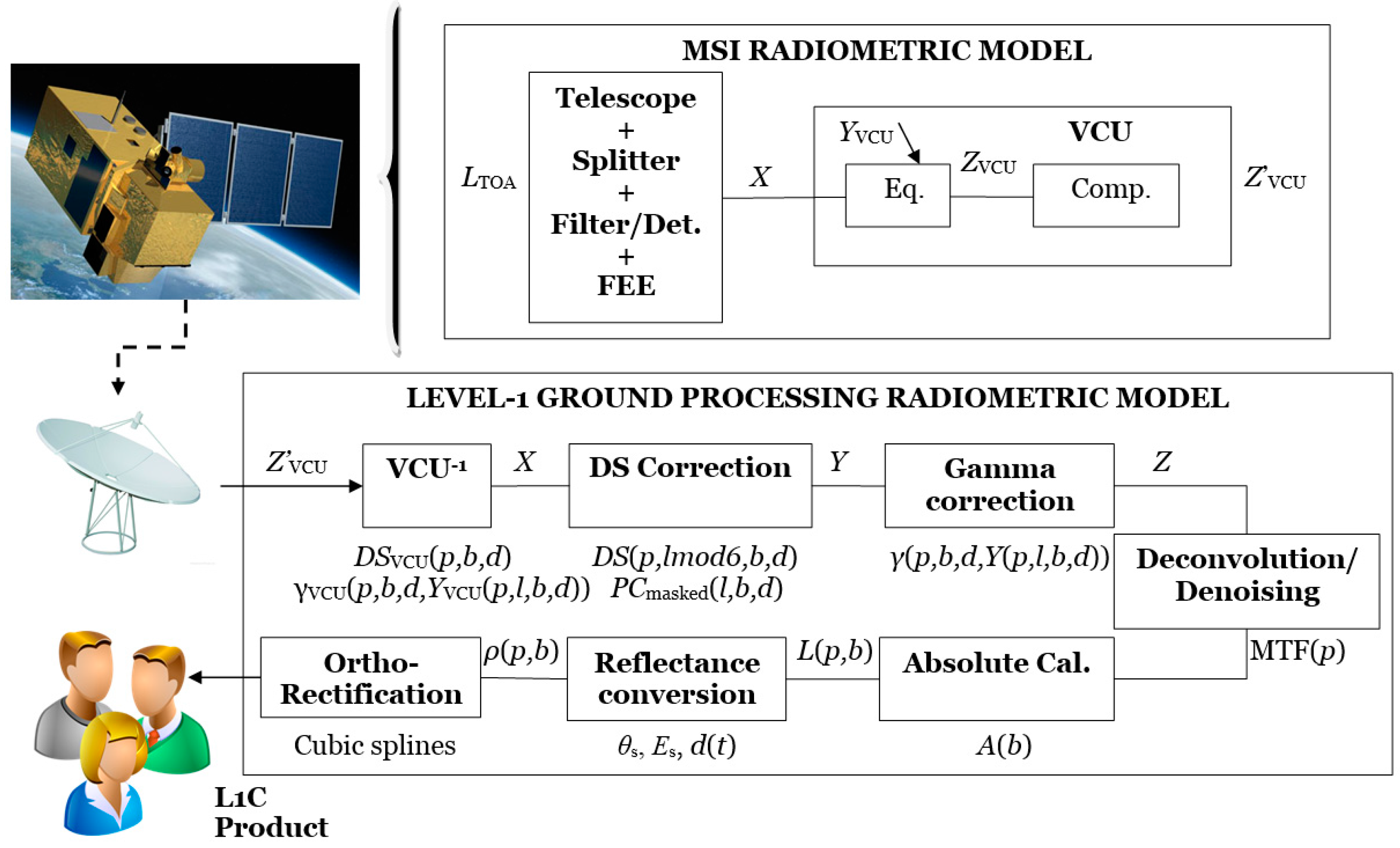
2. Sentinel 2 Level-1 Radiometric Model

The first step in any radiometric uncertainty analysis is, where possible, to identify the mathematical equation that describes the data processing at each step of the chain. The description of the Sentinel-2 mission and L1 processing can be found in [13,14]. Figure 1 illustrates the MSI instrument acquisition and L1 processing. In the graph, the parameters p, l, b and d correspond to the selected pixel, line, band and detector respectively.

The MSI instrument collects the incoming radiance (L_TOA) through a three-mirror off-axis anastigmatic telescope. The incoming light is separated at the splitter into visible and near-infrared (VNIR) and short-wave infrared (SWIR). This light is filtered and detected at the instrument focal plane. At the output of the front-end electronics (FEE), the raw signal, X, is pre-equalised and compressed—boxes “Eq.” and “Comp.” in Figure 1—by the video chain unit (VCU) and the signal Z’_VCU is sent down to Earth. Once the signal is received, a decompression (VCU⁻¹) is executed. This process is assumed deterministic and for simplification is not included in the mathematical model.

The radiometric standard correction model for the Sentinel-2 L1B (geolocated pixels with counts proportional to Earth radiances) product is presented in [14]:

$$\begin{array}{l}Y(p,l,b,d)=X(p,l,b,d)-DS(p,l\mathrm{mod}6,b,d)-P{C}_{\mathrm{masked}}(l,b,d)\\ Z(p,l,b,d)=\gamma (p,b,d,Y(p,l,b,d))\end{array},$$

(1)

where Y(p,l,b,d) is the raw signal X(p,l,b,d) of pixel p corrected to allow for the dark signal DS(p,lmod6,b,d) and the pixel contextual offset, PC_masked(l,b,d), expressed in Least Significant Bit (LSB); γ(p,b,d,Y(p,l,b,d)) is a function that compensates for the non-linearity of the global response of the pixel p and its relative behaviour with respect to other pixels; Z(p,l,b,d), is the equalised signal after relative and non-linear correction (in LSB); and DS(p,j,b,d) is the dark signal of the pixel p in channel b for chronogram sub-cycle line number j (j is in the range 1 to 6).

The initial quantisation produced at the instrument in order to digitise the analogue output of the instrument is as follows:

$$X(p,l,b,d,L(\lambda ))=\mathrm{trunc}\left[G(p,b,d,L(\lambda ))\cdot V(p,l,b,d,L(\lambda ))\right],$$

(2)

where G(p,b,d, L(λ)) represents the gain of the pixel p in channel b and detector d at the video chain and V(p,l,b,d, L(λ)) is the voltage recorded for the input radiance, L(λ).

The pixel contextual offset, PC_masked, parameter aims to compensate for the dark signal variation due to voltage fluctuations in-orbit. It is described by:

$$P{C}_{\mathrm{masked}}(l,b,d)=\frac{1}{N_{\mathrm{masked}}}\cdot {\displaystyle \sum _{i=1}^{N_{\mathrm{masked}}(b)}[X(i,l,b,d)-DS(p,l\mathrm{mod}6,b,d)}],$$

(3)

where DS(p,j,b,d) is the dark signal of the pixel p in channel b, for chronogram sub-cycle line number j, N_masked(b) is the number of masked pixels on both sides of the detector line for channel b and mod is the “modulo” function.

The relative gains, γ(p,b,d,Y(p,l,b,d)), correct for the non-uniformity and non-linearity of the pixels and codify them in an unsigned two-byte integer. The formulation is presented below for the VNIR bands (left) and the SWIR bands (right):

$$\begin{array}{l}Z=\mathrm{round}[G0+G1\cdot Y+G2\cdot Y^2+G3\cdot Y^3]\mathrm{if}Y\ge 0\\ Z=0\leftrightarrow Y<0\end{array}\begin{array}{l}Z=0\leftrightarrow Y\le Z_C\\ Z=\mathrm{round}[A1\cdot (Y-Z_C)]\mathrm{if}{Z}_C<Y\le Z_C+Z_S\\ Z=\mathrm{round}[A2\cdot (Y-Z_S-Z_C)+A1\cdot Z_S]\mathrm{if}Y>Z_C+Z_S\end{array}$$

(4)

The coefficients G0, G1, G2 and G3 correspond to a cubic polynomial whereas the coefficients A1, A2, Z_S and Z_C correspond to the coefficients of a double linear fitting equation. These values have been characterised pre-flight and are monitored in-flight by the diffuser acquisitions on a monthly basis. If the variation is sufficiently large, the curves are re-scaled as follows:

$${\gamma }_{\mathrm{updated}}(p,b,d,Y)={\gamma }_{\mathrm{ground}}(p,b,d,\frac{{\gamma }_{\mathrm{ground}}{}^{-1}(p,b,d,\overline{Z_{\mathrm{sd}}(p,b,d)})}{Y_{\mathrm{sd}}(p,b,d)}\cdot Y),$$

(5)

In order to obtain the L1C (orthorectified reflectance factor) product, the native pixels are re-sampled in a two-step process. First, a geometric process computes the grid that gives, for each point of the output image, its location in the focal plane and a bi-spline interpolation function calculates the radiometric quantity in the output image [13]. The result provides an orthorectified image where CN_k,NTDI(i,j) is the equalised numeric digital count of the pixel (i,j) for the band k and NTDI, is the Number of Time Delay Integration lines. The parameters k and b represent both the MSI spectral bands but at L1C and L1B processing chains, respectively. That is, k refers to the spectral band of the orthorectified image, whereas b refers to the spectral band of the instrument focal plane image.

As a final step, the digital counts CN_k,NTDI(i,j) are converted into reflectance factors (TOA reflectance normalised to the ideal Lambertian diffuser):

$${\rho }_k(i,j)=\frac{\pi \cdot C{N}_{k,\mathrm{NTDI}}(i,j)}{A_{k,\mathrm{NTDI}}\cdot E_{\mathrm{S}}\cdot d(t)\cdot \cos ({\theta }_{\mathrm{S}}(i,j))},$$

(6)

where E_S is the equivalent extra-terrestrial solar spectrum and depends on the spectral response of the S2 bands, d(t) is a correction for the Sun−Earth distance variation, A_k,NTDI is the absolute calibration coefficient, and θ_S(i,j) is the per-pixel Solar Zenith Angle (SZA). The value of A_k,NTDI is described as:

$$A(b)=\frac{1}{N_p\cdot N_l\cdot N_d}\cdot {\displaystyle \sum _{p,l,d}\frac{\pi \cdot d_{\mathrm{sun}}^2\cdot Y_{\mathrm{sd}}(p,l,b,d)}{K_{\mathrm{slt}}\cdot \rho (p,{\theta }_{\mathrm{sd}}(l),{\phi }_{\mathrm{sd}}(l))\cdot E_{\mathrm{sun}}(b)\cdot \cos {\theta }_{\mathrm{sd}}(l)}},$$

(7)

where K_slt refers to the stray-light correction in calibration, N_l refers to the number of averaged lines l, and θ_sd, ${\phi }_{\mathrm{sd}}$ are the SZA and Viewing Zenith Angle (VZA) of the diffuser, respectively.

The parameter d(t) does not directly account for the inverse square law of irradiance. The parameter d(t) already accounts for the square relationship with the Sun−Earth distance variation and this effect has been inverted. The relationship is as follows:

$$d(t)=\frac{1}{{\left(1-0.01673\cdot \cos (0.0172\cdot (t-2)\right)}^2},$$

(8)

3. Radiometric Uncertainty Contributions

3.1. Uncertainty Contributions: Identification

From the radiometric equations presented in Equations (1)–(8), it is possible to identify the main sources of uncertainty and the sensitivity coefficients for each one of them.

Table 1. List of Sentinel-2 L1 radiometric uncertainty contributions and their associated parameter in the radiometric processing model. The table also indicates the contributions that are considered for the S2-RUTv1 implementation (marked as “Y”), the ones that may be included in next versions of the tool (marked as “N”) and the ones that have a negligible effect (i.e., <0.1%).

L1B Contributor	Parameter	S2-RUTv1	L1C Contributor	Parameter	S2-RUTv1
Instrument noise, unoise	X(p,l,b,d)	Y	Diffuser reflectance absolute knowledge, udiff_abs	ρsd(p,θsd(l), ${\phi }_{\mathrm{sd}}$(l))	Y
Out-of-field Stray-light—systematic part, ustray_sys	X(p,l,b,d)	Y	Diffuser reflectance temporal knowledge, udiff_temp	ρsd(p,θsd(l), ${\phi }_{\mathrm{sd}}$(l))	Y
Out-of-field Stray-light—random part, ustray_rand	X(p,l,b,d)	Y	Angular diffuser knowledge—BRF effect	ρsd(p,θsd(l), ${\phi }_{\mathrm{sd}}$(l))	<0.1%
Crosstalk, ux_talk	X(p,l,b,d)	Y	Instrument noise and dark signal during calibration	Ysd(p,l,b,d)	<0.1%
Deconvolution residual	X(p,l,b,d)	N	Solar irradiance model	ES(b)	<0.1%
Polarisation error	X(p,l,b,d)	N	Angular diffuser knowledge—cosine effect, udiff_cos	cos(θsd(l))	Y
ADC quantisation, uADC	X(p,l,b,d)	Y	Straylight in calibration mode—residual, udiff_k	Kslt	Y
Compression noise	X(p,l,b,d)	<0.1%	Sun-to-satellite distance knowledge	d(t)	<0.1%
Dark signal knowledge	DS(p,j,b,d)	<0.1%	Angular observation knowledge—cosine effect	cos(θS(i,j))	<0.1%
Dark signal stability, uDS	PCmasked(l,b,d)	Y	Orthorectification uncertainty propagation	ρk(i,j)	N
Non-linearity and non-uniformity knowledge, ugamma	γ(p,b,d,Y)	Y	Spectral knowledge	ρk(i,j)	N
Non-uniformity spectral residual	γ(p,b,d,Y)	N	Geometric knowledge	ρk(i,j)	N
L1B Image quantisation	CNk,NTDI(i,j)	<0.1%	L1C Image quantisation, uref_quant	ρk(i,j)	Y

identifies each of the uncertainty contributions and links them to the parameters in Equations (1)–(8). The table also clarifies the contributions which are included in the S2-RUTv1 as well as the ones that have a negligible impact and the ones that are expected to be included in further versions of the tool.

The general criteria to qualify the contributors as negligible is that they have an impact of <0.1 DN or <0.1%. The term Solar irradiance model is the exception to this rule. It has been classified as negligible and is indeed not included in the budget since the reflectance factor cancels its effect. The Sun irradiance model applied is the one described in Thuillier et al. [15]; this is used for both the absolute calibration calculation in Equation (7) and the reflectance factor conversion in Equation (6). However, if the product were to be converted into radiance, the uncertainty in the solar irradiance model should be included and would definitely not be negligible. A description of the estimated uncertainty for the solar model is provided in [15].

The following lists the negligible uncertainty contributions from Table 1 with a brief description of why these have been deemed negligible:

• The dark signal knowledge is well known to be below the 0.1 DN level as a consequence of the averaging of several hundreds of samples. If the samples are fully uncorrelated, the standard deviation of the mean describes the associated uncertainty. When this is not the case, alternative methods such as the Allan deviation have been described and applied to the S2 dark datasets in [16]. In that case, it was demonstrated how hundreds of samples can be considered as independent in the dark dataset for most of the pixels and bands. Thus, the averaging of hundreds of samples reduces the noise by a factor well above 10.
• The compression noise has been optimised so that N_total ≤ 1.2 NeDL. Here N_total refers to the instrument and compression noise and NeDL refers to the noise equivalent radiance without compression noise. The effect is thus limited to a worst-case situation of 20% of total noise level. The MSI instrument specifications for signal-to-noise ratio (SNR) are generally at L_ref and are typically between 100 and 200 for most of the bands. The term L_ref denotes the reference radiance for the MSI design and can be found in [11]. The compression noise is thus a contribution that in most of the scenarios can be assessed as <0.1%. Nonetheless, this might not be true for specific cases—e.g., low radiance measurements. For example, setting the worst-case situation with an SNR of just 50 and worst-case compression rate (N_total = 1.2 NeDL), the error could scale up to 0.4%. Future versions of the tool will consider more specific cases by monitoring the compression rates.
• The L1B image quantisation has a minimum impact since the ground processing uses a double datatype (i.e., 32 bits).
• The Angular diffuser knowledge—BRF effect. The vibrations and diffuser creeping limit the knowledge of the angular coordinates during calibration. This effect has a minimum impact in the BRF assessment due to the near-Lambertian shape of the diffuser on-board together with a low angular uncertainty. The same reasoning does not apply for the cosine correction and is further explained in Section 3.2.10.
• The Instrument noise and dark signal during calibration is well known to be below the 0.1% level. Similar reasoning as for dark signal knowledge can be inferred here. Even for a SNR of 50 as specified for B10 in [11], averaging over just 400 independent samples would reduce the noise below the 0.1% level.
• The Sun-to-satellite distance knowledge should have a negligible impact since the positioning of the satellite with respect to the Sun—which involves the Sun and Earth ephemeris, as well as satellite positioning—is declared to be known without significant error.
• The Angular observation knowledge—cosine effect is well known again because of the correct positioning of the satellite with respect to the Sun. In calibration mode, the micro-vibrations and diffuser creeping affect the diffuser coordinate system but does not affect the Earth surface and Sun positioning. Note that this tilting—e.g., micro-vibrations of the satellite, orbit precision, etc.—is accounted for in the Geometric knowledge contribution.

The contributors that are not included in S2-RUTv1, marked as “N” in Table 1, are expected to be assessed in future iterations of the tool. These contributions represent a challenging assessment and are subject to interpretation. That is, several of them have a strong dependency on the TOA spectral characteristics of the scene under measurement, whereas others largely depend on the neighbouring pixels. For example, the “spectral knowledge” will largely depend on the spectral signature of the measured scene whereas the uncertainty propagation through the orthorectification and the accuracy of the resampling will depend on the radiometric uniformity of the scene. The “novel methodologies” required to assess these contributors have already been discussed in [17] which provides a preliminary discussion of the impact of the Ortho-rectification uncertainty propagation and Spectral knowledge. The refinement of these methods might result in the implementation of these contributors in further versions of the S2-RUT. Here they are briefly described:

• Deconvolution residual. The signal deconvolution and denoising are considered for its compensation during the ground processing. The residual of this correction—so far not assessed—would represent the uncertainty to be included in the budget (deconvolution and denoising stages in Figure 1). This effect would take into account the Point Spread Function (PSF) dispersion by the mirror scattering but also the potential correction of ghosting effects in the across- and along-track. Although all these contributions are similar in nature, they should not be confused with the out-of-field stray-light—systematic part (described at Section 3.2.2), the out-of-field stray-light—random part (described at Section 3.2.3) and the optical crosstalk (described at Section 3.2.4).
• Polarisation error. This is considered not to be a major source of error for land measurement and is not corrected for during the ground processing—the polarisation sensitivity of the MSI instrument is <3% and the degree of polarisation (DoP) is generally <10% for most land measurements. Note, however, that for specific cases, the DoP could be above 10%—e.g., inner water and coastal measurements. For those cases, the error should be flagged and, if necessary, corrected as discussed in [16].
• Non-uniformity spectral residual. The relative gains are updated in-flight by measuring the solar illumination-reflected from the diffuser. The disagreement of the Sun spectral signature with respect to the nominal measurements of the Earth-reflected light introduces a systematic effect. A potential method to assess this uncertainty contributor could follow a similar methodology as for Landsat-8 Operational Land Imager (OLI) [18].
• The Ortho-rectification uncertainty propagation, involves the radiometric interpolation of the input data to transform the MSI focal plane measurements to a pre-defined grid on the Earth. Recent missions, such as S2, include a bi-spline interpolation of the data. Research in [17] has proposed a preliminary implementation of the propagation of the uncertainty through the resampling process. Further assessment should also consider the accuracy of the resampling with respect to the real scene fluctuations.
• The Spectral knowledge is produced as a consequence of the limited knowledge of the pre-flight spectral calibration and the subsequent post-launch variations. The pre-flight spectral knowledge is ultimately limited by the alignment and spectral characteristics of the calibration source. The post-launch variations are produced due to in-orbit temperature variations or temporal degradation, among others. In addition, the spectral response is typically associated with the mean for all the pixels across the focal plane. The residual of this effect is accounted in Non-uniformity spectral residual contributor. See [17] for the preliminary assessment and first implementation of this contributor.
• The geometric knowledge referred to here is the impact that the geometric uncertainty has in the radiometry. That is, how limitations in the pointing and the geo-location of the sensor can lead to error in the resultant products; this will be directly dependent on the degree of radiometric non-uniformity and the size of the scene being viewed. The nature of the effect will depend on whether the user requires a single pixel measurement or a larger area, since this effect will be largely correlated in the spatio-temporal domain.

There are 12 uncertainty contributors which have been considered for the initial version of the S2-RUTv1. Each one of them will be presented separately at the different sub-sections in 3.2.

3.2. Uncertainty Contributions: Description and Assessment

3.2.1. Instrument Noise

The S2 L1C product includes, as part of the metadata, the parameters α_Z and β_Z of a noise model evaluated and updated in-flight using the dark signal and diffuser measurements [19]. The two parameters and the noise model are defined at pixel level as:

$$\begin{array}{l}Nois{e}_Z(p,l,b,d)=\sqrt{{\alpha }_Z{(p,l,b,d)}^2+{\beta }_Z(p,l,b,d)\cdot Z(p,l,b,d)}\\ {\alpha }_Z(p,l,b,d)=ST{D}_l[Z_{\mathrm{ds}}(p,l,b,d)]\\ {\beta }_Z(p,l,b,d)=\frac{ST{D}_l^2[Z_{\mathrm{sd}}(p,l,b,d)]-{\alpha }_Z{(p,l,b,d)}^2}{A(b)\cdot K_{\mathrm{slt}}\cdot \frac{1}{N_l}\cdot {\displaystyle \sum _l\frac{\rho (p,{\theta }_{\mathrm{sd}}(l),{\phi }_{\mathrm{sd}}(l))}{\pi }\cdot }\frac{E_{\mathrm{sun}}(b)}{d_{\mathrm{sun}}^2}\cdot \cos {\theta }_{\mathrm{sd}}(l)}\end{array},$$

(9)

where Z_ds(p,l,b,d) and Z_sd(p,l,b,d) are the equalised signals—as defined in Equation (1)—for the dark and diffuser measurements, respectively, and STD is the standard deviation operator. Other symbols are as previously defined in Section 2.

The noise model takes the DS standard deviation (α_Z) as the instrument noise in the absence of light and scales it by the signal measured. The scaling factor relies on the assumption that the increase of the noise with the light intensity is produced by the photon shot noise and is linear with respect to the variance (STD²).

Note that the dark and diffuser samples are taken at a different part of the orbit and thus requires the assumption that minimum noise drift—e.g., as a consequence of voltage or temperature variations—occurs during the orbit.

The S2 noise has been modelled pre-flight using a more complex model with estimations at the beginning and end of life and a per-pixel cubic fitting. This semi-empirical model relies on a complex characterisation where apart from variance estimations at different radiance levels, other noise linearity effects such as the sense node capacitance are included. However, the pre-flight model will not be used for noise estimation since it cannot be updated in-flight and the assignment of noise coefficients at pixel level requires a large memory.

Thus, calculating the noise by reading the values α and β which are appended to the product metadata is a simple but effective approach since it minimises the computing requirements and it is continuously updated during the mission lifetime and during any potential dataset re-processing.

The previous work in [16] showed how the dark noise standard deviation (α parameter) was not changing significantly across the sensor array. It was ultimately limited by the Poisson distribution with approximate changes of ±0.1 LSB. Nonetheless, for specific cases, the pixels present characteristic “dark spikes” of noise much higher than the rest of pixels and are typically named “hot pixels.” Note that these are not invalid pixels but pixels, for example, with different levels of impurities to other ones [20]. These specific cases should be flagged and potentially reported to account for in future versions of the tool.

3.2.2. Out-of-Field Stray-Light Systematic Part

This contribution refers to the out-of-field stray-light measured during nominal Earth observation that is not measured during calibration due to different angular configuration. This effect of the Earth out-of-field stray-light has been analysed as 0.3%∙of L_ref and verified by measurements using a uniform source out of the FOV.

Contrary to the stray-light in calibration mode described in Section 3.2.11, this effect is not currently corrected for in the L1 processing chain. Thus, this contributor is a known systematic effect (i.e., error) and not an uncertainty contributor (see [8]).

The error correction would apply an offset term to the absolute calibration, as shown by rearranging Equation (6):

$${\rho }_k(i,j)=\frac{\pi }{E_{\mathrm{S}}\cdot d(t)\cdot \cos ({\theta }_{\mathrm{S}}(i,j))}\cdot \left(\frac{C{N}_{k,NTDI}(i,j)}{A_{k,NTDI}}-0.003\cdot L_{\mathrm{ref}}\right),$$

(10)

Using a constant level of 0.3%∙L_ref assumes that the out-of-field stray-light comes uniformly from the whole Earth whereas it is more likely that the effect will be higher for parts of the scene closer to the limits of the FOV limits. Thus, the correction would have associated variations that define the knowledge of the correction and should be accounted for in the uncertainty residual.

Although the GUM recommends that corrections for known significant systematic effects must be applied to measurement results, this may not always be feasible in specific cases such as here. Since at the time of writing this effect has not been corrected for, then for the development of the S2-RUTv1, the guideline in [8] (note on 6.3.1, p. 24) has been applied. It means that this contributor will “enlarge” the expanded uncertainty estimate by adding this component linearly—see Section 4.1 and Section 4.2.

3.2.3. Out-of-Field Stray-Light Random Part

This contribution is the result of the “undesired light” that scattered into the focal plane. During the prelaunch tests of light tightness, a small fraction of light was detected at VNIR focal plane. No light was detected at the SWIR focal plane.

In terms of uncertainty, this is modelled as a normal distribution due to its random nature across the detector array. Nonetheless, this modelling is to be reconsidered in further revisions of the S2-RUT for two reasons:

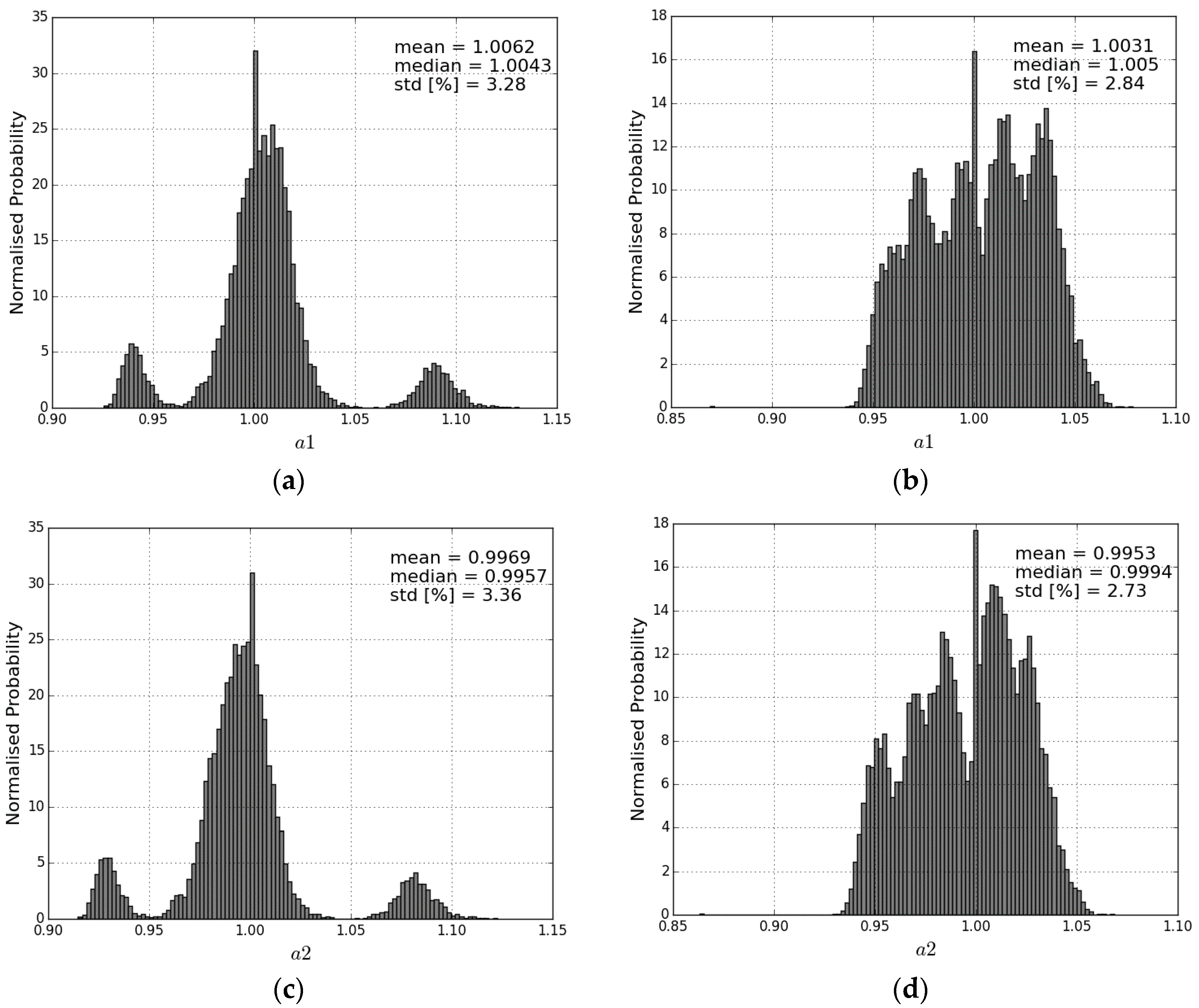
• The assumption of a normal distribution has not been verified. There is the possibility that this distribution actually approaches a rectangular one rather than normal.
• The effect is systematic at a pixel level. That is a similar offset will be expected independently of the scene for a specific pixel. The modelling as a distribution refers to the impossibility to know a specific offset at a pixel level.

3.2.4. Crosstalk

The crosstalk is subdivided into the optical and electrical effects.

The optical channel crosstalk is produced by the internal reflection between filters and detectors. As a consequence, some rays intended for a specific detector array are incident on a different detector array. Through a thorough design effort, the inter-reflections have been reduced to a negligible level.

The contributions for the electrical crosstalk arise from the detectors, the on-board electronics, and the video chain. The assessment has identified all the sources of “contamination” from one band and studied the worst case. The effect is low for the VNIR channels even at very low radiance levels, while the effect is relatively important for the SWIR bands where the detector electrical crosstalk is significant when expressed in relative terms.

This contribution is indeed a systematic effect that could be corrected for at the focal plane measurement level. For the initial version of the tool, a pragmatic approach has been utilised—the worst-case values have been used as uncertainty estimates for this contributor. The next revisions of the budget should investigate the possibility of providing a more detailed characterisation of the effect that either allows for its correction or, preferably, also determines its associated uncertainty.

3.2.5. Analog-to-Digital Converter (ADC) Quantisation

For an ideal analog-to-digital converter (ADC), the error distribution can be modelled by a rectangular distribution with an amplitude of 1/2 LSB. The S2-RUTv1 uses this information as the uncertainty for the modelling of the contributor.

Note that the quantisation noise associated with the DS signal is negligible due to the averaging of a large number of samples. For the PC_masked correction in Equation (3) the same concept applies; however, the limited number of blind pixels could limit the averaging effect.

It is known that no ADC is ideal. Further revisions of this contributor should study the specific ADC characteristics.

3.2.6. Dark Signal Stability

The pixel contextual offset (PC_masked) parameter—see Equation (3)—aims at compensating for the dark signal variation due to voltage fluctuations with temperature in-orbit.

The theoretical DS variations with temperature can be modelled by using the Arrhenius law [21]. An approximation for the VNIR silicon detectors in ambient is written in the equation below [22]:

$$DS(T_0+\Delta T)=DS(T_0)\cdot e^{-\frac{E_{\mathrm{act}}}{K\Delta T}},$$

(11)

where K is the Boltzmann constant (8.602 × 10⁻⁵ eV), T is the absolute temperature in Kelvin and E_act is the activation energy (approximately 0.63 eV in silicon detectors).

The uncertainty budget for the dark signal stability will be provided by the residual of this correction. The residual can be determined using the previous equation since we know that:

$$\log \left(DS(T_0)\right)-\log \left(DS(T_0+\Delta T)\right)\propto 1/\Delta T,$$

(12)

Thus, the residual can be calculated by fitting the blind pixel measurements and thermistor readings obtained at different points along the orbit to this theoretical model.

For the SWIR detectors the previous method also applies but, in addition, its pre-flight temperature characterisation has been very extensive and the detector temperature dependence has been well established, which provides a second source of comparison [23].

Apart from the residual in the correction, it is critical how this correction is extrapolated to other pixels. One major limitation could be the impact of “hot pixels” or “dark spikes.” These typically have a different temperature response in relative terms and its consideration, or not, in the correction could influence the residual uncertainty [20].

The initial approach for the uncertainty model is to provide a conservative figure of ±0.1 LSB for VNIR channels based on the pre-flight results (<0.1 LSB for 2 K variation) [24]. For the SWIR, the following are allocated: ±0.24 LSB for B10, ±0.12 LSB for B11 and ±0.16 LSB for B12. These are initially modelled as a rectangular distribution assuming the likely on-orbit temperature variation. This assumption should be further verified by analysing the fitting residual as indicated above.

3.2.7. Non-Linearity and Non-Uniformity Knowledge

The gamma correction in Equation (1) includes the correction of both the non-linearity and non-uniformity effects. The uncertainty assessment of the first component relies on the proposed values of fitting residuals evaluated pre-flight. The second one is characterised pre-flight and updated in-flight—see Equation (5). The allocated value for this second component is subject to its update in-flight. Both contributions can be added in quadrature (as defined in the GUM [8]) to provide a global figure of the relative gains uncertainty.

The uncertainty value for this contribution in the S2-RUTv1 is extracted from the L1C metadata [19]. Further revisions of the uncertainty budget should reassess the fitting residual dependency on the radiance level and the non-uniformity residual after the in-flight update.

3.2.8. Diffuser Reflectance Absolute Knowledge

This contributor has been carefully assessed pre-flight as detailed in [25]. The final figures regarding the associated uncertainty describe the diffuser reflectance absolute uncertainty due to the calibration, but also other secondary effects related to the angular, spatial and polarisation performance.

In the angular domain, the uncertainty includes the fitting residual of the measurement of the Bidirectional Reflectance Distribution Function (BRDF) model. In this case, the Rahman-Pinty-Verstraete (RPV) model is used, with a further cubic function to correct the relative azimuth dependency [26]. The results reported in [25], show a standard deviation of the error between the measured and fitted values at around 0.2%. They are taken as the reference accuracy for an angular fitting of the measured values at the pre-flight results. However, these fitting residuals might vary if during the mission another fitting function or angular interpolation is applied.

The diffuser reflectance has been well characterised at different spatial positions and these are introduced as a correction depending on the specific pixel viewing of the diffuser. The fact that diffuser non-uniformity has been characterised at a fixed angular position together with the calibration relative uncertainty translates into a certain residual in the correction that should be accounted for.

Measurements of the diffuser DoP have shown a worst-case polarisation impact of 6.6% on the diffuser. With a sensitivity of the MSI instrument lower than 2.9%, this leads to an overall polarisation error of 0.19% as a worst case. This latter figure is added in quadrature in the budget.

3.2.9. Diffuser Reflectance Temporal Knowledge

This contributor presents a similar situation to the one described in Section 3.2.2 since it represents a systematic effect in the measurement. It means that the systematic effect is not corrected and this will “enlarge” the expanded uncertainty estimate by adding this component linearly. However, in this case, it is also a drift which is known to evolve with time and in a known direction.

The diffuser on-board S2 has undergone an extensive characterisation and test pre-flight [25]. The tests included, among others, the exposure of samples to a 95% humidity, thermal cycling between −10 °C and +40 °C @ 5 × 10⁻⁵ mbar, 2 solar hours in front of the UV lamps as well as proton and gamma radiation. None of the tests reported an effect larger than 1%. The thermal cycling results are reported in [25] with average variations slightly higher than 0.5% at different wavelength regions of the VNIR.

Despite the efforts to test the degradation pre-flight, they can only provide a verification pre‑flight. The diffuser evolution in-flight is unknown and subject to issues like hydrocarbon contamination on the PTFE material [27]. In the absence of any other information, the degradation model for the S2-RUTv1 will be based in the diffuser degradation information provided by the MERIS instrument.

The MERIS monitoring is based on the use of two on-board diffusers, using the less frequently used “Diffuser-2” to monitor the degradation of the frequently used “Diffuser-1”. These in-flight measurements permit the track of the diffuser evolution and the possibility to introduce a diffuser degradation model that corrects for this systematic effect. The ratio of the two measurements provides an estimate of the degradation of “Diffuser-1” with respect to the reference “Diffuser-2.” Note that this correction has an associated uncertainty residual due to the limitations of the system and model itself [28].

The degradation trend for both missions can be approximated as linear due to the low Sun exposures. In addition, the diffuser exposure time for MERIS mission could be assumed comparable or higher due to their usage periodicity (around 15 days per MERIS compared to 30 days for S2 MSI). For S2, an optimised manufacturing and appropriate protection of the diffuser until launch expects to significantly reduce this effect. In general terms, the use of MERIS degradation rate per year can be considered as a worst-case scenario for the Sentinel 2 diffuser.

Based on the previous discussion, for the diffuser ageing contribution, the S2-RUTv1 software:

• Uses the approximated degradation rate per-year based on MERIS for each of the S2 bands. This means that B1 = 0.15%/year, B2 = 0.09%/year, B3 = 0.04%/year, B4 = 0.02%/year and B5 = 0.01%/year. Any band above B5 is assumed to have a negligible degradation effect.
• Based on expected linear degradation, the tool extracts the timestamp of the image to calculate the systematic effect for the specific product.

3.2.10. Angular Diffuser Knowledge—Cosine Effect

The angular knowledge effect has been well characterised pre-flight. The vibration tests and the previously mentioned thermal cycling test reported a diffuser planarity of 0.13°. This uncertainty source is propagated to the cosine term in Equation (7) with an estimated effect of 0.4% (k = 1).

This contribution is produced by the diffuser “creeping” as a result of launch vibrations and thermal cycling. This angular diffuser knowledge is also related to the influence of micro-vibrations and shutter mechanism angular knowledge. These latter effects are not included in the budget since such random effects are minimised through the model smoothing.

3.2.11. Stray-Light in Calibration Mode—Residual

During the diffuser calibration, the specific orientation of the instrument and the shutter mechanism means that the sunlight enters the instrument through multiple reflections. This same situation does not occur during the imaging of the Earth and introduces a systematic error in the calibration coefficient.

The pre-flight analysis evaluated this error as 0.7% of the diffuser radiance and it has been corrected by introducing the term K_slt in Equation (7). It is the knowledge on this correction that needs to be accounted for in the uncertainty budget. A residual of 0.3% has been allocated for this contributor.

The determination of this contribution is a difficult task which would involve the development of techniques to evaluate e.g., the sensitivity of the ray-tracing model. The first approach brings a conservative allocation with the expectation of future refinements.

3.2.12. Image Quantisation

The entire ground processing for the S2 L1 products is performed using 32 bits. However, the final images of reflectance factors need to be codified in JPEG2000 format with a maximum number of 16 bits.

The resulting reflectance factor values need to be re-scaled to fit in the range [0, 216). This is created by applying a “quantification value”—at the time of publication this is 10,000 [19]. That is, the resulting reflectance factors in the image pixels are scaled by this value.

This contributor has a minimum impact for most of the measurements but has been integrated in the S2-RUTv1 since its implementation is straightforward and under very low reflectance factor values (<0.1), the effect could be slightly higher than 0.1%. In addition, any alteration of the quantification value will be accounted for.

4. Model Combination and Validation

4.1. Model Combination

The proposed model to combine the uncertainty sources considered in the S2-RUTv1 tool (see Table 1) obtains an expanded uncertainty U(R_k(i,j)) for an expansion coefficient, k, and is the following:

$$U(R_k(i,j))[\%]=k\cdot u(R_k(i,j))+\left|u_{\mathrm{diff}\_\mathrm{temp}}(t_{\mathrm{stamp}})\right|+\frac{100\cdot A_{k,NTDI}\cdot \left|u_{\mathrm{stray}\_\mathrm{sys}}\right|}{C{N}_{k,NTDI}(i,j)},$$

(13)

$$u(R_k(i,j))=\sqrt{{\left(u_{\mathrm{ref}\_\mathrm{quant}}/\sqrt{3}\right)}^2+u_{\mathrm{diff}}{}^2+u_{\mathrm{gamma}}{}^2+u_{\mathrm{stray}}{}^2+u_{\mathrm{LSB}}{}^2},$$

(14)

$$u_{\mathrm{diff}}[\%]=\sqrt{u_{\mathrm{diff}\_\mathrm{k}}{}^2+u_{\mathrm{diff}\_\cos }{}^2+u_{\mathrm{diff}\_\mathrm{abs}}{}^2},$$

(15)

$$u_{\mathrm{stray}}[\%]=\sqrt{u_{\mathrm{stray}\_\mathrm{rand}}{}^2+{\left(\frac{100\cdot A_{k,NTDI}\cdot u_{\mathrm{x}\_\mathrm{talk}}}{C{N}_{k,NTDI}(i,j)}\right)}^2},$$

(16)

$$u_{\mathrm{LSB}}[\%]=\sqrt{{\left(\frac{100\cdot u_{\mathrm{noise}}}{C{N}_{k,NTDI}(i,j)}\right)}^2+u_{\mathrm{DS}}^{\text{'}}{}^2+u_{\mathrm{ADC}}^{\text{'}}{}^2},$$

(17)

where u’_DS and u’_ADC are calculated as:

$$u_{\mathrm{ADC}}^{\text{'}}[\%]=\frac{100\cdot \left(u_{\mathrm{ADC}}/\sqrt{3}\right)\cdot c_{\mathrm{Y}}}{C{N}_{k,NTDI}(i,j)},$$

(18)

$$u_{\mathrm{DS}}^{\text{'}}[\%]=\frac{100\cdot u_{\mathrm{DS}}\cdot c_{\mathrm{Y}}}{C{N}_{k,NTDI}(i,j)},$$

(19)

The sensitivity coefficient, c_Y, results from the propagation of the uncertainty through the gamma correction in absolute terms and for the VNIR bands is:

$$c_{\mathrm{y}}=\frac{\partial Z}{\partial Y}=\left|g1+g2\cdot 2\cdot Y+g3\cdot 3\cdot Y^2\right|,$$

(20)

Whereas, for the SWIR bands, is expressed as:

$$c_{\mathrm{y}}=\frac{\partial Z}{\partial Y}=a1\mathrm{if}{Z}_{\mathrm{C}}<Y<Z_{\mathrm{C}}+Z_{\mathrm{S}},c_{\mathrm{y}}=\frac{\partial Z}{\partial Y}=a2\mathrm{if}Y>Z_{\mathrm{C}}+Z_{\mathrm{S}},$$

(21)

4.2. Discussion of the Linear Addition of Contributions

Although the GUM recommends that corrections for known significant systematic effects should be applied, there are two contributions in the S2-RUTv1 where this was not feasible, namely those detailed in Section 3.2.2 and Section 3.2.9. These contributions do not represent a distribution of potential values about the quantity to be measured (i.e., uncertainty) but rather a deviation from the value that is intended to be measured (i.e., error). In such cases, the guideline in [8] (note on 6.3.1, p. 24) can be applied; thus these contributions are added linearly in the RUT and they are independent of the coverage interval. Note that if these errors where corrected for, the residual of the correction would be accounted as an uncertainty.

These two contributors “enlarge” the expanded uncertainty estimate in Equation (13) by adding linearly. Three different possibilities are explained and discussed here:

• Option 1: the combination in Equation (22) below is the one used in Equation (13) for the S2-RUTv1. It describes the addition of each systematic effect in absolute value and its addition to the expanded uncertainty. It is known that the diffuser degradation is expected to introduce a negative systematic effect (see Section 3.2.9), whereas the out-of-field stray-light’s systematic part is a positive systematic effect. Thus, this approach can be considered a pessimistic approach but makes sure that the uncertainty accounts for the potential uncorrected systematic errors.

  $$U=k\cdot u+\left|b\right|+\left|c\right|,$$

  (22)
• Option 2: the combination in Equation (23) adds linearly each of the contributors and adds the absolute value to the expanded uncertainty. This seems a logical approach from a radiometric point of view since the different sign of each systematic effect is accounted and compensated for. However, it brings a more challenging interpretation when the uncertainty associated with the knowledge of the systematic effect is large—i.e., when the uncertainty residual of a potential correction would be relatively high. This is indeed the case for the two systematic effects introduced in Equation (13).

  U = k · u + |b + c|,

  (23)
• Option 3: the combination in Equation (24) adds linearly the maximum of the systematic effects and adds the absolute value to the expanded uncertainty. This is a good approach when there is a single dominant systematic effect with respect to the others and it is suggested in [8]. However, in Equation (13) this is not the case since the diffuser temporal stability depends on the instrument timestamp. That is, depending on the time, the weight of each of the two systematic effects could vary and thus also the maximum.

  $$U=k\cdot u+\max \left(\left|b\right|,\left|c\right|\right)$$

  (24)

4.3. Sensitivity Coefficient Impact

The standard uncertainty combination in Equation (14) requires the knowledge of the sensitivity coefficients for the contributors u’_DS and u’_ADC—Equation (20) for the VNIR bands and Equation (21) for the SWIR bands.

The decision made for the S2-RUTv1 tool is to not apply these sensitivity coefficients. Applying each one of the specific per-pixel gamma parameters and inverting the value to obtain the Y signal is not impossible, but will introduce a lot of complexity since a look-up table (LUT) would need to be included and the processing time and memory required would increase.

Therefore, the study presented in this section considers how the decision of not including the sensitivity coefficients impacts the global uncertainty estimates. The sensitivity coefficients are the derivative of the non-linearity and non-uniformity correction described in Equation (4).

The panels in Figure 2 calculate the distribution of the sensitivity coefficients for the VNIR bands for all the pixels in the S2 focal plane. The panels in Figure 3 repeat the same process but for the bands in the SWIR. The values g1, g2 and g3 for the VNIR and a1 and a2 for the SWIR have been obtained from the pre-flight characterisation. Note that these values will be re-scaled once in-flight by using the diffuser measurements (see Equation (5)). It is assumed that this re-scaling will not significantly change the results. The bands B9 and B10 have not been included since their main application is the cloud-screening [11].

Results for VNIR have been calculated at several radiance levels. However, the distribution of values in relative terms proves to be largely independent of the radiance level. Thus, Figure 2 and Figure 3 show results at L_ref.

The results in Figure 2 and Figure 3 show values of standard deviation <6%. It can be said that the majority—>90% of the pixels—are in the range ±10%. There are specific bands like the B7 and B8A whose standard deviation is approximately 5% but they show an important skew of the values. For these cases, it is possible that some pixels reach an error of 20%—i.e., sensitivity coefficients going up to 1.2 and down to 0.8.

The expected impact of this simplification in the combined standard uncertainty will be negligible. The addition in quadrature of the uncertainty contributions in Equation (14) minimises its impact since the uncertainty levels of these contributors—u’_DS and u’_ADC—are generally smaller if compared to other contributions in the budget.

4.4. Correlation between Uncertainty Contributors

In general terms, it is justified to add all the contributors in Equations (13)–(17) with no correlation among them. The justification relies on the fact that the different parameters of the L1 processing as X(p,l,b,d), DS(p,lmod6,b,d), or A(b)—see Equations (2), (3) and (7) respectively—have been measured at different times and with different methods so that no substantial relationship can be found among them. Nonetheless, some specific cases which could be more controversial are briefly discussed here:

• u_noise vs. u_DS. The dark signal stability and the instrument noise could be correlated by the temperature. However, this will be important when several pixels are combined across-track. In that case, variations of temperature will produce variations of both noise and DS in a proportional way. Here the DS signal is corrected for variations due to temperature by “blind pixels,” the residual of this correction u_DS is uncorrelated with u_noise since, despite being measured at the same time, different pixels are used to assess the performance.
• u_{stray_rand} vs. u_xtalk. It could be discussed whether the optical crosstalk is correlated since a similar optical mechanism produces both sources. Nonetheless, since the optical crosstalk has been minimised and the electrical crosstalk is the dominant source (see Section 3.2.4), any correlation has minimal effect.
• u_gamma vs. u_{diff_abs}, u_{diff_temp}. These effects could also be correlated since the same measurements from the diffuser are used for both the gamma correction update and the diffuser absolute calibration. However, the update of the gamma correction in Equation (5) is completed in-flight by using only values Z_sd and no conversion to radiance is necessary. It is important to note that u_gamma is fully correlated with the Instrument noise and dark signal during calibration reported in Table 1; since this contributor has a negligible uncertainty level, the contributor, and hence correlation effect, is not included in the combination model.
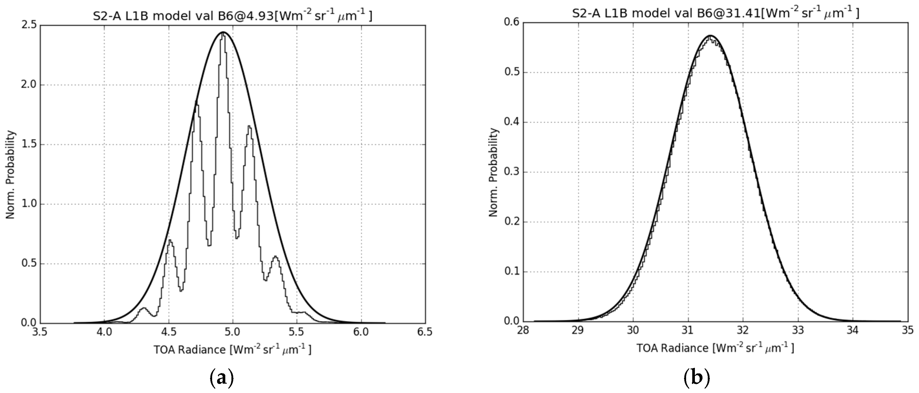
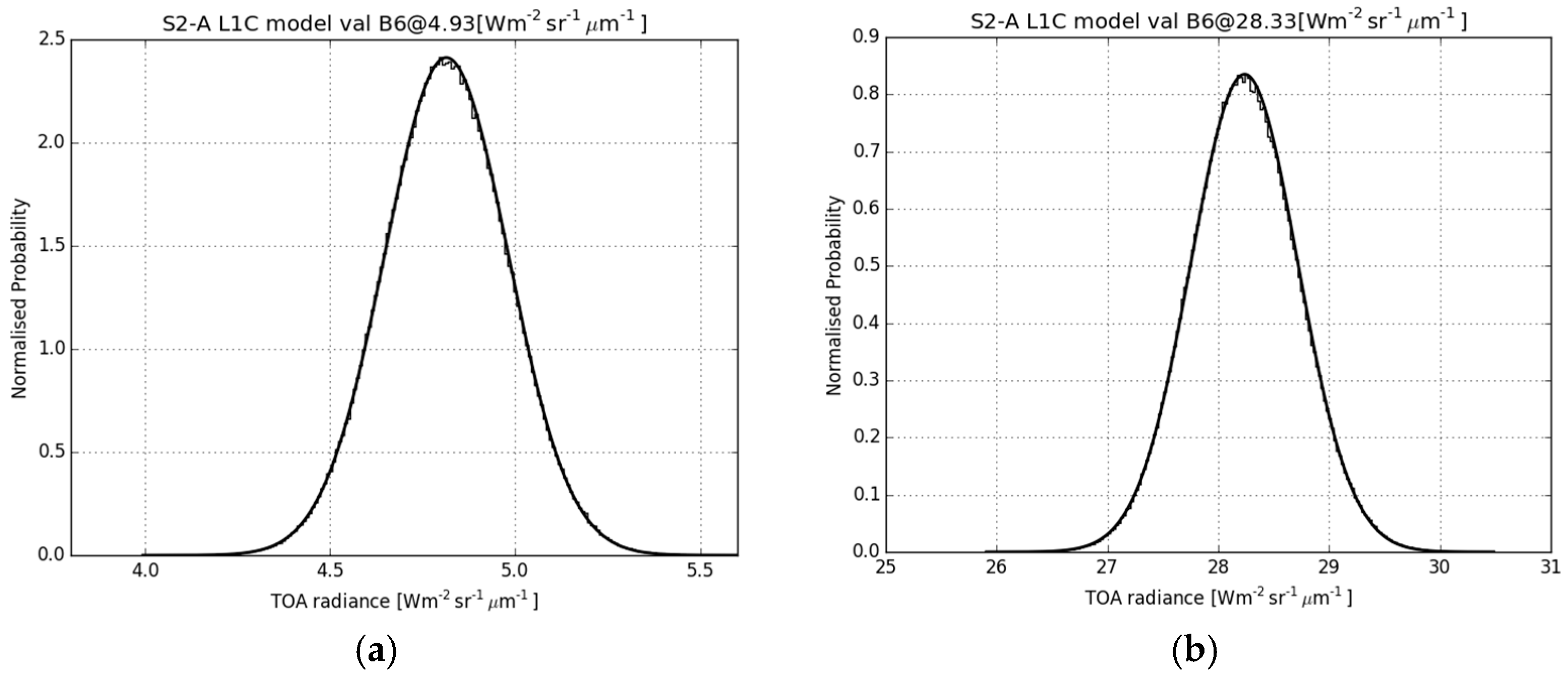
• u_noise vs. u_ADC. The instrument noise is propagated through the ADC quantisation. The two components can be assumed significantly uncorrelated for a noise larger than the quantisation effect. We explore this option further in Section 4.5 since, below a certain limit, the uniform distribution of ADC does not apply and the noise can be modulated by the digital conversion.

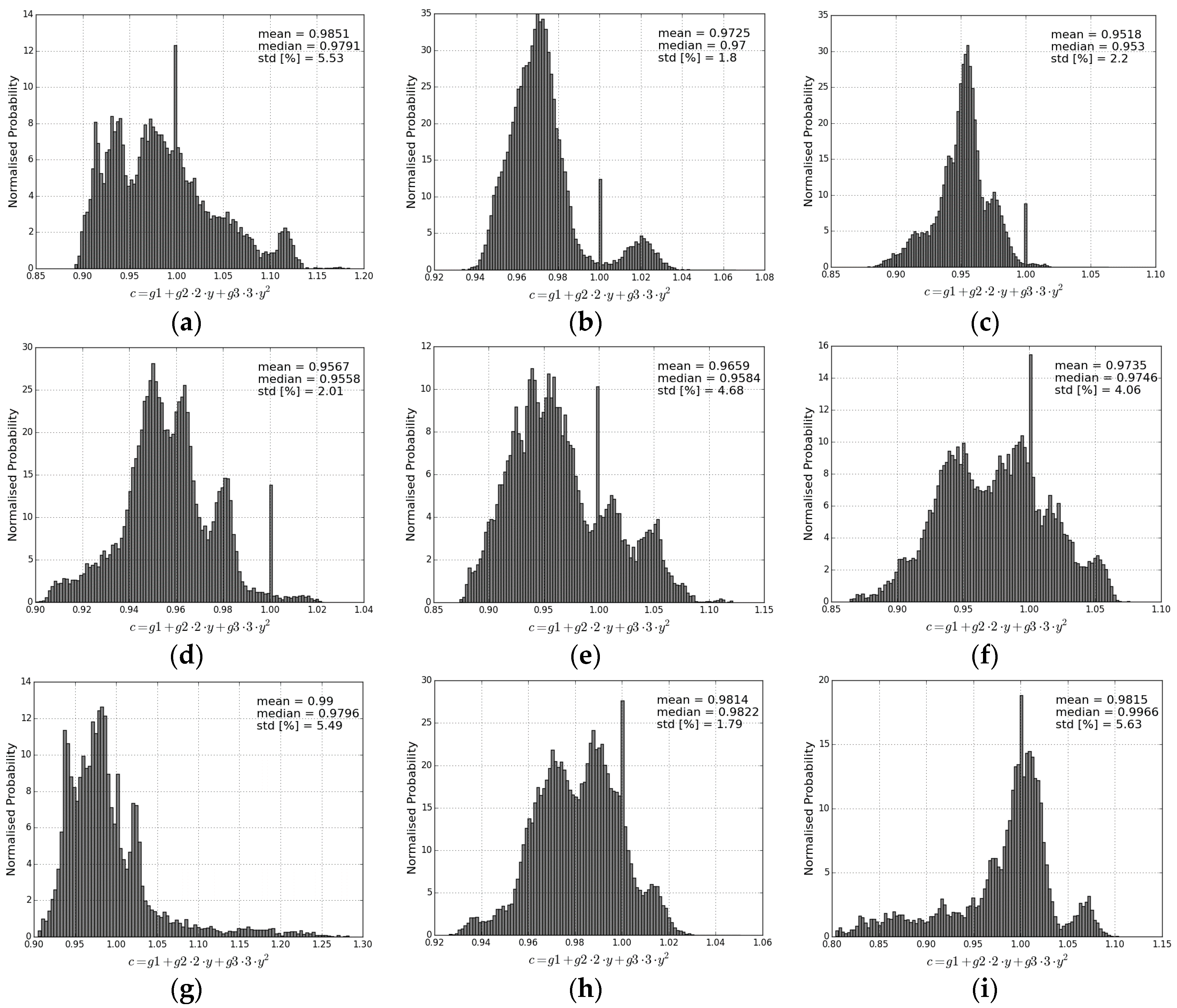
4.5. Validation of the Central Limit Theorem

The combined standard uncertainty in the GUM relies on the propagation of the uncertainty contributions through a linearised measurement model. The associated distribution can be approximated as normal based on the validity assumption of the central limit theorem as described in section G.2 in [8]. Here we provide an initial assessment on how well the GUM method provides a valid uncertainty estimation of the L1 model by comparing the results to a multivariate Monte Carlo Method (MCM), the latter being capable of propagating the uncertainty sources through the full model [29].

In this initial version, several uncertainty contributors concerning the L1 radiometric processing have been considered and listed in

Table 2. Considered uncertainty contributors for the L1B model validation.

L1B Contributor	Value	Distribution Type
Instrument noise, unoise	Calculated as in Equation (9). Coefficients α and β extracted from the datastrip metadata [19]	Normal
ADC quantisation, uADC	±0.5 [LSB]	Rectangular
Dark signal knowledge	±0.05 [LSB]	Normal
Dark signal stability, uDS	±0.1 VNIR, ±0.24 B10, ±0.1 B11, ±0.16LSB B12 [LSB]	Rectangular
Relative gains accuracy	Extracted from quoted L1C metadata (0.4%) [19]	Normal
Diffuser uncertainty	From pre-flight characterisation [25]	Normal
Diffuser angle knowledge	±0.4%	Normal
Kslt residual	±0.3%	Rectangular

. The script automatically reads certain calibration parameters as DS or relative gain coefficients. The version was presented in [16] and expanded to L1C in [17]. The effects of the contributors detailed in Section 3.2.2 and Section 3.2.9 are not considered, since they are added linearly in Equation (13). The contributions of out-of-field stray-light—random part (see Section 3.2.3) and crosstalk (see Section 3.2.4) are also not considered at this stage although it is intended that their distribution and effect should be revisited in later versions and also that these contributions have a low impact on the final results. Table 2 summarises the uncertainty contributions considered, their values and associated distribution:

Figure 4 provides the difference between the GUM uncertainty combination (k = 1) and the area around the mean with approximately 68.27% of output values of the MCM uncertainty distribution. The results are presented for a range between L_min and L_ref approximately.

The results in Figure 4 clearly show the validity of the GUM framework for the L1B product with disagreement <0.1% between both methods (GUM vs. MCM) for the majority of the radiance range. For low radiance values, the use of the GUM approach does not represent a reliable parameter to characterise the uncertainty. At this low level of radiance, the ADC noise becomes unstable and invalidates the central limit theorem.

The majority of land scenes will generally measure radiances where this effect is not applicable or negligible. However, it could be that specific scenes, such as very dark vegetation forest or case-2 water scenes, are near the radiance levels where the GUM approach becomes unreliable.

The bands B3-B8A have the larger dynamic range and, at extremely low light levels, the quantisation becomes dominant. Figure 5 shows an example for B6 at different radiance levels.

These two distributions agree for values close to L_ref almost perfectly, demonstrating that the output distribution is fairly normal. However, we can see clearly the effect of the quantisation effect for low radiance values. The answer given in [30] for a normal noise provides an alternative analytical form to understand this effect.

The validation up to L1C involves the propagation through the bi-spline radiometric interpolation as in [17]. The radiance levels in Figure 5 have been propagated assuming a perfectly flat 4 × 4 kernel grid of constant radiance values. As a first assessment, the L1B contributions assume uncorrelated contributions with the exception of the absolute calibration coefficients which are assumed fully correlated in the kernel. The results at two different radiance levels of B6 are shown in Figure 6.

The results show, for this specific case, the reduction of the non-stability of the ADC due to the averaging of the 16 pixels in the kernel. A full validation up to L1C would involve many non-uniform radiance cases to be studied. One of these examples can be found in [17]. However, this is an area that needs to be expanded with more study cases and a refined spatial and temporal correlation study.

In summary, the effect of non-linear corrections when combining the uncertainty contributions is treated as being negligible in the S2-RUTv1, but the unstable effects due to the ADC quantisation invalidate the central limit theorem assumption when evaluating the uncertainty at low radiance levels.

5. Software Implementation and Integration

5.1. Tool Integration, System Requirements and Performance

The development of the tool code is fully accessible in the software repository in [7]. This code works as a plug-in that is embedded as part of the Sentinels Toolbox. Both SNAP and this plug-in support all major platforms, like Windows, UNIX and Mac OS. In order to support the S2 L1C data products, the S2-Toolbox needs to be installed in addition to the bare SNAP installation. Their last releases are available at [12]. Python, as implementation language, needs to be installed and the version must be 2.7 or later. In addition, this Python installation must have the NumPy library installed.

The requirements on the hardware are very dependent on the processing operation and the source data. For S2-RUT, the requirements are not very demanding and it can run in a minimal configuration. On a computer, with an Intel Core i7 processor and 8 GB of RAM, processing all bands of a S2 L1C product at once will roughly take 11–12 min. Computing a single band varies from 5 s to 110 s depending on its resolution.

The S2-RUT works as a set of routines that interface with SNAP. First, SNAP retrieves information from the s2_rut-info.xml for the creation of the user interface for the operator. When the user is satisfied with the configuration, the operator (implemented in the class S2RutOp) can run the code. As a result, the user gets the uncertainty image for the selected band(s). The class S2RutAlgo is called during the process of the uncertainty image generation as it brings the core of the uncertainty calculation. The main features of the tool software design are:

• SNAP Python libraries (snappy) for product readout.
• General tool design to accommodate other sensors.
• Maximisation of product info extraction (e.g., noise coefficients) makes it robust against re‑processing, contingencies etc.
• Conservation of the geolocation information for collocation between the L1C reflectance factor and uncertainty images.

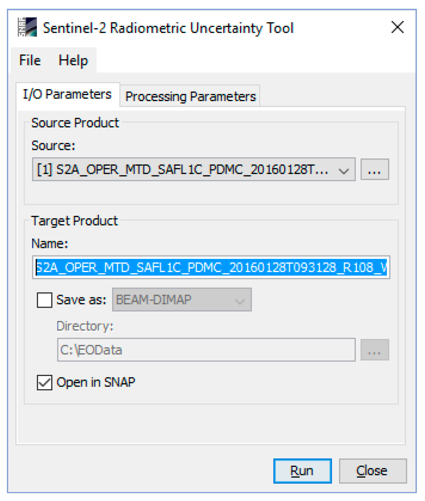
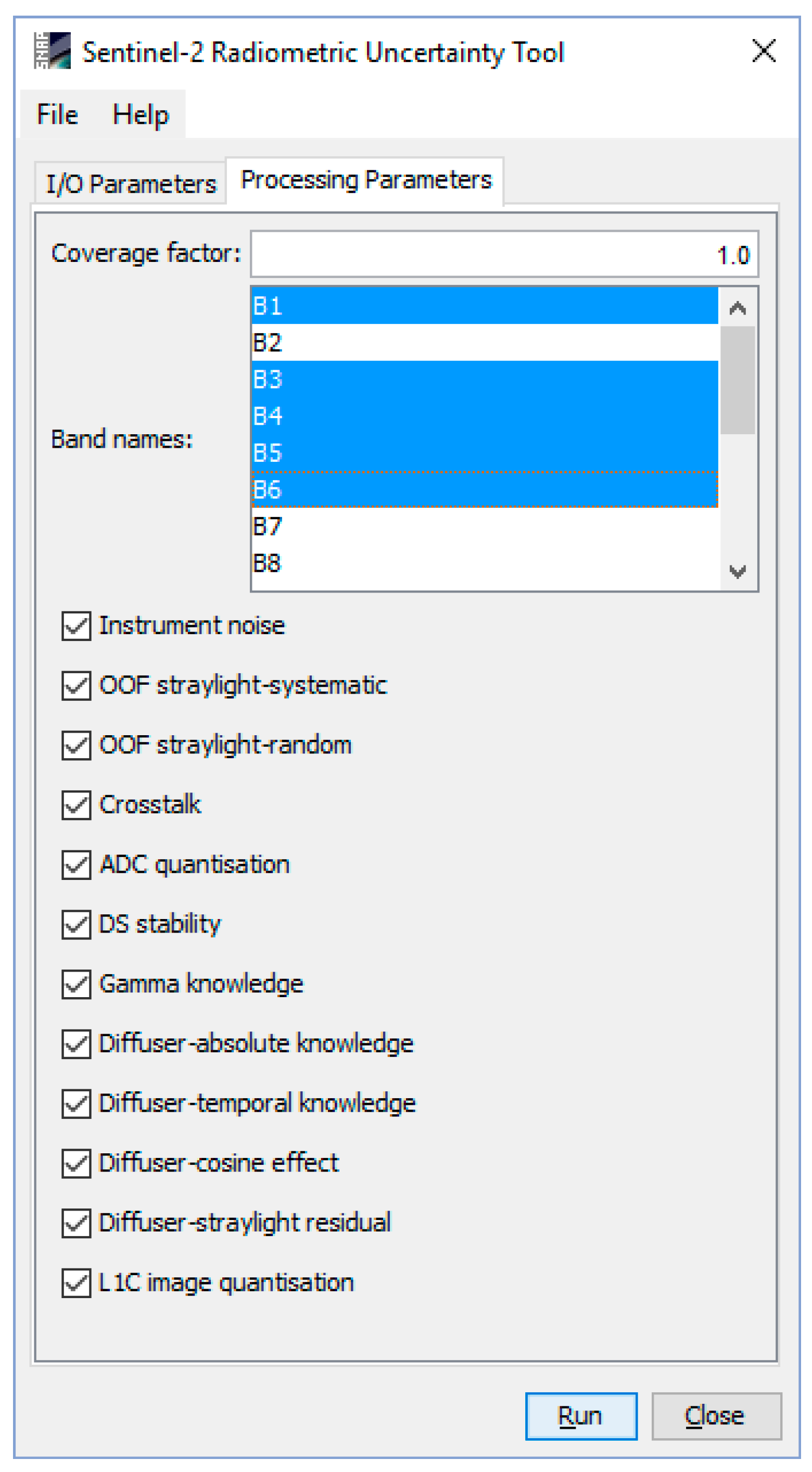
5.2. Processor Documentation

The S2-RUTv1 processor can be invoked in SNAP from the menu by selecting Optical->Preprocessing->Sentinel-2 Radiometric Uncertainty Tool. On the command line processor, available by means of the Graph Processing Tool gpt, which is located in SNAP bin directory, typing gpt S2Rut -h displays further information.

Selecting the Sentinel-2 Radiometric Uncertainty Tool command from the SNAP menu opens up the dialog in Figure 7.

In the “Source product” area, the user specifies the source product. The combo box presents a list of all products opened in SNAP. The user may select one of these or, by clicking on the button next to the combo box, choose a product from the file system. The selected product must be of type S2_MSI_Level-1C. In the “Target product” area, the user can specify a name for the generated product. As a default, the tool will automatically assign a name by adding the extension “_rut” to the Sentinel-2 L1C product selected. The user can also specify where the target product should be saved in the file system. The combo box presents a list of available file formats. The text field or the button next to it allow specification of a target directory. Finally, the option “Open in SNAP” specifies whether the target product should be opened in SNAP. When the target product is not saved, it is opened in the Sentinel Toolbox automatically.

The tool incorporates a secondary tab named “Processing Parameters”. Figure 8 presents a screen-shot as it appears in SNAP.

This tab is intended for expert users and allows different options for the uncertainty combination choices. Standard users have default parameters. Three main sections with multiple options are included in the S2-RUTv1:

• The option “Coverage factor” permits specifying the k parameter that assigns a probability coverage to the uncertainty evaluation—k = 1 means 68.27% probability [8].
• The selection of “Band names” means the uncertainty shall be computed.
• For uncertainty contribution selection, the tab includes a selection list with the uncertainty contributions included in the S2-RUTv1 (see Table 1). This permits the user the selection and deselection of specific contributions in order to perform sensitivity analysis and separation of random/systematic contributions, etc.

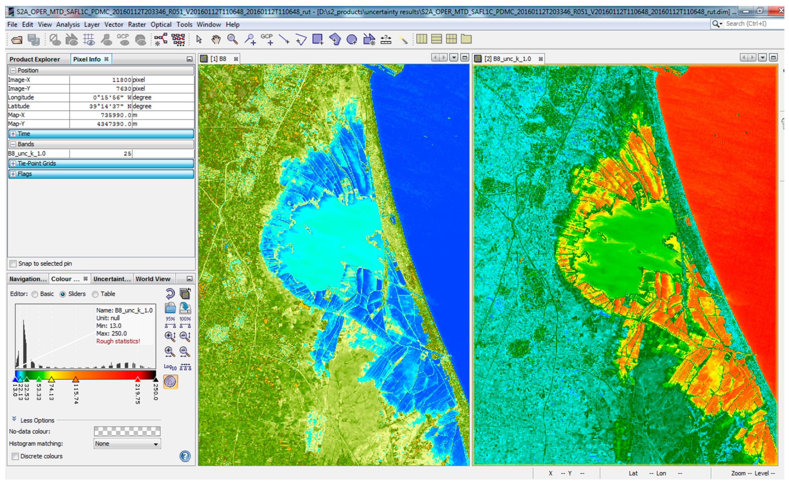
5.3. Output Generation

The uncertainty results at pixel level are codified in UINT8 (i.e., one byte). Values from 0–250 refer to uncertainty values from 0%–25% in steps of 0.1%. The values are clipped to this range so:

• 0 == Invalid uncertainty (it cannot be 0 or negative)
• 250 == Uncertainty ≥25%

This means that the tool can be helpful in managing the GML information in the product masks and include it at a pixel level in the uncertainty image itself in future versions. If the pixel status is “saturated, no data, cloud, and defect,” then the uncertainty evaluation is of course not required and the five values missing—from 251 to 255—could be used to provide raster information of the GML masks.

Another byte image could potentially be included in future versions, and include information regarding specific flags for polarisation or stray-light events as well as information related to the correlation between pixels in the time, space and spectral dimension [16]. To sum up, the idea is that an additional byte becomes a “quality indicator” that supports the calculation of uncertainty and their application.

5.4. Radiometric Uncertainty Tool (RUT) Version 1 (v1) Case Study: Albufera Lake, Spain

Figure 9 shows the result of running the S2-RUTv1 in SNAP for a specific S2 L1C product and band. The area shown represents Albufera Lake in Valencia (Spain) on 12 January 2016 for B8 and its associated uncertainty. The scale of values for both the L1C reflectance factor and uncertainty are shown in Figure 10.

The area surrounding the lake is subject to variations in the water level (rice field) and, depending on the area and overpass time, the variation of uncertainty (in relative units) can change significantly. Figure 9 also indicates how Albufera Lake has lower uncertainty than many of the rice fields due to the large amount of sediments.

The uncertainty—on the right of Figure 9—ranges from >10% for open sea to 5%–6% in the lake body, 5%–15% in the rice fields covered by water and 2%–4% in the land areas. This simple exercise shows how the S2-RUT helps users to assess the level of uncertainty that they can expect for their study area at a particular point in time.

6. Conclusions and Further Work

This paper describes the design and development process of the initial version of the Sentinel 2-Radiometric Uncertainty Tool (S2-RUT) tool. This tool enables users to generate per-pixel radiometric uncertainty associated with the S2 Level 1 (L1C) products. This first version is focused on describing an exhaustive uncertainty methodology and a general software design that can be followed in subsequent versions of the tool and can be readily adapted to several other Earth Observation (EO) missions.

The uncertainty analysis effectively links the uncertainty contributors with the radiometric model. The identified uncertainty contributors are exhaustively assessed and their combination using the ‘Guide to Expression of Uncertainty in Measurement’ (GUM) model is discussed in detail, with a special effort here in validating and discussing the combination model. The uncertainty analysis has flagged and discussed the existence of systematic uncorrected effects in the S2 L1C radiometry.

This initial version of the tool has been implemented—code available at [7]—and integrated as part of Sentinels Application Platform (SNAP). The integration of the S2-RUT tool as part of SNAP facilitates the integration of the uncertainty products in the users’ EO processing and thus does not increase the memory and storage requirements of the operational S2 L1 processing performed at the European Space Agency (ESA). The tool software design looks for an optimal strategy to read the top-of-atmosphere (TOA) reflectance factor images so that they can run on a “standard” computer.

The first version of the tool also includes the assessment of the uncertainty at a desired coverage probability by setting a coverage factor, k, and the selection/deselection of the uncertainty contributors for sensitivity studies.

Although a first version has been fully implemented, there are still several areas to study and incorporate in subsequent versions of the tool. Many of the areas that could be improved in future versions have been mentioned throughout this paper. This would include the introduction of additional uncertainty contributions—note that his work has already started in [17]—and the refinement of some of the uncertainty contributions in S2-RUTv1.

The TOA radiometric uncertainty provided by the S2-RUT is expected to be the input for its propagation through consecutive steps of the EO processing chain similarly to [2]. These higher-level uncertainty estimates will require the covariance information in the spatial, temporal and spectral dimensions. The preliminary results in [17] and in Figure 6 have shown how important the correlation between the different pixels and the need to include this information for combination or propagation of uncertainty estimates are. The implementation of the S2-RUT as an external tool might introduce limitations, and hybrid or full implementation of the covariance might need to be included in the L1 processing as described, for example, in the Kepler mission [31]. Nonetheless, several trade-off analyses and alternatives will need to be considered for its implementation.

The software implementation in future versions would seek to include the new uncertainty contributions and update the results of a refined uncertainty analysis. In addition, it should include the processing of the quality masks’ information of the S2 L1C products as part of the uncertainty image itself (see Section 5.3). Use of quality flags related to polarisation and stray-light effects as specified in Section 5.3 or covariance information may be included as a second byte codification. The interface with other SNAP plug‑ins might enhance even further the possibilities of the tool.

References

1. QA4EO. A Quality Assurance Framework for Earth Observation: Principles. Available online: http://qa4eo.org/docs/QA4EO_Principles_v4.0.pdf (accessed on 24 January 2017).
2. Merchant, C.J.; Embury, O.; Roberts-Jones, J.; Fiedler, E.; Bulgin, C.E.; Corlett, G.K.; Good, S.; McLaren, A.; Rayner, N.; Morak-Bozzo, S.; et al. Sea surface temperature datasets for climate applications from phase 1 of the European Space Agency climate change initiative (SST CCI). Geosci. Data J. 2014, 1, 179–191. [Google Scholar] [CrossRef]
3. Gardner, J.L. Uncertainty propagation for NIST visible spectral standards. J. Res. Natl. Inst. Stand. Technol. 2004, 109, 305–318. [Google Scholar] [CrossRef] [PubMed]
4. Esposito, J.A.; Xiong, X.; Wu, A.; Sun, J.; Barnes, W.L. MODIS reflective solar bands uncertainty analysis. Proc. SPIE 2004. [Google Scholar] [CrossRef]
5. Xiong, X.; Troller, G.; Sun, J.; Wenny, B.; Angal, A.; Barnes, W. MODIS Level 1b Algorithm Theoretical Basis Document; NASA/Goddard Space Flight Center: Greenbelt, MD, USA, 2013.
6. Toller, G.N.; Isaacman, A.; Kuyper, J. Modis Level 1b Product User’s Guide; NASA/Goddard Space Flight Center: Greenbelt, MD, USA, 2006.
7. Gorroño, J.; Fomferra, N.; Peters, M. Sentinel-2 Radiometric Uncertainty Tool (S2-RUT). Available online: https://github.com/senbox-org/snap-rut (accessed on 24 January 2017).
8. JCGM. Guide to the Expression of Uncertainty in Measurement. Available online: http://www.bipm.org/en/publications/guides/gum.html (accessed on 24 January 2017).
9. Lefebvre, A.; Sannier, C.; Corpetti, T. Monitoring urban areas with Sentinel-2a data: Application to the update of the copernicus high resolution layer imperviousness degree. Remote Sens. 2016, 8, 606. [Google Scholar] [CrossRef]
10. Immitzer, M.; Vuolo, F.; Atzberger, C. First experience with Sentinel-2 data for crop and tree species classifications in central europe. Remote Sens. 2016, 8, 166. [Google Scholar] [CrossRef]
11. Drusch, M.; Del Bello, U.; Carlier, S.; Colin, O.; Fernandez, V.; Gascon, F.; Hoersch, B.; Isola, C.; Laberinti, P.; Martimort, P.; et al. Sentinel-2: ESA’S optical high-resolution mission for gmes operational services. Remote Sens. Environ. 2012, 120, 25–36. [Google Scholar] [CrossRef]
12. ESA (European Space Agency). Snap and the Sentinel Toolboxes. Available online: http://step.esa.int/main/download/ (accessed on 24 January 2017).
13. Gascon, F.; Cadau, E.; Colin, O.; Hoersch, B.; Isola, C.; López Fernández, B.; Martimort, P. Copernicus Sentinel-2 mission: Products, algorithms and Cal/Val. Proc. SPIE 2014. [Google Scholar] [CrossRef]
14. ESA (European Space Agency). Sentinel-2 MSI Technical Guide. Available online: https://sentinel.esa.int/web/sentinel/technical-guides/sentinel-2-msi (accessed on 24 January 2017).
15. Thuillier, G.; Hersé, M.; Labs, D.; Foujols, T.; Peetermans, W.; Gillotay, D.; Simon, P.C.; Mandel, H. The solar spectral irradiance from 200 to 2400 nm as measured by the solspec spectrometer from the atlas and EURECA missions. Sol. Phys. 2003, 214, 1–22. [Google Scholar] [CrossRef]
16. Gorroño, J.; Gascon, F.; Fox, N.P. Radiometric uncertainty per pixel for the Sentinel-2 L1C products. Proc. SPIE 2015. [Google Scholar] [CrossRef]
17. Gorroño, J.; Banks, A.; Gascon, F.; Fox, N.P.; Underwood, C.I. Novel techniques for the analysis of the TOA radiometric uncertainty. Proc. SPIE 2016. [Google Scholar] [CrossRef]
18. Barsi, J.; Lee, K.; Kvaran, G.; Markham, B.; Pedelty, J. The spectral response of the Landsat-8 operational land imager. Remote Sens. 2014, 6, 10232. [Google Scholar] [CrossRef]
19. Gatti, A.; Bertolini, A. Sentinel-2 Products Specification Document v.14.2. Available online: https://sentinel.esa.int/web/sentinel/document-library/content/-/article/sentinel-2-level-1-to-level-1c-product-specifications (accessed on 24 January 2017).
20. Janesick, J.; Pinter, J.; Potter, R.; Elliott, T.; Andrews, J.; Tower, J.; Grygon, M.; Keller, D. Fundamental performance differences between CMOS and CCD imagers, Part IV. Proc. SPIE 2010. [Google Scholar] [CrossRef]
21. Arrhenius, S.; Pamphlets, P. Über Die Dissociationswärme und den Einfluss der Temperatur auf den Dissociationsgrad der Elektrolyte; Wilhelm Engelmann: Berlin, Germany, 1889. [Google Scholar]
22. Hopkinson, G.R.; Goodman, T.M.; Prince, S.R. A Guide to the Use and Calibration of Detector Array Equipment; SPIE Press: Orlando, FL, USA, 2004. [Google Scholar]
23. Dariel, A.; Chorier, P.; Leroy, C.; Maltère, A.; Bourrillon, V.; Terrier, B.; Molina, M.; Martino, F. Development of an SWIR multispectral detector for GMES/Sentinel-2. Proc. SPIE 2009. [Google Scholar] [CrossRef]
24. Espuche, S.; Chorvalli, V.; Laborie, A.; Delbru, F.; Thomas, S.; Sagne, J.; Haas, C. VNIR focal plane results from the multispectral instrument of the Sentinel2 mission. In Proceedings of the ICSO 2014 International Conference on Space Optics, Tenerife, Spain, 6–10 October 2014.
25. Mazy, E.; Camus, F.; Chorvalli, V.; Domken, I.; Laborie, A.; Marcotte, S.; Stockman, Y. Sentinel-2 diffuser on-ground calibration. Proc. SPIE 2013. [Google Scholar] [CrossRef]
26. Rahman, H.; Pinty, B.; Verstraete, M.M. Coupled Surface-Atmosphere Reflectance (CSAR) Model: 2. Semiempirical surface model usable with NOAA advanced very high resolution radiometer data. J. Geophys. Res. Atmos. 1993, 98, 20791–20801. [Google Scholar] [CrossRef]
27. Stiegman, A.E.; Bruegge, C.J.; Springsteen, A.W. Ultraviolet stability and contamination analysis of spectralon diffuse reflectance material. Opt. Eng. 1993, 32, 799–804. [Google Scholar] [CrossRef]
28. Delwart, S.; Bourg, L. Radiometric calibration of MERIS. Proc. SPIE 2011. [Google Scholar] [CrossRef]
29. JCGM. Evaluation of Measurement Data—Supplement 1 to the “Guide to the Expression of Uncertainty in Measurement”—Propagation of Distributions Using a Monte Carlo Method. Available online: http://www.bipm.org/en/publications/guides/gum.html (accessed on 24 January 2017).
30. Carbone, P.; Petri, D. Mean value and variance of noisy quantized data. Measurement 1998, 23, 131–144. [Google Scholar] [CrossRef]
31. Clarke, B.D.; Allen, C.; Bryson, S.T.; Caldwell, D.A.; Chandrasekaran, H.; Cote, M.T.; Girouard, F.; Jenkins, J.M.; Klaus, T.C.; Li, J.; et al. A framework for propagation of uncertainties in the Kepler data analysis pipeline. Proc. SPIE 2010. [Google Scholar] [CrossRef]
Figure 1. Illustration of the MultiSpectral Instrument (MSI) radiometric model and Level 1 (L1) ground processing with the associated parameters described in Equations (1)–(8).
Remotesensing 09 00178 g001
Figure 2. Distribution of the sensitivity coefficient cy for all the pixels in the Sentinel-2 (S2) Visible and Near-InfraRed (VNIR) bands (a) B1; (b) B2; (c) B3; (d) B4; (e) B5; (f) B6; (g) B7; (h) B8 and (i) B8A.
Remotesensing 09 00178 g002
Figure 3. Distribution of the sensitivity coefficient cy for all the pixels in the S2 Short-Wave InfraRed (SWIR) bands parameter a1 (a) B11; (b) B12 and parameter a2; (c) B11; (d) B12.
Remotesensing 09 00178 g003
Figure 4. S2 L1B model validation for the S2 bands (a) B1; (b) B2; (c) B3; (d) B4; (e) B5; (f) B6; (g) B7; (h) B8; (i) B8A; (j) B11; and (k) B12. The graph compares the ‘Guide to Expression of Uncertainty in Measurement’ (GUM) uncertainty (k = 1) to the 68.27% area of the Monte Carlo Method (MCM) symmetric from its mean.
Remotesensing 09 00178 g004
Figure 5. L1B MCM distribution at (a) 4.93 Wm−2·sr−1·μm−1 and (b) 31.41 Wm−2·sr−1·μm−1. The theoretical normal distribution of the combined standard uncertainty has been included and re-scaled to the MCM distribution peak value for comparison.
Remotesensing 09 00178 g005
Figure 6. L1C MCM distribution at (a) 4.93 Wm−2·sr−1·μm−1 and (b) 28.33 Wm−2·sr−1·μm−1. The theoretical normal distribution of the combined standard uncertainty has been included and re-scaled to the MCM distribution peak value for comparison. The resampling introduces a fully correlated absolute calibration coefficient uncertainty A(b) for the L1B measurements using bi-splines.
Remotesensing 09 00178 g006
Figure 7. Screen-shot of the “I/O Parameters” tab of Radiometric Uncertainty Tool (RUT) tool as integrated in Sentinel Application Platform (SNAP).
Remotesensing 09 00178 g007
Figure 8. Screen-shot of the “Processing Parameters” tab of RUT tool as integrated in SNAP.
Remotesensing 09 00178 g008
Figure 9. Screen-shot of SNAP. It contains the pixel info and navigation panels (left); the L1C Sentinel-2 B8 image for Albufera Lake (centre) and the equivalent uncertainty k=1 (right). The image is North oriented.
Remotesensing 09 00178 g009
Figure 10. Screen-shot of L1C reflectance factor scale in Figure 9 (up); and the scale of equivalent uncertainty k = 1 (down). The L1C reflectance factor is multiplied by the quantification value of 10,000 and the uncertainty figures are given as percentages multiplied by 10.
Remotesensing 09 00178 g010