Article

Assessing the Potential of Sentinel-2 and Pléiades Data for the Detection of Prosopis and Vachellia spp. in Kenya

1
Institute for Surveying, Remote Sensing and Land Information, University of Natural Resources and Life Sciences, Vienna (BOKU), Peter Jordan Str. 82, A-1190 Vienna, Austria
2
Kenya Forestry Research Institute (KEFRI), Baringo Sub Centre, P.O. BOX 57-30403, Marigat, Kenya
3
Faculty of Arts and Humanities, Department of Geography, Chuka University, P.O. Box 109-60400, Chuka, Kenya
4
Centre for Development and Environment, University of Bern, Hallerstrasse 10, CH-3012 Bern, Switzerland
*
Author to whom correspondence should be addressed.
Remote Sens. 2017, 9(1), 74; https://doi.org/10.3390/rs9010074
Submission received: 9 September 2016 / Revised: 20 December 2016 / Accepted: 2 January 2017 / Published: 16 January 2017

Abstract

:
Prosopis was introduced to Baringo, Kenya in the early 1980s for provision of fuelwood and for controlling desertification through the Fuelwood Afforestation Extension Project (FAEP). Since then, Prosopis has hybridized and spread throughout the region. Prosopis has negative ecological impacts on biodiversity and socio-economic effects on livelihoods. Vachellia tortilis, on the other hand, is the dominant indigenous tree species in Baringo and is an important natural resource, mostly preferred for wood, fodder and charcoal production. High utilization due to anthropogenic pressure is affecting the Vachellia populations, whereas the well adapted Prosopis—competing for nutrients and water—has the potential to replace the native Vachellia vegetation. It is vital that both species are mapped in detail to inform stakeholders and for designing management strategies for controlling the Prosopis invasion. For the Baringo area, few remote sensing studies have been carried out. We propose a detailed and robust object-based Random Forest (RF) classification on high spatial resolution Sentinel-2 (ten meter) and Pléiades (two meter) data to detect Prosopis and Vachellia spp. for Marigat sub-county, Baringo, Kenya. In situ reference data were collected to train a RF classifier. Classification results were validated by comparing the outputs to independent reference data of test sites from the “Woody Weeds” project and the Out-Of-Bag (OOB) confusion matrix generated in RF. Our results indicate that both datasets are suitable for object-based Prosopis and Vachellia classification. Higher accuracies were obtained by using the higher spatial resolution Pléiades data (OOB accuracy 0.83 and independent reference accuracy 0.87–0.91) compared to the Sentinel-2 data (OOB accuracy 0.79 and independent reference accuracy 0.80–0.96). We conclude that it is possible to separate Prosopis and Vachellia with good accuracy using the Random Forest classifier. Given the cost of Pléiades, the free of charge Sentinel-2 data provide a viable alternative as the increased spectral resolution compensates for the lack of spatial resolution. With global revisit times of five days from next year onwards, Sentinel-2 based classifications can probably be further improved by using temporal information in addition to the spectral signatures.

Graphical Abstract

1. Introduction

Invasive species cause ecological, economic and social impacts and are key drivers of global change [1]. Prosopis spp., mesquite, which are native to arid and semi-arid zones in the Americas, are among the world’s most damaging invasive species. Globally, they are regarded as noxious invaders having substantial impacts on biodiversity, ecosystem services, as well as on local and regional economies in their native and even more so in their invasive ranges [2]. According to Shackleton et al. [2] factors that make many Prosopis species successful invaders are: (a) the production of a large number of seeds that remain viable for decades; (b) rapid growth rates; (c) the ability to coppice after damage [3,4,5]; (d) a root system that taps deep into the groundwater table [6,7]; (e) a high tolerance to climate extremes; (f) a high tolerance to various soil types; and (g) negative allelopathic effects on competing plants [8].
Prosopis spp. were introduced to Kenya by the Food and Agriculture Organization (FAO) in the early 1980s [9,10]. The aims were to prevent desertification, provide an alternative fuelwood to the high demand for Vachellia, and reduce stress on indigenous flora by the human population [1,9]. According to Andersson [10], a large number of Prosopis plantations were created around Lake Baringo propagating Prosopis juliflora (Sw.) DC. and/or the closely related Prosopis pallida (Willd.) Kunth (16 sites) as well as Prosopis chilensis (Molina) Stuntz (17 sites). Additionally, small scale plantations were established for the creation of ornamental plants. A summary of Prosopis plantations in Kenya, derived from the work of Andersson, is provided in Table 1 [10].
Over time, these species and their hybrid offspring, described by Pasiecznik et al. [11] as the Prosopis julifloraProsopis pallida complex, earned themselves a spot on the World Conservation Unions 100 of the “world’s worst invasive alien species” list [12]. In our study, we address all Prosopis ssp. and hybrids as Prosopis.
The genus Acacia sensu lato is a large genus consisting of over 900 different species. Since 2005, the African species are recognized as Vachellia [13], as previously the nomenclature identified the African varieties as Acacia spp. Vachellia tortilis (Forssk.) Hayne Galasso and Banfi is among the six endemic Vachellia species present in Baringo [14] and the most dominant prolific species in the study area. The deciduous tree species is utilized for numerous livelihood activities in semi-arid parts throughout Kenya [14], such as: (a) production of charcoal; (b) supply of timber wood; (c) provision of fodder for livestock [9]; and (d) production of honey [14]. Its intensive use causes substantial disturbance on the species and decreases its competitiveness, which makes vast areas susceptible to Prosopis [15]. In this paper, we refer to and simplify all Vachellia subspecies, including the nomenclature re-classification, present at our study site as Vachellia.
Prosopis and Vachellia species have in principle similar characteristics (Figure 1), in that both are drought tolerant with extensive rooting systems. When comparing the roots, Prosopis rapidly develops a complex and vigorous rooting system as a coping mechanism to survive the first dry season [16]. Compared to Vachellia, the species has an extended root depth, reaching deeper aquifers [17]. Both species produce palatable pods [10] which are eaten by many domesticated and wild animals. This enhances seed germination after passing through the digestive system [3] and further propagates the species [18]. A fully developed Prosopis tree yields between 10 and 50 kg of pods annually [19], with approximately 20 to 35 thousand seeds per kg [20]. For comparison, mature Vachellia yields roughly 10 to 12 kg of pods annually containing 12 to 25 thousand seeds per kg [21]. Furthermore, Vachellia trees are subjected to extensive browsing pressure by goats, which stunts young trees in their development [14], while the leaves of Prosopis are non-palatable. Finally, the value of Vachellia charcoal outmatches the value of Prosopis charcoal. All these factors create favorable conditions for Prosopis proliferation.
Remote sensing provides cost-efficient means to assess the distribution of invasive alien plant species and monitor their spread [24,25]. Moreover, it allows assessing areas that are difficult to access. In the past, various attempts have been made to map Prosopis using remote sensing approaches [26,27,28]. Based on the increasing problems caused by Prosopis invasion as well as reported observation that the plant has a distinct spectral response compared to surrounding native vegetation, several mappings have been carried out. In Ethiopia, Wakie et al. [29] have used Moderate Resolution Imaging Spectroradiometer (MODIS) vegetation indices and topo-climatic predictors to map the current distribution of Prosopis using maximum entropy modeling software (Maxent). The performances of the models were evaluated using area under the receiver-operating characteristic (ROC) curve (AUC). The results indicate that the extent the invasion is approximately 3605 km2 in the Afar region (AUC = 0.94), while the potential habitat for future infestations is 5024 km2 (AUC = 0.95). Ayanu et al. [30] applied a combination of Landsat and ASTER data and a supervised classification approach (maximum likelihood) to assess the spreading of Prosopis over the last 30 years. In South Africa, Van den Berg et al. [31] used a combination of Landsat satellite and topographic data and developed a decision tree and threshold based approach to map Prosopis. Both methods focused solely on Prosopis vegetation. Their approaches are based on the assumption that during dry season Prosopis is the most photosynthetically active plant species compared to the other vegetation types present in their respective study area. Supervised classifications with the aim of differentiating Prosopis from other classes were conducted by Robinson et al. [32] classifying Prosopis, Eucalyptus and different soil types in Australia using WorldView-2 very high resolution (VHR) satellite data. In Somaliland, Meroni et al. [27] attempted to differentiate several Prosopis sub-classes, native vegetation as well as mixed vegetation classes based on Landsat 8 satellite data applying a Random Forest (RF) classifier. Ng et al. [28] assessed both object- and pixel-based approaches for detecting Prosopis in Somaliland using Landsat 8 data. Their results show higher accuracies using a pixel-based RF classifier as Landsat’s spatial resolution and extent of the invasion provided higher inaccuracy using an object-based approach. Besides that, there are a modest number of published works describing moderate success using maximum likelihood classifiers and Landsat data for Prosopis detection within Kenya [33,34].
With respect to Baringo County, few attempts have been made to map Prosopis invasion with remote sensing data [35]. Amboka and Ngigi [35] used Landsat time series to detect Prosopis cover in Baringo between 1985 and 2010 using five-year intervals. Their study applied a maximum likelihood classification and was validated through 250 randomly generated and interpreted reference points. The studies outcomes indicate an irregular distribution over time, with a Prosopis cover of 56% of the total land cover in 2005 and an overall accuracy of 89.5%. These results should be scrutinized carefully and indicate that an improved remote sensing study is warranted. Andersson [10] attempted to monitor Prosopis invasion in Baringo by mapping the initial plantations and quantifying the abundance of indigenous plant species in and around these sites. These two studies utilized local knowledge of the study area and plantation sites, without focusing on remote sensing techniques; plant inventories were made along transects. Other research in Bargino focused on impacts of Prosopis invasion on livelihoods [17], costs of controlling the invasion and local residents’ perceptions on Prosopis invasion [36], management, control and utilization of Prosopis [19,20]. However, detailed mapping of Prosopis using higher spatial resolution data and better performing classifiers has not been achieved for Baringo.
Regarding such VHR datasets, imagery under five meter ground sampling distance are labeled as high resolution while imagery under two meter are described as very high resolution [37], two trends can be observed. First, the number of available commercial very high resolution sensors increases steadily, thereby increasing data availability and affordability. Second, Europe’s ambitious Currently, Copernicus program provides free-of-charge Sentinel-2 imagery at high spatial resolution (ten meter). Compared to Landsat satellites, the increased spatial resolution of Sentinel-2, as well as commercial VHR satellites, is expected to provide more accurate results [26] and offering the capacity to distinguish between different species in mixed stands. The discrimination between different species in mixed stands is an essential component of the detection of the Prosopis invasion and classification between Vachellia and Prosopis.
Whereas a large number of studies have been published using VHR satellites for vegetation applications, this is not yet the case for Sentinel-2. Due to the sensor’s novelty (the first of two identical satellites was launched in June 2015), the full range of its capacities has not yet been fully explored. There are only a limited number of published studies dealing with Object-Based Image Analysis (OBIA) and remote sensing of vegetation using this sensor [38,39]. First impressions with focus on vegetation are described by Immitzer et al. [40] and Radoux et al. [41]. Both studies report good classification results regarding the detection of different tree species, crop types and sub-pixel landscape features such as grass strips and small woody patches within European and US test sites. No study is known employing Sentinel-2 for the mapping of invasive species.
Our research aims at addressing several knowledge gaps and needs:
(a)
identify a robust and reliable method for differentiating Prosopis from native vegetation types (Vachellia spp.), including mixed classes;
(b)
produce reliable mapping products having good accuracies, validated with independent reference samples;
(c)
assess the novel Sentinel-2 sensor for tree species classification and its application in arid and semi-arid environments; and
(d)
assess the value of free-of-charge Sentinel-2 data, compared to commercial Pléiades data.

2. Materials and Methods

Maps were created using two different, rather novel, high resolution satellite sensor datasets: Sentinel-2 and Pléiades. The mapping was done using an object-based classification approach and the random forest (RF) classifier. Object-based approaches have distinct advantages when (very) high resolution optical satellite data are used.

2.1. Study Area

The study area is located in the lowlands flats around Lake Baringo, between latitudes 00°21’N and 00°36’N and longitudes 35°55′E and 36°05′E (Figure 2). Marigat is the largest town within the region of interest (ROI), located southwest of Lake Baringo and alongside the Perkerra irrigation scheme. The semi-arid [42] study area is characterized by a unique combination of altitude, precipitation, soil and vegetation. The lowland flats are slightly undulating, dominated by rangeland, with an average altitude of 900 m above sea level (a.s.l.) and surrounded by Tugen hills, ridges and plateaus of the Lake Baringo catchment with peaks of over 2300 m a.s.l. [43]. The total annual rainfall range is 300–700 mm, characterized by bimodal distribution with two peaks in April and November [44].
Presently, the vegetation is bushy, dominated by Prosopis and scattered indigenous species (shrubs and trees) of Vachellia spp., Acalypha fruticosa and Balanites aegyptiaca among others. The soils are moderately to poorly drained, very deep, strongly calcareous, saline and sodic in some areas [3]. The texture is fine sandy loam to clay. The population density is 50 persons per km2 according to 2009 census [45]. The economic activities include livestock, bee keeping, farming and fishing in Lake Baringo. Most lands are held under the communal tenure regime, where land is managed through a common property arrangement [36]. Under this regime, the animals, primarily cows, goats and sheep, are able to move and graze freely. The latter point is important, as a number of studies have indicated that livestock play a major role in contributing to the spread of Prosopis [3,18].

2.2. Data

2.2.1. Satellite Data

For this research, we tested satellite datasets of two different sensors, Sentinel-2 and Pléiades. Sentinel-2 provides free of charge high spatial resolution data at ten meter, whereas Pléiades is a commercial sensor that captures data at very high spatial resolution at two meter (Table 2). Although the acquisition dates of the two images are one year apart, we believe that the two datasets can be well compared as they were acquired within one week of the same season. As a result, climatic and phenological conditions are probably very similar. The scenes have been selected, because both are free of cloud cover.
Pléiades-1A is a commercial sensor operated since December 2011 by Centre National d’Etudes Spatiales (CNES) with a very high spatial resolution of 2 m for four multi-spectral (MS) bands (red, green, blue and near infrared) and one panchromatic (PAN) band at 0.5 m (Figure 3). The sun-synchronous sensor has a revisit time of 26 days and has exceptional roll, pitch and yaw agility, enabling the system to maximize the number of acquisitions above a given area. For analysis, the four multi-spectral bands at original 2 m spatial resolution were used.
Sentinel-2 is a state of the art sensor launched on 23 June 2015 by the European Space Agency (ESA). Sentinel-2 mission is a land monitoring constellation of two identical satellites (Sentinel-2A and Sentinel-2B) that deliver high resolution optical imagery. The system provides a global coverage of the Earth’s land surface and is characterized by its high revisit time (ten days with one satellite and 5 days when Sentinel-2B becomes operational; its launch is scheduled for 2017). The system is designed to collect data at 10 m (blue, green, red and near-infrared-1) and respectively, 20 m (red edge 1 to 3, near-infrared-2, short wave infrared 1 and 2). Three additional bands for atmospheric correction are collected at 60 m (for retrieval of aerosol, water vapor, cirrus), resulting in a total of 13 spectral bands (Figure 3). For our study we excluded the bands having 60 m resolution and resampled all bands to 10 m spatial resolution, effectively down-scaling one 20 m × 20 m pixel into four 10 m × 10 m pixels.
The Sentinel-2 data were corrected for atmospheric effects by applying the Sen2Cor version 2.2.1 software [47]. The atmospheric correction transforms the Top-Of Atmosphere level 1C product to Bottom-Of Atmosphere atmospheric and terrain corrected product (level 2A) and its usability are described by Vuolo et al. [48]. The Pléiades data were atmospherically corrected to a Top-Of-Canopy reflectance dataset using the optical calibration tool implemented in Orfeo toolbox (OTB) [49] which acquires the spectral sensitivity data from the metadata for calibration.

2.2.2. Reference Data
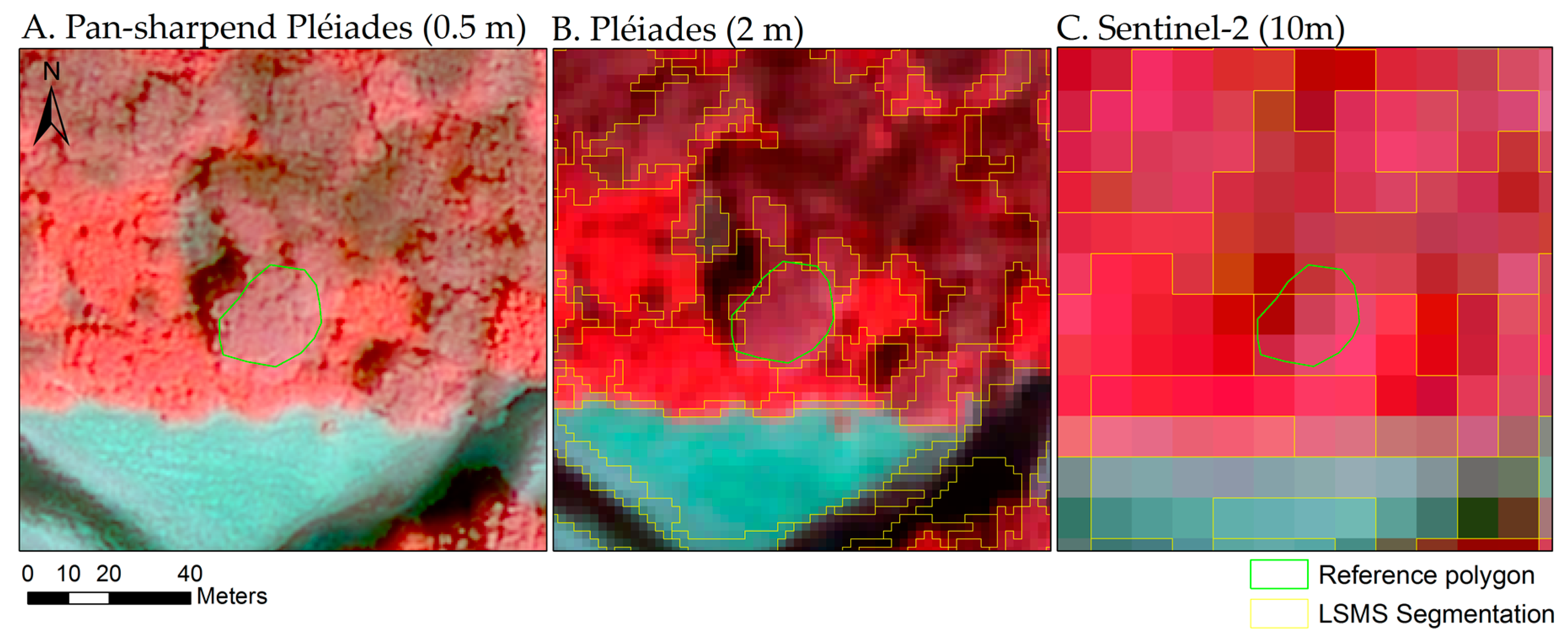
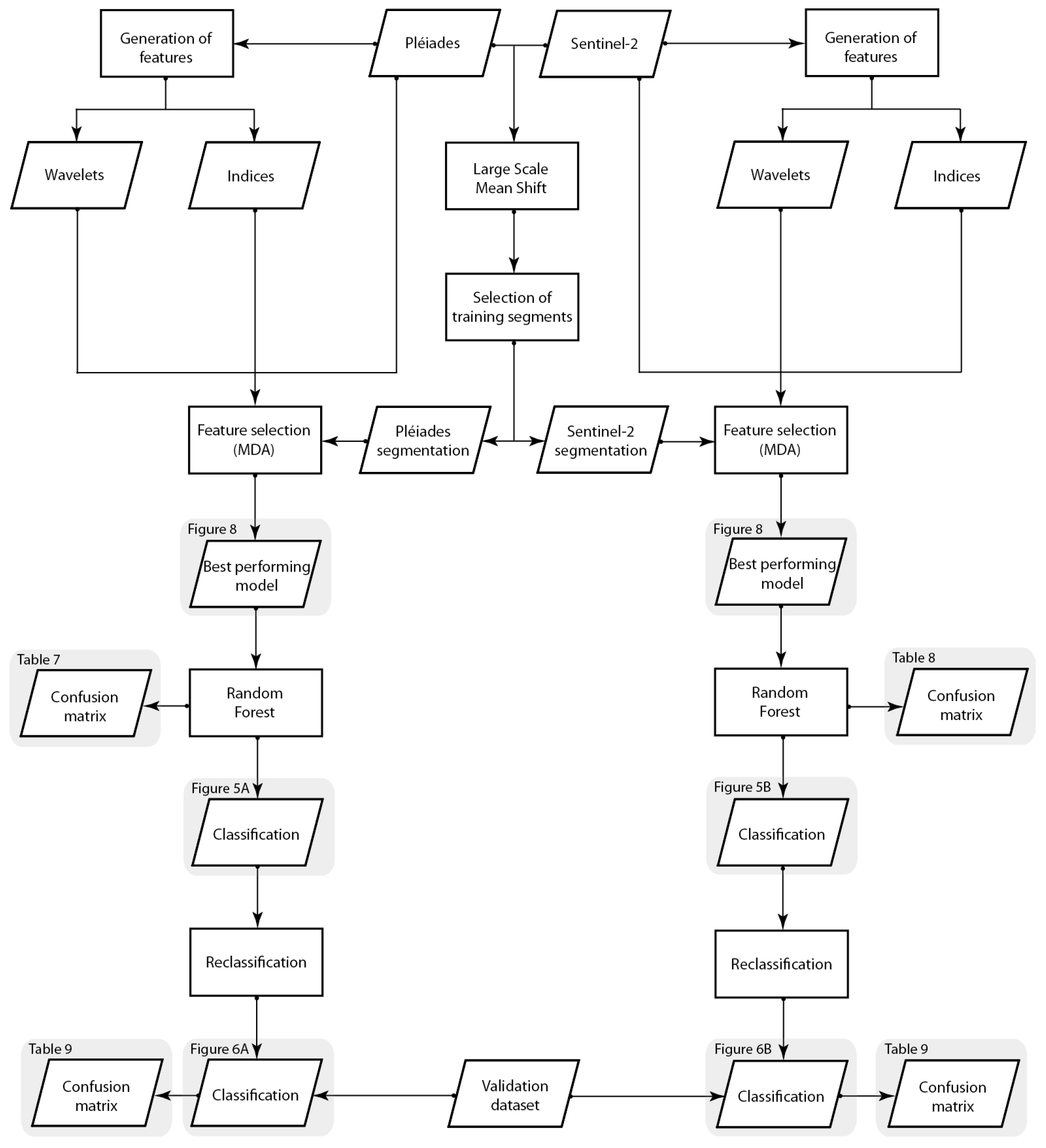
We applied two reference dataset in our study; one for training and another for validation. Field observations for the training data (Figure 2) were collected in May 2016 with a handheld Trimble Juno 3, achieving accuracies between three to five meter. Consisting of approximately 100 GPS-based geo-referenced field data points for Prosopis (n = 43), Vachellia spp. (n = 24) and the mixed classes (n = 31), distributed equally over the study area. For each field data point, we registered species composition (focusing on Prosopis and Vachellia), radius of the plot (10–60 m), fractional vegetation cover, soil type as well as elevation. All field data points were complemented with ample field photographs, taken from the target as well as cardinal directions. Later on, we used the field photographs and Google Earth imagery [50] to complete the training dataset for not surveyed classes such as water and soils. The classification scheme employed for this study is shown in Table 3. Besides a “full” classification with 12 different classes, we also re-classified (regrouped) the original classes into four broad classes (Table 3).
Regarding the second (validation) dataset, approximately 200 GPS points were collected from a parallel study using a handheld Garmin GPS. This dataset is completely independent from the training dataset and is not used for RF training. The independent reference samples were acquired as part of the “Woody Weeds” project [51]. The “Woody Weeds” project studies invasive woody alien species in several East African countries; the present study contributes to the ongoing research in Baringo.
The reference sites for Prosopis and Mixed classes, of whom a number were ongoing Prosopis test plots, were visited in 2015. Its GPS point was located in the center of a preliminary defined 15 m by 15 m plot. These points contained information on fractional vegetation cover, elevation, soils, land use and distance from water. This information was interpreted and grouped into four classes (Table 3, Prosopis 1–2, Vachellia 5–6, Mixed 3–4 and Other 7–12) with each class represented by about 50 reference points. We matched the GPS points with the corresponding segments generated with LSMS. The remaining classes, Vachellia and Other were photo interpreted. The validation dataset provides an excellent means to validate our classification outputs and permits the generation of training sample independent confusion matrices.

2.2.3. Segmentation

Research has shown [52] that object-based image analysis (OBIA) often provides benefits over pixel-based approaches in studies using high to very high resolution datasets and where pixels are significantly smaller compared to the analyzed landscape features. By extracting the information at object level, OBIA reduces salt-and-pepper effects, and enables the extraction of spectral and textural properties not available for pixel-based approaches [53].The mean shift algorithm is a non-parametric, feature-space analysis technique for locating the maxima of a density function established by Fukunaga and Hostetler [54]. The algorithm extension to the spatial domain was proposed by Comaniciu and Meer [55]. For the present study, we applied the Large Scale Mean Shift (LSMS) segmentation provided by Michel et al. [56] implemented in the open source software OTB version 5.4.0 as it provides stable segmentation results [57] and does not require a priori knowledge. The algorithm requires three parameters: (a) Spatial Radius (spatial distance); (b) Range Radius (spectral difference); and (c) Minimum Size (merging criterion).
The first step in the segmentation process consists of scaling the raster values by normalization through standard score, using the mean and stand deviation to correct outliers. To assess the segmentation outputs and fine tune the parameterization, we digitized a set of reference objects (Figure 4) representing either tree crowns or single species stands for one-to-one spatial correspondence or matching test [58]. The best fitting match was empirically determined by comparing objects overlap with reference polygons.
Table 4 provides an overview of the selected parameters for each sensor. The minimum size was respectively set to ten, which corresponds to a polygon measuring ten pixels, for Pléiades and four for Sentinel-2 to: (a) reduce the amount of polygons; and (b) exclude small segments which not render any useful statistical information.

2.2.4. Spectral and Textural Features

To obtain optimum classification results, we used for both datasets a large set of spectral and textural features. A number of well documented indices (Table 5) were generated depending on the available spectral bands of the satellite images. The selected Vegetation Indices (VI) assess specific characteristics of the vegetation (e.g., vegetation cover, water content, and leaf chlorophyll content). Eighteen VIs were calculated for Sentinel-2 and five indices for Pléiades.
A second series of features consists of textural information. When performing OBIA, texture can add valuable information, thus increasing the accuracy [76,77,78,79]. For the purpose of our study, such features were generated based on the coiflet wavelet transformation [80]. For every spectral band we used four transformation levels and produced the mean of horizontal (H), vertical (V) and diagonal (D) detail coefficients, by applying the Wavelet Toolbox in MATLAB 7.13.0 [81]. In addition, we calculated summary statistics per object (mean, standard deviation and percentiles), also referred to as features, for each of the spectral bands, indices and texture layers.

2.2.5. Random Forest and Feature Selection

We applied a non-parametric Random Forest (RF) classifier [82]. RF is a high performance state-of-the-art machine learning algorithm based on an ensemble of decision trees. It has many benefits compared to traditional classifiers [82,83,84] such as: (a) being relatively insensitive to the number and multi-collinearity of input data; (b) making no assumptions about distributions; (c) providing information about the importance of input variables; and (d) achieving reliable and stable results. Li et al. [85] described how RF and feature selection provide improved accuracy and reduced computing times compared to Support Vector Machines (SVM) and pixel based analysis for detecting landslides with LiDAR data. Li et al. [86] demonstrate that RF generates greatest overall accuracy compared to SVM and artificial neural networks for classifying surfaced-mined and agricultural landscapes.
To perform our object-based classification, we used the R package “randomForest” developed by Liaw and Wiener [87]. The processing chain (Figure 5) was automated by using a script developed in the open source statistical software R Version 3.2.3 [88].
RF is known to benefit from a reduced number of features [82]. For feature selection, the feature importance was calculated as Mean Decreasing Accuracy (MDA). MDA is automatically generated within RF by running the model and systematically testing which features impact most (in a negative sense) the Out-Of-Bag (OOB) accuracy of the classification, if left out. The MDA values were then used for feature ranking and selection following approaches described in [76,78,89]. By performing the feature selection the model was optimized and the accuracy increased. In addition, by reducing the number of features we improved the processing performance.

2.2.6. Accuracy Assessment

In addition to using the OOB accuracy as a measure for assessing the results, we provided an independent validation using the class information of pre defined GPS points (Section 2.2.2). The reference points were matched to the corresponding segments in both classifications. To ensure an appropriate sample size we calculated a multinomial distribution (Equation (1)) as described by Congalton and Green [90]. To achieve a confidence level of 85% we supplemented the GPS points with additional orthophoto interpreted polygons, a higher number of reference data points and thus confidence was unattainable for the ROI. The number of samples (n) is determined by value determined from the chi-square table ( B ), the percentage of occurrence class i in the test area ( V i ) and the required precision of the land cover map ( b i ).
n = B   V i ( 1 V i ) b i 2
First, a confusion matrix was constructed based on the sample counts, scoring the classifier on a simple true or false match between the validation dataset and the classification results. To produce a more robust validation the size of the validation polygons needs to be considered [91,92,93]. Therefore, we constructed a new confusion matrix considering the area of all classified reference polygons. Finally, we applied a post-stratified estimator (Equation (2)) to provide area proportions as proposed by Olofsson et al. [91]. The sample based estimator ( p i j ) is determined by using the proportion of the area mapped as class i (Wi), the counts normalized by area ( n i j ) and the total sample size normalized by area per map class ( n j . ).
p i j = W i n i j n j .

3. Results

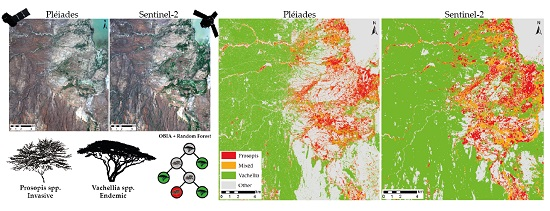
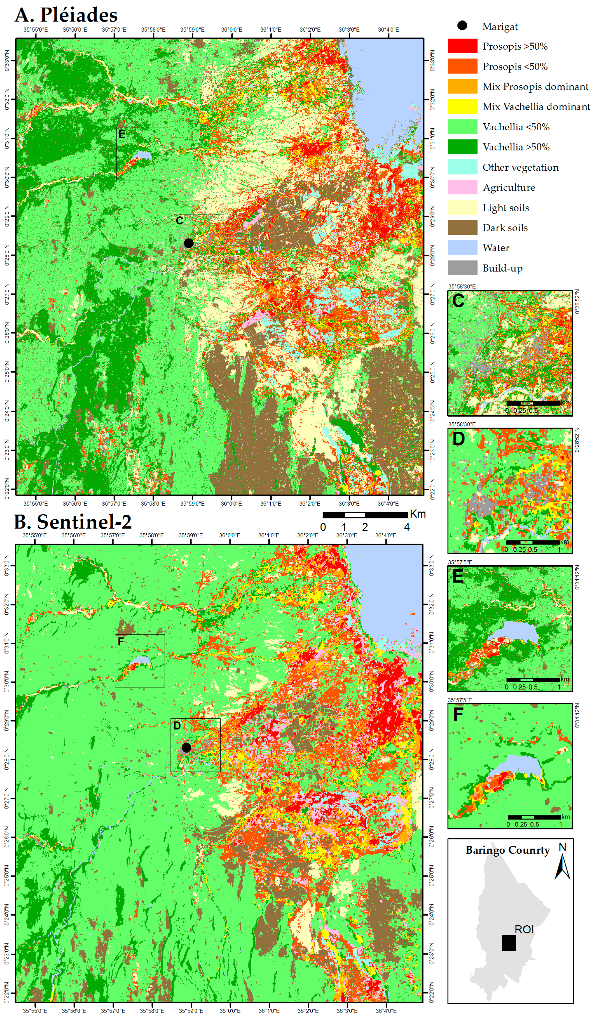
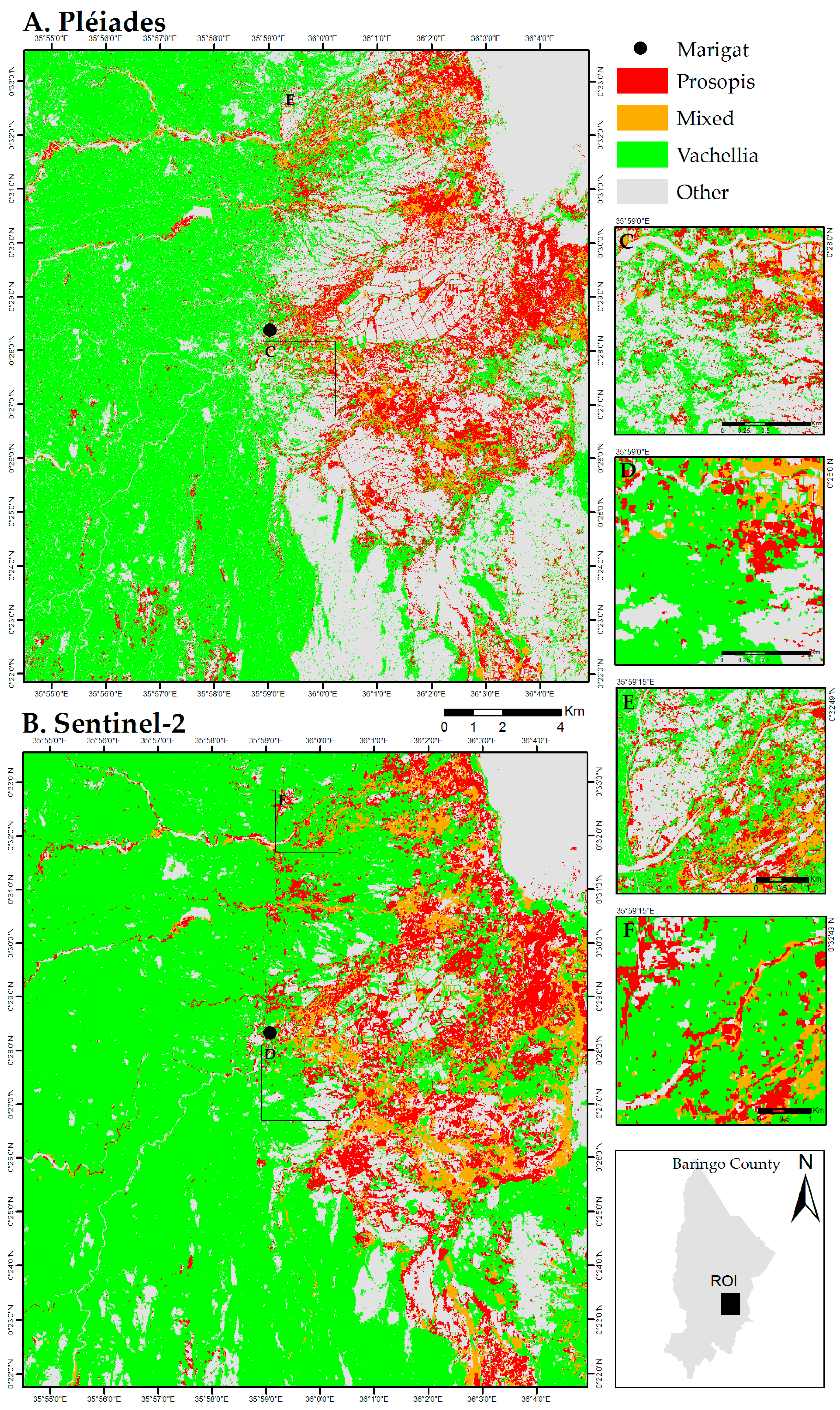
3.1. Prosopis and Vachellia Maps

The 12-class map products of our land cover classifications (Figure 6), display well the situation encountered in the study area and described in the literature [11,94]. Prosopis was found colonizing urban centers (Figure 6C,D) and near waterbodies (Figure 6E,F). The maps also show that the area to the East, which is lower in elevation, highly populated and dominated by agriculture, is heavily invaded by Prosopis. The largest agricultural area (Perkerra irrigation scheme) is classified under agriculture (cropped fields), bare soils (fallow fields) and other vegetation. Prosopis follows, in both classifications, a pattern where it grows along waterbodies and irrigated agricultural areas.
We generalized our results into four broader classes (Section 2.2.2; Table 3) by re-classifying the original land cover classification with twelve classes (Figure 7 and Table 6). Displaying solely the targets for our study, being Prosopis and Vachellia cover, as well as including the areas containing both species (Mixed), and grouping all the non-ProsopisVachellia classes together (Other). The Prosopis, Mixed and Vachellia classes are more abundant in the Sentinel-2 classification (Figure 7B) compared to the Pléiades classification where particularly other non-ProsopisVachellia classes are more frequent (Figure 7A). The spatial distribution of the Mixed class is comparable in both results, however the Sentinel-2 classification indicates higher abundance (Table 6). There appears to be a dissimilarity between class Other in the Pléiades results and class Vachellia in the Sentinel-2 results. The difference is more apparent in lower (east) then higher (west) elevated areas (Figure 7C,D). Finer details are more evident within the Pléiades classification as compared to Sentinel-2 which aggregates small vegetated patches (Figure 7E,F). Notably, Prosopis is apparent along nearly all the rivers in both classification results (Figure 7A,B).
The margin map (Figure 8) was generated by differencing the probabilities of the first (majority vote) and second most often assigned class [95,96]. Values range from 0 to 1 indicating low to high confidence in the attribution to the class. For both datasets the larger Vachellia forest (west), water (Lake Baringo) and the bare agricultural areas receive very high probabilities. On the contrary, some of the sparsely vegetated areas have lowest probability.

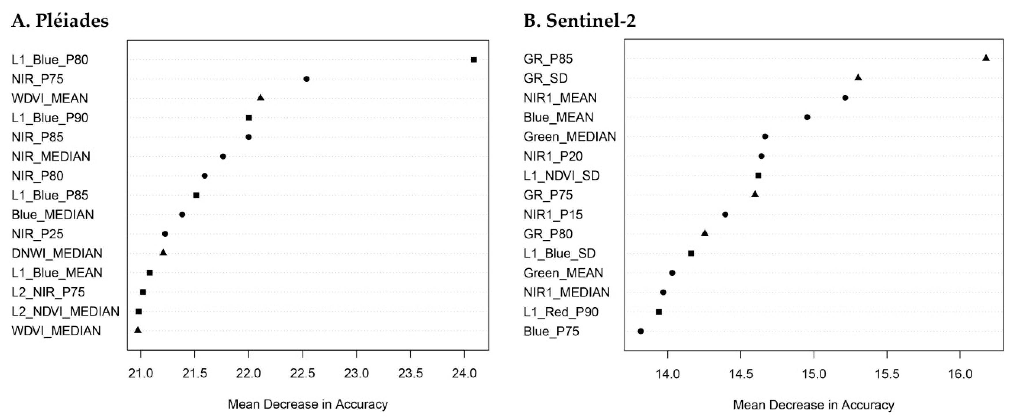
3.2. Feature Importance

The MDA (Figure 9) highlights the feature importance. For each sensor, Figure 9 displays the 15 most important features and differentiates between spectral bands, indices and texture. In both datasets, only seven bands contribute to the 15 most important features. For Pléiades (Figure 9A), the most influential feature is the 80 percentile of the Level 1 wavelets of the blue band. Interestingly, this band appears four more times in the highest ranked feature list. Other significant textural bands for the Pléiades classification are Level 2 NIR and NDVI. The NIR band is also important as it occurs five times in the top ranking features. From the indices only, the DNWI and the WDVI were amongst the top 15. For Sentinel-2 (Figure 9B), the Green Ratio index (GR) generates the highest increases in overall accuracy and appears four times in the list. The most often found spectral bands are blue, green and NIR1. The Level 1 NDVI, blue and red coiflets are also recognized as important textural features.

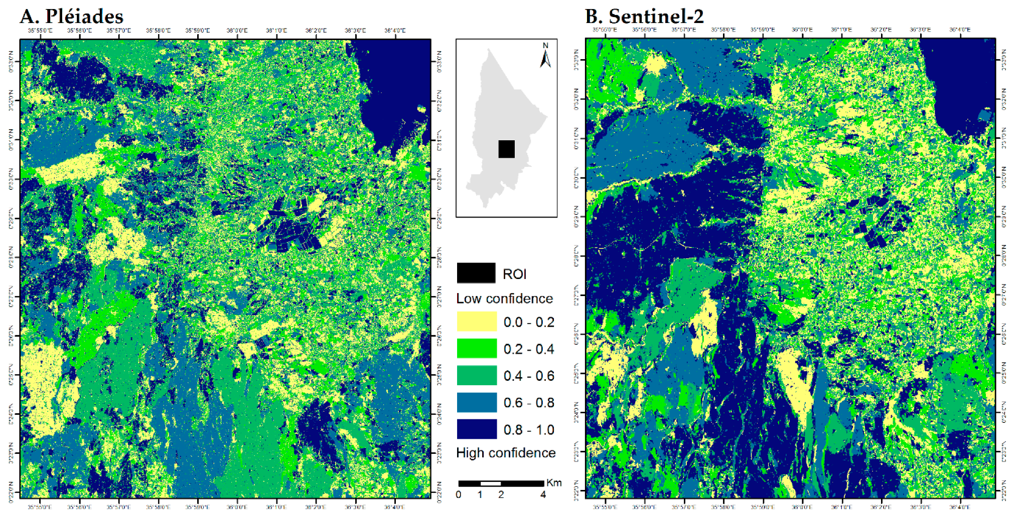
3.3. Accuracy Assessment

Table 7 provides a comprehensive overview of the performed accuracy assessments. The table is divided into Pléiades and Sentinel-2 results and displays the number of independent reference polygons used for the sample count and area proportioned confusion matrices. The area (Wi) depicts the predicted map coverage of each class, while average size shows the area (ha) of the average reference polygon per class. The Out Of Bag (OOB) confusion matrix is provided by the RF classification. To match the OOB matrix to the independent validation we re-classified the 12 classes (Table A1) providing the overall, User’s (Ui), and Producer’s (Pi) accuracies for the four re-classified classes. The sample count shows the overall, Ui and Pi accuracies of the independent validation confusion matrix before area correction. Subsequently, the area proportion presents the area corrected results in terms of overall, Ui and Pi accuracies. All confusion matrices can be found in Table A2.
When assessing the two sensors, Pléiades provides the best overall accuracies for the re-classified map (OOB: 0.91, sample count: 0.88, area prop: 0.95). Sentinel-2 achieves similar results with a higher variability (OOB: 0.85, sample count: 0.79, area prop: 0.96). Most notable differences are the Pléiades for the area proportionate accuracies for the classes Prosopis (Ui: 0.65) and Mix (Pi: 0.58) and for the Sentinel-2 sample count results for Other (Pi: 0.67).
Comparing the validation methods no substantial difference are observed between the OOB, sample count and area proportionate accuracies. Essentially, the area proportionate accuracies are highest and are closely matched with the OOB (second highest accuracy), while the sample count accords for the lowest overall accuracy. Finally, the included information of the validation polygons size and area indicates that the Prosopis and Mixed class mainly consists of small polygons, while the Vachellia and Other class composes of larger polygons dominating the classification results in terms of coverage. The correlation between polygon size and classes is also persisting in the map product.

4. Discussion

4.1. Map Product and Spatial Distribution

The mapped spatial distribution of Prosopis and Vachellia (Figure 7) matches literature [10,26,31] and in situ observations. Prosopis is mainly found at the lowest and wettest areas of the ROI, collecting the majority of runoff water and containing highest population density. Runoff water and density correlate with the amount of cattle, a major disperser and propagator of Prosopis seeds [11]. This is for example illustrated by the abundance of Prosopis: (a) in and near the town centre of Marigat; (b) alongside the roads; (c) surrounding the Perkerra irrigation schemes’ seasonally fallow and grazed fields; and (d) invading free and fertile land made accessible by the retreating water of Lake Baringo.
Vachellia is more abundant on the less populated and steeper slopes of the ROI, which are less utilized and grazed. As there is lower population pressure and disturbance, the established native plant communities prevent Prosopis to invade these areas [15]. As mentioned above, Prosopis is mainly found concentrated along the waterways as described by literature [26,27,31].
Some higher elevated areas along the river beds (west of ROI) surveyed during the fieldwork have no Prosopis. However, the maps indicate some small pockets of Prosopis, these are confused with vegetation which remains evergreen due to its proximity to the river. However, the subdominant evergreen tree species Balanites aegyptiaca, appearing similar to Prosopis, is also found along these riparian zones and the lowlands. Furthermore, we found two sites on the Western slopes where the Prosopis was introduced in a plant breeding effort.

4.2. Map Comparison

Comparing both detailed (12 classes) land cover classifications (Figure 6), we achieved the best mapping results for pure Prosopis and Vachellia on Pléiades data and the sensor has an improved capacity to detect smaller features such as build-up areas. Sentinel-2 provided the best results for the Mixed classes. The overall accuracies (Pléiades: 0.88–0.95; Sentinel-2: 0.79–0.96) are comparable to other studies [26,27,28] and the class specific results are in line and outperform the accuracies (Landsat 8: OOB: 0.71) shown in Ng et al. [28]. Both maps display significant differences in terms of land cover. Visual interpretation of both products suggests the Pléiades map to be of higher accuracy. Several factors contribute to the findings.

4.2.1. Impact of Spatial Resolution

Some differences between the two maps can be attributed to the spatial resolution influencing the object-based results, as described by Immitzer et al. [40,97] and Mirik and Ansley [98]. The differences in resolution, two meters versus ten meters, translated in some of the LSMS polygons consisting in a mix of classes. This affected the Sentinel-2 dataset to a greater extent, resulting in segments containing a mix of soils and sparse vegetation. Obviously, RF will assign a single class to the entire segment, thus homogenizing the polygon and dismissing the other land cover type(s) present within the polygon.
For Baringo, this had a negative impact on the soils and sparsely vegetated Prosopis and Vachellia classes (Pr and Va < 50%), which were classified as either vegetated or bare soils. This outcome originated from the LSMS segmentation, as the parameter selection favors crown detection in dense and mixed stands, while soils, containing a wide ranges of (spectral) information (sands, rocks, wood and shrubs), are segmented into large polygons. This effect increased with decreasing spatial resolution, negatively influencing the Sentinel-2 classification results. In the ten meter resolution dataset, the shrubs and most of the single trees are too small to be detected and fall outside the minimum object size of the LSMS segmentation, set at four pixels (400 m2) (Figure 4). On the contrary, in case of the Pléiades data, its spatial resolution of two meter permits the segmentation to detect and polygonize single tree crowns and allows to distinguish small vegetated patches from soils. The mean polygon sizes (Table 7) demonstrate this issue, showing that the Pléiades segmentation consists of smaller polygons. Furthermore, very large polygons are challenging to establish as reference as they most likely consist of many classes [99]. Furthermore, these huge objects strongly contribute to the variance of the object size distribution [100].

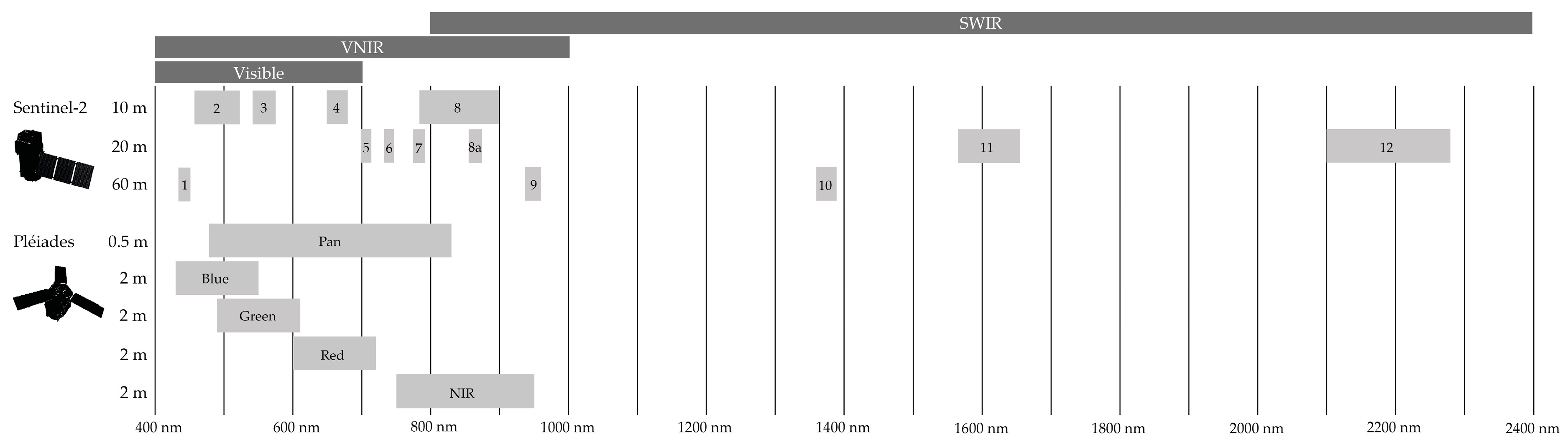
4.2.2. Impact of Spectral Resolution

The spectral resolution had some noticeable influences on the classification results. For the Sentinel-2 data, we could use ten spectral bands, while for the Pléiades we only had four bands at our disposal. This translated into largely different feature sizes when generating the indices and texture parameters. The increased spectral resolution of Sentinel-2 compared to Pléiades partly compensated the pixel size effects and sometimes permitted better OOB accuracies for some classes as described by Immitzer et al. [40] and Duro et al. [101]. This was particularly the case for the area proportionate assessment for the Ui of Mix, Vachellia and Other and the Pi for Prosopis, Vachellia and Other.

4.2.3. Impact of Acquisition Dates

The Pléiades data were acquired one year before the fieldwork and the Sentinel-2 data. The difference has the potential to affect the results [102] as some changes might have happened in classes such as agriculture and bare soils, due to crop rotation and yearly precipitation fluctuations:
  • Pléiades results show for example a higher proportion in the class Other, originating from the soil classes, as compared to Sentinel-2. There could be a relation between the larger exposure of bare soils and the utilization of both Prosopis and Vachellia for charcoal. In the years 2013–2015, the preliminary testing of the Cummins biogas power plant was initiated. The plant was established in Marigat to generate electricity from Prosopis, however, activities were discontinued the next year [103,104]. Hence, the increase in the sparsely vegetated classes in the Sentinel-2 data (2016) could be regrowth of the cleared area.
  • Some of the Prosopis invaded areas visible in the 2015 (Pléiades) data were observed as cleared during the fieldwork. At the same time, some previously none invaded areas (mainly bare soils) had a Prosopis presence when visited in the field. Doing the fieldwork, we were able to determine from the height of Prosopis seedlings that they were half a year old, thus only detectable in one of the datasets (Sentinel-2).
  • The sparsely vegetated Vachellia class and soil classes are often confused, because Vachellia exists as shrubs in some areas due to intense grazing. These misclassifications can be explained by the spectral similarity of Vachellia and the soil classes during the dry season in which the datasets were acquired. During the dry period, being a deciduous tree species, Vachellia is shedding its leaves, thus resembling soil.
  • An additional factor potentially explaining the differences between the class Other and vegetated classes (or soils and sparse vegetation) in 2016, can be attributed to the heavy rainfall coinciding with the 2016 El Niño–Southern Oscillation (ENSO). ENSO is known facilitating fast proliferation of Prosopis and Vachellia [105,106].
  • Observed differences in the Water class are mainly caused by the slowly retreating water level, a consequence of the sudden increase of the water level of Lake Baringo in 2010 [107].
A possible solution for these issues is to either use contemporaneous data or use multi-annual time series [27,108,109].

4.3. Validation and Reference Data

The area proportionate validation, based on the independent reference dataset, indicated overall very high accuracies. The results showed, in contrast to the other accuracy assessment schemes, higher accuracies for the Sentinel-2 maps. We determined that the high in-accuracy of the Pléiades classification persisting in the Ui, is due to the misclassification of large polygons. The effects occurred predominantly in the Prosopis and Mix classes. For example in the Prosopis class 49 polygons (or 86%) were correctly classified and 8 polygons (or 14%) were misclassified. After normalizing the results for map proportion and area, the eight misclassified polygons accounted for 45% while the 49 correctly classified polygons for 55%.
We understand that, to truly independently assess the map accuracy, a more rigorous random sampling scheme needs to be applied. Due to logistical and time constraints, we utilized a set of established sites for validation. The limited number of validation points, providing a confidence level of 85%, was geo-tagged by GPS in the center of preliminary defined field plots. Some of the reference samples indicate low vegetation cover in the inventory’s description, but were actually not vegetated in the satellite data. We observed that some areas were recently cleared, as discussed above. We know from literature that Prosopis seedlings may grow up to one meter and become a shrub within a single year [110,111]. Consequently, the status captured at acquisition date by the satellites and the situation on the ground during field data collection may have changed and forced us to omit the point or substitute it with an adjacent point through orthophoto interpretation.
Another difficulty was the possibility of multiple classes occurring at a given reference sample, as one sample does not necessarily aligns with a single segment created through LSMS. For example, within the 15 m by 15 m Prosopis field plot, and keeping in mind the (in) accuracy of the GPS device, the classes Prosopis, Mixed and Other could all occur, leading to an inconclusive differentiation in the high spatial resolution Pléiades classification. Due to the lower spatial resolution of Sentinel-2, one pixel would cover almost the entire plot. To mitigate this issue we either excluded or moved the point to a nearby area fitting its description. If necessary, this step was performed based on pan-sharpened Pléiades data (0.5 m spatial resolution).

4.4. Random Forest

The robust random forest (RF) classifier provided fast and good results, as established by many studies [28,40,61,78,96]. The processing chain can be easily repeated and applied to other studies with nearly no fine tuning. The feature selection improved our results (not shown) and made it possible to add a large amount of features which were screened for their respective discriminative power. The MDA feature importance (Figure 9) indicated that besides the traditional spectral bands, indices and texture had significant value improving our results. The best 15 features of the Pléiades dataset had for example six spectral bands and wavelets, and three indices. We attribute the lower number of indices to the lack of spectral bands of the sensor. The Sentinel-2 feature importance was more influenced by the spectral data, selecting eight spectral bands, four indices and three wavelets. Interestingly, the two most important features were generated from the GR index. The importance and advantages of indices is well described by the literature [59,61,63,78], while the significance of texture matches the observations of Toscani et al. [76] and Koger et al. [112].

5. Conclusions

In this study, we aimed at producing a highly accurate vegetation type map that differentiates Prosopis from native vegetation types and mixed vegetation classes in a region in Baringo County that is affected by Prosopis invasion. We did this by testing and comparing classification results of two different satellite sensors, Sentinel-2 and Pléiades. The following conclusions can be drawn.
For the Pléiades classification result, features based on the blue and near-infrared band contributed most to the high accuracy, besides features based on vegetation indices. Particularly the level one coiflet of the blue band is considered important. The significance of the blue band was reported by a number of studies [102,113,114]. For the classification based on Sentinel-2, the features based on blue and near-infrared bands were again important, while the green band also contributed significantly. Besides that, Green Ratio—and to a lesser extent—NDVI were important. Overall, recurrent features in both datasets are the blue band, near-infrared band, and coiflet level 1 of the blue band. This demonstrates that the blue band deserves more attention for such vegetation related studies, in particular as the atmospheric correction is nowadays well handled.
The higher spectral resolution of Sentinel-2 on the other hand has a very positive influence on the accuracies, scoring better or equal OOB results of the vegetation classes as the higher spectral information contributes to an improved detection and differentiation of vegetation cover and types.
When comparing the classification results and the achieved class accuracies of both satellite datasets, we can observe that the higher spatial resolution of Pléiades contributes a lot to the level of detail and thus a high accuracy of the derived segmentation and classification result. Particularly, higher OOB and sample count accuracies for classes that are sensitive to the spatial resolution (such as bare soils, sparsely vegetated areas and build-up areas) were obtained.
There are some larger differences in Vachellia cover, attributed to the segmentation process and differences in spatial resolution. The dissimilarities are not between the Prosopis and Vachellia classes but between soils and sparse Vachellia vegetation in the Sentinel-2 data. We therefore conclude that Pléiades data provide the highest class specific accuracy while Sentinel-2 presents the highest map accuracy (area proportionate assessment). The high accuracy correlates with the larger polygons, found in Sentinel-2, and the possibility of classification bias towards large polygons. More research is warranted to investigate the influence of large polygons on classification results.
We also demonstrate that using the free of charge Sentinel-2 data and open source software is a viable alternative achieving promising results (overall accuracy: 0.79–0.96). Further improvements to the parameterization of the Large Scale Mean Shift algorithm could improve the segmentation and classification results. The authors suggest assessing the feasibility of multi-temporal data, which could reveal change dynamics and phenological information, mitigating the bare soils and sparse Vachellia misclassification caused by leaf senescence. Sentinel-2 seems perfectly suited for such kind of study, in particular once the twin satellite is launched (Sentinel-2B) and data are collected at five-day intervals. There is also some potential of incorporating hyper spectral data to better delineate the different tree species.
More research is warranted regarding the invasion pattern of Prosopis since its introduction in the 1980s. A suitable research design is necessary to combine different data sources (e.g., Landsat 5 to 8 with Sentinel-2) and to avoid pitfalls when doing post-classification change detection.

Acknowledgments

This research emerged from a collaborative effort between the University of Natural Resources and Life Sciences, Vienna (BOKU) and the Woody Weeds Project (“Woody invasive alien species in East Africa: Assessing and mitigating their negative impact on ecosystem services and rural livelihood”), which is part of the Swiss Programme for Research on Global Issues for Development (r4d programme) funded jointly by the Swiss Agency for Development and Cooperation (SDC) and the Swiss National Science Foundation (SNSF). We thank the Kenya Forestry Research Institute (KEFRI) and its staff, particularly Simon Choge, for their assistance during the field campaign.

Author Contributions

T.N. and P.R. conceived and designed the experiments; T.N., K.E. and M.I. performed experiments; T.N. and S.E. analyzed the data; and all authors contributed to the writing of the manuscript.

Conflicts of Interest

The authors declare no conflict of interest.

Appendix

Table A1. Confusion matrices of 12-class OOB Pléiades (top) and Sentinel-2 (bottom) classifications.
Pr > 50%Pr < 50%Mix Pr Dominant Mix Va Dominant Va > 50% Va < 50%AgricultureOther VegetationLight SoilsDark SoilsWater Build-upUi
Pr > 50%22130002000000.79
Pr < 50%22601010100000.84
Mix Pr dominant50225002100000.63
Mix Va dominant00518301000000.67
Va > 50%00052300000000.82
Va < 50%00004290002000.83
Agriculture11010023300000.79
Other vegetation02000022300000.85
Light soils00000001290110.91
Dark soils00000001127000.93
Water00000000012900.97
Build-up00000000000291.00
Pi0.730.870.730.600.770.970.770.770.970.900.970.970.83
Pr > 50%Pr < 50%Mix Pr DominantMix Va DominantVa > 50%Va < 50%Agriculture Other VegetationLight SoilsDark SoilsWaterBuild-upUi
Pr > 50%22000007100000.73
Pr < 50%12120024101100.64
Mix Pr dominant20224000000000.79
Mix Va dominant30220500100000.65
Va > 50%00162400000000.77
Va < 50%05111271002000.71
Agriculture21200017001000.74
Other vegetation03000002600000.90
Light soils00000001240030.86
Dark soils00000010025000.96
Water00000000012900.97
Build-up00000100600270.79
Pi0.730.700.730.650.800.900.570.870.800.830.970.900.79
Table A2. Confusion matrices of the four-class OOB, sample count and area proportionate classifications for Pléiades and Sentinel-2.
Pléiades Sentinel-2
ProsopisMixVachelliaOtherUiProsopisMixVachelliaOtherUi
OOB accuracyProsopis513130.8794402150.721
Mix550340.806548510.814
Vachellia055620.889595230.754
Other4101710.9726211610.947
Pi0.8500.8470.9330.9500.9140.7330.8140.8670.8940.850
Pléiades Sentinel-2
ProsopisMixVachelliaOtherUiProsopisMixVachelliaOtherUi
Sample countProsopis497130.8174432140.698
Mix133000.971940510.727
Vachellia056320.900215790.826
Other702680.883212490.907
Pi0.8600.7330.9550.9320.8840.7720.8890.8640.6710.788
Pléiades Sentinel-2
ProsopisMixVachelliaOtherUiProsopisMix VachelliaOtherUi
Area sumProsopis105,57635,28036822,1360.646201,4003400610037,1000.812
Mix384125,584000.99753,800595,30016,30083,6000.795
Vachellia063,40831,731,78617,2520.99711,2006004,7547,100127,9000.997
Other84,5680388,16018,254,2840.97514,900600520013,728,3000.998
Pi0.5540.5600.9880.9980.9880.7160.9920.9990.9820.994
Pléiades Sentinel-2
ProsopisMixVachelliaOtherUiProsopisMixVachellia OtherUi
Area proportionatProsopis0.0710.0240.0000.0150.6460.0950.0020.0030.0170.812
Mix0.0000.0350.0000.0000.9970.0040.0470.0010.0070.795
Vachellia0.0000.0010.4720.0000.9970.0000.0000.6270.0020.997
Other0.0020.0000.0080.3730.9750.0000.0000.0000.1960.998
Pi0.9750.5830.9830.9610.9500.9540.9670.9930.8840.964

References

  1. Kariuki, P. A Social Forestry Project in Baringo, Kenya: A Critical Analysis; University of Queensland: Brisbane, Autralia, 1993. [Google Scholar]
  2. Shackleton, R.T.; Le Maitre, D.C.; Pasiecznik, N.M.; Richardson, D.M. Prosopis: A global assessment of the biogeography, benefits, impacts and management of one of the world’s worst woody invasive plant taxa. AoB Plants 2014, 6, 1–18. [Google Scholar] [CrossRef] [PubMed]
  3. Shiferaw, H.; Teketay, D.; Nemomissa, S.; Assefa, F. Some biological characteristics that foster the invasion of Prosopis juliflora (Sw.) DC. at Middle Awash Rift Valley Area, north-eastern Ethiopia. J. Arid Environ. 2004, 58, 135–154. [Google Scholar] [CrossRef]
  4. Felker, P. Mesquite: An all purpose leguminous arid land tree. In New Agricultural Crops, American Association for the Advancement of Science Symposium; Ritchie, G.A., Ed.; Westview Press: Boulder, UT, USA, 1979; Volume 38, pp. 89–132. [Google Scholar]
  5. Forsyth, G.G.; Le Maitre, D.C.; O’Farrell, P.J.; van Wilgen, B.W. The prioritisation of invasive alien plant control projects using a multi-criteria decision model informed by stakeholder input and spatial data. J. Environ. Manag. 2012, 103, 51–57. [Google Scholar] [CrossRef] [PubMed]
  6. Nilsen, E.T.; Sharifi, M.R.; Rundel, P.W.; Jarrell, W.M.; Virginia, R.A. Diurnal and seasonal water relations of the desert phreatophyte Prosopis glandulosa (honey mesquite) in the Sonoran Desert of California. Ecology 1983, 64, 1381–1393. [Google Scholar] [CrossRef]
  7. Dzikiti, S.; Schachtschneider, K.; Naiken, V.; Gush, M.; Moses, G.; Le Maitre, D.C. Water relations and the effects of clearing invasive Prosopis trees on groundwater in an arid environment in the northern Cape, South Africa. J. Arid Environ. 2013, 90, 103–113. [Google Scholar] [CrossRef]
  8. Elfadl, M.A.; Luukkanen, O. Ecological strategies of Prosopis juliflora in the arid environment of the Sudan: 1. Leaf gas exchange approach. J. Arid Environ. 2006, 66, 1–15. [Google Scholar] [CrossRef]
  9. Lenachuru, C. Impacts of Prosopis species in Baringo District. In Proceedings of workshop on Integrated Management of Prosopis Species in Kenya, Nairobi, Kenya, 1–2 October 2003. [CrossRef]
  10. Andersson, S. Spread of the Introduced Tree Species Prosopis juliflora (Sw.) DC in the Lake Baringo Area, Kenya. Ph.D. Thesis, Faculty of Forest Sciences, Swedish University of Agricultural Sciences, Umeå, Sweden, 2005. [Google Scholar]
  11. Pasiecznik, N.; Felker, P.; Cadoret, K.; Harsh, L.N.; Cruz, G.; Tewari, J.C.; Maldonado, L.J. The Prosopis juliflora-Prosopis pallida complex: The Prosopis juliflora-Prosopis pallida complex. Managing 2001, 231, 162. [Google Scholar]
  12. Lowe, S.; Browne, M.; Boudjelas, S.; De Poorter, M. 100 of the World’s Worst Invasive Alien Species: A Selection from the Global Invasive Species Database; Invasive Species Specialist Group a Specialist Group Species Survival Commission of the World Conservation Union: Auckland, New Zealand, 2000. [Google Scholar]
  13. Maslin, B.R. Generic and subgeneric names in Acacia following retypification of the genus. Muelleria 2008, 26, 7–9. [Google Scholar]
  14. Groot, H.; Hall, D. How to pick crops that cope with extreme climates. In New Scientist; Reed Business Information Ltd.: London, UK, 1989; pp. 46–47. [Google Scholar]
  15. Burke, M.J.W.; Grime, J.P. An experimental study of plant community invasibility. Ecology 1996, 77, 776–790. [Google Scholar] [CrossRef]
  16. Yoda, K.; Elbasit, M.A.; Hoshino, B.; Nawata, H.; Yasuda, H. Root system development of Prosopis seedlings under different soil moisture conditions. J. Arid Land Stud. 2012, 16, 13–16. [Google Scholar]
  17. Aboud, A.A.; Kisoyan, P.K.; Coppock, D.L. Agro-pastoralists’ wrath for the Prosopis tree: The Case of the Il Chamus of Baringo district, Kenya. In Global Livestock Collaborative Research Support Program; ENVS Faculty Publications: Davis, CA, USA, 2005; pp. 1–3. [Google Scholar]
  18. Geesing, D.; Al-Khawlani, M.; Abba, M.L. Management of introduced Prosopis species: Can economic exploitation control an invasive species? Unasylva 2004, 55, 36–44. [Google Scholar]
  19. Sawal, R.K.; Ram, R.; Yadav, S.B.S. Mesquite (Prosopis juliflora) pods as a feed resource for livestock—A review. Asian-Aust. J. Anim. Sci. 2004, 17, 719–725. [Google Scholar] [CrossRef]
  20. Peter, F.F.; Thames, J.L. Collection, Handling, Storage and Pre-treatment of Prosopis Seeds in Latin America; FAO: Rome, Italy, 1983. [Google Scholar]
  21. Orwa, C.; Mutua, A.; Kindt, R.; Jamnadass, R.; Anthony, S. Agroforestree Database: A Tree Reference and Selection Guide Version 4.0. Available online: http://www.worldagroforestry.org/output/agroforestree-database (accessed on 6 January 2017).
  22. Guevara, A.; Giordano, C.V.; Aranibar, J.; Quiroga, M.; Villagra, P.E. Phenotypic plasticity of the coarse root system of Prosopis flexuosa, a phreatophyte tree, in the Monte Desert (Argentina). Plant Soil 2010, 330, 447–464. [Google Scholar] [CrossRef]
  23. Seghieri, J. The rooting patterns of woody and herbaceous plants in a savanna; Are they complementary or in competition? Afr. J. Ecol. 1995, 33, 358–365. [Google Scholar] [CrossRef]
  24. Aplin, P. Remote sensing: Ecology. Prog. Phys. Geogr. 2005, 29, 104–113. [Google Scholar] [CrossRef]
  25. Huang, C.Y.; Asner, G.P. Applications of remote sensing to alien invasive plant studies. Sensors 2009, 9, 4869–4889. [Google Scholar] [CrossRef] [PubMed]
  26. Rembold, F.; Leonardi, U.; Ng, W.; Gadain, H.; Meroni, M. Mapping areas invaded by Prosopis juliflora in Somaliland with Landsat 8 imagery. Proc. SPIE 2015, 9637, 1–12. [Google Scholar]
  27. Meroni, M.; Ng, W.-T.; Rembold, F.; Leonardi, U.; Atzberger, C.; Gadain, H.; Shaiye, M. Mapping Prosopis juliflora in west Somaliland with Landsat 8 satellite imagery and ground information. Land Degrad. Dev. 2016. [Google Scholar] [CrossRef]
  28. Ng, W.-T.; Meroni, M.; Immitzer, M.; Böck, S.; Leonardi, U.; Rembold, F.; Gadain, H.; Atzberger, C. Mapping Prosopis spp. with Landsat 8 data in arid environments: Evaluating effectiveness of different methods and temporal imagery selection for Hargeisa, Somaliland. Int. J. Appl. Earth Obs. Geoinf. 2016, 53, 76–89. [Google Scholar] [CrossRef]
  29. Wakie, T.T.; Evangelista, P.H.; Jarnevich, C.S.; Laituri, M. Mapping current and potential distribution of non-native Prosopis juliflora in the Afar Region of Ethiopia. PLoS ONE 2014, 9, 1–9. [Google Scholar] [CrossRef] [PubMed]
  30. Ayanu, Y.; Jentsch, A.; Müller-Mahn, D.; Rettberg, S.; Romankiewicz, C.; Koellner, T. Ecosystem engineer unleashed: Prosopis juliflora threatening ecosystem services? Reg. Environ. Chang. 2014, 15, 155–167. [Google Scholar] [CrossRef]
  31. Van Den Berg, E.C.; Kotze, I.; Beukes, H. Detection, quantification and monitoring Prosopis spp. in the Northern Cape Province of South Africa using remote sensing and GIS. South Afr. J. Geomatic. 2013, 2, 68–81. [Google Scholar]
  32. Robinson, T.P.; Wardell-Johnson, G.W.; Pracilio, G.; Brown, C.; Corner, R.; van Klinken, R.D. Testing the discrimination and detection limits of WorldView-2 imagery on a challenging invasive plant target. Int. J. Appl. Earth Obs. Geoinf. 2016, 44, 23–30. [Google Scholar] [CrossRef]
  33. Muturi, G.M.; Poorter, L.; Mohren, G.M.J.; Kigomo, B.N. Ecological impact of Prosopis species invasion in Turkwel riverine forest, Kenya. J. Arid Environ. 2013, 92, 89–97. [Google Scholar] [CrossRef]
  34. Dubow, A.Z. Mapping and Managing the Spread of Prosopis Juliflora in Garissa County, Kenya. Master’s Thesis, School of Environmental Studies of Kenyatta University, Nairobi, Kenya, 2011; p. 80. [Google Scholar]
  35. Amboka, A.A.; Ngigi, T.G. Mapping and monitoring spatial-temporal cover change of Prosopis species colonization in Baringo Central, Kenya. Int. J. Eng. Sci. Invent. 2015, 4, 2319–6734. [Google Scholar]
  36. Swallow, B.; Mwangi, E. Invasion and rural livelihoods in the Lake Baringo area of Kenya. Conserv. Soc. 2008, 6, 130. [Google Scholar] [CrossRef]
  37. Thenkabail, P.S. Land Resources Monitoring, Modeling, and Mapping with Remote Sensing; CRC Press: Boca Raton, FL, USA, 2015. [Google Scholar]
  38. Alsharrah, S.A.; Bruce, D.A.; Bouabid, R.; Somenahalli, S.; Corcoran, P.A. High-spatial resolution multispectral and panchromatic satellite imagery for mapping perennial desert plants. Proc. SPIE 2015, 9644. [Google Scholar] [CrossRef]
  39. Regniers, O.; Bombrun, L.; Guyon, D.; Samalens, J.C.; Germain, C. Wavelet-based texture features for the classification of age classes in a maritime pine forest. IEEE Geosci. Remote Sens. Lett. 2015, 12, 621–625. [Google Scholar] [CrossRef]
  40. Immitzer, M.; Vuolo, F.; Atzberger, C. First experience with Sentinel-2 data for crop and tree species classifications in Central Europe. Remote Sens. 2016, 8, 166. [Google Scholar] [CrossRef]
  41. Radoux, J.; Chomé, G.; Jacques, D.C.; Waldner, F.; Bellemans, N.; Matton, N.; Lamarche, C.; d’Andrimont, R.; Defourny, P. Sentinel-2’s potential for sub-pixel landscape feature detection. Remote Sens. 2016, 8, 488. [Google Scholar] [CrossRef]
  42. Pratt, D.; Gwynne, M. Rangeland Management and Ecology in East Africa; Hodder & Stoughton: London, UK, 1977. [Google Scholar]
  43. Thom, D.; Martin, N. Ecology and production in Baringo-Kerio Valley, Kenya. Geogr. Rev. 1983, 73, 15–29. [Google Scholar] [CrossRef]
  44. Meroni, M.; Verstraete, M.M.; Rembold, F.; Urbano, F.; Kayitakire, F. A phenology-based method to derive biomass production anomalies for food security monitoring in the Horn of Africa. Int. J. Remote Sens. 2014, 35, 2472–2492. [Google Scholar] [CrossRef]
  45. Wiesmann, U.; Kiteme, B.; Mwangi, Z. Socio-Economic Atlas of Kenya: Depicting the National Population Census by County and Sub-Location, 2nd ed.; KNBS: Nairobi, Kenya; CETRAD: Nanyuki, Kenya; CDE: Bern, Switherland, 2016. [Google Scholar]
  46. Geosystems. Erdas imagine. Imagine 2005, 15, 1–16. [Google Scholar]
  47. Main-Knorn, M.; Pflug, B.; Debaecker, V.; Louis, J. Calibration and validation plan for the L2a processor and products of the Sentinel-2 mission. ISPRS Int. Arch. Photogramm. Remote Sens. Spat. Inf. Sci. 2015, 40, 1249–1255. [Google Scholar] [CrossRef]
  48. Vuolo, F.; Żółtak, M.; Pipitone, C.; Zappa, L.; Wenng, H.; Immitzer, M.; Weiss, M.; Baret, F.; Atzberger, C. Data service platform for Sentinel-2 surface reflectance and value-added products: System use and examples. Remote Sens. 2016, 8, 938. [Google Scholar] [CrossRef]
  49. Inglada, J.; Christophe, E. The Orfeo Toolbox remote sensing image processing software. In Proceedings of 2009 IEEE International Geoscience and Remote Sensing Symposium, Cape Town, South Africa, 12–17 July 2009; pp. 733–736.
  50. Harrington, M.; Cross, M. Google Earth Forensics; Elsevier: Waltham, MA, USA, 2015. [Google Scholar]
  51. Woody Weeds Project. Available online: http://woodyweeds.org/ (accessed on 4 January 2017).
  52. Blaschke, T. Object based image analysis for remote sensing. ISPRS J. Photogramm. Remote Sens. 2010, 65, 2–16. [Google Scholar] [CrossRef]
  53. Blaschke, T.; Hay, G.J.; Kelly, M.; Lang, S.; Hofmann, P.; Addink, E.; Feitosa, R.Q.; van der Meer, F.; van der Werff, H.; van Coillie, F.; et al. Geographic object-based image analysis—Towards a new paradigm. ISPRS J. Photogramm. Remote Sens. 2014, 87, 180–191. [Google Scholar] [CrossRef] [PubMed]
  54. Fukunaga, K.; Hostetler, L. The estimation of the gradient of a density function, with applications in pattern recognition. IEEE Trans. Inf. Theory 1975, 21, 32–40. [Google Scholar] [CrossRef]
  55. Comaniciu, D.; Meer, P. Mean shift: A robust approach toward feature space analysis. IEEE Trans. Pattern Anal. Mach. 2002, 24, 603–619. [Google Scholar] [CrossRef]
  56. Michel, J.; Youssefi, D.; Grizonnet, M. Stable mean-shift algorithm and its application to the segmentation of arbitrarily large remote sensing images. IEEE Trans. Geosci. Remote Sens. 2015, 53, 952–964. [Google Scholar] [CrossRef]
  57. Huang, X.H.X.; Zhang, L.Z.L. An adaptive mean-shift analysis approach for object extraction and classification from urban hyperspectral imagery. IEEE Trans. Geosci. Remote Sens. 2008, 46, 4173–4185. [Google Scholar] [CrossRef]
  58. Pouliot, D.A.; King, D.J.; Bell, F.W.; Pitt, D.G. Automated tree crown detection and delineation in high-resolution digital camera imagery of coniferous forest regeneration. Remote Sens. Environ. 2002, 82, 322–334. [Google Scholar] [CrossRef]
  59. Waser, L.T.; Küchler, M.; Jütte, K.; Stampfer, T. Evaluating the potential of WorldView-2 data to classify tree species and different levels of ash mortality. Remote Sens. 2014, 6, 4515–4545. [Google Scholar] [CrossRef]
  60. Gitelson, A.A.; Kaufman, Y.J.; Merzlyak, M.N. Use of a green channel in remote sensing of global vegetation from EOS-MODIS. Remote Sens. Environ. 1996, 58, 289–298. [Google Scholar] [CrossRef]
  61. Immitzer, M.; Atzberger, C. Early detection of Bark Beetle Infestation in Norway Spruce (Picea abies, L.) using WorldView-2 Data. Photogramm. Fernerkund. Geoinf. 2014, 5, 351–367. [Google Scholar] [CrossRef]
  62. Qi, J.; Chehbouni, A.; Huete, A.R.; Kerr, Y.H.; Sorooshian, S. A modified soil adjusted vegetation index. Remote Sens. Environ. 1994, 48, 119–126. [Google Scholar] [CrossRef]
  63. Gitelson, A.; Merzlyak, M.N. Quantitative estimation of chlorophyll-a using reflectance spectra: Experiments with autumn chestnut and maple leaves. J. Photochem. Photobiol. B Biol. 1994, 22, 247–252. [Google Scholar] [CrossRef]
  64. Barnes, E.; Clarke, T.; Richards, S.; Colaizzi, P.D.; Haberland, J.; Kostrzewski, M.; Waller, P.; Choi, C.; Riley, E.; Thompson, T.; et al. Coincident detection of crop water stress, nitrogen status and canopy density using ground-based multispectral data. In Proceedings of the 5th International Conference on Precision Agriculture, Bloomington, MN, USA, 16–19 July 2000.
  65. Rouse, J.W.; Haas, R.H.; Schell, J.A.; Deering, D.W. Monitoring vegetation systems in the Great Plains with ERTS. In Proceedings of Third Earth Resources Technology Satellite-1 Symposium, Washington, DC, USA, 10–14 December 1973; pp. 309–317.
  66. Gao, B.C. NDWI—A normalized difference water index for remote sensing of vegetation liquid water from space. Remote Sens. Environ. 1996, 58, 257–266. [Google Scholar] [CrossRef]
  67. Sripada, R.P.; Heiniger, R.W.; White, J.G.; Meijer, A.D. Aerial color infrared photography for determining early in-season nitrogen requirements in corn. Agron. J. 2006, 98, 968–977. [Google Scholar] [CrossRef]
  68. Merzlyak, M.N.; Gitelson, A.A.; Chivkunova, O.B.; Rakitin, V.Y.U. Non-destructive optical detection of pigment changes during leaf senescence and fruit ripening. Physiol. Plant. 1999, 106, 135–141. [Google Scholar] [CrossRef]
  69. Jordan, C.F. Derivation of leaf-area index from quality of light on the forest floor. Ecology 1969, 50, 663–666. [Google Scholar] [CrossRef]
  70. Pearson, R.L.; Miller, L.D. Remote mapping of standing crop biomass for estimation of the productivity of the short-grass Prairie, Pawnee National Grassland, Colorado. In Proceedings of Eighth International Symposium on Remote Sensing of Environment, Ann Arbor, MI, USA, 2–6 October 1972; pp. 1357–1381.
  71. Walz, U.; Hou, W. Charakterisierung der Landschaftsvielfalt mit RapidEye-Daten—Erste Ergebnisse und Erfahrungen. In Proceedings of the 3 RESA Workshop, Neustrelitz, Germany, 23 March 2011; pp. 75–85.
  72. Chávez, R.; Clevers, J.G.P.W. Phase 2. In Object-Based Analysis of 8-Bands WorldView-2 Imagery for Assessing Health Condition of Desert Trees, 8-Band Research Challenge; Digital Globe of Longmont: Westminster, CO, USA, 2011; pp. 1–8. [Google Scholar]
  73. Richardson, A.J.; Wiegand, C.L. Distinguishing vegetation from soil background information. Photogramm. Eng. Remote Sens. 1977, 43, 1541–1552. [Google Scholar]
  74. Clevers, J.G.P.W. The derivation of a simplified reflectance model for the estimation of leaf area index. Remote Sens. Environ. 1988, 25, 53–69. [Google Scholar] [CrossRef]
  75. Wolf, A.F. Using WorldView-2 Vis-NIR multispectral imagery to support land mapping and feature extraction using normalized difference index ratios. Proc. SPIE 2012, 8390. [Google Scholar] [CrossRef]
  76. Toscani, P.; Immitzer, M.; Atzberger, C. Wavelet-based texture measures for object-based classification of aerial images. Photogramm. Fernerkund. Geoinf. 2013, 2013, 105–121. [Google Scholar] [CrossRef]
  77. Huang, X.; Zhang, L. An SVM ensemble approach combining spectral, structural, and semantic features for the classification of high-resolution remotely sensed imagery. IEEE Trans. Geosci. Remote Sens. 2013, 51, 257–272. [Google Scholar] [CrossRef]
  78. Immitzer, M.; Atzberger, C.; Koukal, T. Tree species classification with random forest using very high spatial resolution 8-Band WorldView-2 satellite data. Remote Sens. 2012, 4, 2661–2693. [Google Scholar] [CrossRef]
  79. Huang, X.; Zhang, L.; Wang, L. Evaluation of morphological texture features for mangrove forest mapping and species discrimination using multispectral IKONOS imagery. IEEE Geosci. Remote Sens. Lett. 2009, 6, 393–397. [Google Scholar] [CrossRef]
  80. Daubechies, I. Ten Lectures on Wavelets; SIAM: Philadelphia, PA, USA, 1992; Volume 61. [Google Scholar]
  81. MATLAB R2012a, version 7.10.0; The MathWorks Inc.: Natick, MA, USA, 2010.
  82. Breiman, L. Random forests. Mach. Learn. 2001, 45, 5–32. [Google Scholar] [CrossRef]
  83. Hastie, T.; Tibshirani, R.; Friedman, J. The Elements of Statistical Learning: Data Mining, Inference, and Prediction; Springer: Berlin, Germany, 2009. [Google Scholar]
  84. Gislason, P.O.; Benediktsson, J.A.; Sveinsson, J.R. Random forests for land cover classification. Pattern Recognit. Lett. 2006, 27, 294–300. [Google Scholar] [CrossRef]
  85. Li, X.; Cheng, X.; Chen, W.; Chen, G.; Liu, S. Identification of forested landslides using LiDar data, object-based image analysis, and machine learning algorithms. Remote Sens. 2015, 7, 9705–9726. [Google Scholar] [CrossRef]
  86. Li, X.; Chen, W.; Cheng, X.; Wang, L. A comparison of machine learning algorithms for mapping of complex surface-mined and agricultural landscapes using ZiYuan-3 stereo satellite imagery. Remote Sens. 2016, 8, 514. [Google Scholar] [CrossRef]
  87. Liaw, A.; Wiener, M. Classification and regression by randomForest. R News 2002, 2, 18–22. [Google Scholar]
  88. R Core Team. R: A Language and Environment for Statistical Computing; R Foundation for Statistical Computing: Vienna, Austria, 2015. [Google Scholar]
  89. Genuer, R.; Poggi, J.-M.; Tuleau-Malot, C. Variable selection using random forests. Pattern Recognit. Lett. 2010, 31, 2225–2236. [Google Scholar] [CrossRef]
  90. Congalton, R.G.; Green, K. Assessing the Accuracy of Remotely Sensed Data: Principles and Practices; CRC Press: Boca Raton, FL, USA, 2009; Volume 2. [Google Scholar]
  91. Olofsson, P.; Foody, G.M.; Herold, M.; Stehman, S.V.; Woodcock, C.E.; Wulder, M.A. Good practices for estimating area and assessing accuracy of land change. Remote Sens. Environ. 2014, 148, 42–57. [Google Scholar] [CrossRef]
  92. Stehman, S.V. Estimating area from an accuracy assessment error matrix. Remote Sens. Environ. 2013, 132, 202–211. [Google Scholar] [CrossRef]
  93. Radoux, J.; Bogaert, P. Accounting for the area of polygon sampling units for the prediction of primary accuracy assessment indices. Remote Sens. Environ. 2014, 142, 9–19. [Google Scholar] [CrossRef]
  94. Rembold, F.; Atzberger, C.; Savin, I.; Rojas, O. Using low resolution satellite imagery for yield prediction and yield anomaly detection. Remote Sens. 2013, 5, 1704–1733. [Google Scholar] [CrossRef] [Green Version]
  95. Vuolo, F.; Atzberger, C. Improving land cover maps in areas of disagreement of existing products using NDVI time series of MODIS—Example for Europe. Photogramm. Fernerkund. Geoinf. 2014, 201, 393–407. [Google Scholar] [CrossRef]
  96. Schultz, B.; Immitzer, M.; Formaggio, A.R.; Sanches, I.D.A.; Luiz, A.J.B.; Atzberger, C. Self-guided segmentation and classification of multi-temporal Landsat 8 images for crop type mapping in Southeastern Brazil. Remote Sens. 2015, 7, 14482–14508. [Google Scholar] [CrossRef]
  97. Immitzer, M.; Vuolo, F.; Einzmann, K.; Ng, W.-T.; Böck, S.; Atzberger, C. Verwendung von multispektralen Sentinel-2 Daten für die Baumartenklassifikation und Vergleich mit anderen Satellitensensoren. In Proceedings of Conferemce Dreiländertagung der SGPF, DGPF und OVG, Bern, Switzerland, 8–9 June 2016; Volume 25, pp. 417–427.
  98. Mirik, M.; Ansley, R.J. Utility of satellite and aerial images for quantification of canopy cover and infilling rates of the invasive woody species honey mesquite (Prosopis Glandulosa) on Rangeland. Remote Sens. 2012, 4, 1947–1962. [Google Scholar] [CrossRef]
  99. Stehman, S.V.; Wickham, J.D. Pixels, blocks of pixels, and polygons: Choosing a spatial unit for thematic accuracy assessment. Remote Sens. Environ. 2011, 115, 3044–3055. [Google Scholar] [CrossRef]
  100. Radoux, J.; Bogaert, P.; Fasbender, D.; Defourny, P. Thematic accuracy assessment of geographic object-based image classification. Int. J. Geogr. Inf. Sci. 2011, 25, 895–911. [Google Scholar] [CrossRef]
  101. Duro, D.C.; Franklin, S.E.; Dubé, M.G. A comparison of pixel-based and object-based image analysis with selected machine learning algorithms for the classification of agricultural landscapes using SPOT-5 HRG imagery. Remote Sens. Environ. 2012, 118, 259–272. [Google Scholar] [CrossRef]
  102. Fassnacht, F.E.; Latifi, H.; Stereńczak, K.; Modzelewska, A.; Lefsky, M.; Waser, L.T.; Staub, C.; Ghosh, A. Review of studies on tree species classification from remotely sensed data. Remote Sens. Environ. 2016, 186, 64–87. [Google Scholar] [CrossRef]
  103. US Embassy Cummins Cogeneration Kenya Limited (CCKL) 12MW Biomass-Fueled, On-Grid Electricity Generation Project in Baringo County, Kenya. Available online: http://nairobi.usembassy.gov/cumminsbaringo.html (accessed on 5 January 2017).
  104. Cummins Power Generation. Cummins Power Generation Project in Kenya Paves the Way for African Biogas Expansion. Available online: http://www.cumminspowerblog.com/en/2014/08/27/cummins-power-generation-project-kenya-paves-way-african-biogas-expansion/ (accessed on 5 January 2017).
  105. Red Cross Kenya. Situation Report of Effects of the El Nino Rains; Red Cross Kenya: Nairobi, Kenya, 2015. [Google Scholar]
  106. Rui, H.; McNally, A. Famine Early Warning Systems Network (FEWS NET) Land Data Assimilation System (FLDAS) Product; USGS Center for Earth Resources Observation and Science (EROS): Sioux Falls, SD, USA, 2015.
  107. Obando, J.; Onywere, S.; Shisanya, C.; Nbudi, A.; Masiga, D.; Irura, Z.; Mariita, N.; Maragia, H. Impact of short-term flooding on livelihoods in the Kenya Rift Valley Lakes. In Advances in Geographical and Environmental Sciences; Springer: Tokyo, Japan, 2016; pp. 193–215. [Google Scholar]
  108. Schmidt, T.; Schuster, C.; Kleinschmit, B.; Förster, M. Evaluating an intra-annual time series for grassland classification—How many acquisitions and what seasonal origin are optimal? IEEE J. Sel. Top. Appl. Earth Obs. Remote Sens. 2014, 7, 3428–3439. [Google Scholar] [CrossRef]
  109. Vuolo, F.; Richter, K.; Atzberger, C. Evaluation of time-series and phenological indicators for land cover classification based on MODIS data. Proc. SPIE 2011. [Google Scholar] [CrossRef]
  110. Elfadl, M.A. Growth performance and physiological characteristics of seedlings of six tropical dry. J. Nat. Resour. Environ. Stud. 2013, 1, 25–33. [Google Scholar]
  111. Muthana, K.D.; Arora, G.D. Prosopis juliflora (Swartz) DC, a fast growing tree to bloom the desert. In Central Arid Zone Research Institute Monograph; Central Arid Zone Research Institute: Jodhpur, India, 1983; Volume 22, pp. 1–19. [Google Scholar]
  112. Koger, C.H.; Bruce, L.M.; Shaw, D.R.; Reddy, K.N. Wavelet analysis of hyperspectral reflectance data for detecting pitted morningglory (Ipomoea lacunosa) in soybean (Glycine max). Remote Sens. Environ. 2003, 86, 108–119. [Google Scholar] [CrossRef]
  113. Peerbhay, K.Y.; Mutanga, O.; Ismail, R. Investigating the capability of few strategically placed WorldView-2 multispectral bands to discriminate forest species in KwaZulu-Natal, South Africa. IEEE J. Sel. Top. Appl. Earth Obs. Remote Sens. 2014, 7, 307–316. [Google Scholar] [CrossRef]
  114. Pu, R.; Liu, D. Segmented canonical discriminant analysis of in situ hyperspectral data for identifying 13 urban tree species. Int. J. Remote Sens. 2011, 32, 2207–2226. [Google Scholar] [CrossRef]
Figure 1. Generalization of the adaptations of Prosopis (left) and Vachellia (right) spp. [11,16,22,23], summarizing the competitive advantages of Prosopis in seed production, root system, leaf and pod palatability.
Remotesensing 09 00074 g001
Figure 2. Pan-sharpened true color Pléiades image (using subtractive resolution merge in Erdas Imagine [46]) of the study area centered around Marigat (left), including the Prosopis plantations [10] and in situ collected reference dataset used for training the classifier. Map of Kenya (upper right) with location of ROI and Digital Elevation Model (lower right) generated from Pléiades stereo imagery along with roads and waterways.
Remotesensing 09 00074 g002
Figure 3. Overview of spectral and spatial resolution of Sentinel-2 and Pléiades.
Remotesensing 09 00074 g003
Figure 4. Comparison of false color data with segmentation results of the Large Scale Mean Shift algorithm (in yellow). A digitized tree crown (ingreen) is also shown: (A) pan-sharpened Pléiades data; (B) original Pléiades data; and (C) Sentinel-2 data. The parameter selection used for the LSMS segmentation is displayed in Table 4.
Remotesensing 09 00074 g004
Figure 5. Workflow describing the classification process for both Pléiades and Sentinel-2 dataset.
Remotesensing 09 00074 g005
Figure 6. Results of the object-based land cover classification of the study area: (A) Pléiades; (B) Sentinel-2. Captions displayl (C,D) Prosopis invasion in the urban area of Marigat; and (E,F) Prosopis invading a small waterbody.
Remotesensing 09 00074 g006
Figure 7. Classification results including Prosopis, Vachellia, Mixed and Other illustrating: (A) the Pléiades results; (B) the Sentinel-2 results; and comparisons between both sensors in respect of differences in classification (C,D); and detection of small vegetated patches (E,F). For definition of the re-classified (broad) classes, refer to Table 3.
Remotesensing 09 00074 g007
Figure 8. Margin maps indicating the expected quality of the classification results: (A) Pléiades; and (B) Sentinel-2.
Remotesensing 09 00074 g008
Figure 9. Results of the feature importance calculation based on Mean Decreasing Accuracy (MDA) for Pléiades (A) and Sentinel (B), indicating which features have a positive effect on the overall accuracy. The spectral bands are displayed with a circle, the indices with a triangle and the texture (L1-L2, signifying the level) with a square. Higher MDA values indicate higher importance.
Remotesensing 09 00074 g009
Table 1. Summary of initial Prosopis plantations in Baringo county, extent of the site and species, based on the work of Andersson [10].
Initial Location No. of SitesExtent (Ha)Prosopis Species
Salabani125.7P. juliflora, P. pallida
Loruk260.2P. juliflora, P. pallida
Kapthurin River217P. juliflora, P. pallida
Nga’mbo 314.6P. juliflora,P. pallida
Chemeron Dam1NAP. juliflora,P. pallida
Marigat 229.1P. juliflora, P. pallida
Eldume175.9P. juliflora, P. pallida
Logumgum19.9P. juliflora, P. pallida
Sandai14.3P. juliflora, P. pallida
Eldepe14.9P. chilensis
Sintaan11.6P. chilensis
Kapkuikui1NAP. chilensis
Loboi 113.3P. chilensis
Others (Small scale)4NAP. chilensis, P. juliflora, P. pallida
Table 2. Overview of selected Earth Observation (EO) datasets. MS: multi-spectral; PAN: pan-chromatic.
SensorSpatial ResolutionAcquisition DateCloud Cover (%)Bands
Pléiades2 m11 February 201504 MS + 1 PAN
Sentinel-210/20 m17 February 2016010 MS
Table 3. Classification scheme with identifier (ID), re-classified ID, class name and description.
IDRe-ClassClass NameClass Description
11Pr > 50%Dense Prosopis covering > 50%
21Pr < 50%Sparse Prosopis covering < 50%
32Mix Pr dominantDominant Prosopis (>50%) mixed with Vachellia
42Mix Va dominantDominant Vachellia (>50%) mixed with Prosopis
53Va > 50%Dense Vachellia covering > 50%
63Va < 50%Sparse Vachellia covering < 50%
74AgricultureCropped agricultural areas
84Other vegetationAquatic, alkaline and other vegetation
94Light soilsLight soils (sand)
104Dark soilsDark soils (clay or loam)
114WaterWaterbodies, stream and lakes
124Build-upUrban areas and settlements
Table 4. Sensor-specific parameters used for creating the segmentation: Range Radius (RR), Spatial Radius (SR) and Minimum Size (MS). The resulting number of created segments is also indicated.
SensorSpatial RadiusRange RadiusMinimum SizeSegments (n)
Pléiades350.34101,350,000
Sentinel-2300.24157,312
Table 5. Overview of the calculated vegetation indices (VI) used for the classification. The table includes name, abbreviation, equation, references and dataset on which it was applied. PLE: Pléiades and S2A: Sentinel-2.
Index EquationReferenceData
Blue Ratio (BR) B R = R B × G B × R E 1 B × N I R 1 B Waser et al. 2014 [59]S2A
Green Normalized Difference Vegetation Index (GNDVI) G N D V I = N I R 1 G N I R 1 + G Gitelson and Merzlyak 1996 [60]S2A
Green Ratio (GR) G R = G R Waser et al. 2014 [59], Immitzer and Atzberger [61]S2A
Modified Soil Adjusted Vegetation Index (MSAVI) M S A V I = NIR 1 + 0.5
0.5 ( 2 N I R 1 + 1 ) 2 8 x   ( NIR 1 2 R )
Qi et al. 1994 [62]S2A, PLE
Normalized Difference Red Edge Index (NDREI) N D R E I = N I R 1 R E N I R 1 + R E Gitelson and Merzlyak 1994 [63], Barnes et al. 2000 [64]S2A
Normalized Difference Vegetation Index (NDVI) N D V I = N I R 1 R N I R 1 + R Rouse et al. 1974 [65]S2A, PLE
Normalized Difference Vegetation Index 2 (NDVI2) N D V I 2 = N I R 2 R N I R 2 + R Rouse et al. 1974 [65]S2A
Normalized Difference Water Index (NDWI) N D W I = G N I R 1 G + N I R 1 Gao 1996 [66]S2A, PLE
Normalized Near Infrared (NNIR) N N I R = N I R 1 ( N I R 1 + R + G ) Sripada et al. 2006 [67]S2A
Plant Senescence Reflectance Index (PSRI) P S R I = R B R E 1 Merzlyak et al. 1999 [68]S2A
Red Ratio (RR) R R = N I R 1 R × G R × N I R 1 R E 1 Waser et al. 2014 [59]S2A
Ratio Vegetation Index (RVI) R V I = N I R 1 R Jordan 1969 [69], Pearson and Miller 1972 [70]S2A, PLE
Sentinel Improved Vegetation Index (SVI) S V I = N I R 1 R E 2 N I R 1 + R E 2 evolved for this studyS2A
Vegetation Index based on RedEdge (VIRE) V I R E = 10,000 × N I R 1 R E 1 2 Walz and Hou 2011 [71]S2A
Vegetation Index Ratio based on RedEdge (VIRRE) V I R R E = N I R 1 R E 1 Chávez and Clevers 2011 [72]S2A
Weighted Difference Vegetation Index (WDVI) W D V I = N I R 1 c × R Richardson and Wiegand 1977 [73], Clevers 1988 [74]S2A, PLE
WorldView Improved Vegetative Index (WVVI) W V V I = N I R 2 R E 1 N I R 2 + R E 1 Wolf 2012 [75]S2A
Blue (B), Green (G), Red (R), Near-infrared 1 (NIR1), Near-infrared 2 (NIR2), Red Edge 1 (RE1), Red Edge 2 (RE2).
Table 6. Individual class coverage in km2 for Pléiades (2015) and Sentinel-2 (2016) datasets: (Top) results for the original (12 class) classification; and (Bottom) results after the re-classification into four broader classes.
12 ClassesPléiadesSentinel-2
Pr > 50%11.4012.23
Pr < 50%35.5537.26
Mix Pr dominant5.8515.03
Mix Va dominant8.949.97
Va > 50%74.0726.91
Va < 50%127.31240.42
Agriculture5.3916.18
Other vegetation11.653.83
Light soils60.3314.93
Dark soils61.1829.93
Water19.4217.12
Build-up4.901.43
4 ClassesPléiadesSentinel-2
Prosopis46.9549.49
Mix14.7925.00
Vachellia201.38267.33
Other162.8783.42
Table 7. Comparison of User’s (Ui) and Producer’s (Pi) accuracy for Out Of Bag (OOB), sample count and area proportionate assessments of the Pléiades and Sentinel-2 classifications. Additionally the number of validation polygons, proportion of the classified map (Wi) and the mean size of the validation polygons are displayed.
User’s Accuracy (Ui)Producer’s Accuracy (Pi)
ClassReference (n)Map Prop (Wi)Mean Size (ha)OOBSample CountArea PropOOBSample CountArea Prop
Pleiàdes
Prosopis570.1100.2720.8790.8170.6460.8500.8600.975
Mix450.0350.3700.8060.9710.9970.8470.7330.583
Vachellia660.47345.4460.8890.9000.9970.9330.9550.983
Other730.38224.3210.9720.8830.9750.9500.9320.961
Sentinel-2
Prosopis570.1160.3940.7210.6980.8120.7330.7720.954
Mix450.0591.3620.8140.7270.7950.8140.8890.967
Vachellia660.62969.1110.7540.8260.9970.8670.8640.993
Other730.19625.4610.9470.9070.9980.8940.6710.884

