Article

Comparison of Manual Mapping and Automated Object-Based Image Analysis of Non-Submerged Aquatic Vegetation from Very-High-Resolution UAS Images

1
Department of Aquatic Sciences and Assessment, Swedish University of Agricultural Sciences, SE-75007 Uppsala, Sweden
2
Department of Wildlife, Fish, and Environmental Studies, Swedish University of Agricultural Sciences, SE-90183 Umeå, Sweden
3
Department of Forest Resource Management, Swedish University of Agricultural Sciences, SE-90183 Umeå, Sweden
*
Author to whom correspondence should be addressed.
Remote Sens. 2016, 8(9), 724; https://doi.org/10.3390/rs8090724
Submission received: 3 May 2016 / Revised: 22 August 2016 / Accepted: 29 August 2016 / Published: 1 September 2016
(This article belongs to the Special Issue Recent Trends in UAV Remote Sensing)

Abstract

:
Aquatic vegetation has important ecological and regulatory functions and should be monitored in order to detect ecosystem changes. Field data collection is often costly and time-consuming; remote sensing with unmanned aircraft systems (UASs) provides aerial images with sub-decimetre resolution and offers a potential data source for vegetation mapping. In a manual mapping approach, UAS true-colour images with 5-cm-resolution pixels allowed for the identification of non-submerged aquatic vegetation at the species level. However, manual mapping is labour-intensive, and while automated classification methods are available, they have rarely been evaluated for aquatic vegetation, particularly at the scale of individual vegetation stands. We evaluated classification accuracy and time-efficiency for mapping non-submerged aquatic vegetation at three levels of detail at five test sites (100 m × 100 m) differing in vegetation complexity. We used object-based image analysis and tested two classification methods (threshold classification and Random Forest) using eCognition®. The automated classification results were compared to results from manual mapping. Using threshold classification, overall accuracy at the five test sites ranged from 93% to 99% for the water-versus-vegetation level and from 62% to 90% for the growth-form level. Using Random Forest classification, overall accuracy ranged from 56% to 94% for the growth-form level and from 52% to 75% for the dominant-taxon level. Overall classification accuracy decreased with increasing vegetation complexity. In test sites with more complex vegetation, automated classification was more time-efficient than manual mapping. This study demonstrated that automated classification of non-submerged aquatic vegetation from true-colour UAS images was feasible, indicating good potential for operative mapping of aquatic vegetation. When choosing the preferred mapping method (manual versus automated) the desired level of thematic detail and the required accuracy for the mapping task needs to be considered.

Graphical Abstract

1. Introduction

Aquatic vegetation has important ecological and regulatory functions in aquatic ecosystems. Aquatic plants serve as food and habitat for many organisms, including microflora, zooplankton, macroinvertebrates, fish, and waterfowl [1]. As major primary producers, aquatic plants are important for nutrient cycling and metabolism regulation in freshwater systems [2] and can transfer nutrients and oxygen between the sediment and the water [3,4]. In the littoral zone, aquatic vegetation alters the composition of its physical environment by absorbing wave energy, thereby stabilizing sediments [1]. It forms an interface between the surrounding land and water, and intercepts terrestrial nutrient run-off [1,5]. Aquatic plant species are also important indicators for environmental pressures and hence are integrated globally in the assessment of ecological status of aquatic ecosystems [6,7,8].
Aquatic ecosystems are under increasing pressure from climate change, intensification of land use, and spread of invasive alien species [9,10,11]. As a result, the need to monitor changes in aquatic ecosystems is greater than ever. However, field data collection is often resource demanding and the desired monitoring cannot effectively be achieved by field work alone. Remote sensing data have been used successfully as an alternative and/or a complement to field data collection in a wide range of applications [12], for example, by increasing the surveyed area as compared to field work alone [13,14]. However, due to the need for calibration and validation of remote sensing data, field work cannot be completely replaced. The recent development of unmanned aircraft systems (UASs) has improved the prospects for remote sensing of aquatic plants by providing images with sub-decimetre resolution [15]. In a previous study based on visual interpretation, we found that true-colour digital images collected from a UAS platform allowed for the identification of 21 non-submerged aquatic and riparian species [16].
Species identification is a requirement for ecological status assessment of lakes and rivers as implemented in different parts of the world, including Europe [6], USA [7], and Australia [8]. Traditionally, such assessments are based on submerged vegetation (e.g., [17]) which is more difficult to detect with a UAS than non-submerged vegetation, especially using true-colour sensors. Recent studies show that helophytes, i.e., emerging vegetation, are valuable indicators in bio-assessment of lakes (e.g., [18,19]), especially at high latitudes, where helophytes form a significant share of the species pool in lakes and wetlands. Birk and Ecke [20] demonstrated that a selection of non-submerged aquatic plants identifiable using very-high-resolution remote sensing was a good predictor for ecological status in coloured boreal lakes. Determination of lake ecological status should be based on a whole-lake assessment [7,21]. Common praxis is to choose a number of field-survey transects meant to be representative for the whole lake [21,22]. Here, UAS-remote sensing could contribute critical information, both in the planning process (e.g., placement of transects) and in providing an overview of the whole lake area facilitating vegetation cover estimates. Differentiation among growth forms of aquatic vegetation helps in describing the character of lakes and rivers, for example, in relation to aquatic plant succession and terrestrialization [23], and in assessing their value as habitat for a variety of species from invertebrates to migrating waterfowl (e.g., [24,25,26]), as well as undesired invaders. Ecke et al. [27] demonstrated that lakes rich in nymphaeids (floating-leaved vegetation) and with wide belts of helophytes (emergent vegetation) showed a higher risk than other lakes of being invaded by muskrat (Ondatra zibethicus), an invasive species in Europe.
Visual interpretation and manual mapping of aquatic vegetation from UAS-images is labour-intensive [16], restricting implementation over larger areas such as entire lakes. Automated methods for image analysis are available, but have rarely been evaluated for aquatic vegetation when applied to very-high-resolution images, particularly at the scale of individual vegetation stands. The segmentation into image-objects (spectrally homogenous areas) prior to automated image analysis, referred to as object-based image analysis (OBIA), is particularly effective in automated classification approaches on very high spatial but low spectral resolution images [28,29,30]. In addition to spectral features, textural, geometric, and contextual features of these image-objects can be included in the automated classification [31,32,33].
The aim of our study was to investigate whether an automated classification approach using OBIA would increase the time-efficiency of the mapping process compared to manual mapping, and to assess the classification accuracy of the automatically produced maps. Based on a true-colour UAS-orthoimage with 5-cm pixel resolution taken at a lake in northern Sweden, we mapped non-submerged aquatic vegetation at three levels of detail (water versus vegetation, growth form, and dominant taxon) at five test sites (100 m × 100 m each). The five sites had varying levels of vegetation complexity. The fifth test site was used to evaluate classification robustness given poor image quality. Two classification methods were used, namely threshold classification for simple separation of spectrally distinct classes (e.g., water and vegetation), and Random Forest [34] for classifying several spectrally similar classes. We compared the results to manual mapping, discussed them in relation to classification accuracy and time-efficiency, and inferred on the potential of the methods for ecological assessment.

2. Materials and Methods

2.1. Study Area

Lake Ostträsket (64°55′N, 21°02′E) is located in the middle boreal subzone [35] in northern Sweden at the land-uplift coast of the Gulf of Bothnia about 20 km north of Skellefteå. The lake has a surface area of 1.8 km2 and is classified as humic with moderate ecological and good chemical status, except for the presence of mercury [36]. The lake was chosen as the study area because of its variety in species and cover of non-submerged aquatic plants; the lake and its surroundings are protected as a Natura 2000 nature reserve and are an important resting place for migrating waterfowl.

2.2. Image Acquisition

The littoral zone of Lake Ostträsket was surveyed on 12 to 14 August 2011 with the Personal Aerial Mapping System (PAMS) by SmartPlanes AB (Skellefteå, Sweden), a miniature flying wing aircraft with a maximum take-off weight of 1.5 kg. The PAMS was equipped with a lightweight off-the-shelf digital compact camera, a Canon Ixus 70® (Canon Inc., Tokyo, Japan), with a seven megapixel charge-coupled device sensor (5.715 mm × 4.293 mm), an image size of 3072 × 2304 (columns × rows), a focal length of 5.8 mm, and an F-number of 2.8. The camera recorded data in the visible spectrum (380–750 nm) using an RGB colour filter. Weather conditions ranged from sunny to overcast with light to moderate winds at ground level. To reduce solar reflection, no images were acquired 2.5 h before and after solar noon. The surveyed area was divided into eight overlapping flight blocks with an average size of about 0.25 km2 per block. The along- and across-track image overlap was set to 70%. The image data were processed by GerMAP GmbH (Welzheim, Germany) using software from Inpho (Stuttgart, Germany). Due to the high overlap between images (both along and across track) the resulting image mosaic (here referred to as UAS-orthoimage) consisted almost entirely of close-to-nadir portions of the individual images. The UAS-orthoimage was georeferenced to the Swedish National Grid using ground control points identified in orthophotographs from the Swedish National Land Survey, with a spatial resolution of 0.5 m. The UAS-orthoimage had a ground sampling distance of 5 cm and an internal planar accuracy of 4–5 cm. For more details on PAMS and orthoimage production, see [16].

2.3. Plant Species Inventory and Image Interpreter Training

We carried out a plant species inventory of the lake and, in order to perform the manual mapping from the UAS-orthoimage, a human image-interpreter was trained in species recognition. Therefore, we randomly distributed 50 points in the vegetated zone of Lake Ostträsket with a minimum distance of 20 m between points using ArcGIS® software (v. 9.3, ESRI Inc., Redlands, CA, USA). Twenty-five of these points were randomly selected as inventory and training points, and 25 were selected as control points. Training points were visited on 11 and 12 July 2012 by boat. For navigation we used a carrier-phase enhancement global positioning system (GPS) with a locational error of <5 cm. We identified the species of all emergent and floating-leaved vegetation stands (except for Sparganium spp. which only occurred with floating leaves, making identification difficult) within a 10 m radius circle plot by marking up printouts of the orthoimage (scale of 1:200). All species observed during the inventory are listed in Table 1. After the field training, the image-interpreter looked at the printouts of the control points (scale of 1:200), manually delineated the vegetation stand closest to each point and predicted its species composition (except for Nymphaea/Nuphar and Sparganium spp. where the genus level was used) including all species that contributed at least 25% to the vegetation cover of that stand. A vegetation stand was defined as a homogenous patch that deviated visually from surrounding vegetation patches (and water) in colour, texture and/or shape [16]. The predictions were verified in situ on 13 July 2012. At 24 out of 25 control points, species identification was correct. At one point, Nymphaea/Nuphar spp. was mistaken as Potamogeton natans.
Based on the experience from the species inventory and the image-interpreter training we created a classification scheme for manual mapping (Figure S1). Except for Nymphaea/Nuphar and Sparganium spp., classes were on the species level: Equisetum fluviatile, Schoenoplectus lacustris, Phragmites australis, and Potamogeton natans. Sparse and dense stands of E. fluviatile looked very different and we therefore divided them into two classes: sparse E. fluviatile having 10%–50% area coverage and dense E. fluviatile having >50% area coverage. Carex rostrata was omitted due to low occurrence (Table 1).

2.4. Test Sites and Manual Mapping

From the UAS-orthoimage we chose five test sites (100 m × 100 m each, Figure 1a). Four test sites were selected to represent the natural variability of the lake (Figure 1b and Figure 2a–c), where we selected sites with varying vegetation complexity including the proportion of mixed vegetation stands, vegetation cover and density, and taxa composition. The fifth test site showed medium vegetation complexity, but it had poor image quality caused by wave action, blur, specular reflection of clouds, and sunglint (Figure 2d); despite this, it was included in order to test classification robustness given poor image quality.
Visual interpretation and manual mapping of the test sites was carried out according to the classification scheme (Figure S1) using ArcGIS® software (v. 10.0, ESRI Inc., Redlands, CA, USA) by the image-interpreter who was trained in the field (Figure 1c). We used a minimum mapping unit of 1 m2 and a minimum area coverage of 10% vegetation to be defined as a vegetated area. Vegetation stands were delineated and classified according to the dominant taxon (i.e., the taxon with the highest cover). When a second taxon accounted for at least 25% of the present vegetation, we registered the non-dominant taxon by adding it to the class name (e.g., “S. lacustris & Nymphaea/Nuphar spp.”). Hence, in one-taxon classes, the dominant taxon accounted for >75%–100% of the vegetation cover. In two-taxa classes, the non-dominant taxon accounted for 25%–<50% of the vegetation cover and the dominant taxon for ≥50% but maximum 75%. In two cases, there were two non-dominant taxa that covered 25%−<33% each, thus the dominant taxon accounted for ≥33% but maximum 50% of the vegetation cover. In total we found 20 two-taxa classes and two three-taxa classes (Table 2). Not all taxa were represented at all sites (Table 2).

2.5. Object-Based Image Analysis of Test Sites

An OBIA approach was used, where we first performed an image segmentation on each test site with the software eCognition Developer® (v. 9.1, Trimble Germany GmbH, Munich, Germany), using “Multiresolution Segmentation” [37]; scale parameter 30, shape 0.3, and compactness 0.75. The borders of the automatically created segments differed from the borders of the manually mapped polygons representing vegetation stands. In order to assess the accuracy of the automated classification and to select training samples for the Random Forest classification, we created a reference dataset (referred to as the “Reference Map”, Figure 1d) for each test site. This was done by overlaying the automatically created segments onto the manual mapping result, and assigning a class name to each segment. Each class name was derived from the manual mapping polygon with which the segment had the largest overlap [38]. Classes were assigned according to the dominant taxon; this led to a total of eight classes, namely dense E. fluviatile, sparse E. fluviatile, Nymphaea/Nuphar spp., P. australis, P. natans, S. lacustris, Sparganium spp., and water.
Automated classifications were done on each test site at three levels of detail (Table 3): water versus vegetation (Figure 1e), growth form (Figure 1f,g), and dominant taxon (Figure 1h). The growth-form level had two classes: Helophyte (E. fluviatile, P. australis, and S. lacustris) and nymphaeid (Nymphaea/Nuphar spp., P. natans, and Sparganium spp.). Sparganium spp. was treated as a nymphaeid because it only occurred in its floating form. For the water-versus-vegetation level, a simple threshold classification (“assign class” algorithm in eCognition®) was used. The thresholding method relies on expert-knowledge and is suitable for simple separation of two spectrally distinct classes, such as water and vegetation [39]. For the growth-form level, two classification methods were tested, namely, the threshold classification and Random Forest (classifier algorithm “random trees” in eCognition®; [34]). Random Forest is a suitable method for more complex classification tasks when several spectrally similar classes need to be distinguished [39,40]. Since the dominant-taxon level included more than two classes, only the Random Forest method was applied. For dominant taxon, initial tests showed that using a threshold first and applying it as a water/vegetation mask gave better results than classifying water and dominant taxon in one step. To avoid the summation of classification errors, we decided to derive the water/vegetation mask from the Reference Map instead of using the results from the water-versus-vegetation classification. The water/vegetation mask was also applied for the growth-form classification with thresholds to keep the number of classes at two (Table 3).
The thresholds used in the threshold classification were determined empirically based on expert knowledge of the trained image-interpreter. By activating the “Feature view” button in eCognition® all segments were depicted in different grey-shades corresponding to the value of the chosen feature, and an appropriate threshold was identified by trial and error.
Random Forest is an appropriate method for handling a high number of input features [41]. The features used in the Random Forest classification were determined based on the literature and our expectations to provide information. Thirty-eight features were derived (Table 4), including intensity, hue, and saturation as well as several texture features (from the group “Texture after Haralick” in eCognition®) calculated from both the grey-level co-occurrence matrix [42] and the grey-level difference vector. Those features have been proven to increase classification accuracy in images with low spectral resolution [31,43,44]. An infrared band to calculate the normalized difference vegetation index was not available. Therefore, we used instead normalised difference indices (NDIs) of the red, green and blue bands: NDI Green–Blue, NDI Green–Red, and NDI Red–Blue [45,46]. The Random Forest classification was first run using all 38 features. To test whether the number of features could be reduced, the classification was also run using only features with an importance factor >0.03 as determined by eCognition® after the first run. We found, however, that the second run resulted in lower classification accuracies in 85% of all cases and we dismissed the results. As stopping criteria we used a maximum number of 1000 trees. For all other settings the default was used, including “number of active variables” (i.e., the number of features to build a random subset at each node) which was N , where N = total number of features. To train the Random Forest classifier, at each test site, 40 sample-segments per class were randomly selected from the Reference Map. An exception to this was at site I for dominant taxa, where only 30 samples were selected because two classes had a total of only 59 and 60 segments.

2.6. Accuracy Assessment

Polygons served as the assessment unit which is the most appropriate for maps created by OBIA [38]. We randomly selected 350 sample-segments per site from the Reference Map excluding those that were used as training samples. In cases where a class was represented by only a few segments, we randomly selected more samples so that there were at least ten segments for that class. Because segments varied in size, we produced two error matrices as proposed by Radoux et al. [47]: one based on the number of correctly classified segments (i.e., segment-based) and one based on the area of the same segments (i.e., area-based, related to the number of pixels inside the selected segments). The first evaluates the success of the classification process, while the second evaluates the map’s usability by assessing the correctly classified area. We calculated overall, Producer’s and User’s accuracy [48]. Producer’s accuracy is the probability that a sampled polygon on the map is that particular class, while User’s accuracy is the probability that a certain reference class has also been labelled that class. For the segment-based error matrix, we also calculated Cohen’s Kappa coefficient [48]. The Kappa statistic takes into account the fact that even assigning labels at random results in a certain degree of accuracy. Given that the Kappa coefficient can be misleading [49] we also calculated the overall quantity disagreement and the overall allocation disagreement as suggested by Pontius and Millones [49]. Overall quantity disagreement is defined as the difference between two data sets due to an imperfect match in proportions of the mapped categories. Overall allocation disagreement is defined as the difference between two data sets due to an imperfect match between the spatial allocations of the mapped categories.
“While there is usually a best map category for each site, there are clearly some categories that are more wrong than others” [50]. This applies when crisp categories are used to describe a continuum of varying land cover [50] like in mixed vegetation stands. For example, when in the dominant-taxon classification a segment that should have been classified as S. lacustris was wrongly classified as Nymphaea/Nuphar spp., it is valuable to see if Nymphaea/Nuphar spp. was registered as non-dominant taxon in the manual mapping. If this is true, the magnitude of error is minor. To investigate the impact of those non-dominant-taxon classifications, we counted their number (Xnon-dom) among the validation sample-segments at each test site and calculated a modified overall accuracy (OAnon-dom) according to:
O A n o n - d o m = X d o m + X n o n - d o m n
where Xdom = number of correct dominant-taxon classifications, Xnon-dom = number of non-dominant-taxon classifications, and n = total number of validation segments. We then calculated the increase in accuracy (Inon-dom) according to:
I n o n - d o m = O A n o n - d o m O A
where OA = overall accuracy after Congalton [48].

2.7. Time Measurement

To assess time-efficiency we measured the time needed to execute manual mapping as well as automated dominant-taxon classification. Time measurements were performed at site I which had the lowest vegetation complexity and at site IV which had the highest vegetation complexity. For manual mapping, time measurement included delineation and identification of vegetation stands. For automated classification of dominant taxa, time measurement included segmentation, creation of the Reference Map, random selection of training and validation samples, running the Random Forest classification, export of results, and accuracy assessment in eCognition®. We also included the time needed to create a water/vegetation mask using a threshold. We considered this to be a necessary step in the time-measurement because dominant-taxon classification was applied to the vegetated area only. Not included in the time measurement were creation of the classification scheme for manual mapping, creation of the ruleset in eCognition®, selection of segmentation and classification settings, and selection of features, because we considered the time needed to execute those steps to be dependent on personal skills and software experience.

3. Results

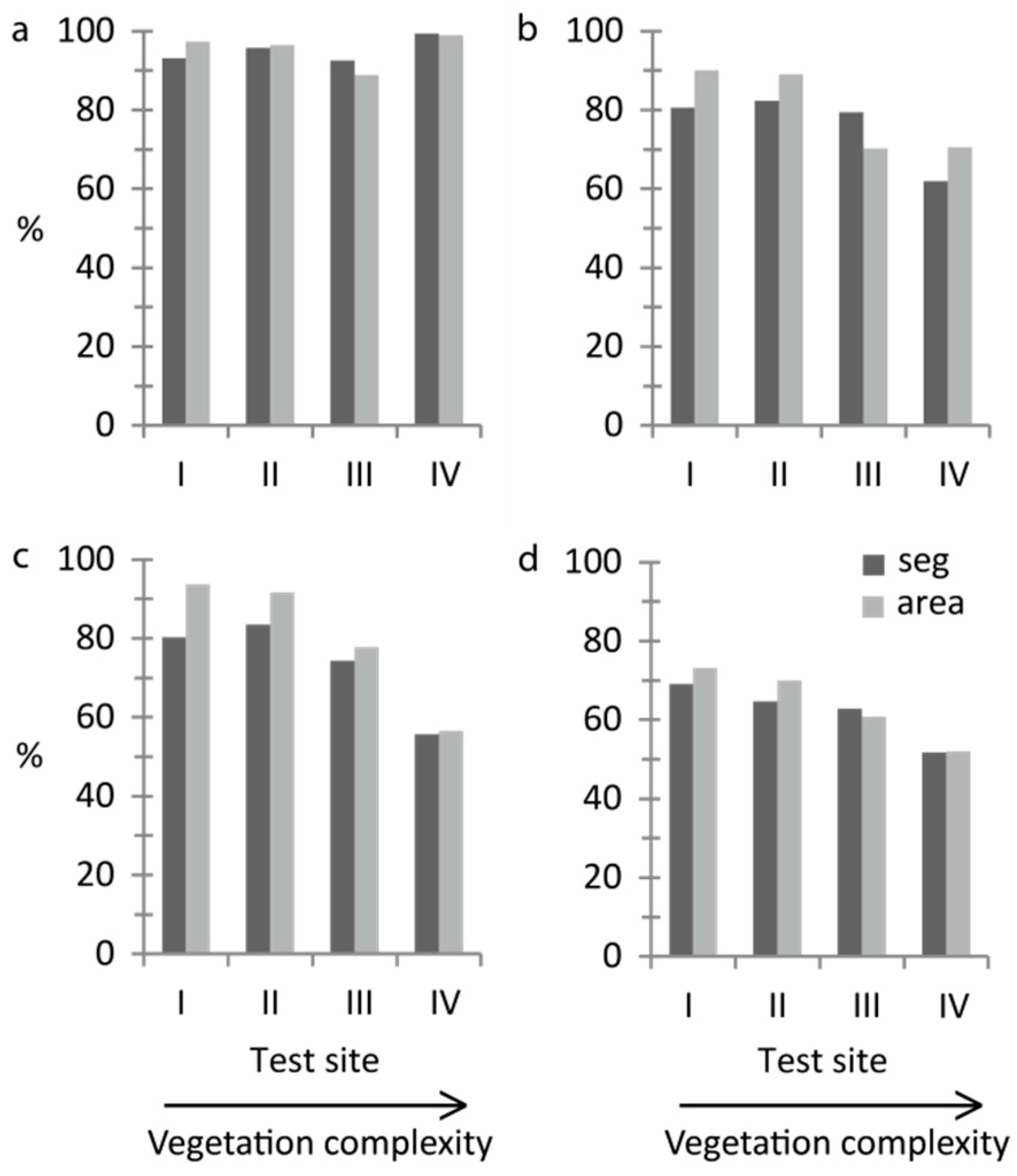
The quick and straightforward threshold method successfully separated water and vegetation. More than 90% of the validation segments were correctly classified at all sites and at least 89% of the area was correctly mapped (Figure 3a). Kappa coefficients ranged from 0.60–0.83 (Table S1). At the majority of sites quantity disagreement was larger than allocation disagreement (Table S1). In all cases, vegetation had a higher Producer’s accuracy than water (Table 5). Differences in User’s accuracy were less pronounced. The error matrices for all levels of detail at all sites are included in Table S1. We found the texture feature “GLCM Homogeneity” to be best in distinguishing between water and vegetation at sites I–IV. In addition, the feature “Brightness” was used at site II and the feature “NDI Green–Blue” was used at site IV to optimise the classification. At site V, wave action had changed the characteristic texture of water, and in this case only “NDI Green–Blue” was used.
For growth form, overall accuracy decreased with increasing vegetation complexity (Figure 3b,c). With the threshold method, the correctly classified area was at least 70% at all sites (Figure 3b). The percentage of correctly classified validation segments was lowest at site IV (62%) but was around 80% at sites I–III (Figure 3b). Kappa coefficients for the threshold classification ranged from 0.16–0.52 (Table S1). At the majority of sites quantity disagreement was larger than allocation disagreement (Table S1). The feature “Brightness” was used to separate helophytes and nymphaeids at all sites. In addition, the feature “Hue” was used at site IV and the feature “NDI Green–Red” was used at site V to optimise the threshold classification. The two tested classification methods gave similar results, except at the most complex site IV where the overall classification accuracy was 56% with Random Forest (Figure 3c). Kappa coefficients for the Random Forest classification ranged from 0.25–0.69 (Table S1). At the majority of sites allocation disagreement was larger than quantity disagreement (Table S1). Producer’s and User’s accuracies for growth form varied between classes and sites (Table 6).
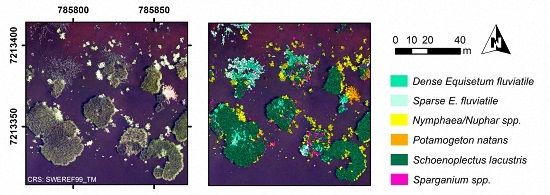
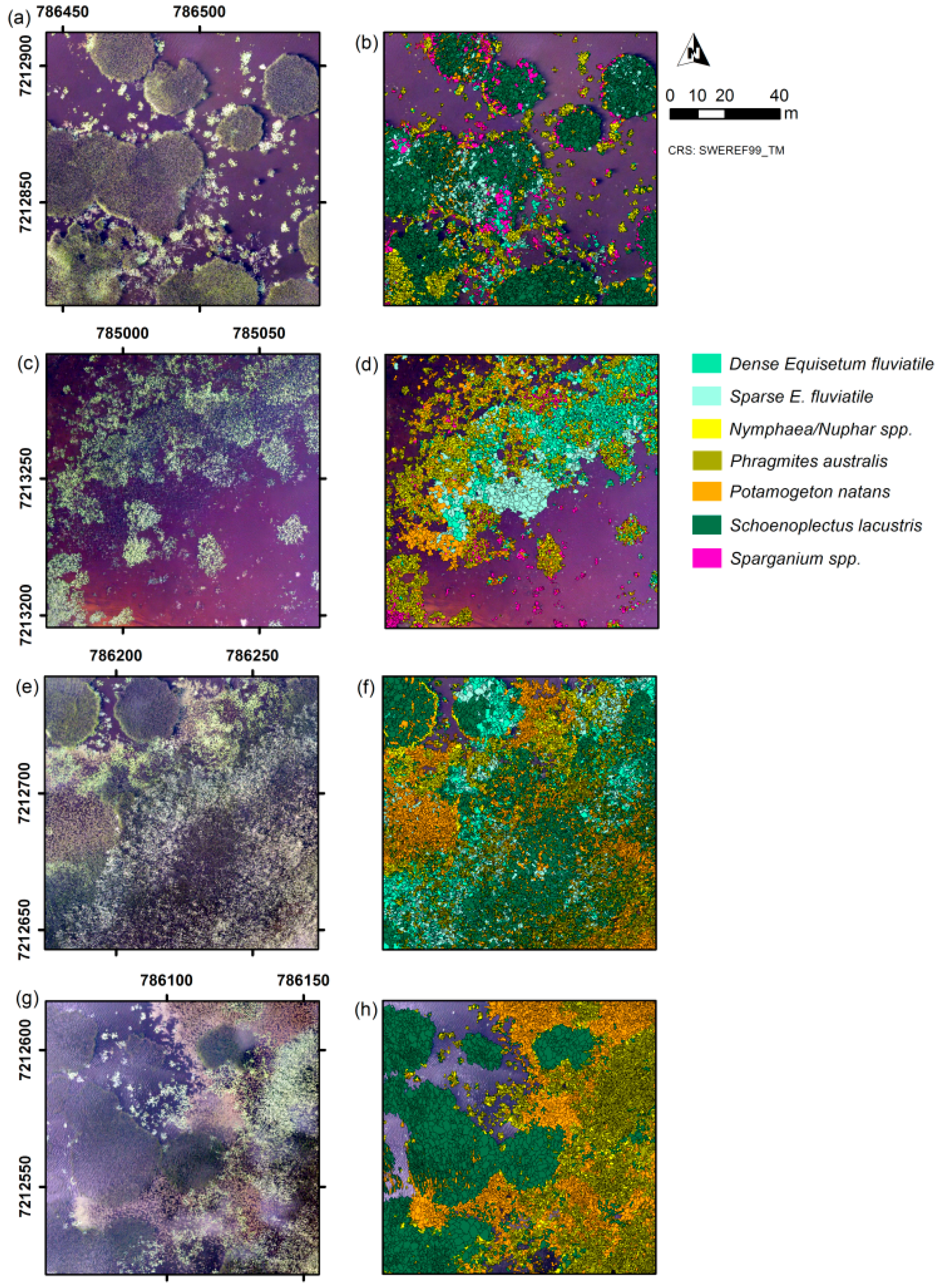
At the most advanced level of detail, dominant taxon (Figure 1h and Figure 2b,d,f,h), overall accuracies decreased with increasing vegetation complexity and 70% correctly classified area was reached only at sites I and II (Figure 3d). Kappa coefficients ranged from 0.34–0.54 (Table S1). At the majority of sites quantity disagreement was larger than allocation disagreement (Table S1). Producer’s and User’s accuracies showed large variation between classes and sites (Table 7). Nymphaea/Nuphar spp. was most reliably classified with User’s and Producer’s accuracies of at least 61% at all sites (segment-based, Table 7). Also S. lacustris had a minimum User’s and Producer’s accuracy of 65%, except for the Producer’s accuracy at site IV (43% segment-based and 51% area-based). The two E. fluviatile classes, P. natans and Sparganium spp. had in all cases a lower User’s than Producer’s accuracy indicating a large number of false inclusions (segment-based, Table 7). P. australis, which occurred at site IV–V, was confused with all other taxa present at site IV, but most frequently with the E. fluviatile classes and P. natans, resulting in a Producer’s accuracy of 48%.
Overall accuracies at site V were within the same range of overall accuracies at the other test sites for all performed OBIAs (Table S1), except for the area-based accuracy assessment for dominant-taxon (Figure 2h) where site V surprisingly showed the highest overall accuracy among all sites (75%). The segment-based overall accuracy was 65%.
The increase in accuracy (Inon-dom) owing to non-dominant-taxon classifications for segment-based and area-based accuracy assessment, respectively, was 0.3% and 0.1% at site I, 0.8% and 0.2% at site II, 8.4% and 6.2% at site III, 3.3%, and 3.4% at site IV, and 4.6% and 3.5% at site V. The increase was most pronounced at sites III–V which had a high proportion of mixed vegetation stands (Table 2). Including non-dominant-taxon classifications, site III showed the highest segment-based accuracy of all sites (71%).
The manual mapping took 2.06 h at site I and 5.39 h at site IV. The automated dominant-taxon classification took 2.25 h at site I and 2.12 h at site IV.

4. Discussion

Our results demonstrate that it is feasible to extract ecologically relevant information on non-submerged aquatic vegetation from UAS-orthoimages in an automated way. The automatization increases time-efficiency compared to manual mapping, but might decrease classification accuracy with increased vegetation complexity. The classification accuracies achieved in our study lie in the range of accuracies reported from other OBIA studies in wetland environments as reviewed by Dronova [33]. The exception to this is for the growth-form and dominant-taxon level at the most complex site IV. Here, presence of P. australis increased the number of misclassifications on the dominant-taxon level and the growth-form level, where P. australis was to a large extent classified as nymphaeid, probably due to its light green colour. Site IV also has the highest number of mixed-vegetation classes in the manual mapping, but non-dominant-taxon classifications were only of minor importance in explaining misclassifications. The two taxa that were most reliably classified regarding all sites, Nymphaea/Nuphar spp. and S. lacustris, typically covered large areas. High within-taxon variation of S. lacustris (as also observed by Husson et al. [16]) posed problems for the automated classification. Bent stems with high sun exposure, typically at the edge of vegetation stands, as well as straight stems with low area coverage were repeatedly misclassified. Because these areas were small in comparison to the total area of S. lacustris, accuracies for this taxon were not highly affected. However, these misclassifications had a major impact on the classification accuracy of taxa with smaller total areas (E. fluviatile, P. natans, and Sparganium spp.) by increasing the number of false inclusions, giving low User’s accuracies.
At four out of five test sites, OBIA combined with Random Forest proved to be an appropriate automated classification method, in most cases giving good classification accuracies at a high level of detail (i.e., >75% for growth forms and >60% for dominant taxa). One way to raise classification accuracy (even at site IV) could be to manually choose training samples of high quality. The inclusion of segments with mixed vegetation as training samples due to random selection might have influenced the result because Random Forest is sensitive to inaccurate training data [39]. The threshold method is more intuitive compared to Random Forest and can be quick when expert-knowledge for feature selection is available. No samples and no ruleset are needed, which makes thresholding easier to use. A drawback of the threshold method is the limited number of classes. In contrast to Random Forest, two thresholding steps were necessary to get to the growth-form level. For more complex classification tasks, empirical determination of thresholds is not time-efficient. Empirical determination also increases subjectivity and limits the transferability of classification settings to other sites. A more automated approach to determine thresholds should be evaluated in the future.
The results for site V indicate that the method used here could cope with poor image quality. The surprisingly high overall classification accuracy at the dominant-taxon level at site V was probably caused by a favourable species composition that reduced the risk for confusion between taxa. There was a large difference between segment-based and area-based accuracy assessment, likely because some of the correctly classified segments at site V covered a large area.
A challenge in OBIA is the relative flexibility in the framework (e.g., [33]). Segmentation parameters, classification method, and discriminating object features influence the classification result; routines for an objective determination of these parameters are still missing. We used a relatively small scale parameter, resulting in segments that were smaller than the objects (i.e., vegetation stands) to be classified (over-segmentation). This is advantageous in comparison to under-segmentation [51], because if one segment contains more than one object, a correct classification is impossible. Kim et al. [44] and Ma et al. [52] found that the optimal segmentation scale varied between classes; by using multiple segmentation scales, classification results could be optimised.
Time-measurement revealed that manual mapping of dominant taxa can be faster than OBIA in cases where vegetation cover and complexity level is low. However, regarding time-efficiency in general and for areas larger than our 100 m × 100 m test sites, automated classification out-performs manual mapping. This is because manual-mapping time is proportional to the mapped area, i.e., if the area doubles so does the time needed for manual mapping. A doubling of the area would, however, have only a small effect on the time needed to execute the OBIA, mainly through an increase in processing time and potentially an increase in the time needed for the assembly of reference data over a larger area. However, when applying OBIA to large or multiple image files, there may be limitations due to restrictions in computing power.
Heavy rains after the image acquisition forced us to postpone the field work to the next growing season. The one-year time lag between image acquisition and field work is a potential source of error. However, during field work the aquatic plants were in the same development stage as during image acquisition and the vegetation appeared very similar to the printed images. We were able to locate both training and control points selected on the UAS-orthoimage in 2011 in the field in 2012 without problems. This is confirmed by the high number of correct predictions during the image interpreter training. Another potential source of error relates to misclassifications of taxa during manual mapping which might have caused incorrect training and validation data. In a comparable lake environment but with a larger variety of taxa, Husson et al. [16] achieved an overall accuracy of 95% for visual identification of species.
Lightweight UASs are flexible and easy to handle allowing their use even in remote areas which are difficult to access for field work. UAS-technology is also especially favourable for monitoring purposes with short and/or user-defined repetition intervals. Our automated classification approach for water versus vegetation and at the growth-form level is highly applicable in lake and river management [53] and aquatic plant control, such as in evaluation of rehabilitation measures [54]. Valta-Hulkkonen et al. [55] also found that a lake’s degree of colonisation by helophytes and nymphaeids detected by remote sensing was positively correlated with the nutrient content in the water. For a full assessment of ecological status of lakes, it is, at the moment, not possible to replace field sampling by the method proposed here, partly due to uncertainty in the classification of certain taxa (which might be solved in the future) but also because submerged vegetation is not included. The latter is a considerably larger problem in temperate regions, where hydrophyte flora dominates, than in the boreal region where the aquatic flora naturally has a high proportion of emergent plants [18]. In the boreal region with its high number of lakes, the proposed method has large potential. Most boreal region lakes are humic [56] with high colour content which increases the importance of non-submerged plants because low water transparency hinders the development of submerged vegetation [57]. The taxonomical resolution achieved in our classification allows calculation of a remote-sensing-based ecological assessment index for non-submerged vegetation in coloured lakes, as suggested by Birk and Ecke [20].
UASs are still an emerging technology facing technical and regulatory challenges [58]. In the future, a systematic approach to explore image quality problems associated with UAS-imagery is needed. Compared to conventional aerial imagery, the close-to-nadir perspective in the UAS-orthoimage reduced angular variation and associated relief displacement of the vegetation. We used high image overlap and external ground control points for georeferencing. Therefore, the geometric accuracy and quality of the produced orthoimage in our study was not affected by autopilot GPS accuracy or aircraft stability (see also [16]). However, of concern for image quality was that the UAS-orthoimage was assembled from different flights undertaken at different times of the day and under varying weather conditions. This resulted in different degrees of wave action, cloud reflection, and sunglint, as well as varying position and size of shadows in different parts of the orthoimage. The high image overlap allowed for exclusion of individual images with bad quality from the data set prior to orthoimage production. In Sweden, UASs that may be operated by registered pilots without special authorisation at heights above 120 m can have a maximum total weight of 1.5 kg [59]. A challenge with those miniature UASs is limited payload [15]. Therefore, we used a lightweight digital compact camera. Here, very-high-resolution true-colour images performed well, without compromising UAS flexibility. However, due to recent technical development and progress in miniaturisation of sensors, lightweight UAS with multispectral and hyperspectral sensors are becoming available (e.g., [60]), even if such equipment still is relatively expensive. Inclusion of more optical bands (especially in the (near-)infrared region [39]) in UAS-imagery will likely increase classification accuracy at a high taxonomic level. Another relevant development is deriving 3D data from stereo images or UAS LiDAR sensors, enabling inclusion of height data together with spectral data, potentially improving the accuracy of automated growth-form and taxon discrimination [61].

5. Conclusions

True-colour images taken by UASs with sub-decimetre spatial resolution will be increasingly available for ecological applications in the future. We demonstrated that ecologically relevant information on non-submerged aquatic vegetation can be automatically extracted from these images. The classification of water versus vegetation, growth form, and certain taxa was feasible at test sites with varying vegetation complexity and image quality using object-based image analysis (OBIA) on a UAS-orthoimage with 5-cm pixel resolution. At sites of more complex vegetation, OBIA in combination with the Random Forest classification was more time-efficient than manual mapping. When choosing the preferred mapping method (manual versus automated) the desired level of thematic detail and required accuracy for the mapping task needs to be considered. When information on a high taxonomic level is crucial and the area to cover is not too large, manual mapping is superior to automated classification in terms of accuracy and resolution of information (e.g., possibility to map non-dominant taxa, see also [16]). However, when the focus is on covering larger areas, OBIA offers a more efficient alternative.

Supplementary Materials

The following are available online at www.mdpi.com/2072-4292/8/9/724/s1, Figure S1: Classification scheme for the manual mapping, Table S1: Error matrices for all sites at all levels of detail.

Acknowledgments

We thank Fredrik Lindgren for help with field work and Olle Hagner for help with the aerial survey. This work was funded by the Swedish Research Council Formas (reference number 2014-1425), and conducted as part of the European project ImpactMin (project number 244166 in FP7-ENV-2009-1) as well as the research programme WATERS, funded by the Swedish Environmental Protection Agency (Dnr 10/179) and Swedish Agency for Marine and Water Management.

Author Contributions

All authors conceived and designed the study; Eva Husson performed the field work and analysed the image data; Eva Husson wrote the paper with contributions of Frauke Ecke and Heather Reese.

Conflicts of Interest

The authors declare no conflict of interest.

Abbreviations

The following abbreviations are used in this manuscript:
LiDARLight detection and ranging
NDINormalised difference index
GLCMGrey-level co-occurrence matrix
GLCVGrey-level difference vector
GPSGlobal positioning system
OBIAObject-based image analysis
PAMSPersonal Aerial Mapping System
RGBRed green blue
UASUnmanned aircraft system

References

  1. Strayer, D. Ecology of freshwater shore zones. Aquat. Sci. 2010, 72, 127–163. [Google Scholar] [CrossRef]
  2. Pieczynska, E. Detritus and nutrient dynamics in the shore zone of lakes—A review. Hydrobiologia 1993, 251, 49–58. [Google Scholar] [CrossRef]
  3. Smith, C.S.; Adams, M.S. Phosphorus Transfer from Sediments by Myriophyllum-Spicatum. Limnol. Oceanogr. 1986, 31, 1312–1321. [Google Scholar] [CrossRef]
  4. Moller, C.L.; Sand-Jensen, K. Rapid oxygen exchange across the leaves of Littorella uniflora provides tolerance to sediment anoxia. Freshw. Biol. 2012, 57, 1875–1883. [Google Scholar] [CrossRef]
  5. Wetzel, R. Limnology, 3rd ed.; Elsevier: San Diego, CA, USA, 2001; p. 1006. [Google Scholar]
  6. EU. Directive 2000/60/ec of the European parliament and of the council of 23 October 2000 establishing a framework for community action in the field of water policy (rule number L 327). In Official Journal of the European Communities; EU (European Union): Brussels, Belgium, 2000; Volume 43. [Google Scholar]
  7. EPA. Lake and Reservoir Bioassessment and Biocriteria: Technical Guidance Document; United States Environmental Protection Agency: Washington, DC, USA, 1998.
  8. Hart, B.T.; Cambell, I.C.; Angehrn-Bettinazzi, C.; Jones, M.J. Australian water quality guidelines: A new approach for protecting ecosystem health. J. Aquat. Ecosyst. Stress Recov. 1993, 2, 151–163. [Google Scholar] [CrossRef]
  9. Markovic, D.; Carrizo, S.; Freyhof, J.; Cid, N.; Lengyel, S.; Scholz, M.; Kasperdius, H.; Darwall, W. Europe’s freshwater biodiversity under climate change: Distribution shifts and conservation needs. Divers. Distrib. 2014, 20, 1097–1107. [Google Scholar] [CrossRef]
  10. Davis, J.; O’Grady, A.P.; Dale, A.; Arthington, A.H.; Gell, P.A.; Driver, P.D.; Bond, N.; Casanova, M.; Finlayson, M.; Watts, R.J.; et al. When trends intersect: The challenge of protecting freshwater ecosystems under multiple land use and hydrological intensification scenarios. Sci. Total Environ. 2015, 534, 65–78. [Google Scholar] [CrossRef] [PubMed]
  11. Vitousek, P.M.; Dantonio, C.M.; Loope, L.L.; Rejmanek, M.; Westbrooks, R. Introduced species: A significant component of human-caused global change. N. Z. J. Ecol. 1997, 21, 1–16. [Google Scholar]
  12. Silva, T.S.F.; Costa, M.P.F.; Melack, J.M.; Novo, E. Remote sensing of aquatic vegetation: Theory and applications. Environ. Monit. Assess. 2008, 140, 131–145. [Google Scholar] [CrossRef] [PubMed]
  13. Miler, O.; Ostendorp, W.; Brauns, M.; Porst, G.; Pusch, M.T. Ecological assessment of morphological shore degradation at whole lake level aided by aerial photo analysis. Fundam. Appl. Limnol. 2015, 186, 353–369. [Google Scholar] [CrossRef]
  14. Husson, E.; Lindgren, F.; Ecke, F. Assessing biomass and metal contents in riparian vegetation along a pollution gradient using an unmanned aircraft system. Water Air Soil Pollut. 2014, 225. [Google Scholar] [CrossRef]
  15. Anderson, K.; Gaston, K.J. Lightweight unmanned aerial vehicles will revolutionize spatial ecology. Front. Ecol. Environ. 2013, 11, 138–146. [Google Scholar] [CrossRef]
  16. Husson, E.; Hagner, O.; Ecke, F. Unmanned aircraft systems help to map aquatic vegetation. Appl. Veg. Sci. 2014, 17, 567–577. [Google Scholar] [CrossRef]
  17. Penning, W.E.; Mjelde, M.; Dudley, B.; Hellsten, S.; Hanganu, J.; Kolada, A.; van den Berg, M.; Poikane, S.; Phillips, G.; Willby, N.; et al. Classifying aquatic macrophytes as indicators of eutrophication in European lakes. Aquat. Ecol. 2008, 42, 237–251. [Google Scholar] [CrossRef]
  18. Alahuhta, J.; Kanninen, A.; Hellsten, S.; Vuori, K.M.; Kuoppala, M.; Hamalainen, H. Variable response of functional macrophyte groups to lake characteristics, land use, and space: Implications for bioassessment. Hydrobiologia 2014, 737, 201–214. [Google Scholar] [CrossRef]
  19. Alahuhta, J.; Kanninen, A.; Vuori, K.-M. Response of macrophyte communities and status metrics to natural gradients and land use in boreal lakes. Aquat. Bot. 2012, 103, 106–114. [Google Scholar] [CrossRef]
  20. Birk, S.; Ecke, F. The potential of remote sensing in ecological status assessment of coloured lakes using aquatic plants. Ecol. Indic. 2014, 46, 398–406. [Google Scholar] [CrossRef]
  21. CEN. Water Quality—Guidance Standard for the Surveying of Macrophytes in Lakes; Standard Number EN 15460:2007; CEN (European Committee for Standardisation): Brussels, Belgium, 2007. [Google Scholar]
  22. EPA. 2012 National Lakes Assessment: Field Operations Manual; United States Environmental Protection Agency: Washington, DC, USA, 2012.
  23. Björk, S. The evolution of lakes and wetlands. In Restoration of Lakes, Streams, Floodplains, and Bogs in Europe: Principles and Case Studies; Eiseltova, M., Ed.; Springer: Dordrecht, The Netherlands, 2010; Volume 3, pp. 25–35. [Google Scholar]
  24. Walker, P.D.; Wijnhoven, S.; van der Velde, G. Macrophyte presence and growth form influence macroinvertebrate community structure. Aquat. Bot. 2013, 104, 80–87. [Google Scholar] [CrossRef]
  25. Kuczynska-Kippen, N.; Wisniewska, M. Environmental predictors of rotifer community structure in two types of small water bodies. Int. Rev. Hydrobiol. 2011, 96, 397–404. [Google Scholar] [CrossRef]
  26. Holopainen, S.; Arzel, C.; Dessborn, L.; Elmberg, J.; Gunnarsson, G.; Nummi, P.; Poysa, H.; Sjoberg, K. Habitat use in ducks breeding in boreal freshwater wetlands: A review. Eur. J. Wildl. Res. 2015, 61, 339–363. [Google Scholar] [CrossRef]
  27. Ecke, F.; Henry, A.; Danell, K. Landscape-based prediction of the occurrence of the invasive muskrat (Ondatra zibethicus). Ann. Zool. Fenn. 2014, 51, 325–334. [Google Scholar] [CrossRef]
  28. Laliberte, A.S.; Herrick, J.E.; Rango, A.; Winters, C. Acquisition, orthorectification, and object-based classification of unmanned aerial vehicle (UAV) imagery for rangeland monitoring. Photogramm. Eng. Remote Sens. 2010, 76, 661–672. [Google Scholar] [CrossRef]
  29. Halabisky, M.; Moskal, L.M.; Hall, S.A. Object-based classification of semi-arid wetlands. J. Appl. Remote Sens. 2011, 5. [Google Scholar] [CrossRef]
  30. Blaschke, T.; Hay, G.J.; Kelly, M.; Lang, S.; Hofmann, P.; Addink, E.; Feitosa, R.Q.; van der Meer, F.; van der Werff, H.; van Coillie, F.; et al. Geographic object-based image analysis—Towards a new paradigm. ISPRS J. Photogramm. Remote Sens. 2014, 87, 180–191. [Google Scholar] [CrossRef] [PubMed]
  31. Laliberte, A.S.; Rango, A. Texture and scale in object-based analysis of subdecimeter resolution unmanned aerial vehicle (UAV) imagery. IEEE Trans. Geosci. Remote Sens. 2009, 47, 761–770. [Google Scholar] [CrossRef]
  32. Yu, Q.; Gong, P.; Clinton, N.; Biging, G.; Kelly, M.; Schirokauer, D. Object-based detailed vegetation classification with airborne high spatial resolution remote sensing imagery. Photogramm. Eng. Remote Sens. 2006, 72, 799–811. [Google Scholar] [CrossRef]
  33. Dronova, I. Object-based image analysis in wetland research: A review. Remote Sens. 2015, 7, 6380–6413. [Google Scholar] [CrossRef]
  34. Breiman, L. Random forests. Mach. Learn. 2001, 45, 5–32. [Google Scholar] [CrossRef]
  35. Sjörs, H. The background: Geology, climate and zonation. In Swedish Plant Geography; Rydin, H., Snoeijs, P., Diekmann, M., Eds.; Svenska Växtgeografiska Sällskapet: Uppsala, Sweden, 1999; pp. 5–14. [Google Scholar]
  36. VISS—Water Information System Sweden. Available online: http://www.viss.lansstyrelsen.se/Waters.aspx?waterEUID=SE721083-174843 (accessed on 4 April 2016).
  37. Baatz, M.; Schäpe, A. Multiresolution segmentation—An optimization approach for high quality multi-scale image segmentation. In Angewandte Geographische Informationsverarbeitung XII; Strobl, J., Ed.; Wichmann: Heidelberg, Germany, 2000; pp. 12–23. [Google Scholar]
  38. Congalton, R.G.; Green, K. Assessing the Accuracy of Remotely Sensed Data: Principles and Practices, 2nd ed.; CRC Press: Boca Raton, FL, USA, 2009; p. 192. [Google Scholar]
  39. Lang, M.W.; Bourgeau-Chavez, L.L.; Tiner, R.W.; Klemas, V.V. Chapter 5: Advances in remotely sensed data and techniques for wetland mapping and monitoring. In Remote Sensing of Wetlands: Applications and Advances; Tiner, R.W., Lang, M.W., Klemas, V.V., Eds.; CRC Press: Boca Raton, FL, USA, 2015. [Google Scholar]
  40. Rodriguez-Galiano, V.F.; Ghimire, B.; Rogan, J.; Chica-Olmo, M.; Rigol-Sanchez, J.P. An assessment of the effectiveness of a random forest classifier for land-cover classification. ISPRS J. Photogramm. Remote Sens. 2012, 67, 93–104. [Google Scholar] [CrossRef]
  41. Stefanski, J.; Mack, B.; Waske, B. Optimization of object-based image analysis with random forests for land cover mapping. IEEE J. Sel. Top. Appl. Earth Obs. Remote Sens. 2013, 6, 2492–2504. [Google Scholar] [CrossRef]
  42. Haralick, R.M.; Shanmugam, K.; Dinstein, I.H. Textural features for image classification. IEEE Trans. Syst. Man Cybern. 1973, 3, 610–621. [Google Scholar] [CrossRef]
  43. Laliberte, A.; Rango, A. Incorporation of texture, intensity, hue, and saturation for rangeland monitoring with unmanned aircraft imagery. In Proceedings of the GEOBIA 2008, Calgary, AB, Canada, 5–8 August 2008.
  44. Kim, M.; Warner, T.A.; Madden, M.; Atkinson, D.S. Multi-scale GEOBIA with very high spatial resolution digital aerial imagery: Scale, texture and image objects. Int. J. Remote Sens. 2011, 32, 2825–2850. [Google Scholar] [CrossRef]
  45. Laliberte, A.S.; Rango, A. Image processing and classification procedures for analysis of sub-decimeter imagery acquired with an unmanned aircraft over arid rangelands. Giscience Remote Sens. 2011, 48, 4–23. [Google Scholar] [CrossRef]
  46. Hunt, E.R.; Cavigelli, M.; Daughtry, C.S.T.; McMurtrey, J.; Walthall, C.L. Evaluation of digital photography from model aircraft for remote sensing of crop biomass and nitrogen status. Precis. Agric. 2005, 6, 359–378. [Google Scholar] [CrossRef]
  47. Radoux, J.; Bogaert, P.; Fasbender, D.; Defourny, P. Thematic accuracy assessment of geographic object-based image classification. Int. J. Geogr. Inf. Sci. 2011, 25, 895–911. [Google Scholar] [CrossRef]
  48. Congalton, R.G. A review of assessing the accuracy of classifications of remotely sensed data. Remote Sens. Environ. 1991, 37, 35–46. [Google Scholar] [CrossRef]
  49. Pontius, R.G.; Millones, M. Death to kappa: Birth of quantity disagreement and allocation disagreement for accuracy assessment. Int. J. Remote Sens. 2011, 32, 4407–4429. [Google Scholar] [CrossRef]
  50. Woodcock, C.E.; Gopal, S. Fuzzy set theory and thematic maps: Accuracy assessment and area estimation. Int. J. Geogr. Inf. Sci. 2000, 14, 153–172. [Google Scholar] [CrossRef]
  51. Liu, D.S.; Xia, F. Assessing object-based classification: Advantages and limitations. Remote Sens. Lett. 2010, 1, 187–194. [Google Scholar] [CrossRef]
  52. Ma, L.; Cheng, L.; Li, M.C.; Liu, Y.X.; Ma, X.X. Training set size, scale, and features in geographic object-based image analysis of very high resolution unmanned aerial vehicle imagery. ISPRS J. Photogramm. Remote Sens. 2015, 102, 14–27. [Google Scholar] [CrossRef]
  53. Casado, M.R.; Gonzalez, R.B.; Kriechbaumer, T.; Veal, A. Automated identification of river hydromorphological features using UAV high resolution aerial imagery. Sensors 2015, 15, 27969–27989. [Google Scholar] [CrossRef] [PubMed] [Green Version]
  54. Valta-Hulkkonen, K.; Kanninen, A.; Pellikka, P. Remote sensing and GIS for detecting changes in the aquatic vegetation of a rehabilitated lake. Int. J. Remote Sens. 2004, 25, 5745–5758. [Google Scholar] [CrossRef]
  55. Valta-Hulkkonen, K.; Kanninen, A.; Iivonen, R.; Leka, J. Assessment of aerial photography as a method for monitoring aquatic vegetation in lakes of varying trophic status. Boreal Environ. Res. 2005, 10, 57–66. [Google Scholar]
  56. Likens, G. Lake Ecosystem Ecology: A Global Perspective; Acadenic Press: San Diego, CA, USA, 2010; p. 480. [Google Scholar]
  57. Sondergaard, M.; Phillips, G.; Hellsten, S.; Kolada, A.; Ecke, F.; Maeemets, H.; Mjelde, M.; Azzella, M.M.; Oggioni, A. Maximum growing depth of submerged macrophytes in European lakes. Hydrobiologia 2013, 704, 165–177. [Google Scholar] [CrossRef]
  58. Zweig, C.L.; Burgess, M.A.; Percival, H.F.; Kitchens, W.M. Use of unmanned aircraft systems to delineate fine-scale wetland vegetation communities. Wetlands 2015, 35, 303–309. [Google Scholar] [CrossRef]
  59. Transportstyrelsen. Transportstyrelsens Föreskrifter om Verksamhet med Obemannade Luftfartyg (UAS); Regulation Number TSFS 2009:88; Transportstyrelsen (Swedish Transport Agency): Norrköping, Sweden, 2009. [Google Scholar]
  60. SmartPlanes. Available online: http://smartplanes.se/launch-of-new-products/ (accessed on 14 April 2016).
  61. Madden, M.; Jordan, T.; Bernardes, S.; Cotten, D.L.; O’Hare, N.; Pasqua, A. Unmanned aerial systems and structure from motion revolutionize wetlands mapping. In Wetlands: Applications and Advances; Tiner, R.W., Lang, M.W., Klemas, V.V., Eds.; CRC Press: Boca Raton, FL, USA, 2015; pp. 195–219. [Google Scholar]
Figure 1. Location of the test sites within Lake Ostträsket (a) and exemplification using test site I: Orthoimage (b); Manual mapping (c); Reference Map (d); Water-versus-vegetation classification using thresholding (e); Growth-form classification using thresholding (f); Growth-form classification using Random Forest (g); Dominant-taxon classification using Random Forest (h).
Remotesensing 08 00724 g001
Figure 2. Orthoimage of test sites II (a); III (c); IV (e); and V (g) and corresponding dominant-taxon classification using Random Forest at test sites II (b); III (d); IV (f); and V (h).
Remotesensing 08 00724 g002
Figure 3. Overall accuracy for sites I–IV for (a) water-versus-vegetation classification using thresholding; (b) growth-form classification using thresholding; (c) growth-form classification using Random Forest; and (d) dominant-taxon classification using Random Forest. Seg: assessment based on number of validation segments, area: assessment based on area of validation segments.
Remotesensing 08 00724 g003
Table 1. Species inventory list of non-submerged vegetation at Lake Ostträsket with number of observations (NO) within 25 circle plots, radius 10 m.
SpeciesNO
Helophytes
Equisetum fluviatile13
Schoenoplectus lacustris13
Phragmites australis3
Carex rostrata1
Nymphaeids
Nuphar lutea18
Potamogeton natans15
Sparganium spp.7
Nymphaea alba ssp. candida4
Nuphar pumila2
Table 2. Test site description including vegetation classes as derived from the manual mapping; dense Equisetum fluviatile (ef_d), sparse E. fluviatile (ef_s), Nymphaea/Nuphar spp. (ny), Phragmites australis (pa), Potamogeton natans (pn), Schoenoplectus lacustris (sl), and Sparganium spp. (sp).
SiteTaxaVegetation Classes (in Order of Decreasing Area)Vegetated Area (%)Mixed Vegetation (% of Vegetated Area)
Ief, ny, pn, sl, spwater, sl, ny, ef_d, ef_s, pn, sp, ef_d & sl, sl & ef, sl & ny, ny & sl, ny & ef362
IIef, ny, pn, sl, spsl, water, ny, sp, pn, ef_d, ef_s, ny & sl, pn & ef, ny & ef, sl & ny, ny & pn, pn & ny, sl & pn614
IIIef, ny, pn, spwater, ny, ef_s, ny & ef, ef_d, ny & pn, pn, ef_d & ny, sp, ef_s & ny, pn & ef, sp & ny, pn & ny, ny & sp5526
IVef, ny, pa, pn, slsl, pa, pa & sl, pn, ny, sl & pa, water, sl & ny, ny & pn, ef_d, pn & sl, ny & sl, ef_s, ny & ef, ef_d & sl, pn & ny, pa & ny, ef_d & ny, sl & pn, ef_s & ny & pn9626
Vny, pa, pn, slsl, pn, pa, water, ny & pn, ny, pn & sl, sl & pn, sl & pa, pa & sl, sl & ny, pn & ny, pa & pn, pa & ny, pa & pn & ny, ny & sl, pn & pa8621
Table 3. Object-based image analyses (OBIAs) performed on each individual test site. Class names have been abbreviated as follows: dense Equisetum fluviatile (ef_d), sparse E. fluviatile (ef_s), Nymphaea/Nuphar spp. (ny), Phragmites australis (pa), Potamogeton natans (pn), Schoenoplectus lacustris (sl), and Sparganium spp. (sp).
OBIALevel of DetailClassesClassification MethodApplied to
(a)water versus vegetationwater, vegetationthresholdentire test site
(b)growth formnymphaeid, helophytethresholdvegetated area
(c)growth formwater, nymphaeid, helophyteRandom Forestentire test site
(d)dominant taxonef_d, ef_s, ny, pa, pn, sl, spRandom Forestvegetated area
Table 4. Object features used in the Random Forest classification.
Spectral Features “HSI Transformation” 1“Texture after Haralick” 1,2Normalised Difference Index
 Individual for each band: • Hue derived from GLCM: derived from GLCV: • NDI Green–Blue
 • Mean • Saturation • Ang. 2nd moment • Ang. 2nd moment • NDI Green–Red
 • Mode (median) • Intensity • Contrast • Contrast • NDI Red−Blue
 • Quantile (50%)  • Correlation • Entropy
 • Standard deviation  • Dissimilarity • Mean
 • Ratio  • Entropy
 • Max. pixel value  • Homogeneity
 For all bands combined:  • Mean
 • Brightness  • Standard deviation
 • Max. difference
1 as termed in eCognition®; 2 mean of all bands, all directions; Ang.: Angular, GLCM: Grey-level co-occurrence matrix, GLCV: Grey-level difference vector.
Table 5. Producer’s and User’s accuracy (%) of water (W) versus vegetation (V) using a threshold classification.
Site ISite IISite IIISite IV
WVWVWVWV
Segment-based
No. of validation segments106244592915329710343
Producer’s accuracy799975100669750100
User’s accuracy989210095819410099
Area-based
Total area of validation segments (m2)44321216721115218914241
Producer’s accuracy979992100918859100
User’s accuracy999310094859210099
Table 6. Producer’s and User’s accuracy (%) of the growth forms nymphaeid (N) and helophyte (H) using a threshold classification and of water (W), nymphaeid, and helophyte using Random Forest.
Site ISite IISite IIISite IV
WNHWNHWNHWNH
Threshold classification: Segment-based
No. of validation segments 102248 108242 28763 74276
Producer’s accuracy 3798 4599 9033 5963
User’s accuracy 9079 9480 8641 3085
Threshold classification: Area-based
Total area of validation segments (m2) 59247 49210 14484 44202
Producer’s accuracy 5299 44100 8152 5674
User’s accuracy 9390 9788 7461 3288
Random Forest: Segment-based
No. of validation segments10668176578720652246521071274
Producer’s accuracy818279895992637869908249
User’s accuracy975884898482859235253392
Random Forest: Area-based
Total area of validation segments (m2)4583717716239176145121661842201
Producer’s accuracy978387965496897068927749
User’s accuracy995989978988879249353092
Table 7. Producer’s and User’s accuracy (%) of dominant taxa using Random Forest classification, number of validation segments (N) and total area of validation segments (A).
Segment-BasedArea-Based
NProducer’s AccuracyUser’s AccuracyA (m2)Producer’s AccuracyUser’s Accuracy
Site I
Sparse Equisetum fluviatile156041127633
Dense Equisetum fluviatile274833244133
Nymphaea/Nuphar spp.957978508371
Potamogeton natans108047109166
Schoenoplectus lacustris20668922147495
Sparganium spp.1040115318
Site II
Sparse Equisetum fluviatile10501276315
Dense Equisetum fluviatile10702945918
Nymphaea/Nuphar spp.907084407181
Potamogeton natans102064133
Schoenoplectus lacustris23065922057296
Sparganium spp.10702757223
Site III
Sparse Equisetum fluviatile404844616275
Dense Equisetum fluviatile225924227132
Nymphaea/Nuphar spp.27366941315795
Potamogeton natans125013117220
Sparganium spp.10703276738
Site IV
Sparse Equisetum fluviatile10801799219
Dense Equisetum fluviatile10409122311
Nymphaea/Nuphar spp.416168225670
Phragmites australis1704881954383
Potamogeton natans338838228934
Schoenoplectus lacustris1004369975177

