Article

Season Spotter: Using Citizen Science to Validate and Scale Plant Phenology from Near-Surface Remote Sensing

1
Department of Organismic and Evolutionary Biology, Harvard University, Cambridge, MA 02138, USA
2
National Ecological Observatory Network, Boulder, CO 80301, USA
*
Author to whom correspondence should be addressed.
Remote Sens. 2016, 8(9), 726; https://doi.org/10.3390/rs8090726
Submission received: 26 July 2016 / Revised: 18 August 2016 / Accepted: 23 August 2016 / Published: 1 September 2016
(This article belongs to the Special Issue Citizen Science and Earth Observation)

Abstract

:
The impact of a rapidly changing climate on the biosphere is an urgent area of research for mitigation policy and management. Plant phenology is a sensitive indicator of climate change and regulates the seasonality of carbon, water, and energy fluxes between the land surface and the climate system, making it an important tool for studying biosphere–atmosphere interactions. To monitor plant phenology at regional and continental scales, automated near-surface cameras are being increasingly used to supplement phenology data derived from satellite imagery and data from ground-based human observers. We used imagery from a network of phenology cameras in a citizen science project called Season Spotter to investigate whether information could be derived from these images beyond standard, color-based vegetation indices. We found that engaging citizen science volunteers resulted in useful science knowledge in three ways: first, volunteers were able to detect some, but not all, reproductive phenology events, connecting landscape-level measures with field-based measures. Second, volunteers successfully demarcated individual trees in landscape imagery, facilitating scaling of vegetation indices from organism to ecosystem. And third, volunteers’ data were used to validate phenology transition dates calculated from vegetation indices and to identify potential improvements to existing algorithms to enable better biological interpretation. As a result, the use of citizen science in combination with near-surface remote sensing of phenology can be used to link ground-based phenology observations to satellite sensor data for scaling and validation. Well-designed citizen science projects targeting improved data processing and validation of remote sensing imagery hold promise for providing the data needed to address grand challenges in environmental science and Earth observation.

Graphical Abstract

1. Introduction

Plant phenology, the timing of life history events such as leaf-out, flowering, seed-development, and senescence, is highly sensitive to weather, and is thus a key indicator of the impacts of climate change on Earth’s biota [1]. Warming spring temperatures over the past half century have caused plant species across the temperate zone to leaf out earlier [2,3]. Likewise, delayed autumn chilling has widely delayed leaf senescence [2,3,4], though the timing of spring phenology modifies this effect [5].
Currently, plant phenology is studied on the ground at the scale of the individual [6] or at broader scales using vegetation indices derived from satellite imagery [7] or near-surface automatic digital cameras [8]. Vegetation indices are typically used to track continuous photosynthetic activity of vegetation, whereas ground-based field measurements are often needed to determine discrete phenological events, including reproductive phenology [9,10]. Estimates of the effects of climate change on plant phenology using data at different scales vary [11], and so there is need to integrate phenology measures at different scales.
Midscale phenology cameras can provide a link between these different scales of observation by extracting information beyond vegetation indices from the camera imagery [10]. Because the spatial scale of these near-surface images is much finer than that of satellite imagery, details such as the presence or color of flowers, the foliation and color of individual tree canopies, and the occurrence of precipitation events (including rain, fog and snow) can be seen directly in camera images. Documenting the phenological state of individuals is typical of on-the-ground phenology data gathering efforts. However, phenology cameras have rarely been used to produce information beyond landscape-scale leaf canopy state (but see [12]).
Extracting these sorts of details—rather than general patterns of “vegetation greenness”—from phenology camera images requires sophisticated image analysis that has not yet been automated, and the sheer volume of imagery makes manual image analysis prohibitive for networks of more than a handful of cameras. Citizen science provides a solution for analyzing large image data sets to extract information that cannot yet be easily extracted by computational means [13]. Citizen scientist volunteers have successfully classified galaxy types from astronomical telescope images [14], found interstellar dust particles in electron microscope images [15], and identified animal species in camera trap images [16].
We created the citizen science project Season Spotter (seasonspotter.org) to analyze images from phenology cameras. Season Spotter uses images from the PhenoCam network, the largest near-surface phenology camera network in the world. It consists of 300 elevated cameras located primarily in North America and spans a wide range of ecosystem types (Figure 1) [8,17]. Automated processing of PhenoCam images produces a vegetation index (GCC, “green chromatic coordinate”) that indicates the relative amount of green in a predefined region of interest in each image [18]. This GCC index can then be used to infer the seasonal progression of leaf emergence and expansion, leaf color change, and senescence in the same manner as satellite-sensor-derived vegetation indices like NDVI and EVI [19]. GCC has also been shown to mirror the dynamics of carbon dioxide fluxes as measured by co-located eddy covariance instrumentation [20].
Season Spotter presented PhenoCam images from across a wide range of ecosystem types to volunteers using an online interface and asked the volunteers questions about these images. We algorithmically combined the volunteers’ answers into usable classifications. Season Spotter asked volunteers to: identify the reproductive and vegetative states of deciduous trees, evergreen trees, shrubs, grasses, forbs, and crops; identify poor quality images and those containing snow; outline individual trees at forested sites; and make phenological comparisons between two images taken at the same site.
Our goals for leveraging human visual perception using Season Spotter were threefold. First, we wanted to discern whether reproductive phenology (e.g., flowers, fruits, seeds) could be detected from these images to provide a complementary data product connecting landscape-level phenology measurements with field-based measures. Second, we wanted to see if individual trees could be identified and their vegetation indices calculated to facilitate scaling from local to regional scales. And third, we wanted to use citizen scientists’ assessments of spring and autumn start and end dates to evaluate dates calculated automatically from vegetation indices.

2. Materials and Methods

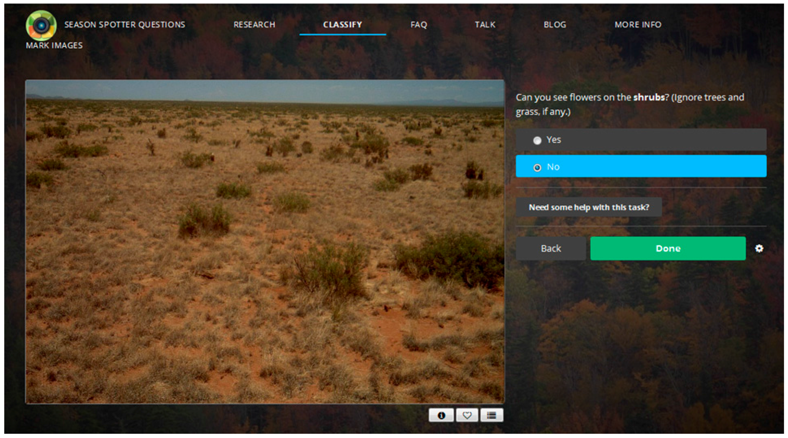
2.1. Citizen Science: Season Spotter

We created the online citizen science project Season Spotter (seasonspotter.org) using the Zooniverse Project Builder (www.zooniverse.org/lab) [21]. The Zooniverse is an online citizen science platform with 1.1 million current users, which hosts a variety of projects in need of volunteers to support data-processing tasks. The Season Spotter site consists of a landing page, which allows volunteers to choose whether they want to answer multiple-choice questions about PhenoCam images or demarcate specified regions on the images (Figure 2).
After making the choice, each volunteer begins one of multiple randomly assigned workflows (Figure 3 and Figure S1) that are tailored to the different ecosystem types. Each workflow consists of one or more tasks, including answering questions and drawing outlines. When a volunteer begins a workflow, a PhenoCam image is selected and presented to the volunteer along with its associated tasks. For each task, there is a help button that, when clicked, provides the volunteer with detailed instructions for the task to be completed together with example images. When the volunteer has finished answering questions and/or demarcating regions, the project shows a summary of the volunteer’s responses and a button to load a new image.
The summary also provides a button for entering a dedicated chat forum where volunteers can ask questions, comment on images, and interact with the Season Spotter science team and each other. Additional outreach and engagement is regularly conducted via the Season Spotter blog (seasonspotter.wordpress.com), Facebook (www.facebook.com/seasonspotter), and Twitter (twitter.com/seasonspotter).
In May 2015 we tested the Season Spotter project with a group of 39 volunteer beta testers. Using their feedback on a follow-up questionnaire, we modified task questions and added additional instructions and information to increase data quality. On 21 July 2015, we officially launched Season Spotter. The majority of volunteer recruitment occurred through Zooniverse email newsletters, though we undertook multiple recruitment activities [22].

2.2. PhenoCam Images

We uploaded 51,782 images to the Season Spotter project, divided into three groups. Each image came from a PhenoCam site (Table 1, Figure 4) and had its top or bottom cropped off to remove date information as well as to provide a more visually pleasing experience. The cropped images ranged from 640 × 452 pixels to 3888 × 2592 pixels, and image viewing resolution varied among volunteers by device, operating system, and browser.
The first group of 26,649 images (Group 1) was used to see if volunteers could extract information on reproductive and vegetation phenology, snow cover, and image quality from landscape images. Group 1 images were taken from the harvard and bartlettir sites, locations of previous and ongoing PhenoCam research [23,24], as well as PhenoCams at 14 other sites (Figure 4). We randomly selected these additional sites from a list of all PhenoCams that we judged to produce good-quality seasonal patterns in image greenness (GCC) [18], stratifying by ecosystem type (Table 1). For each site, we chose one image per day from the date of camera establishment until 31 December 2014. This time period corresponds with vetted GCC values. The image chosen each day was the image closest to noon local standard time (“midday image”) to reduce inter-day variability due to lighting conditions. Based on the type of vegetation found at each site, we assigned one or more workflows to each site’s images (Figure 3 and Figure S1). Each image in each workflow was independently classified by five different volunteers.
The second group of 5890 images (Group 2) was used to demarcate individual trees for potential phenology scaling applications. Group 2 images consisted of images from all 106 PhenoCams overlooking forested ecosystems and producing reasonable GCC time series. For each PhenoCam used, midday images were taken from the 7th and 22nd day of each month from May through October for deciduous sites and from the 15th day of each month for evergreen sites. This provided 12 spaced sample days from each site for each year from camera establishment through 2014.
The third group of images (Group 3) was used to visually determine spring and autumn phenology transition dates to compare with transition dates derived from color-based camera vegetation indices. Group 3 images consisted of side-by-side pairings of midday images taken from the subset of PhenoCams overlooking deciduous forests. Each pair of images was taken from a single site during the spring or autumn and was one, three, or seven days apart (Figure 5). We were confident that volunteers could see vegetation changes between images seven days apart, and wanted to investigate whether smaller windows of time would provide more accurate data. For paired images a single day apart, volunteers might not be able to discern phenological change and the resulting data could have resulted in many misclassifications. However, for paired images further apart in time, it would not be possible to pinpoint when during the time window phenological change occurred, even if all classifications were correct. We chose one day apart as the highest frequency possible and three days apart as comparable to the frequency of ground-based field observations.
Image pairings were taken for all days in the spring and autumn from camera establishment through 2014, for a total of 9513 spring pairs and 9730 autumn pairs across the seven deciduous forest PhenoCams used in the first group. (Spring images from the asa site in 2013 were not available due to camera malfunction.) We calculated spring and autumn dates as the average start and end of spring and autumn at each site based on our visual assessment of GCC time series, with two weeks prepended to start dates and appended to end dates to ensure the full range of spring and autumn were captured each year. Each pair of images was presented to volunteers in two configurations: one in which the chronologically first image was on the left and one in which the first image was on the right. This was done to control for possible perception bias in selecting either right images or left images more often than by chance. Each image pair in each configuration was classified independently by five volunteers, for a total of ten classifications per pair.

2.3. Analyses

2.3.1. Classification Accuracy of Image Quality, Vegetation State, and Reproductive Phenophases

For images in Group 1, we aggregated the classifications for each image using majority vote. The result was that each image then had a consensus classification consisting of a set of labels describing that image and the fraction of classifications supporting that label. For example, if three of five classifications for an image indicated “flowers,” the consensus classification would be “flowers” and its fraction support would be 0.6.
We created a gold standard validation data set to gauge volunteer accuracy by visually classifying a subset of the total set of images. For each workflow in Group 1, 100 images were randomly selected, stratified by consensus classifications. We also classified 100 randomly selected images whose consensus classification was “bad image” or “snow.” Additionally, we visually inspected images before and after each presumed phenophase transition based on the consensus classifications to assess higher-level inference from the volunteer classifications. Phenophase transitions included sites going from not having flowers to having flowers, not having cones to having cones, and crops transitioning from one vegetative or reproductive state to another.

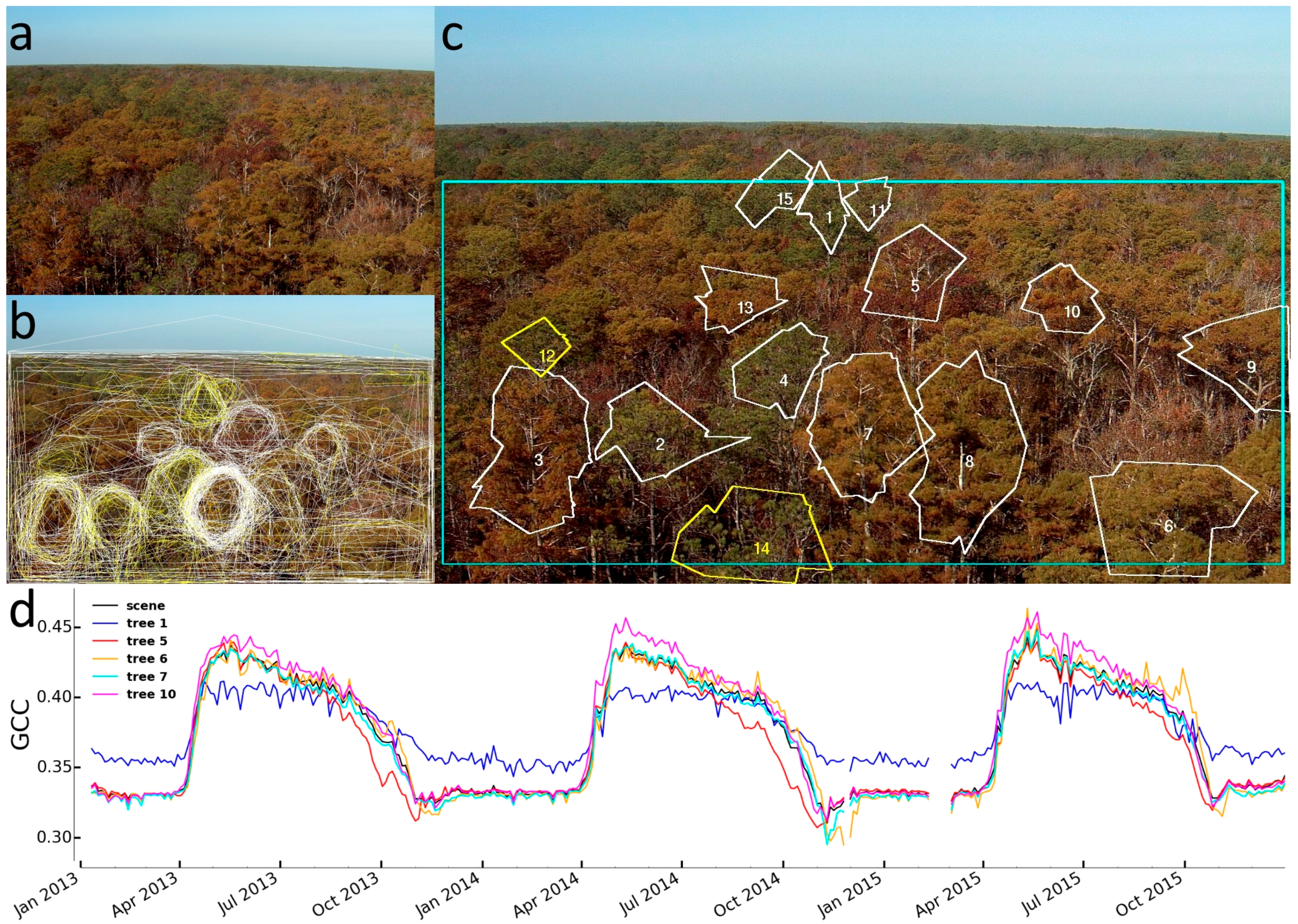
2.3.2. Identification of Individual Trees

For forest images in which we asked volunteers to outline individual trees (Group 2), we combined classifications across images for the same camera with a steady field of view. Each classification consisted of one or more polygons drawn on the image. We ignored “polygons” that consisted of fewer than three points and those whose lines crossed one another. We also ignored large polygons covering 30% or more of the image area.
We determined the locations of trees by clustering polygons across classifications, using the centroid of each polygon as its point location and the Density-Based Spatial Clustering of Applications with Noise (DBSCAN) algorithm from the python package sklearn cluster [25]. DBSCAN works by taking a distance metric and a minimum samples metric and forming a cluster if there are least minimum samples points within distance from one another. Additional points are added to this cluster if they are at most distance far away from any cluster point. Any points that are farther away from all cluster points than distance are considered outliers that do not belong to any cluster. For each of our sites, we set distance as proportional to the square root of the average area of all polygons being clustered. This ensured that bigger trees were properly grouped as single trees and that multiple smaller trees were not combined into a single cluster. For each site we set minimum samples as proportional to the square root of the number of total polygons being aggregated. This ensured that a reasonable fraction of volunteers had outlined a given tree, but that the threshold number of classifications for a particular tree was not too high for sites that had fewer overall classifications. See Supplementary Table S1 for a table of parameters used.
Once clusters were determined, we calculated the outline of the aggregated shape by taking the union of the n smallest polygons, where n is the maximum of 3% and 10% of comprising polygons. Our aggregated shapes are biased small purposely so that in using them to calculate GCC for a particular tree we do not include pixels from outside the target tree. Finally, we calculated the consensus label for each aggregated shape (broadleaf or needle leaf) by taking the majority vote of the labels for all polygons that had contributed to the aggregated shape. Each shape was then used as an image mask to calculate the GCC time series for individual trees. We used the standard formula, G C C = G R + G + B , where R, G, and B refer to red, green, and blue pixel values respectively, to calculate the greenness of each tree on each day; see [18] for implementation details.

2.3.3. Determination of Spring and Autumn Phenophase Transition Dates

For spring and autumn paired images (Group 3), we transformed the raw classifications by assigning a category to each classification. Classifications in which one or both of the images were described as poor were categorized as “bad image.” For spring images, classifications in which volunteers chose the image from a later date as the one having more or bigger green leaves, we categorized as “change detectable.” And classifications in which volunteers described the images as being the same or chose the image from a former date as the one having more or bigger green leaves, we categorized as “no change detectable.” For autumn images, we considered two types of phenophase transitions separately. Classifications in which volunteers chose images from an earlier date as having more leaves were categorized as “change detectable” for leaf fall, and those in which the earlier date was classified as having a greater proportion of green leaves were categorized as “change detectable” for color change. In both cases, when volunteers described image pairs as being the same or indicated the later date as having more leaves or a greater proportion of green leaves, the classifications were categorized as “no change detectable.” We then performed the following analyses separately for spring, autumn leaf fall, autumn color change, and for each set of images in which image pairs were one, three, or seven days apart.
For each date, we tallied up the number of classifications in each category across all image pairs that contained that date. For image sets that consisted of image pairs one day apart, each date consisted of classifications from exactly one image pair. But for image sets that consisted of image pairs three or seven days apart, most dates consisted of classifications across multiple image pairs. This “smoothing” of the classification data helped compensate for dates that had poor visibility (leading to “bad image” classifications), those that had unusual classifications compared to surrounding dates, and those that had missing images.
We then fit two step functions through each spring at each site, separately for image pairs one, three, and seven days apart. We first discarded all classifications from dates in which a majority of classifications resulted in “bad image”. We then assigned the value zero to each classification in the “no change detectable” category and the value one to each classification in the “change detectable” category. Our first step function began with the zero value, indicating that phenological change is not perceivable (e.g., when leaves are not on trees), and moved to one at the date of phenophase transition (e.g., leaf-out). The second step function began at one and then reverted to zero at the next phenophase transition (e.g., when leaves are at their fullest and change is no longer perceivable). The transition date of the second step function was required to be on or after that of the first step function. The linked step functions were fit with ordinary least squares to achieve a maximal fit. The result of the step functions was a pair of dates: the first day the step function has the value one (start of spring, start of leaf fall, start of leaf color change) and the last day the step function has the value one (end of spring, end of leaf fall, end of leaf color change).
We then evaluated the goodness of fit (GF) of the linked step functions using a determination coefficient calculated in a similar way to the R2 of linear regression. Specifically, we used the horizontal line x = 0 as our baseline and calculated the total sum of squares as the sum of the square of the distance of each y value (0 or 1) from this horizontal line. GF was then simply 1 − (residual sum of squares/total sum of squares). GF ranges from 0 to 1, with 0 indicating that the step function fits no better than the horizontal line at 0 and 1 indicating a perfect fit to data.
To estimate model uncertainty, we performed a bootstrap analysis with 100 replicates. For every image pair, we re-drew classifications from the pool of all classifications for that image pair, with replacement. We then performed the transformations, smoothing, and linked-step function fitting as described above for each replicate. We report the 95% confidence interval for all phenology transition dates from these replicates.

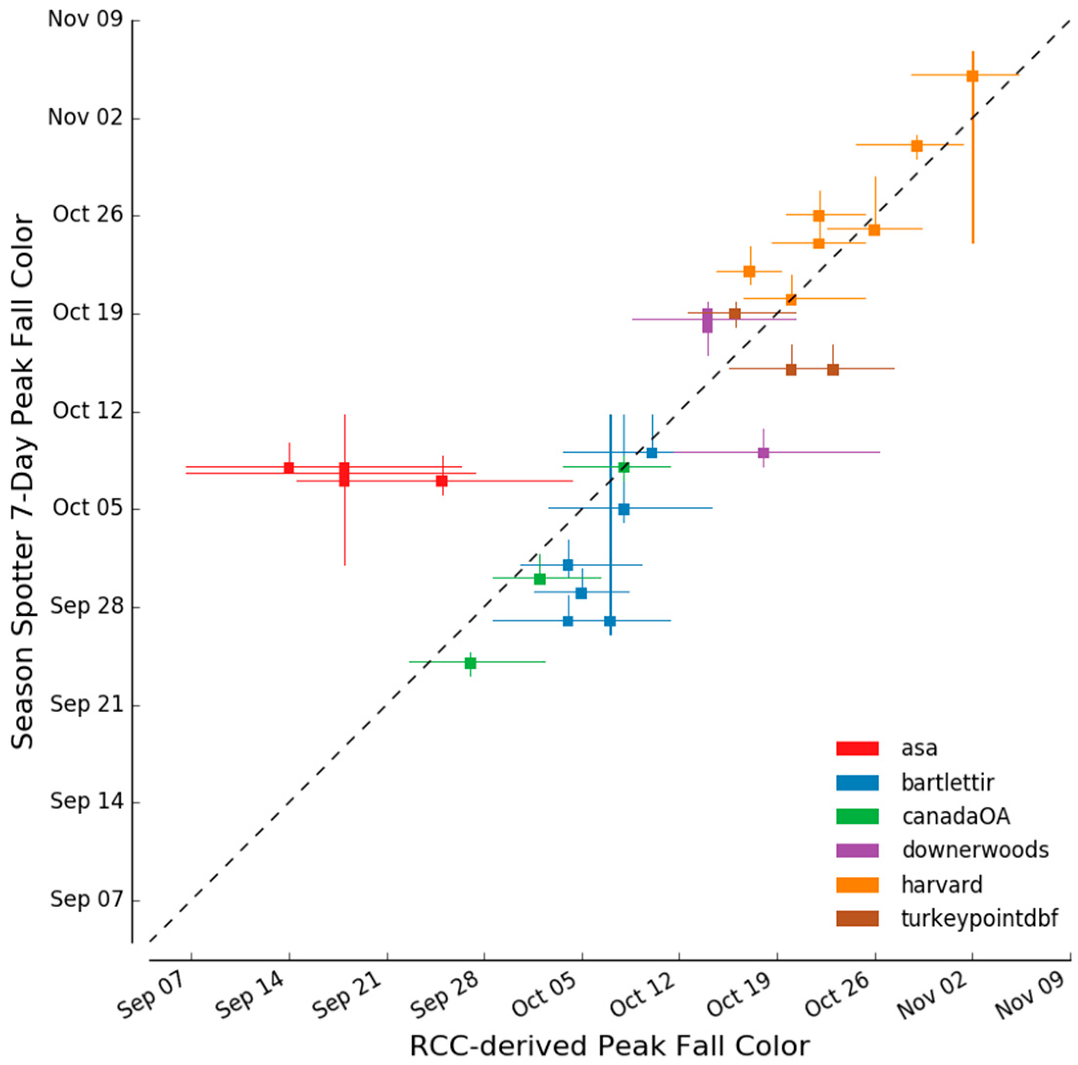
2.3.4. Determination of Autumn Peak Color

The autumn “peak color” date was calculated in a similar manner as autumn and spring transition dates. Image pairs in which the later image was considered to have better autumn colors were assigned the value 1, and image pairs in which the earlier image was considered to have better autumn colors were assigned the value 0. Image pairs in which the images were considered the same were ignored. We smoothed the classifications as described above and then fit a single step function by minimizing least squares, as above. We calculated the GF measure and ran a bootstrap analysis to assess uncertainty.

2.3.5. Comparison of Season Spotter Spring and Autumn Transition Dates with Those Derived from Automated GCC Measures

We compared “start of spring” and “end of spring” dates with those derived directly from GCC measures. First, we fit a spline to the GCC values at a given site in a given year using local regression (R function loess; [26]). The degree of smoothing was chosen based on the Bayesian Information Criterion (BIC) to create the best fit to the GCC data without overfitting. We then took the date where the spline reaches the 10% and 90% of total spline amplitude as the “start of spring” and “end of spring” dates. These percentages worked consistently well across all PhenoCam sites by avoiding noise at the start- and end-of-spring dates that led to large uncertainties [19]. We calculated the average difference between the dates derived from Season Spotter and those derived from GCC for each site-year.
To better estimate start-of-spring from GCC data, we then compared the Season Spotter start-of-spring dates to estimates that use from 5% to 25% of GCC amplitude to see if a different percentage would yield better agreement.
We compared start-of-color-change and end-of-color-change dates with those derived from GCC measures. We used the same spline function and 10% and 90% amplitudes for autumn. We calculated the average difference between Season Spotter date estimates and those derived from GCC values, as with spring.

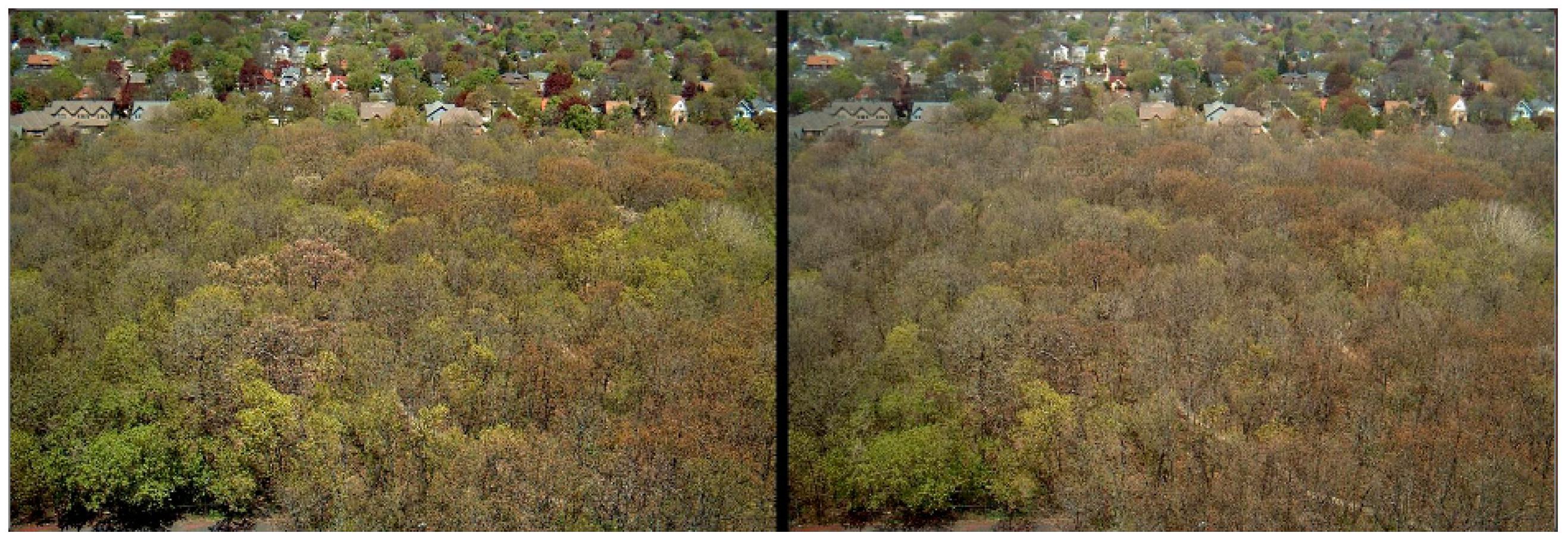
2.3.6. Analysis of Left-Right Bias in Classification of Image Pairs

Because the order in which paired images are shown to volunteers might affect their classifications, we showed each pair of spring and autumn images in both orientations (i.e. earlier day first and earlier day second). To detect any existing left–right bias, we removed all date pairs that were classified as “bad image” or “images are the same” by all volunteers. We then conducted a paired t-test on the number of classifications received for the earlier date of the pair depending on whether that image was on the left or the right. We also conducted a paired t-test on the number of classifications received for the later date of the pair. (Because “the images are the same” was an option, these two t-tests are independent.) We conducted these paired t-tests separately for spring, autumn color change, autumn leaf fall, and autumn peak color.

3. Results

By 12 May 2016, ~6000 registered volunteers and an additional ~12,000 unregistered volunteers contributed ~150,000 classifications to Season Spotter across all workflows. We use classifications up through this date in our analyses, though volunteers continued to classify images on Season Spotter. On average, Season Spotter received 833 ± 2381 (mean ± 1 SD) classifications per day, with a peak of 32,059 classifications in a single day during a volunteer recruitment campaign [22].

3.1. Reproductive and Vegetative Phenophases, Snow, and Image Quality

Season Spotter volunteers were able to identify peak flowering times (95% accuracy when compared with the gold standard validation dataset) and cone production (92% accuracy) across sites as well as crop states for corn and soybean (98% accuracy) (Figure 6, Figure 7 and Figure 8; Supplementary Figure S2). Our detailed inspection of individual images at a higher resolution than that presented to volunteers indicated that Season Spotter estimates of initial vegetative growth, flowering, and cone production often trailed actual dates by up to several days. Reliable identification of the presence of grass seedheads was not generally successful; consensus classifications of grass seedheads were often scattered throughout the year in sites known to have seasonal seeding such that inference of actual seeding events was not possible. Combined volunteer classifications accurately indicated whether snow was present and whether an image was of too poor quality to be used for further classification (98% accuracy) (Supplementary Figures S3 and S4).

3.2. Identification of Individual Trees

Volunteers were able to consistently draw outlines around individual trees of different sizes and shapes. Although we did not specify which trees to outline and we told volunteers that they need not outline more than three trees per image, we found that volunteers outlined a range of different types of trees at different distances from the camera. The result of combining volunteer classifications was multiple outlines per camera view, capturing a diversity of tree types in each view. Clustering of tree outlines resulted in combined shapes that visually reflect individual trees, while ignoring spurious shapes drawn by a few volunteers (Figure 9a–c). These shapes usually have the correct tree type identification (broadleaf or needle-leaf). Calculating GCC curves for these individual trees results in curves typical for broadleaf and needle-leaf trees [17] with variation seen among trees of the same type, as well as within species (Figure 9d).

3.3. Spring and Autumn Phenophase Transitions

When shown side-by-side images, volunteers were significantly more likely to choose the right image in a spring pair as having “more green leaves” whether that image was the chronologically earlier of the pair (p < 0.0001) or chronologically later (p < 0.0001). However, there was no detectable bias for left or right images for the autumn questions of leaf color change, leaf drop, and peak autumn color.
Volunteer classifications from image pairs seven and three days apart resulted in reasonable estimates of start of spring and end of spring (Figure 10 and Figure S5). Image pairs seven days apart provided estimates with lower uncertainty than those three days apart, because of higher agreement among volunteers. Image pairs one day apart resulted in poor estimates, with estimates near the middle of spring (when day-to-day phenology progression is most apparent) and large uncertainties. We were unable to calculate reliable transition dates from GCC time series for the underhill site, because this site does not use standard PhenoCam protocols to set a fixed white balance for all images; as a result, underhill GCC time series are very noisy. While Season Spotter estimates appear visually reasonable for the underhill site (Supplementary Figure S5), we had to omit from analysis comparisons between dates derived from Season Spotter and GCC time series.
Start-of-spring estimates using image pairs seven days apart tended to indicate an earlier date than the GCC-derived measures at 10% amplitude (bias: 0.69 days) with a mean absolute error of 4.77 days and an RMSD: 7.62 (Figure 11a). End-of-spring estimates tended to indicate a later date than GCC-derived measures at 90% amplitude (bias: 0.58 days) with a mean absolute error of 3.04 days and an RMSD of 3.85 (Figure 11b).
When we recalculated start-of-spring dates for GCC using different amplitude thresholds, we found that the best match to the Season Spotter estimate was at 15% amplitude (mean absolute difference 4.31 days). Amplitudes between 10% and 20% provided reasonable estimates (Supplementary Figure S7), while amplitudes below 10% greatly increased the estimated uncertainty.
As with spring, using image pairs seven days apart resulted in better estimates of autumn color change, leaf drop, and peak autumn color with smaller uncertainties than image pairs three days apart. Likewise, image pairs one day apart resulted in poor estimates. Start-of-color-change estimates using image pairs seven days apart indicated much later start-of-autumn dates, a narrower range and narrower uncertainties than the GCC-derived measures at 90% amplitude (mean absolute error: 52.1 days; RMSD: 60.4; bias 51.7 days; Figure 11c). End-of-color-change estimates tended to be later than GCC-derived measures at 10% amplitude (bias: 1.35 days) by a mean absolute difference of 9.50 days (RMSD: 14.1). Season Spotter estimates for one site, asa, were substantially earlier than GCC-derived estimates (Figure 11d).
Peak leaf color estimates using image pairs seven days apart corresponded closely to the maximum value of a redness vegetation index (“red chromatic coordinate”; R C C = R R + G + B , where R, G, and B refer to red, green, and blue pixel values respectively; [18]) across sites (mean absolute difference: 5.60 days, RMSD: 7.96, bias: 0.72 days) (Figure 12). Sites dominated by red-leaved species, such as red maples at the harvard site, matched particularly well, whereas sites dominated by yellow-leaved species, such as silver birch at the asa site, showed less agreement.

4. Discussion

We engaged citizen science volunteers to successfully extract information from phenology camera imagery that cannot presently be extracted automatically. This information included vegetative and reproductive states of landscape vegetation, occurrence of snow, and the locations of individual trees. Additionally, we used citizen science to ground-truth automated algorithms that determine the start and end of spring and autumn dates directly from phenology camera imagery. Here we discuss possible applications for phenology data produced by citizen science data-processing projects like Season Spotter and provide guidance for the design and implementation of future image-based online citizen science projects.

4.1. Applications for Season Spotter Data

4.1.1. Direct Use for Biological Research

Data on plant phenology from Season Spotter and other future similar citizen science projects complement that of remote sensing vegetation indices and ground phenology observation efforts like those of the USA National Phenology Network [27] and Project Budburst [28]. They can be used directly to research the effects and drivers of climate change on plant vegetation and reproductive state. It is clear, for example, that a warming climate is affecting the leaf-out and leaf senescence of species at different rates [2,3]. The granularity of Season Spotter data allows for tracking individual species at high temporal resolution. In combination with other phenology data, Season Spotter data can also be used to examine potential phenology mismatch between plants and animals as a result of environmental change at high temporal resolution. And they can be used by land managers for monitoring and management purposes.

4.1.2. Connecting Between Ground Phenology Data and Satellite Sensed Phenology Data

PhenoCam imagery offers the potential to conduct analyses across a range of spatial scales. It is possible to calculate vegetation indices as well as track the phenology of individual trees and the canopy as a whole. This provides a unique opportunity to connect the biology of individuals to landscape-level measures of phenology. Using outlines drawn by volunteers in Season Spotter, we were able to produce phenology time series for individual trees (Figure 9). These seasonal trajectories show the expected general shape for broadleaf trees (sharp increase in spring, followed by gradual summer decline, and ending in sharp decrease in autumn) and needle-leaf trees (gradual increase at the beginning of the growing season and gradual decrease at the end of it). However, individual trajectories vary in their exact shape and peak amplitude (Figure 9d). This suggests that decomposing landscapes into individual trees can help bridge scales of observation from the individual to the landscape, providing insight into sub-pixel heterogeneity that is an inevitable consequence of coarse-resolution satellite remote sensing. For example, we can discern to what extent the start of spring, as derived from vegetation indices, is driven by early leafing species. We can better understand how two distinctly different processes of senescence—leaf color change and leaf fall—combine to produce remotely sensed vegetation indices in autumn [29]. And we can quantify how the phenological variation among individuals is perceived by satellite sensors that combine the phenology of hundreds or thousands of individuals into a single multi-meter pixel [30].

4.1.3. Validating Vegetation Indices

Data from Season Spotter and similar projects can also be used to validate satellite remote sensing data. While ground-based measures of phenology can provide a spatially extensive sampling of species for comparison with satellite sensor data (e.g., [31]), PhenoCam images and Season Spotter data provide high temporal resolution for such comparisons. Our analyses of spring and autumn phenological transition dates of deciduous forests shows that citizen science in combination with phenology cameras can help connect biological-based observations with inferences made about phenology from vegetation indices.
In Season Spotter, volunteers could tell when leaves appear on the trees, when tree canopies are fully developed, when leaves begin to change color, when they begin to fall, and when leaf fall was complete. The transition date showing the most variation between Season Spotter estimates and GCC-derived estimates was the beginning of autumn color change. The Season Spotter estimates were more biologically reasonable, given their tighter range (mid-August to end of September vs. mid-June to early September) and the large uncertainties in the GCC-derived estimates. Visual inspection of GCC curves indicated that Season Spotter estimates occur near inflection points where GCC values start decreasing rapidly (Supplementary Figure S6). Additionally, Season Spotter estimates for the harvard site were within a few days of the long-term mean date of autumn color change based on ground-based measures [32]. One challenge in using the 90% amplitude of GCC is that summertime GCC values slowly decrease, before decreasing more rapidly in autumn. Depending on the amplitude of the summer decrease, the 90% amplitude metric may occur during mid-summer instead of at the end of it. A more sophisticated GCC algorithm that takes into account the curvature and/or slope of the GCC curve may be better at estimating the actual start-of-color-change. Thus, data from Season Spotter can provide important biological insight that will help to improve phenophase detection algorithms currently being used and ensure that the derived transition dates correspond directly to biologically relevant changes occurring on the ground.
Season Spotter data may be particularly helpful in validating the biological interpretation of autumn from remote sensing. The calculated end-of-leaf-color-change date was typically associated with the autumn nadir of the GCC time series for each site-year. At some sites, such as harvard, this GCC minimum is followed by a slight rise to a winter baseline. Biologically, the GCC minimum corresponds with peak red leaf color, and then GCC rises as leaves are shed and the scene becomes less red (Supplementary Figure S6). The calculated end-of-leaf-fall dates for these sites typically coincide with the return to the winter baseline. For sites dominated by trees that turn red in the autumn, the date of peak autumn color corresponded well with the maximum value of RCC, the red analogy to GCC [18]. These correlations suggest that vegetation indices can be used to infer specific biological events such as end of leaf color change, end of leaf fall, and peak autumn color rather than simple start-, mid-, and end-of-autumn transition dates. However, the exact interpretation will depend on the dominant species at each site and the color of those species’ leaves in autumn. For example, an index based on “yellowness” would work better than RCC at sites like asa.
The agreement between Season Spotter estimates and those derived from GCC for most, but not all, transition dates indicates that estimates derived from phenology camera imagery and citizen science can play an important role in evaluating remote sensing algorithms and suggesting refinements. Using Season Spotter estimates as ground-truthing values for GCC estimates suggests that transition dates derived from spline-fitting of vegetation indices can be reasonably interpreted to indicate the start and end of spring green-up and end of leaf color change in autumn for temperate deciduous forests. Because transition dates from GCC also correlate with NDVI and EVI derived from MODIS and Landsat imagery [19,33,34], citizen science data based on phenology camera imagery may be used to provide a biological basis for interpretation of satellite vegetation indices, too.

4.1.4. Improving Automated Processing of Remote Sensing Data

In addition to validating existing vegetation index algorithms, data from Season Spotter and similar projects can be used to refine automated data-management pipelines. For example, removal of images judged by volunteers as poor quality or snowy removes noise and bias from GCC time series. Similarly, sites that have extensive flowering events sometimes show abnormal deviations in their GCC time series; these events can be noted by citizen scientists to allow for investigation and correction.
Volunteer classifications for data-processing citizen science projects like Season Spotter can also be used for the construction of automated data flows to allow for scaling to large networks of remote sensors. While it is currently necessary to involve human volunteers in the detection of flowers in PhenoCam images, for example, computers can be trained to do the same task. Machine-learning algorithms provide a means for automating processing of complex images, but they typically depend on large annotated datasets to learn automated classification tasks [35]. The datasets that volunteers create in such projects as Season Spotter can then be used to train such algorithms to enable automated classification.
These large annotated image sets might also be used in computer vision research to better enable computers to recognize environmental landscapes and features. Current research on outdoor computer vision relies on large compendiums of crowdsourced images. However state-of-the-art deep-learning algorithms fail to properly classify landscape types and features that are poorly represented in those images (e.g., tundra). Phenology cameras can provide large quantities of images of diverse and heterogeneous environments, while citizen scientists can provide the labels needed to train computers to recognize the Earth environment.

4.2. Recommendations for Citizen Science Data Processing of Remote Sensing Imagery

Building an online citizen science project for data processing of images has never been easier. Using the Zooniverse Project Builder (www.zooniverse.org/lab), it is possible to prototype a new project in under an hour [21]. Currently, the Project Builder supports single-answer and multiple-answer questions and drawing tasks. The next step is creating project content: the full text and many images necessary for task completion as well as help, tutorial, and educational materials. Beta testing the project, potentially multiple times, is vital to ensure high quality and usability of the resulting classifications [36,37]. For example, Mountain Watch, a ground-based phenology citizen science project, found that initial identifications by volunteers were inconsistent, due to misidentification of species or inaccurate location descriptions. Consequently, the project altered its methods to use permanent plots and better-trained personnel [38]. As it is for any citizen science project, the main ongoing investment is recruiting, retaining, and communicating with volunteers as well as in good data-management practices [39,40].
Season Spotter was successful in engaging volunteers and producing valuable data by following some straightforward guidelines [22,41]. We ensured that our questions were short, simply worded, and lacked jargon. We provided comprehensive supplementary material behind “help” buttons. This material included example images, additional instructional text, and directions on what to do if an unusual image was presented. We also provided background and reference materials so that volunteers understood how they were contributing to science and could explore plant phenology in more depth. Importantly, we maintained communication with volunteers throughout, from initial testing of the project throughout its running. This allowed us to incorporate feedback into the project design initially and alerted us when volunteers were having difficulty with particular question types. Crall et al. found partnering with organizations that share common goals to reach a broad audience was key for recruiting volunteers and that ongoing engagement of existing volunteers was important for volunteer retention [22].
We learned that Season Spotter was not as efficient as it might have been, though. Ideally, citizen science projects should be set up to maximize volunteer effort and speed data-classification time. Having multiple volunteers classify every available image decreases random error, but increases the amount of overall volunteer effort required. For data that are temporally correlated, it may be possible to exclude sets of images and subsample from the rest. For example, if one were only interested in extracting reproductive states from vegetation at a site where plants flower only in summer, weeks that have daily temperatures always below freezing can be excluded before sending images to volunteers. Another strategy might be to initially present only every fifth image to volunteers when a phenological state such as flowering typically happens over several days or weeks. Then a second round of classification could be conducted consisting of only the unused images immediately before and after those that were positively classified as flowering. For a site in which flowering lasts two weeks out of the year, this method would require just 25% of the effort needed to inspect every image over the year. A more advanced approach might use machine-learning algorithms to provide initial classifications and then ask volunteers to weigh in on images for which the algorithm has low certainty.
Another area for ongoing online citizen science research is in design techniques for sustaining volunteer interest and engagement [42]. While we actively engaged with volunteers on social media and in a dedicated chat forum, we found that Season Spotter’s volunteer retention rate was somewhat lower than those of other Zooniverse projects. We believe that this may have been due to a lack of variety in images seen by volunteers. In order to develop full datasets per site, we selected a subset of PhenoCam sites to use in Season Spotter. This meant that our volunteers saw images from the same sites repeatedly, potentially leading to boredom, as was suggested by some volunteer comments in the chat forum. Future projects may want to assess volunteer response to image variety during beta testing. Exactly how to balance volunteer interest with researcher data needs is a topic in need of more research.
Citizen science projects analyzing remote sensing imagery will need to take into account the size of the features to be classified relative to the full image and the viewing device used by volunteers. In Season Spotter, volunteers were often able to accurately classify flowers and cones in images (Figure 6, Figure 7, Figure 8 and Figure S2), but they were unable to correctly identify images containing small grass seedheads. Additionally, images containing very few flowers were sometimes misclassified as not having any flowers. Because PhenoCam images comprise entire landscapes, extraction of information about small features such as flowers and seeds is likely going to succeed or fail based on the size of the individual features relative to the size of the whole image and the pixel resolution of the image (as is the case for all fine-scale remote sensing [43]). For example, volunteers were able to identify cones in a hemlock forest. However, the most easily seen cones were quite close to the camera and therefore reasonably large relative to image size (Supplementary Figure S2). A similar view that contained only trees farther away would have been more difficult for volunteers, and it is likely that the rate of cone detection would have dropped. By contrast, the reproductive phenology of monocultures like crops may be obvious to volunteers, even if individual flowers or seeds are relatively small; volunteers were readily able to differentiate vegetative and reproductive stages of corn and soybean (Figure 8).
On average, volunteers viewed images at 40% their original resolution, due to device and browser limitations. Several volunteers noted in the Season Spotter discussion forum that the size of the images made it difficult to see small features like flowers and cones, and they requested a zoom tool that would magnify images on-screen so that they could more carefully inspect images. Such a tool must be considered carefully, because it presents the dilemma that all volunteers may not see the same things when viewing the same image, potentially biasing the resulting data. Recording whether or not each volunteer uses such a zoom tool may help to properly combine classifications. Another method for increasing the ability for volunteers to correctly identify small features is to pre-select a region of the full landscape image that is likely to contain those features and then crop images to just this region, in effect automatically zooming in for all volunteers. The amount of zoom that can be achieved will ultimately be limited by the resolution of the initial image; higher-resolution images are more likely to elicit good citizen science classifications for small things like flowers and cones than lower-resolution ones.
As with all scientific endeavors, it is important for citizen science projects to assess the quality of collected data and account for bias [36]. In Season Spotter, we found a tendency for volunteers to select the right-hand image when presented paired images for one spring question, but not three autumn questions. We were able to avoid bias in the resulting spring data by showing every set of paired images in both orientations, and we suggest all projects showing images side by side do likewise. Further research into the causes of perception bias in online citizen science projects would be valuable to help guide project design to ensure high data quality [44].
Citizen science for Earth observation at large spatial scales holds promise for increasing basic understanding of Earth’s biological and physical systems as well as advising management and policy objectives. Season Spotter and similar online data-processing citizen science projects make it feasible to analyze large image sets, whether they are from near-Earth sensors like phenology cameras, traditional satellite sensors like Landsat (e.g., [45]), or specialized picosatellite sensors. The resulting data can be used to support Earth observation for climate change research and land management both alone and in combination with satellite remote sensing.

5. Conclusions

Understanding the impacts of climate change on the phenology of Earth’s vegetation requires integrating complementary methods across scales ranging from local to regional. Near-surface phenology cameras collect data at an intermediate scale between those of field-based ground observations and satellite imagery, and networks of such cameras established across North America, Europe, Australia, and Japan are expanding [8]. Typically, vegetation indices are calculated from phenology camera imagery to infer changes in leaf area and photosynthesis over the seasons. Additional data exists in these images, but automated methods to extract them have not been developed, and the large volume of imagery makes it prohibitive for a single team of researchers to annotate them all by hand.
We found that citizen science was a practical solution for extracting this additional information from phenology camera imagery. In particular, volunteers could identify showy flowers, tree cones at a relatively close distance, and crop reproductive stages (but not grass seedheads) in landscape images. This reproductive information is a new data source that holds potential for understanding the impacts of climate change at broad spatial scales. Citizen scientists were also reliably able to outline individual trees, providing data for understanding how the vegetative phenology of individuals connects to the phenology of landscapes. And they provided information on the spring and autumn vegetation changes in deciduous forests that we used to calculate start and end of spring and autumn transition dates. These dates provide a biological basis for validating specific transition dates derived from continuous vegetation indices obtained from either near-surface phenological cameras or satellite remote sensing. Engaging citizen scientists to extract information from landscape phenology imagery is a promising approach to develop complementary phenology data, bridge scales, and validate vegetation indices.

Supplementary Materials

The following are available online at www.mdpi.com/2072-4292/8/9/726/s1, Table S1. Parameters used in the DBSCAN clustering algorithm; Figure S1. Season Spotter Workflows; Figure S2. Midday image from the harvardhemlock site showing cones visible; Figure S3. Examples of images classified as having snow; Figure S4. Examples of images classified as “bad image”; Figure S5. Estimates of start and end of spring from Season Spotter based on image pairs one, three, and seven days apart, as well as estimates derived from GCC values; Figure S6. Estimates of start and end of autumn color change, start and end of autumn leaf fall and peak color from Season Spotter based on image pairs seven days apart, as well as estimates of the start and end of autumn derived from GCC values; Figure S7. Mean days difference between estimates of start of spring derived from GCC values and calculated from Season Spotter data as a function of the amplitude used in the GCC-derived estimate.

Acknowledgments

This research would not have been possible without the more than 18,000 citizen science volunteers who provided classifications to Season Spotter (a full list of volunteer names is available online at http://seasonspotter.org/contributors.html); we are grateful for their time and enthusiasm. We also thank Steve Klosterman, Carolyn Gigot, Sarah Newman, and Kat Bevington for engaging with and encouraging volunteers through blog posts, forum conversations, and educational materials. Tom Milliman and Dennis Ward provided invaluable data management and web development support respectively. We thank Jonathan Furst and Jim Williamson for identifying tree species at alligatorriver and PhenoClub members for ongoing constructive feedback. Season Spotter was developed through grant EF-1065029 from the National Science Foundation through the Macrosystems Biology Program. Imagery and data from the PhenoCam project are publicly available online at phenocam.sr.unh.edu. We thank the PhenoCam site collaborators for their support of the PhenoCam network. This publication uses data generated via the Zooniverse.org platform, development of which was supported by a Global Impact Award from Google and by the Alfred P. Sloan Foundation.

Author Contributions

We use the CRediT taxonomy of contribution types. Conceptualization: Margaret Kosmala, Rebecca Cheng, Sandra Henderson, Andrew D. Richardson; Methodology, Investigation: Margaret Kosmala, Rebecca Cheng, Alycia Crall, Koen Hufkens; Software: Margaret Kosmala, Koen Hufkens; Formal Analysis, Data Curation, Writing—Original Draft Preparation: Margaret Kosmala; Writing—Review and Editing: Margaret Kosmala, Alycia Crall, Rebecca Cheng, Koen Hufkens, Sandra Henderson, Andrew D. Richardson; Visualization: Margaret Kosmala, Alycia Crall; Supervision, Funding Acquisition: Andrew D. Richardson, Sandra Henderson.

Conflicts of Interest

The authors declare no conflict of interest.

Abbreviations

The following abbreviations are used in this manuscript:
NDVInormalized difference vegetation index
EVIenhanced vegetation index
MODISmoderate-resolution imaging spectroradiometer
GCCgreen chromatic coordinate
RCCred chromatic coordinate
DBSCANdensity-based spatial clustering of applications with noise
GFgoodness of fit
RMSDroot-mean-square deviation

References

  1. Richardson, A.D.; Keenan, T.F.; Migliavacca, M.; Ryu, Y.; Sonnentag, O.; Toomey, M. Climate change, phenology, and phenological control of vegetation feedbacks to the climate system. Agric. For. Meteorol. 2013, 169, 156–173. [Google Scholar] [CrossRef]
  2. Ibáñez, I.; Primack, R.B.; Miller-Rushing, A.J.; Ellwood, E.; Higuchi, H.; Lee, S.D.; Kobori, H.; Silander, J.A. Forecasting phenology under global warming. Philos. Trans. R. Soc. B Biol. Sci. 2010, 365, 3247–3260. [Google Scholar] [CrossRef] [PubMed]
  3. Menzel, A.; Sparks, T.H.; Estrella, N.; Koch, E.; Aasa, A.; Ahas, R.; Alm-Kübler, K.; Bissolli, P.; Braslavská, O.; Briede, A.; et al. European phenological response to climate change matches the warming pattern. Glob. Chang. Biol. 2006, 12, 1969–1976. [Google Scholar] [CrossRef]
  4. Garonna, I.; de Jong, R.; de Wit, A.J.W.; Mücher, C.A.; Schmid, B.; Schaepman, M.E. Strong contribution of autumn phenology to changes in satellite-derived growing season length estimates across Europe (1982–2011). Glob. Chang. Biol. 2014, 20, 3457–3470. [Google Scholar] [CrossRef] [PubMed]
  5. Keenan, T.F.; Richardson, A.D. The timing of autumn senescence is affected by the timing of spring phenology: implications for predictive models. Glob. Chang. Biol. 2015, 21, 2634–2641. [Google Scholar] [CrossRef] [PubMed]
  6. Cleland, E.E.; Chuine, I.; Menzel, A.; Mooney, H.A.; Schwartz, M.D. Shifting plant phenology in response to global change. Trends Ecol. Evol. 2007, 22, 357–365. [Google Scholar] [CrossRef] [PubMed]
  7. Pettorelli, N.; Vik, J.O.; Mysterud, A.; Gaillard, J.-M.; Tucker, C.J.; Stenseth, N.C. Using the satellite-derived NDVI to assess ecological responses to environmental change. Trends Ecol. Evol. 2005, 20, 503–510. [Google Scholar] [CrossRef] [PubMed]
  8. Brown, T.B.; Hultine, K.R.; Steltzer, H.; Denny, E.G.; Denslow, M.W.; Granados, J.; Henderson, S.; Moore, D.; Nagai, S.; SanClements, M.; et al. Using phenocams to monitor our changing Earth: Toward a global phenocam network. Front. Ecol. Environ. 2016, 14, 84–93. [Google Scholar] [CrossRef]
  9. Huete, A.; Didan, K.; Miura, T.; Rodriguez, E.P.; Gao, X.; Ferreira, L.G. Overview of the radiometric and biophysical performance of the MODIS vegetation indices. Remote Sens. Environ. 2002, 83, 195–213. [Google Scholar] [CrossRef]
  10. Morisette, J.T.; Richardson, A.D.; Knapp, A.K.; Fisher, J.I.; Graham, E.A.; Abatzoglou, J.; Wilson, B.E.; Breshears, D.D.; Henebry, G.M.; Hanes, J.M.; et al. Tracking the rhythm of the seasons in the face of global change: Phenological research in the 21st century. Front. Ecol. Environ. 2009, 7, 253–260. [Google Scholar] [CrossRef]
  11. Badeck, F.-W.; Bondeau, A.; Bottcher, K.; Doktor, D.; Lucht, W.; Schaber, J.; Sitch, S. Responses of spring phenology to climate change. New Phytol. 2004, 162, 295–309. [Google Scholar] [CrossRef]
  12. Crimmins, M.A.; Crimmins, T.M. Monitoring plant phenology using digital repeat photography. Environ. Manag. 2008, 41, 949–958. [Google Scholar] [CrossRef] [PubMed]
  13. Wiggins, A.; Crowston, K. From conservation to crowdsourcing: A typology of citizen science. In Proceedings of 44th Hawaii International Conference on System Sciences (HICSS), Kauai, HI, USA, 4–7 January 2011; pp. 1–10.
  14. Lintott, C.J.; Schawinski, K.; Slosar, A.; Land, K.; Bamford, S.; Thomas, D.; Raddick, M.J.; Nichol, R.C.; Szalay, A.; Andreescu, D.; et al. Galaxy Zoo: Morphologies derived from visual inspection of galaxies from the Sloan Digital Sky Survey. Mon. Not. R. Astron. Soc. 2008, 389, 1179–1189. [Google Scholar] [CrossRef] [Green Version]
  15. Westphal, A.J.; Stroud, R.M.; Bechtel, H.A.; Brenker, F.E.; Butterworth, A.L.; Flynn, G.J.; Frank, D.R.; Gainsforth, Z.; Hillier, J.K.; Postberg, F.; et al. Evidence for interstellar origin of seven dust particles collected by the Stardust spacecraft. Science 2014, 345, 786–791. [Google Scholar] [CrossRef] [PubMed]
  16. Swanson, A.; Kosmala, M.; Lintott, C.; Packer, C. A generalized approach for producing, quantifying, and validating citizen science data from wildlife images. Conserv. Biol. 2016, 30, 520–531. [Google Scholar] [CrossRef] [PubMed]
  17. Richardson, A.D.; Braswell, B.H.; Hollinger, D.Y.; Jenkins, J.P.; Ollinger, S.V. Near-surface remote sensing of spatial and temporal variation in canopy phenology. Ecol. Appl. 2009, 19, 1417–1428. [Google Scholar] [CrossRef] [PubMed]
  18. Sonnentag, O.; Hufkens, K.; Teshera-Sterne, C.; Young, A.M.; Friedl, M.; Braswell, B.H.; Milliman, T.; O’Keefe, J.; Richardson, A.D. Digital repeat photography for phenological research in forest ecosystems. Agric. For. Meteorol. 2012, 152, 159–177. [Google Scholar] [CrossRef]
  19. Klosterman, S.T.; Hufkens, K.; Gray, J.M.; Melaas, E.; Sonnentag, O.; Lavine, I.; Mitchell, L.; Norman, R.; Friedl, M.A.; Richardson, A.D. Evaluating remote sensing of deciduous forest phenology at multiple spatial scales using PhenoCam imagery. Biogeosciences 2014, 11, 4305–4320. [Google Scholar] [CrossRef]
  20. Toomey, M.; Friedl, M.A.; Frolking, S.; Hufkens, K.; Klosterman, S.; Sonnentag, O.; Baldocchi, D.D.; Bernacchi, C.J.; Biraud, S.C.; Bohrer, G.; et al. Greenness indices from digital cameras predict the timing and seasonal dynamics of canopy-scale photosynthesis. Ecol. Appl. 2015, 25, 99–115. [Google Scholar] [CrossRef] [PubMed]
  21. Bowyer, A.; Lintott, C.; Hines, G.; Allen, C.; Paget, E. Panoptes, a project building tool for citizen science. 2015; in press. [Google Scholar]
  22. Crall, A.W.; Kosmala, M.; Cheng, R.; Brier, J.; Cavalier, D.; Henderson, S.; Richardson, A.D. Marketing online citizen science projects to support volunteer recruitment and retention: Lessons from season spotter. PLOS ONE 2016. under review. [Google Scholar]
  23. Keenan, T.F.; Darby, B.; Felts, E.; Sonnentag, O.; Friedl, M.A.; Hufkens, K.; O’Keefe, J.; Klosterman, S.; Munger, J.W.; Toomey, M.; et al. Tracking forest phenology and seasonal physiology using digital repeat photography: A critical assessment. Ecol. Appl. 2014, 24, 1478–1489. [Google Scholar] [CrossRef]
  24. Richardson, A.D.; Jenkins, J.P.; Braswell, B.H.; Hollinger, D.Y.; Ollinger, S.V.; Smith, M.-L. Use of digital webcam images to track spring green-up in a deciduous broadleaf forest. Oecologia 2007, 152, 323–334. [Google Scholar] [CrossRef] [PubMed]
  25. Pedregosa, F.; Varoquaux, G.; Gramfort, A.; Michel, V.; Thirion, B.; Grisel, O.; Blondel, M.; Prettenhofer, P.; Weiss, R.; Dubourg, V.; et al. Scikit-learn: Machine learning in Python. J. Mach. Learn. Res. 2011, 12, 2825–2830. [Google Scholar]
  26. Cleveland, W.S.; Grosse, E.; Shyu, W.M. Local regression models. In Statistical Models in S; Chambers, J.M., Hastie, T.J., Eds.; CRC Press: Boca Raton, FL, USA, 1992; Volume 2, pp. 309–376. [Google Scholar]
  27. Schwartz, M.D.; Betancourt, J.L.; Weltzin, J.F. From Caprio’s lilacs to the USA National Phenology Network. Front. Ecol. Environ. 2012, 10, 324–327. [Google Scholar] [CrossRef]
  28. Henderson, S.; Ward, D.L.; Meymaris, K.K.; Alaback, P.; Havens, K. Project Budburst: Citizen science for all seasons. In Citizen Science: Public Participation in Environmental Research; Dickinson, J.L., Bonney, R., Eds.; Cornell University Press: Ithaca, NY, USA, 2012; pp. 50–57. [Google Scholar]
  29. Gallinat, A.S.; Primack, R.B.; Wagner, D.L. Autumn, the neglected season in climate change research. Trends Ecol. Evol. 2015, 30, 169–176. [Google Scholar] [CrossRef] [PubMed]
  30. Liang, L.; Schwartz, M.D.; Fei, S. Validating satellite phenology through intensive ground observation and landscape scaling in a mixed seasonal forest. Remote Sens. Environ. 2011, 115, 143–157. [Google Scholar] [CrossRef]
  31. Elmore, A.; Stylinski, C.; Pradhan, K. Synergistic use of citizen science and remote sensing for continental-scale measurements of forest tree phenology. Remote Sens. 2016, 8, 502. [Google Scholar] [CrossRef]
  32. Richardson, A.D.; O’Keefe, J. Phenological differences between understory and overstory. In Phenology of Ecosystem Processes; Noormets, A., Ed.; Springer New York: New York, NY, USA, 2009; pp. 87–117. [Google Scholar]
  33. Hufkens, K.; Friedl, M.; Sonnentag, O.; Braswell, B.H.; Milliman, T.; Richardson, A.D. Linking near-surface and satellite remote sensing measurements of deciduous broadleaf forest phenology. Remote Sens. Environ. 2012, 117, 307–321. [Google Scholar] [CrossRef]
  34. Melaas, E.K.; Sulla-Menashe, D.; Gray, J.M.; Black, T.A.; Morin, T.H.; Richardson, A.D.; Friedl, M.A. Multisite analysis of land surface phenology in North American temperate and boreal deciduous forests from Landsat. Remote Sens. Environ. 2016, in press. [Google Scholar]
  35. Alpaydin, E. Introduction to Machine Learning; MIT Press: Cambridge, MA, USA, 2014. [Google Scholar]
  36. Kosmala, M.; Wiggins, A.; Swanson, A.; Simmons, B. Assessing data quality in citizen science. Front. Ecol. Environ. 2016, in press. [Google Scholar]
  37. Crall, A.W.; Newman, G.J.; Jarnevich, C.S.; Stohlgren, T.J.; Waller, D.M.; Graham, J. Improving and integrating data on invasive species collected by citizen scientists. Biol. Invasions 2010, 12, 3419–3428. [Google Scholar] [CrossRef]
  38. McDonough MacKenzie, C.; Murray, G.; Primack, R.; Weihrauch, D. Lessons from citizen science: Assessing volunteer-collected plant phenology data with Mountain Watch. Biol. Conserv. 2016, in press. [Google Scholar] [CrossRef]
  39. Michener, W.K.; Jones, M.B. Ecoinformatics: supporting ecology as a data-intensive science. Trends Ecol. Evol. 2012, 27, 85–93. [Google Scholar] [CrossRef] [PubMed]
  40. Wiggins, A.; Bonney, R.; Graham, E.; Henderson, S.; Kelling, S.; LeBuhn, G.; Litauer, R.; Lotts, K.; Michener, W.; Newman, G.; et al. Data Management Guide for Public Participation in Scientific Research; DataOne Working Group: Albuquerque, NM, USA, 2013; pp. 1–41. [Google Scholar]
  41. Zooniverse Best Practices. Available online: https://www.zooniverse.org/lab-best-practices/great-project (accessed on 12 July 2016).
  42. Cox, J.; Oh, E.Y.; Simmons, B.; Lintott, C.; Masters, K.; Greenhill, A.; Graham, G.; Holmes, K. Defining and measuring success in online citizen science: A case study of Zooniverse projects. Comput. Sci. Eng. 2015, 17, 28–41. [Google Scholar] [CrossRef]
  43. Blaschke, T. Object based image analysis for remote sensing. ISPRS J. Photogramm. Remote Sens. 2010, 65, 2–16. [Google Scholar] [CrossRef]
  44. Jordan, R.C.; Ehrenfeld, J.G.; Gray, S.A.; Brooks, W.R.; Howe, D.V.; Hmelo-Silver, C.E. Cognitive considerations in the development of citizen science projects. In Citizen Science: Public Participation in Environmental Research; Dickinson, J.L., Bonney, R., Eds.; Cornell University Press: Ithaca, NY, USA, 2012; pp. 167–178. [Google Scholar]
  45. Floating Forests. Available online: https://www.floatingforests.org/#/classify (accessed on 12 July 2016).
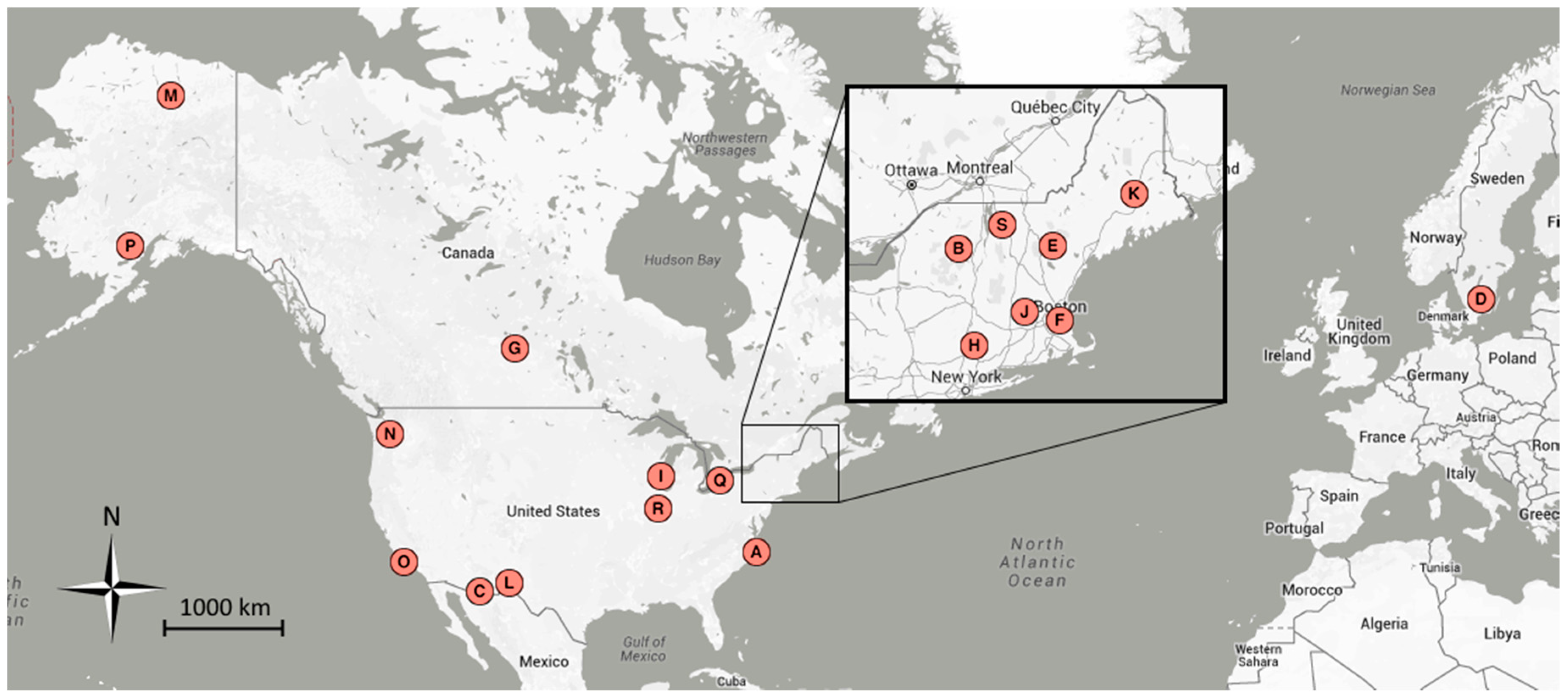
Figure 1. Examples of landscape images as seen by phenology cameras in the PhenoCam network. Shown are sites (a) jerbajada; (b) bartlettir; (c) snipelake; (d) arbutuslake; (e) downerwoods; (f) uiefmaize; (g) ibp; (h) mountranier; (i) bostoncommon. See Table 1 for site descriptions.
Remotesensing 08 00726 g001
Figure 2. The Season Spotter user interface.
Remotesensing 08 00726 g002
Figure 3. Workflow for PhenoCam images containing grass. See Supplementary Materials Figure S1 for all other workflows.
Remotesensing 08 00726 g003
Figure 4. Map of PhenoCam sites used in Season Spotter. See Table 1 for site descriptions.
Remotesensing 08 00726 g004
Figure 5. Example of paired images shown to volunteers in Season Spotter. These two images were taken in spring, seven days apart, at the downerwoods site. Green-up has progressed further in the left image.
Remotesensing 08 00726 g005
Figure 6. Midday images from the asa site in 2012; shown are (a) the full landscape view; and (bd) a sub-region enlarged to show shrub flowering detail; Season Spotter data indicated (a) mid-season flowering, 6 June; (b) no flowering, 24 May; (c) first day of flowering, 25 May; and (d) last day of flowering, 20 September (colored leaves mistaken for flowers).
Remotesensing 08 00726 g006
Figure 7. Midday images from the ibp site in 2015; shown are (a) the full landscape view, and (be) a sub-region enlarged to show herbaceous flowering detail; Season Spotter indicated (a) mid-season flowering, 2 August; (b) no flowering, 18 July; (d) first day of flowering, 19 July; (c) last day of flowering, 20 August; (e) no flowering, 21 August.
Remotesensing 08 00726 g007
Figure 8. Midday images from the uiefmaize site in 2009; shown are (a) the full landscape view before plant emergence, (b,c) the sub-region of (a) enlarged to see details of emergence, (d) the vegetated landscape view, and (e,f) the sub-region of (d) enlarged to show crop detail; (a) corn plants not visible, 23 May; (b) first day researchers can see corn plants, 24 May; (c) first day Season Spotter indicates corn plants, 29 May; (d) no corn tassels visible, 14 July; (e) first day researchers can see tassels, 15 July; (f) first day Season Spotter indicates tassels, 16 July.
Remotesensing 08 00726 g008
Figure 9. Identification of individual trees at the alligatorriver site. (a) Volunteers viewed a PhenoCam image; (b) they drew tree outlines on the image; here we show outlines from all volunteers for this site; (c) we calculated clusters of outline shapes, representing individual tree crowns (white and yellow). We also show a region (cyan) for calculating GCC for the entire scene; (d) GCC curves for five representative trees plus the GCC curve for the entire scene (black curve); tree 1 (blue curve) is loblolly pine (Pinus Taeda), an evergreen; tree 5 (red curve) is red maple (Acer rubrum) and trees 6, 7, and 10 (orange, cyan, and pink curves) are pond cypress (Taxodium distichum var. imbricarium) which are deciduous; gaps in the curve are due to malfunctioning of the camera for those dates such that no images were taken those days.
Remotesensing 08 00726 g009
Figure 10. Estimates of start and end of spring from Season Spotter based on image pairs one (light blue), three (medium blue), and seven (dark blue) days apart, as well as estimates derived from GCC values (orange). Green circles indicate daily GCC values, the black line is the fit curve to the GCC values, and the gray region represents the uncertainty in the curve. Blue and orange squares indicate date estimates. Horizontal lines through them are 95% certainty ranges. Shown is the site harvard for 2012. Curves for other site-years can be found in Supplementary Figure S5.
Remotesensing 08 00726 g010
Figure 11. Comparison between phenophase transition dates derived from GCC values and those calculated from Season Spotter for (a) start of spring; (b) end of spring; (c) start of autumn; (d) end of autumn. GCC-derived estimates are calculated using 10% and 90% signal amplitude.
Remotesensing 08 00726 g011
Figure 12. Comparison between the date of maximum RCC value and the date of peak autumn color calculated from Season Spotter.
Remotesensing 08 00726 g012
Table 1. PhenoCam sites used in Season Spotter and subsequently analyzed.
MapSite NameGroup 1Group 2Group 3LatitudeLongitudeLocation
Aalligatorriver X 35.79−75.90Alligator River National Wildlife Refuge, NC, USA
Barbutuslake X 43.98−74.23Arbutus Lake, Huntington Forest, NY, USA
Carizonagrassg 31.59−110.51Sierra Vista, AZ, USA
Dasas, bX2011–201357.1614.78Asa, Sweden
EbartlettirbX2008–201444.06−71.29Bartlett Forest, NH, USA
Fbostoncommon X 42.36−71.06Boston Common, Boston, MA, USA
GcanadaOAbX2012–201453.63−106.20Prince Albert National Park, SK, Canada
Hcaryinstitute X 41.78−73.73Cary Institute of Ecosystem Studies, Millbrook, NY, USA
IdownerwoodsbX2013–201443.08−87.88Downer Woods Natural Area, WI, USA
JharvardbX2008–201442.54−72.17Harvard Forest, Petersham, MA, USA
JharvardhemlocknX 42.54−72.18Harvard Forest, Petersham, MA, USA
Khowland1 X 45.20−68.74Howland, ME, USA
Libpg, s 32.59−106.85Jornada Experimental Range, NM, USA
Mimcrkridge1g 68.61−149.30Imnavait Creek, AK, USA
Ljerbajadas 32.58−106.63Jornada Experimental Range, NM, USA
NmountraniernX 46.78−121.73Paradise, Mount Rainier National Park, WA, USA
Osedgwickg, s 34.70−120.05Sedgwick Ranch Reserve, CA, USA
Psnipelakeg 60.61−154.32Snipe Lake, Lake Clark National Park and Preserve, AK, USA
QturkeypointdbfbX2012–201442.64−80.56Turkey Point Carbon Cycle Research Project, ON, Canada
Ruiefmaizec 40.06−88.20University of Illinois Energy Farm, IL, USA
Sunderhillg, bX2009–201244.53−72.87Underhill Air Quality Center, VT, USA
Group 1: feature extraction; c = crops, g = grass, s = shrubs, b = broadleaf trees, n = needle-leaf trees. Group 2: identification of individual trees; note that images from 106 sites were loaded into Season Spotter; the sites listed are those that were analyzed because they had a large number of classifications by May 2016. Group 3: validation of spring and autumn transition dates; years used at each site are shown.

