
Detecting the Boundaries of Urban Areas in India: A Dataset for Pixel-Based Image Classification in Google Earth Engine


Abstract
:
1. Introduction
Measuring Urbanization by Means of Remote Sensing
2. Materials and Methods
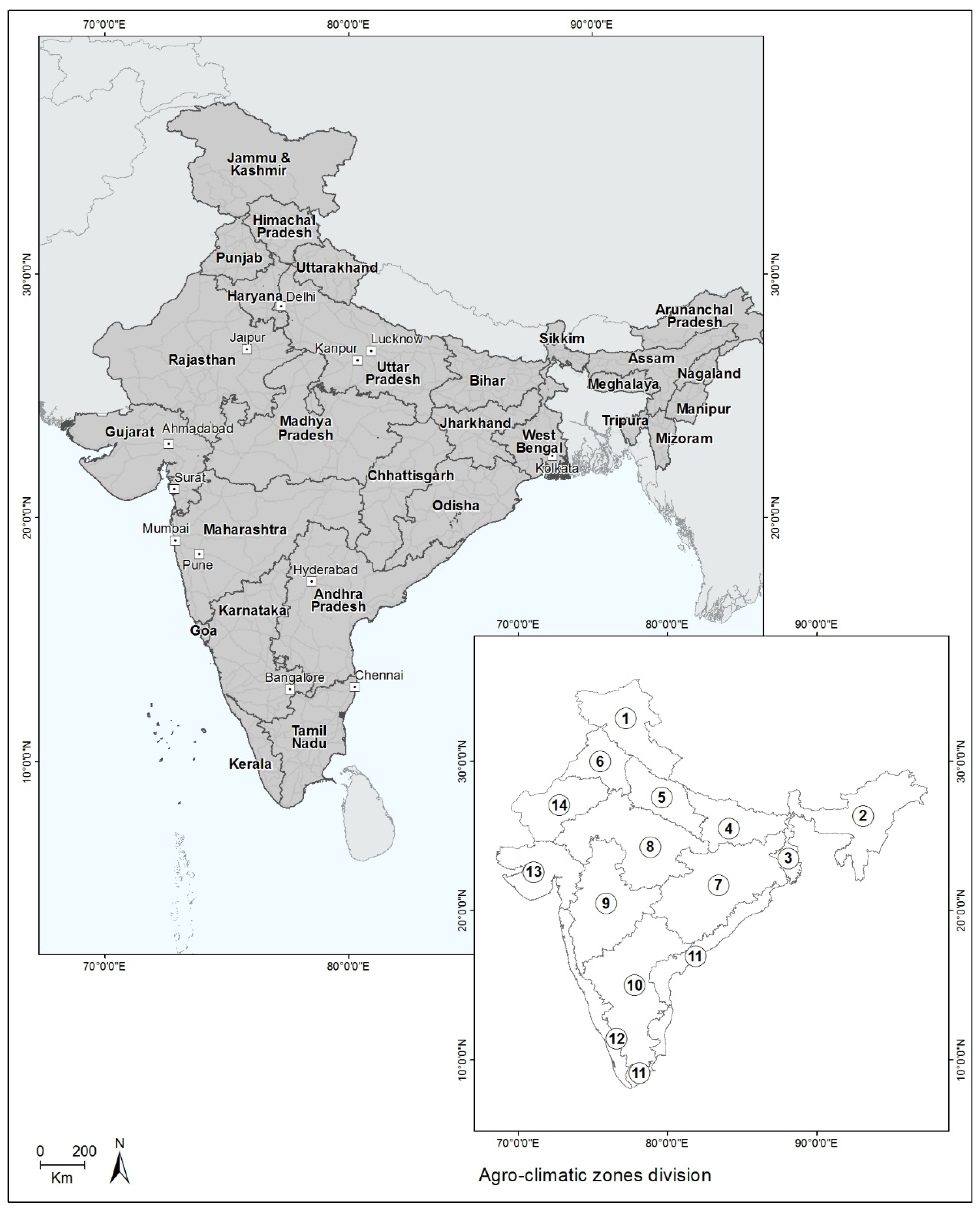
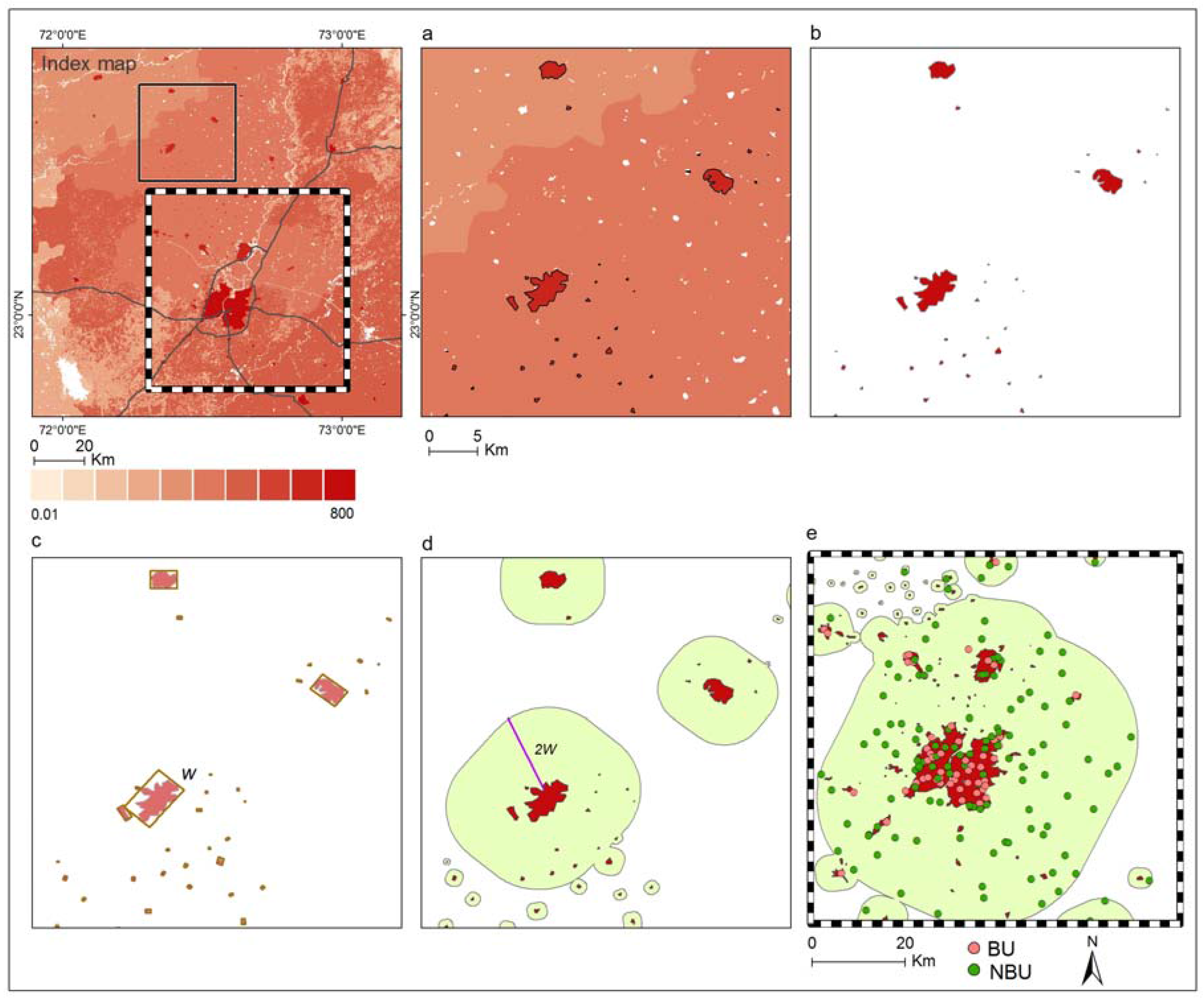
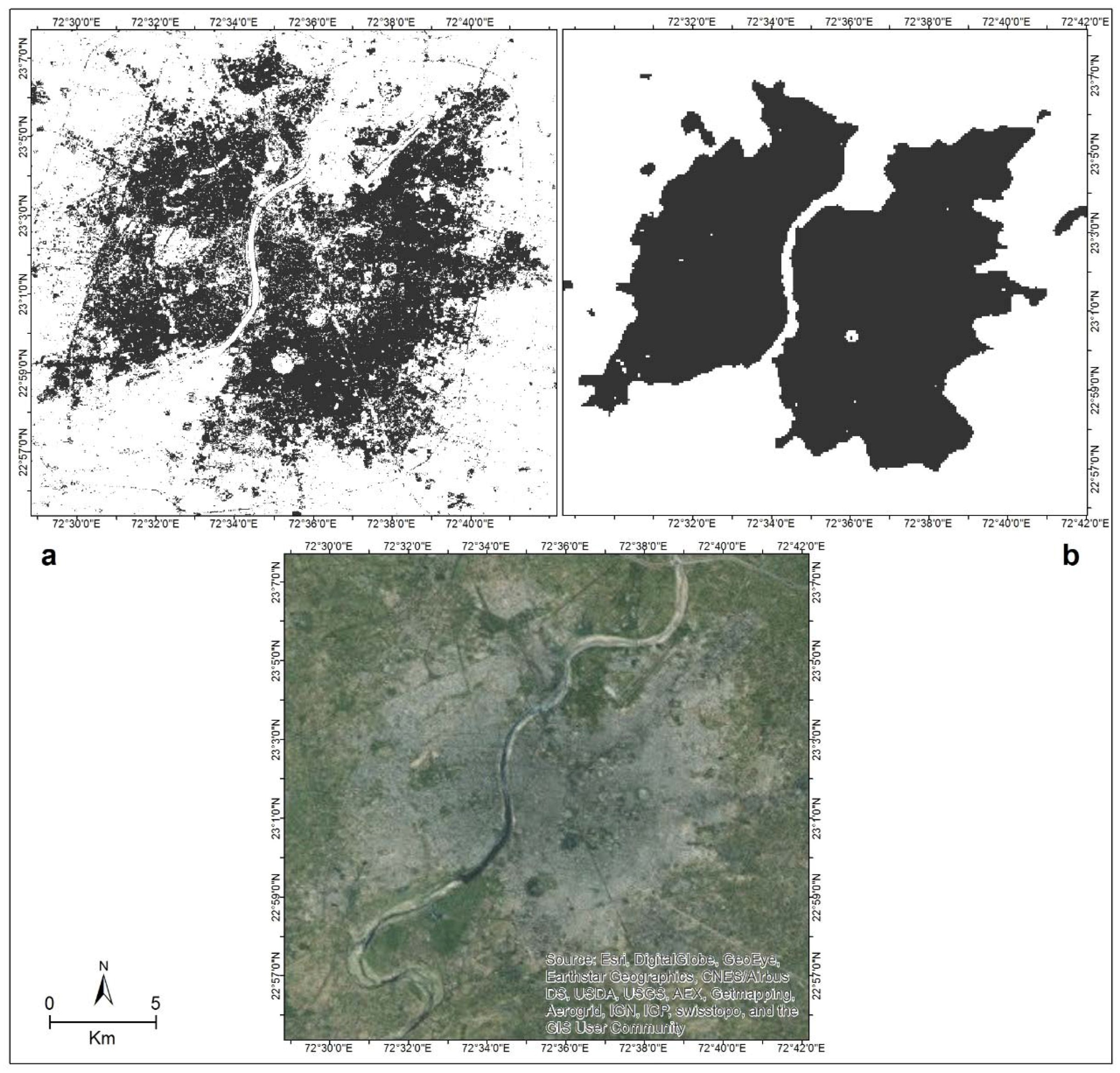
2.1. Study Area
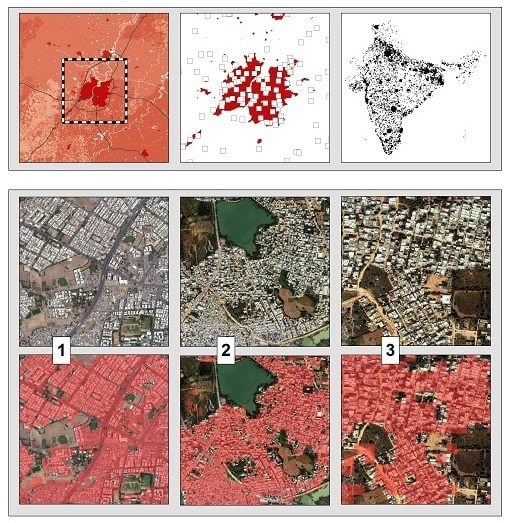
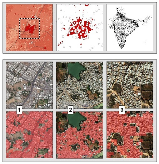
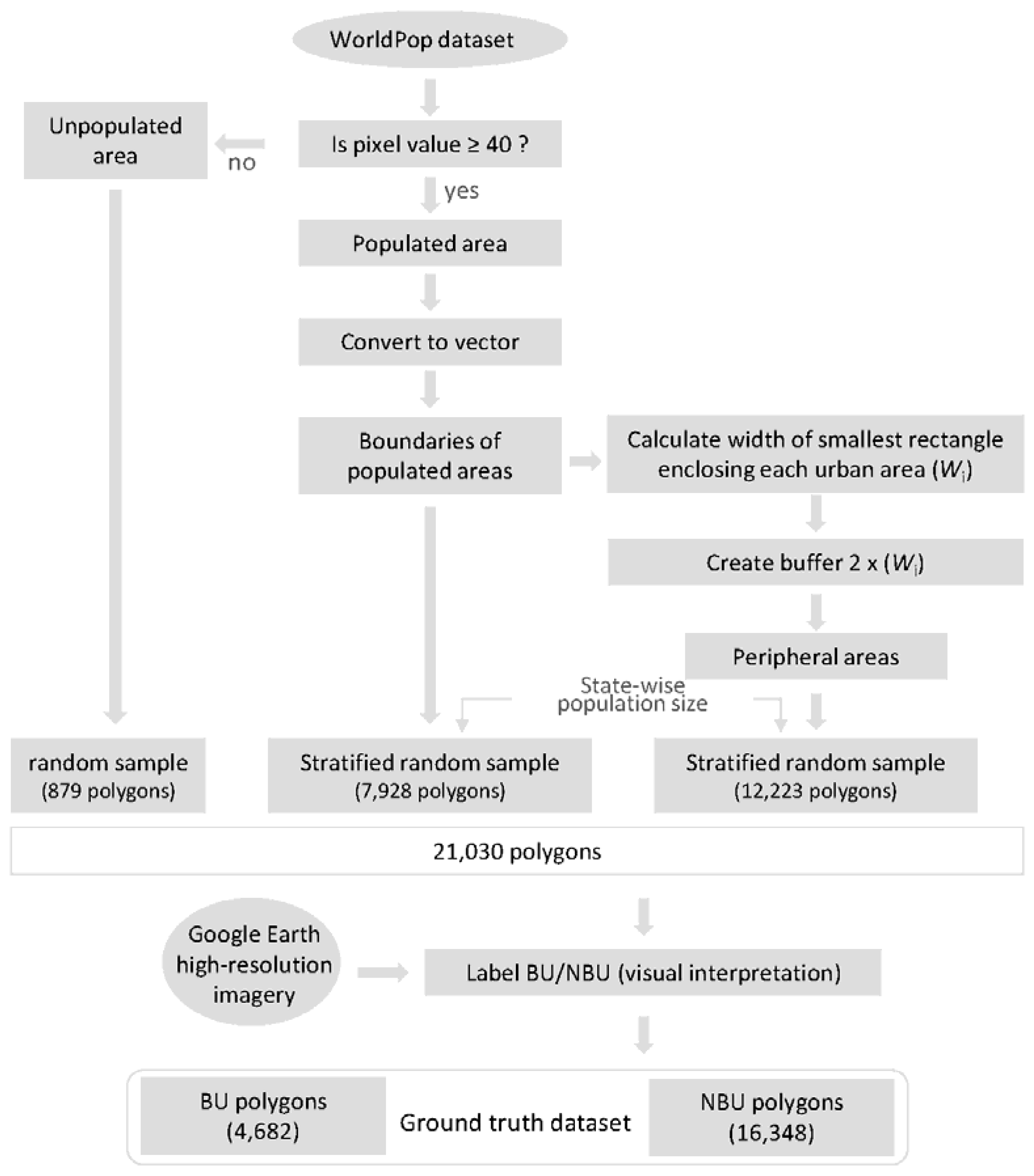
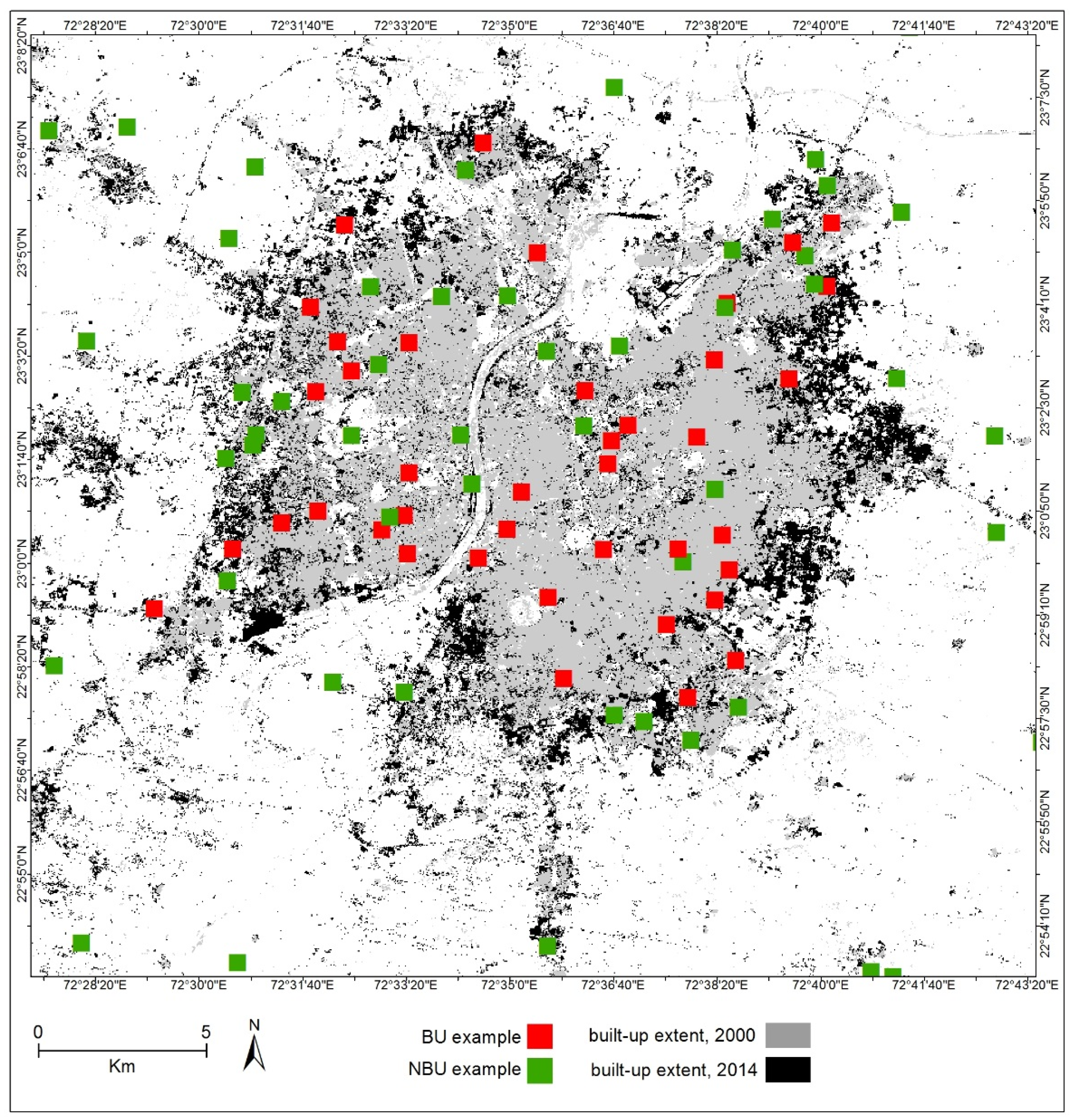
2.2. Dataset Construction
2.3. Pre-Processing and Scene Selection
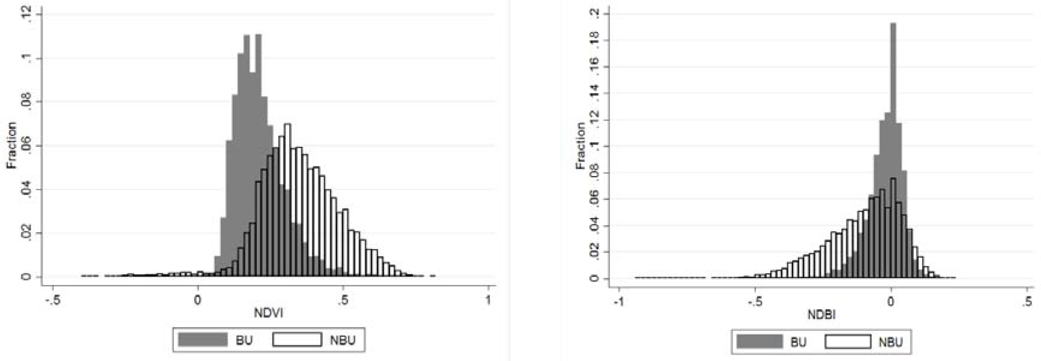
- NDVI expresses the relation between red visible light (which is typically absorbed by a plant’s chlorophyll) and near-infrared wavelength (which is scattered by the leaf’s mesophyll structure). It is computed as:where NIR is the near infra-red wavelength and RED is the red wavelength. The values of NDVI range between (−1) and (+1). An average NDVI value in 2014 was calculated for each pixel (with Landsat 7 32-Day NDVI Composite).(NIR − RED)/(NIR + RED)
- NDBI expresses the relation between the medium infra-red and the near infra-red wavelengths. It is computed as:where MIR is the medium infra-red and NIR is the near infra-red wavelength. The index assumes a higher reflectance of built-up areas in the medium infra-red wavelength range than in the near infra-red.(MIR − NIR)/(MIR + NIR)
2.4. Detection of Built-Up Areas
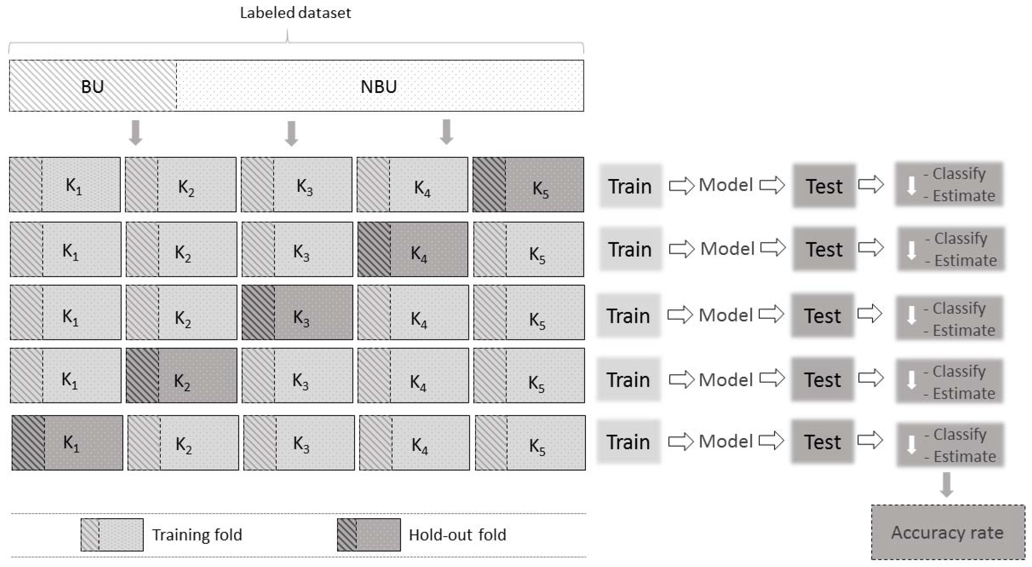
2.5. Accuracy Assessment
3. Results
3.1. Detection of Built-Up and Not Built-Up Areas
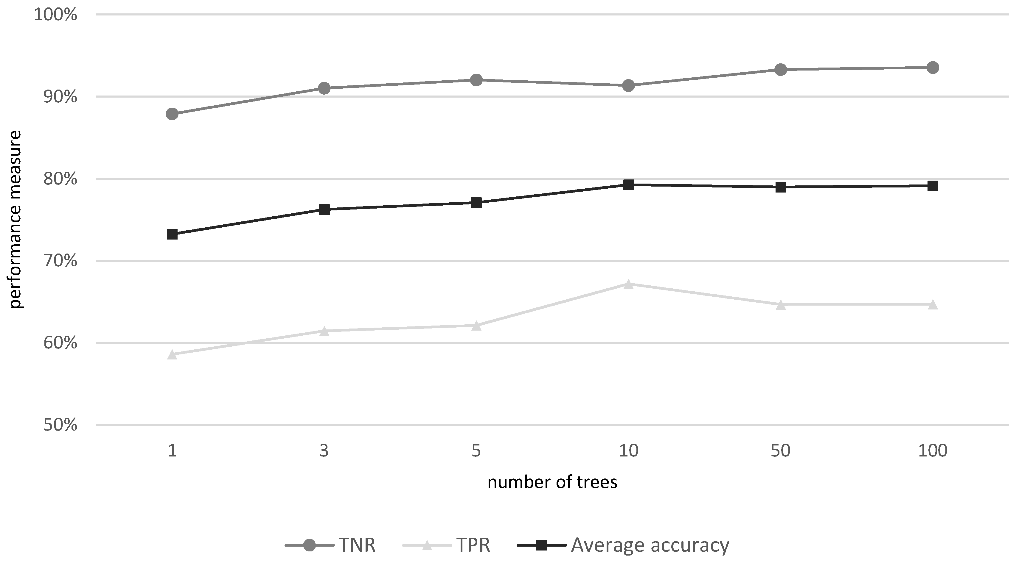
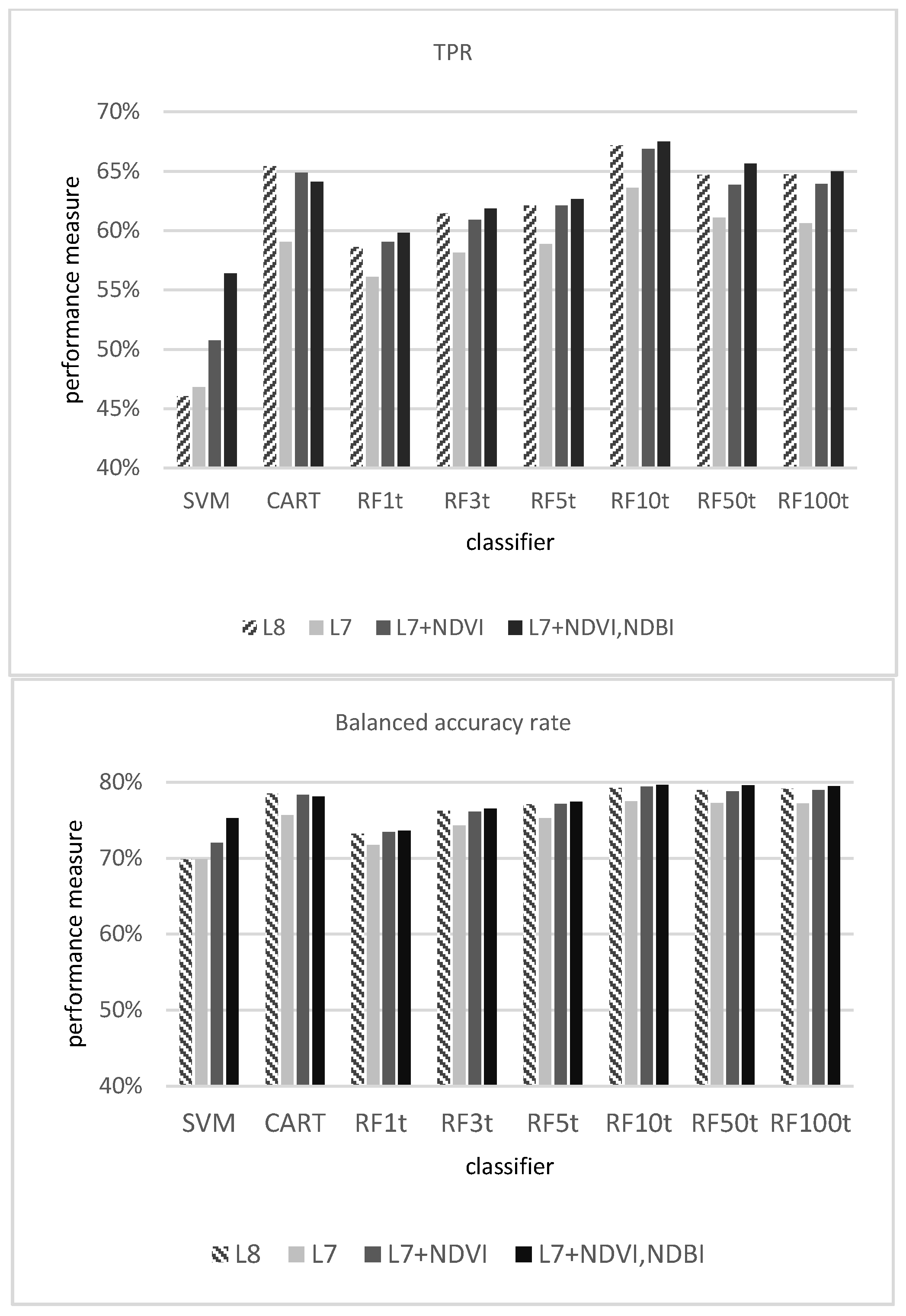
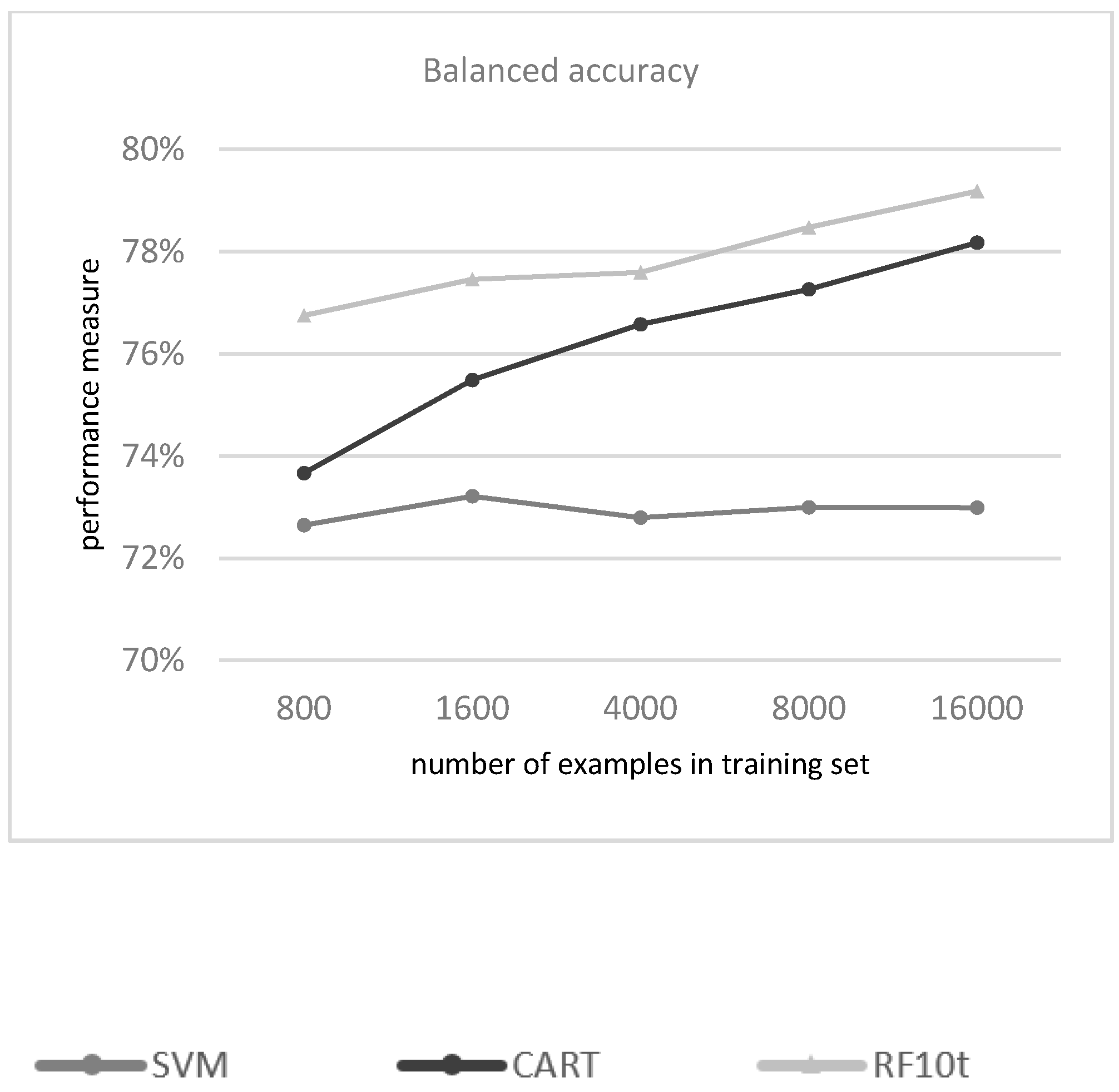
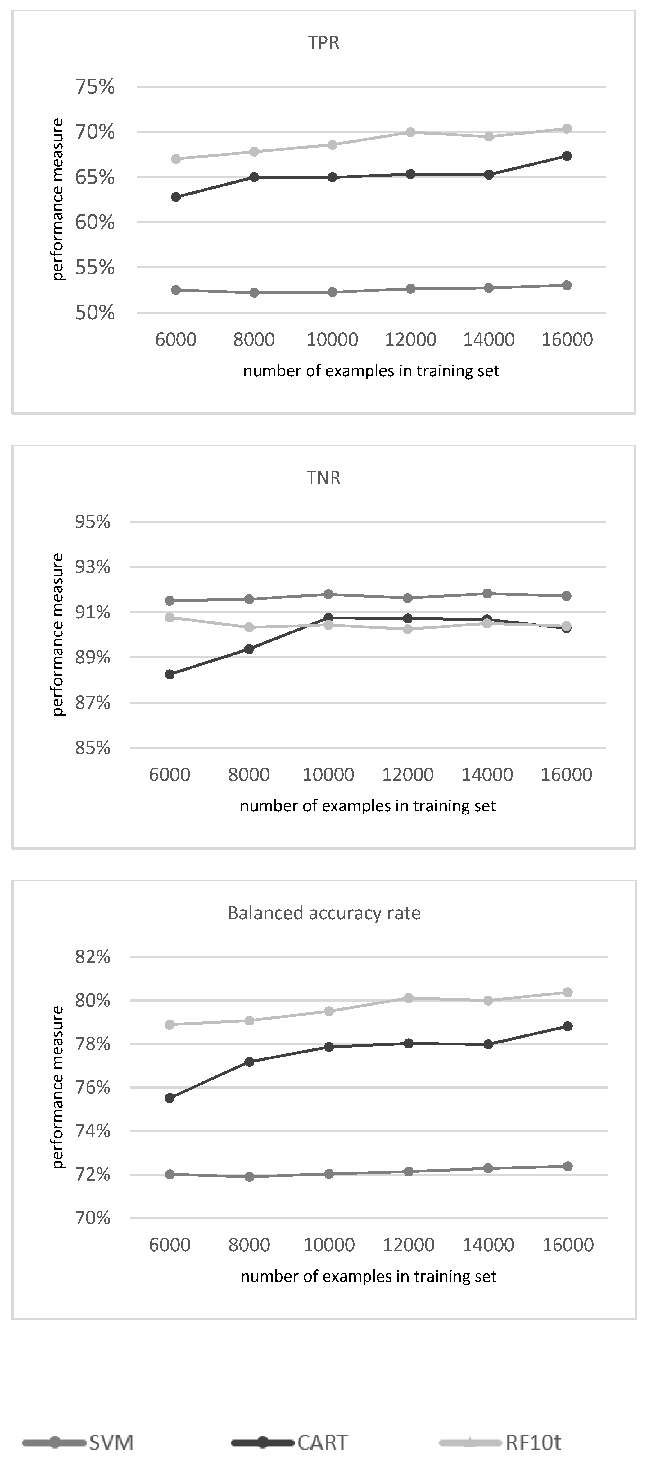
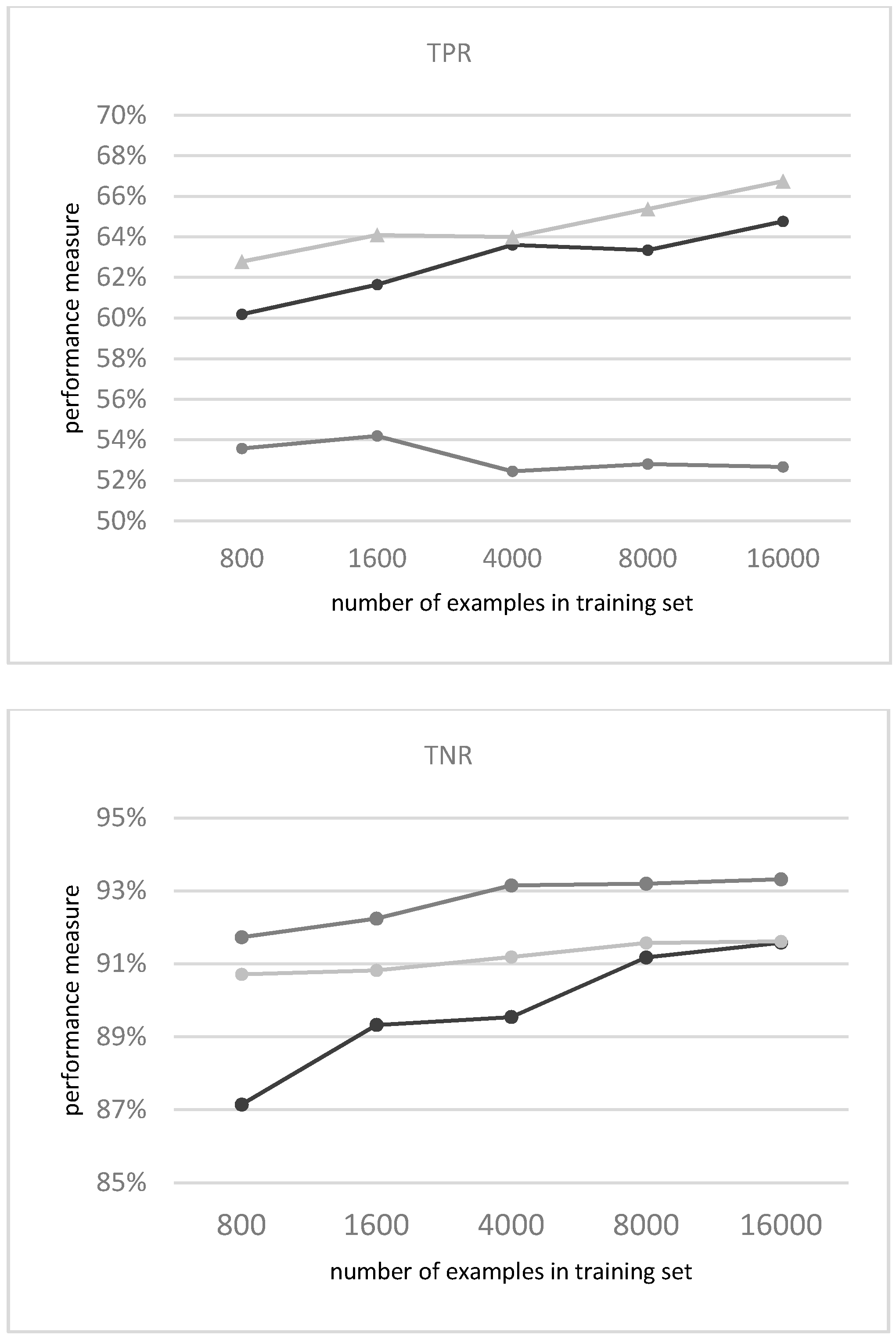
3.1.1. Evaluation of the Classifiers
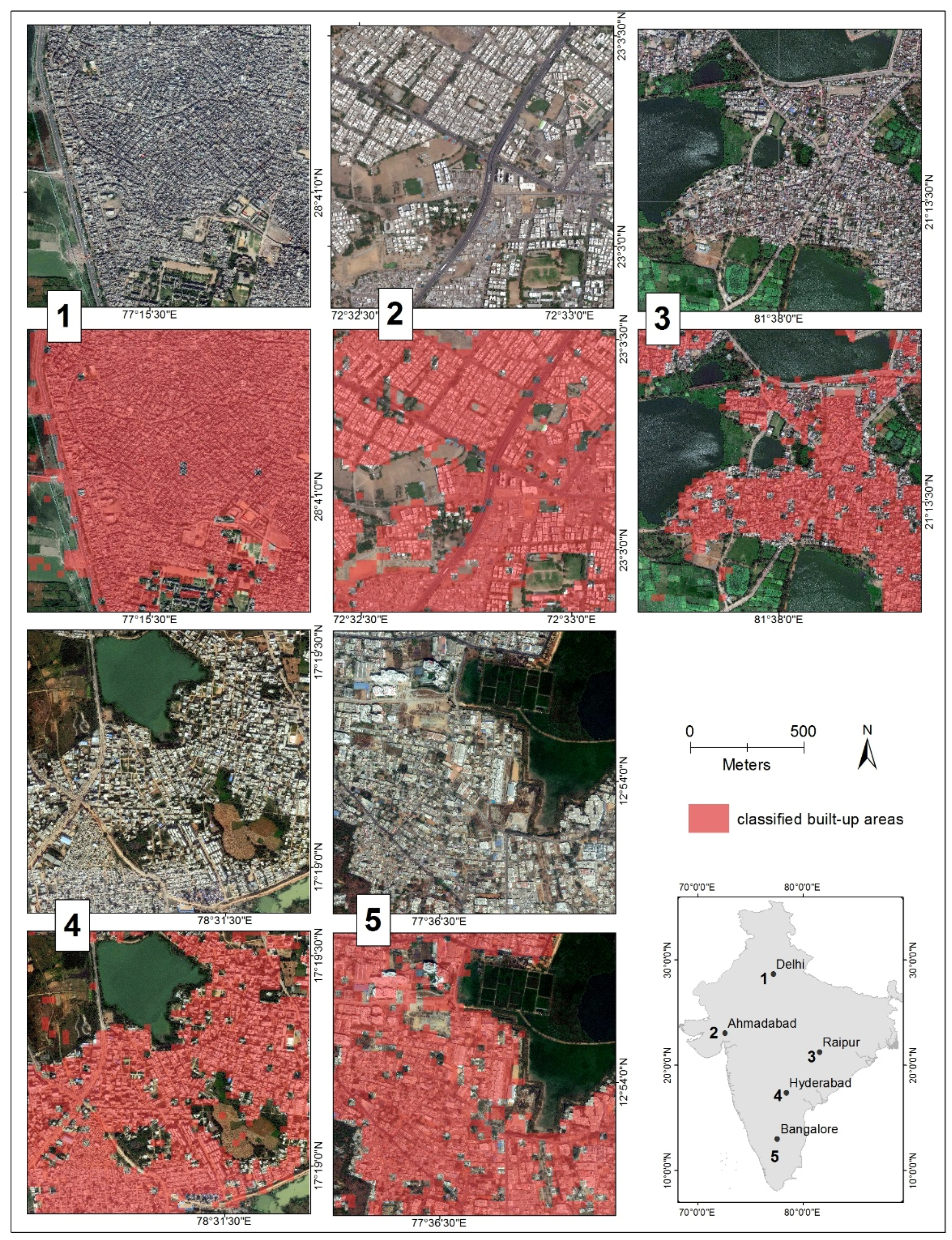
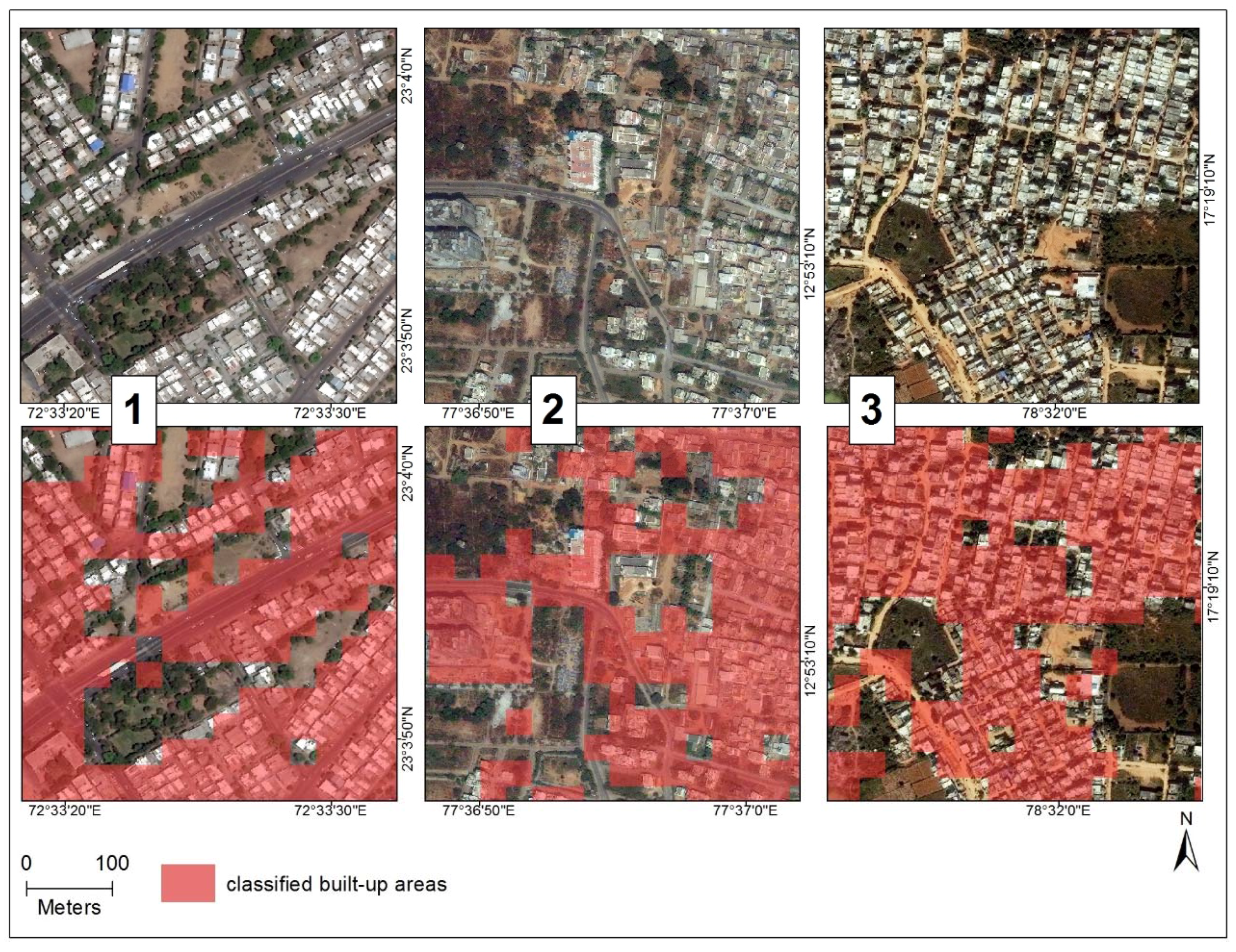
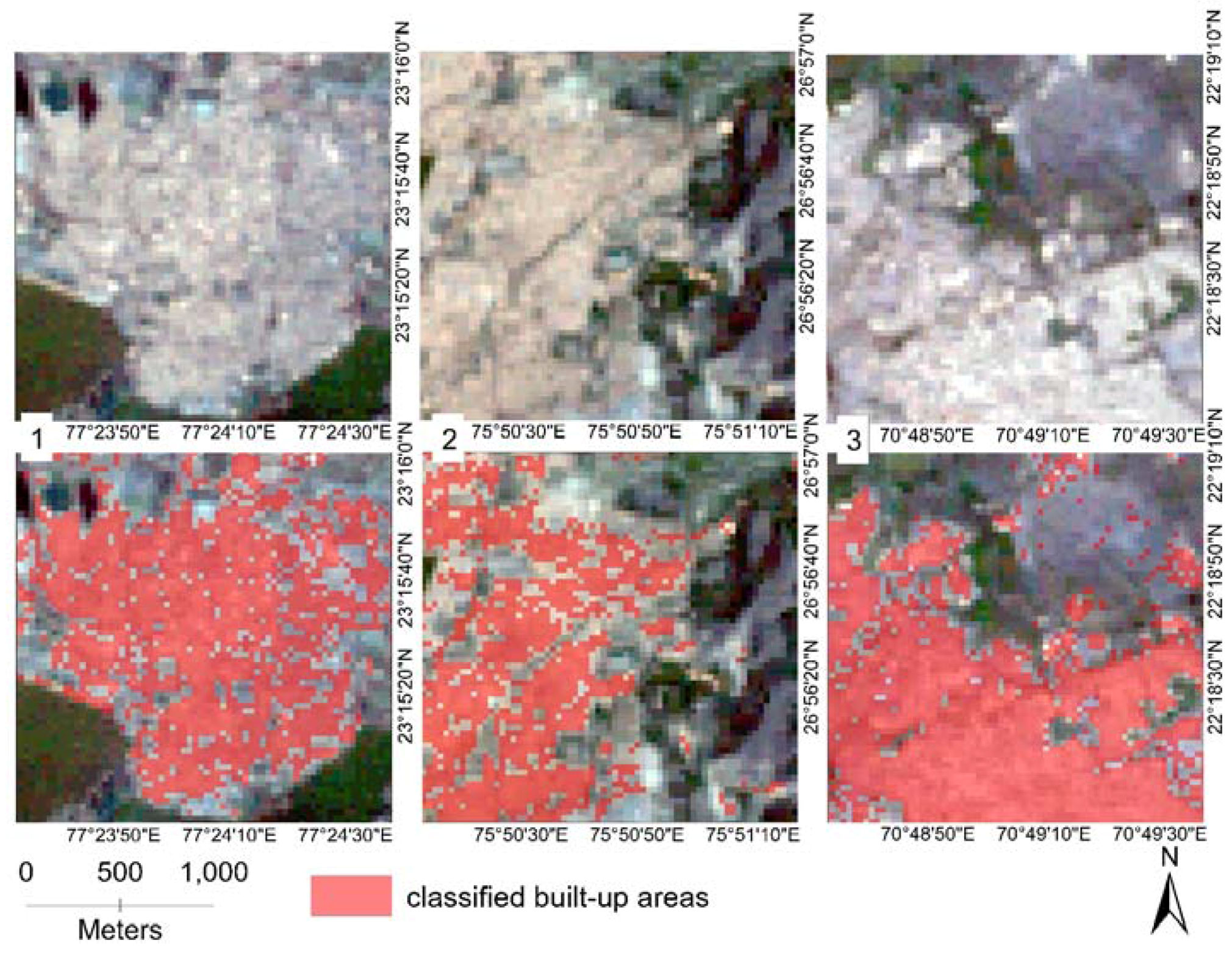
3.1.2. Mapping the Classification
4. Discussion
5. Conclusions
Author Contributions
Conflicts of Interest
Abbreviations
| GEE | Google Earth Engine |
| BU | built up |
| NBU | not built up |
| RF | Random forest |
| SVM | support vector machines |
| TPR | True Positive Rate |
| TNR | True Negative Rate |
Appendix A
- CART (Classification and Regression Tree) [35] is a binary decision tree. The classifier recursively examines each example’s variables with logical if-then questions in a binary tree structure. Questions are asked at each node of the tree, and each question typically looks at a single input variable. The variables are compared with a predetermined threshold, so that the examples are optimally split into “purer” subsets [35]. The examples are split to an overly large tree until reaching a terminal node (when the nodes have less than a defined number of examples or when further split will result in almost the same outcome). The tree is then pruned back through the creation of a nested sequence of less complex trees. The class is predicted at the terminal node according to the proportion of the classes in the training examples that reached that node.
- SVM (Support Vector Machines) identifies decision boundaries that optimally separate between classes. First, the n input vectors (examples) S = {X1,X2, … ,Xn} are mapped to the output classes by a linear decision function on a (possibly) high-dimensional feature space F = {φ(X1,X2, … ,Xn)}. SVM then optimizes the hyperplane that separates the classes by maximizing the margin between the support vectors of the classes (these are the examples that are closest to the decision surface) [37]. In this study we used a basic linear SVM.
- Random Forests are tree-based classifiers that include k decision trees (k predictors). When classifying an example, the example variables are run through each of the k tree predictors, and the k predictions are averaged to get a less noisy prediction (by voting on the most popular class). The learning process of the forest involves some level of randomness; each tree is trained over an independently random sample of examples from the training set and each node’s binary question in a tree is selected from a randomly sampled subset of the input variables [67].
Appendix B

| CART | |
| The cross-validation factor used for pruning | 10 |
| Maximal depth level of initial tree | 10 |
| Minimal number of training set points in node to allow node creation | 1 |
| Minimal number of points at node to allow its further split | 1 |
| The minimal cost of training set to allow split | 1e−10 |
| Whether to impose stopping criteria while growing the tree | false |
| The standard error threshold to use in determining the simplest tree whose accuracy is comparable to the minimum cost-complexity tree | 0.5 |
| The quantization resolution for numerical features | 100 |
| The margin reserved by quantizer to avoid overload, as a fraction of the range observed in the training data | 0.1 |
| The randomization seed | 0 |
| SVM | |
| The decision procedure to use | Voting |
| The SVM type | C_SVC |
| The kernel type | Linear |
| Whether to use shrinking heuristics | True |
| The cost (C) parameter | 1 |
| Random Forest | |
| The number of Rifle decision trees to create per class | 1,3,5,10,50,100 |
| The number of variables per split. If set to 0 (default), defaults to the square root of the number of variables | 0 |
| The minimum size of a terminal node | 1 |
| The fraction of input to bag per tree | 0.5 |
| Whether the classifier should run in out-of-bag mode | false |
References and Note
- Buhaug, H.; Urdal, H. An urbanization bomb? Population growth and social disorder in cities. Glob. Environ. Chang. 2013, 23, 1–10. [Google Scholar] [CrossRef]
- Glaeser, E.L. A world of cities: The causes and consequences of urbanization in poorer countries. J. Eur. Econ. Assoc. 2014, 12, 1154–1199. [Google Scholar] [CrossRef]
- Department of Economic and Social Affairs, Population Division, United Nations. World Urbanization Prospects: The 2014 Revision; United Nations: New York, NY, USA, 2015. [Google Scholar]
- Seto, K.C.; Güneralp, B.; Hutyra, L.R. Global forecasts of urban expansion to 2030 and direct impacts on biodiversity and carbon pools. Proc. Natl. Acad. Sci. USA 2012, 109, 16083–16088. [Google Scholar] [CrossRef] [PubMed]
- Wu, K.Y.; Ye, X.Y.; Qi, Z.F.; Zhang, H. Impacts of land use/land cover change and socioeconomic development on regional ecosystem services: The case of fast-growing Hangzhou metropolitan area, China. Cities 2013, 31, 276–284. [Google Scholar] [CrossRef]
- McKinney, M.L. Urbanization, Biodiversity, and Conservation: The impacts of urbanization on native species are poorly studied, but educating a highly urbanized human population about these impacts can greatly improve species conservation in all ecosystems. Bioscience 2002, 52, 883–890. [Google Scholar] [CrossRef]
- Pugh, C. Sustainability the Environment and Urbanisation; Earthscan: New York, NY, USA, 1996. [Google Scholar]
- Taubenböck, H.; Esch, T.; Felbier, A.; Wiesner, M.; Roth, A.; Dech, S. Monitoring urbanization in mega cities from space. Remote Sens. Environ. 2012, 117, 162–176. [Google Scholar] [CrossRef]
- Dewan, A.M.; Yamaguchi, Y. Land use and land cover change in Greater Dhaka, Bangladesh: Using remote sensing to promote sustainable urbanization. Appl. Geogr. 2009, 29, 390–401. [Google Scholar] [CrossRef]
- Bhatta, B. Analysis of urban growth pattern using remote sensing and GIS: A case study of Kolkata, India. Int. J. Remote Sens. 2009, 30, 4733–4746. [Google Scholar] [CrossRef]
- Gaughan, A.E.; Stevens, F.R.; Linard, C.; Jia, P.; Tatem, A.J. High resolution population distribution maps for Southeast Asia in 2010 and 2015. PLoS ONE 2013, 8, e55882. [Google Scholar] [CrossRef] [PubMed]
- Potere, D.; Schneider, A.; Angel, S.; Civco, D.L. Mapping urban areas on a global scale: Which of the eight maps now available is more accurate? Int. J. Remote Sens. 2009, 30, 6531–6558. [Google Scholar] [CrossRef]
- Schneider, A.; Friedl, M.A.; Potere, D. Mapping global urban areas using MODIS 500-m data: New methods and datasets based on ‘urban ecoregions’. Remote Sens. Environ. 2010, 114, 1733–1746. [Google Scholar] [CrossRef]
- Potere, D.; Schneider, A. Comparison of global urban maps. In Global Mapping of Human Settlement: Experiences, Datasets, and Prospects; Gamba, P., Herold, M., Eds.; CRC Press, Taylor and Francis Group: Boca Raton, FL, USA, 2009; pp. 269–309. [Google Scholar]
- Stevens, F.R.; Gaughan, A.E.; Linard, C.; Tatem, A.J. Disaggregating census data for population mapping using random forests with remotely-sensed and ancillary data. PLoS ONE 2015, 10, e0107042. [Google Scholar] [CrossRef] [PubMed]
- Belgiu, M.; Drǎguţ, L. Comparing supervised and unsupervised multiresolution segmentation approaches for extracting buildings from very high resolution imagery. ISPRS J. Photogramm. Remote Sens. 2014, 96, 67–75. [Google Scholar] [CrossRef] [PubMed]
- Estima, J.; Painho, M. Investigating the potential of OpenStreetMap for land use/land cover production: A case study for Continental Portugal. In OpenStreetMap in GIScience; Jokar Arsanjani, J., Zipf, A., Mooney, P., Helbich, M., Eds.; Springer International Publishing: Cham, Switzerland, 2015; pp. 273–293. [Google Scholar]
- Schlesinger, J. Using crowd-sourced data to quantify the complex urban fabric—OpenStreetMap and the urban–rural index. In OpenStreetMap in GIScience; Jokar Arsanjani, J., Zipf, A., Mooney, P., Helbich, M., Eds.; Springer International Publishing: Cham, Switzerland, 2015; pp. 295–315. [Google Scholar]
- Johnson, B.A.; Iizuka, K. Integrating OpenStreetMap crowdsourced data and Landsat time-series imagery for rapid land use/land cover (LULC) mapping: Case study of the Laguna de Bay area of the Philippines. Appl. Geogr. 2016, 67, 140–149. [Google Scholar] [CrossRef]
- Miyazaki, H.; Iwao, K.; Shibasaki, R. Development of a new ground truth database for global urban area mapping from a gazetteer. Remote Sens. 2011, 3, 1177–1187. [Google Scholar]
- The dataset can be accessed online as a Google Fusion Table at: https://www.google.com/fusiontables/DataSource?docid=1fWY4IyYiV-BA5HsAKi2V9LdoQgsbFtKK2BoQiHb0#rows:id=1 (Note: class “1” = “BU”, class “2” = “NBU”).
- Sudhira, H.S.; Ramachandra, T.V.; Jagadish, K.S. Urban sprawl: Metrics, dynamics and modelling using GIS. Int. J. Appl. Earth Obs. Geoinf. 2004, 5, 29–39. [Google Scholar] [CrossRef]
- Baum-Snow, N. Did highways cause suburbanization? Q. J. Econ. 2007, 122, 775–805. [Google Scholar] [CrossRef]
- Sudhira, H.S.; Ramachandra, T.V. Characterizing urban sprawl from remote sensing data and using landscape metrics. In Proceedings of the 10th International Conference on Computers in Urban Planning and Urban Management, Iguassu Falls, Brazil, 11–13 July 2007.
- Rahman, A.; Aggarwal, S.P.; Netzband, M.; Fazal, S. Monitoring urban sprawl using remote sensing and GIS techniques of a fast growing urban centre, India. IEEE J. Sel. Top. Appl. Earth Obs. Remote Sens. 2011, 4, 56–64. [Google Scholar] [CrossRef]
- Barnes, K.B.; Morgan, J.M., III; Roberge, M.C.; Lowe, S. Sprawl Devlopment: Its Patterns, Consequences, and Measurement; Towson University: Towson, MD, USA, 2001; pp. 1–24. [Google Scholar]
- Schneider, A. Monitoring land cover change in urban and peri-urban areas using dense time stacks of Landsat satellite data and a data mining approach. Remote Sens. Environ. 2012, 124, 689–704. [Google Scholar] [CrossRef]
- Bhatta, B.; Saraswati, S.; Bandyopadhyay, D. Urban sprawl measurement from remote sensing data. Appl. Geogr. 2010, 30, 731–740. [Google Scholar] [CrossRef]
- Jat, M.K.; Garg, P.K.; Khare, D. Monitoring and modelling of urban sprawl using remote sensing and GIS techniques. Int. J. Appl. Earth Obs. Geoinf. 2008, 10, 26–43. [Google Scholar] [CrossRef]
- Frenkel, A.; Ashkenazi, M. Measuring urban sprawl: How can we deal with it? Environ. Plan. B Plan. Des. 2008, 35, 56–79. [Google Scholar] [CrossRef]
- Yue, W.; Liu, Y.; Fan, P. Measuring urban sprawl and its drivers in large Chinese cities: The case of Hangzhou. Land Use Policy 2013, 31, 358–370. [Google Scholar] [CrossRef]
- Dahly, D.L.; Adair, L.S. Quantifying the urban environment: A scale measure of urbanicity outperforms the urban–rural dichotomy. Soc. Sci. Med. 2007, 64, 1407–1419. [Google Scholar] [CrossRef] [PubMed]
- Herold, M.; Goldstein, N.C.; Clarke, K.C. The spatiotemporal form of urban growth: Measurement, analysis and modeling. Remote Sens. Environ. 2003, 86, 286–302. [Google Scholar] [CrossRef]
- Small, C.; Pozzi, F.; Elvidge, C.D. Spatial analysis of global urban extent from DMSP-OLS night lights. Remote Sens. Environ. 2005, 96, 277–291. [Google Scholar] [CrossRef]
- Elvidge, C.D.; Safran, J.; Nelson, I.L.; Tuttle, B.T.; Hobson, V.R.; Baugh, K.E.; Dietz, J.; Erwin, W. Area and position accuracy of DMSP nighttime lights data. In Remote Sensing and GIS Accuracy Assessment; Lunetta, R.S., Lyon, J.G., Eds.; CRC Press: Boca Raton, FL, USA, 2004; pp. 281–292. [Google Scholar]
- Whiteside, T.; Ahmad, W. A comparison of object-oriented and pixel-based classification methods for mapping land cover in northern Australia. In Proceedings of the SSC2005 Spatial Intelligence, Innovation and Praxis: The National Biennial Conference of the Spatial Sciences Institute, Melbourne, Australia, 12–16 September 2005; pp. 1225–1231.
- Myint, S.W.; Gober, P.; Brazel, A.; Grossman-Clarke, S.; Weng, Q. Per-pixel vs. object-based classification of urban land cover extraction using high spatial resolution imagery. Remote Sens. Environ. 2011, 115, 1145–1161. [Google Scholar] [CrossRef]
- Whiteside, T.G.; Boggs, G.S.; Maier, S.W. Comparing object-based and pixel-based classifications for mapping savannas. Int. J. Appl. Earth Obs. Geoinf. 2011, 13, 884–893. [Google Scholar] [CrossRef]
- Bhaskaran, S.; Paramananda, S.; Ramnarayan, M. Per-pixel and object-oriented classification methods for mapping urban features using IKONOS satellite data. Appl. Geogr. 2010, 30, 650–665. [Google Scholar] [CrossRef]
- Duro, D.C.; Franklin, S.E.; Dubé, M.G. A comparison of pixel-based and object-based image analysis with selected machine learning algorithms for the classification of agricultural landscapes using SPOT-5 HRG imagery. Remote Sens. Environ. 2012, 118, 259–272. [Google Scholar] [CrossRef]
- Robertson, L.D.; King, D.J. Comparison of pixel-and object-based classification in land cover change mapping. Int. J. Remote Sens. 2011, 32, 1505–1529. [Google Scholar] [CrossRef]
- Breiman, L.; Friedman, J.H.; Stone, C.J.; Olshen, R.A. Classification and Regression Trees; Wadsworth: Belmont, CA, USA, 1984. [Google Scholar]
- Breiman, L. Random forests. Mach. Learn. 2001, 45, 5–32. [Google Scholar] [CrossRef]
- Cortes, C.; Vapnik, V. Support vector networks. Mach. Learn. 1995, 20, 273–297. [Google Scholar] [CrossRef]
- IASRI. Study Relating to Formulating Long Term Mechanization Strategy for Each Agro-Climatic Zone/State in India; Final report; Indian Agriculture Statistics Research Institute (IASRI): New Delhi, India, 2006. [Google Scholar]
- World Bank. Available online: http://data.worldbank.org/country/india (accessed on 20 March 2016).
- Census of India. Office of Registrar General & Census commissioner, Ministry of Home Affairs, Government of India. 2011. Available online: http://censusindia.gov.in/ (accessed on 15 May 2016). [Google Scholar]
- Chen, M.; Raveendran, G. Urban India 2011: Evidence; Indian Institute for Human Settlements Publications: Bangalore, India, 2011. [Google Scholar]
- Sudhira, H.S.; Gururaja, K.V. Population crunch in India: Is it urban or still rural? Curr. Sci. 2012, 103, 37–40. [Google Scholar]
- Prakasam, C. Land use and land cover change detection through remote sensing approach: A case study of Kodaikanal taluk, Tamil Nadu. Int. J. Geomat. Geosci. 2010, 1, 150–158. [Google Scholar]
- Moghadam, H.S.; Helbich, M. Spatiotemporal urbanization processes in the megacity of Mumbai, India: A Markov chains-cellular automata urban growth model. Appl. Geogr. 2013, 40, 140–149. [Google Scholar] [CrossRef]
- Ramachandra, T.V.; Aithal, B.H.; Sanna, D.D. Insights to urban dynamics through landscape spatial pattern analysis. Int. J. Appl. Earth Obs. Geoinf. 2012, 18, 329–343. [Google Scholar]
- Chadchan, J.; Shankar, R. An analysis of urban growth trends in the post-economic reforms period in India. Int. J. Sustain. Built Environ. 2012, 1, 36–49. [Google Scholar] [CrossRef]
- Sharma, R.; Joshi, P.K. Monitoring urban landscape dynamics over Delhi (India) using remote sensing (1998–2011) inputs. J. Indian Soc. Remote Sens. 2013, 41, 641–650. [Google Scholar] [CrossRef]
- Singh, P. Agro-Climatic Zonal Planning Including Agriculture Development in North Eastern India, for XI FIVE YEAR PLAN (2007–12); Planning Commission, Government of India: New Delhi, India, 2006.
- Palmer-Jones, R.; Sen, K. What has luck got to do with it? A regional analysis of poverty and agricultural growth in rural India. J. Dev. Stud. 2003, 40, 1–31. [Google Scholar] [CrossRef]
- Pettorelli, N.; Vik, J.O.; Mysterud, A.; Gaillard, J.-M.; Tucker, C.J.; Stenseth, N.C. Using the satellite-derived NDVI to assess ecological responses to environmental change. Trends Ecol. Evol. 2005, 20, 503–510. [Google Scholar] [CrossRef] [PubMed]
- Zha, Y.; Gao, J.; Ni, S. Use of normalized difference built-up index in automatically mapping urban areas from TM imagery. Int. J. Remote Sens. 2003, 24, 583–594. [Google Scholar] [CrossRef]
- Kohavi, R. A study of cross-validation and bootstrap for accuracy estimation and model selection. In Proceedings of the 14th International Joint Conference on Artificial Intelligence (IJCAI’95), Montreal, QC, Canada, 20–25 August 1995; Volume 2, pp. 1137–1143.
- Rodriguez, J.D.; Pérez, A.; Lozano, J.A. Sensitivity analysis of k-fold cross validation in prediction error estimation. IEEE Trans. Pattern Anal. Mach. Intell. 2010, 32, 569–575. [Google Scholar] [CrossRef] [PubMed]
- Salzberg, S.L. On comparing classifiers: Pitfalls to avoid and a recommended approach. Data Min. Knowl. Discov. 1997, 1, 317–328. [Google Scholar] [CrossRef]
- Arlot, S.; Celisse, A. A survey of cross-validation procedures for model selection. Stat. Surv. 2010, 4, 40–79. [Google Scholar] [CrossRef]
- Refaeilzadeh, P.; Tang, L.; Liu, H. Cross-validation. In Encyclopedia of Database Systems; Liu, L., Özsu, M.T., Eds.; Springer US: New York, NY, USA, 2009; pp. 532–538. [Google Scholar]
- Blum, A.; Kalai, A.; Langford, J. Beating the hold-out: Bounds for k-fold and progressive cross-validation. In Proceedings of the 12th Annual Conference on Computational Learning Theory, Santa Cruz, CA, USA, 7–9 July 1999; pp. 203–208.
- Bradford, J.P.; Brodley, C.E. The effect of instance-space partition on significance. Mach. Learn. 2001, 42, 269–286. [Google Scholar] [CrossRef]
- Rodriguez-Galiano, V.F.; Ghimire, B.; Rogan, J.; Chica-Olmo, M.; Rigol-Sanchez, J.P. An assessment of the effectiveness of a random forest classifier for land-cover classification. ISPRS J. Photogramm. Remote Sens. 2012, 67, 93–104. [Google Scholar] [CrossRef]
- Tatem, A.J.; Noor, A.M.; Von Hagen, C.; Di Gregorio, A.; Hay, S.I. High resolution population maps for low income nations: Combining land cover and census in East Africa. PLoS ONE 2007, 2, e1298. [Google Scholar] [CrossRef] [PubMed]
- Orenstein, D.; Bradley, B.; Albert, J.; Mustard, J.; Hamburg, S. How much is built? Quantifying and interpreting patterns of built space from different data sources. Int. J. Remote Sens. 2011, 32, 2621–2644. [Google Scholar] [CrossRef]
- CIESIN, Columbia University. Gridded Population of the World, Version 3 (GPWv3) Data Collection. Available online: http://sedac.ciesin.columbia.edu/data/collection/gpw-v3 (accessed on 2 April 2016).
- Patel, N.N.; Angiuli, E.; Gamba, P.; Gaughan, A.; Lisini, G.; Stevens, F.R.; Tatem, A.J.; Trianni, G. Multitemporal settlement and population mapping from Landsat using Google Earth Engine. Int. J. Appl. Earth Obs. Geoinf. 2015, 35, 199–208. [Google Scholar] [CrossRef]
- Gislason, P.O.; Benediktsson, J.A.; Sveinsson, J.R. Random forests for land cover classification. Pattern Recognit. Lett. 2006, 27, 294–300. [Google Scholar] [CrossRef]
- Shao, Y.; Lunetta, R.S. Comparison of support vector machine, neural network, and CART algorithms for the land-cover classification using limited training data points. ISPRS J. Photogramm. Remote Sens. 2012, 70, 78–87. [Google Scholar] [CrossRef]
- Wieland, M.; Pittore, M. Performance evaluation of machine learning algorithms for urban pattern recognition from multi-spectral satellite images. Remote Sens. 2014, 6, 2912–2939. [Google Scholar] [CrossRef]
- Xie, M.; Jean, N.; Burke, M.; Lobell, D.; Ermon, S. Transfer learning from deep features for remote sensing and poverty mapping. arXiv Preprint, 2015; arXiv:1510.00098. [Google Scholar]
- Trianni, G.; Lisini, G.; Angiuli, E.; Moreno, E.A.; Dondi, P.; Gaggia, A.; Gamba, P. Scaling up to national/regional urban extent mapping using Landsat data. IEEE J. Sel. Top. Appl. Earth Obs. Remote Sens. 2015, 8, 3710–3719. [Google Scholar] [CrossRef]
- Hansen, M.C.; Potapov, P.V.; Moore, R.; Hancher, M.; Turubanova, S.A.; Tyukavina, A.; Thau, D.; Stehman, S.V.; Goetz, S.J.; Loveland, T.R.; Kommareddy, A. High-resolution global maps of 21st-century forest cover change. Science 2013, 342, 850–853. [Google Scholar] [CrossRef] [PubMed]
- Qian, Y.; Zhou, W.; Yan, J.; Li, W.; Han, L. Comparing machine learning classifiers for object-based land cover classification using very high resolution imagery. Remote Sens. 2015, 7, 153–168. [Google Scholar] [CrossRef]


| Spectral Band | Wavelength (Micrometers) | Resolution (Meters) | |
|---|---|---|---|
| Landsat 7 | |||
| B1 | Band 1—blue-green | 0.45–0.52 | 30 |
| B2 | Band 2—green | 0.52–0.61 | 30 |
| B3 | Band 3—red | 0.63–0.69 | 30 |
| B4 | Band 4—reflected IR | 0.76–0.90 | 30 |
| B5 | Band 5—reflected IR | 1.55–1.75 | 30 |
| B6 | Band 6—thermal | 10.40–12.50 | 120 |
| B7 | Band 7—reflected IR | 2.08–2.35 | 30 |
| NDVI | (B4 − B3)/(B4 + B3) | 30 | |
| NDBI | (B5 − B4)/(B5 + B4) | 30 | |
| Landsat 8 | |||
| B1 | Band 1—Ultra blue | 0.43–0.45 | 30 |
| B2 | Band 2—Blue | 0.45–0.51 | 30 |
| B3 | Band 3—Green | 0.53–0.59 | 30 |
| B4 | Band 4—Red | 0.64–0.67 | 30 |
| B5 | Band 5—Near Infrared (NIR) | 0.85–0.88 | 30 |
| B6 | Band 6—SWIR 1 | 1.57–1.65 | 30 |
| B7 | Band 7—SWIR 2 | 2.11–2.29 | 30 |
| B8 | Band 8—Panchromatic | 0.50–0.68 | 15 |
| B10 | Band 10—Thermal Infrared (TIRS) 1 | 10.60–11.19 | 100 (resampled to 30) |
| B11 | Band 11—Thermal Infrared (TIRS) 2 | 11.50–12.51 | 100 (resampled to 30) |
| Zone Number | Number of Examples | BU/NBU Ratio | ||
|---|---|---|---|---|
| BU | NBU | BU | NBU | |
| 1 | 82 | 476 | 14.7% | 85.3% |
| 2 | 169 | 825 | 17.0% | 83.0% |
| 3 | 222 | 837 | 21.0% | 79.0% |
| 4 | 425 | 1816 | 19.0% | 81.0% |
| 5 | 671 | 2024 | 24.9% | 75.1% |
| 6 | 382 | 953 | 28.6% | 71.4% |
| 7 | 326 | 1545 | 17.4% | 82.6% |
| 8 | 333 | 1066 | 23.8% | 76.2% |
| 9 | 421 | 1464 | 22.3% | 77.7% |
| 10 | 645 | 1979 | 24.6% | 75.4% |
| 11 | 391 | 1197 | 24.6% | 75.4% |
| 12 | 250 | 894 | 21.9% | 78.1% |
| 13 | 262 | 805 | 24.6% | 75.4% |
| 14 | 103 | 467 | 18.1% | 81.9% |
| Total | 4682 | 16,348 | ||
| B1 | B2 | B3 | B4 | B5 | B6 | B7 | B8 | NDVI | NDBI | ||
|---|---|---|---|---|---|---|---|---|---|---|---|
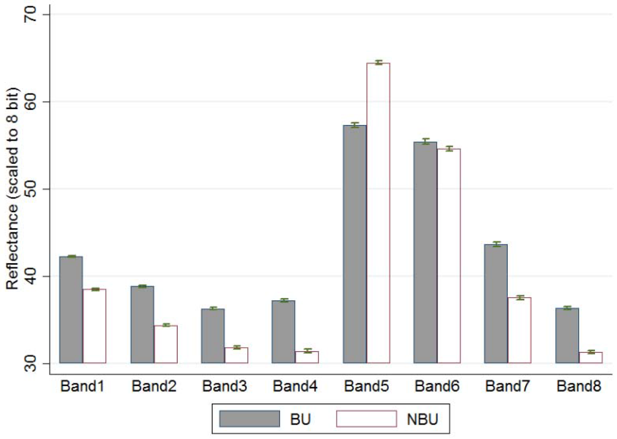
| BU | (mean) | 42.27 | 38.84 | 36.29 | 37.20 | 57.29 | 55.44 | 43.64 | 36.36 | 0.21 | −0.02 |
| (st. err.) | 0.048 | 0.058 | 0.073 | 0.099 | 0.126 | 0.151 | 0.137 | 0.085 | 0.001 | 0.001 | |
| NBU | (mean) | 38.51 | 34.37 | 31.82 | 31.43 | 64.49 | 54.65 | 37.54 | 31.27 | 0.35 | −0.10 |
| (st. err.) | 0.069 | 0.075 | 0.081 | 0.097 | 0.104 | 0.132 | 0.120 | 0.087 | 0.001 | 0.001 | |
| t-tests of equal means | (t-stats) | 44.91 | 47.17 | 40.95 | 41.50 | −43.99 | 3.92 | 33.54 | 41.92 | −85.98 | 57.02 |
| (p-value) | 0.000 | 0.000 | 0.000 | 0.000 | 0.000 | 0.000 | 0.000 | 0.000 | 0.000 | 0.000 | |
| K-S tests of equal dist * | (p-value) | 0.000 | 0.000 | 0.000 | 0.000 | 0.000 | 0.000 | 0.000 | 0.000 | 0.000 | 0.000 |
| Predicted | |||||||||||
|---|---|---|---|---|---|---|---|---|---|---|---|
| L8 | L7 | L7 + NDVI + NDBI | |||||||||
| BU | NBU | Total | BU | NBU | Total | BU | NBU | Total | |||
| Actual | SVM | BU | 2347 | 2750 | 5097 | 2376 | 2700 | 5076 | 2863 | 2213 | 5076 |
| NBU | 1122 | 16727 | 17849 | 1261 | 16659 | 17920 | 1044 | 16876 | 17920 | ||
| Total | 3469 | 19477 | 22946 | 3637 | 19359 | 22996 | 3907 | 19089 | 22996 | ||
| Ac: 0.831 Re: 0.460 Pre: 0.677 | Ac: 0.828 Re: 0.468 Pre: 0.653 | Ac: 0.858 Re: 0.564 Pre: 0.733 | |||||||||
| CART | BU | 3335 | 1762 | 5097 | 2998 | 2078 | 5076 | 3253 | 1823 | 5076 | |
| NBU | 1500 | 16349 | 17849 | 1380 | 16540 | 17920 | 1413 | 16507 | 17920 | ||
| Total | 4835 | 18111 | 22946 | 4378 | 18618 | 22996 | 4666 | 18330 | 22996 | ||
| Ac: 0.858 Re: 0.654 Pre: 0.690 | Ac: 0.850 Re: 0.591 Pre: 0.685 | Ac: 0.859 Re: 0.641 Pre: 0.697 | |||||||||
| RF3t | BU | 3133 | 1964 | 5097 | 2951 | 2125 | 5076 | 3140 | 1936 | 5076 | |
| NBU | 1601 | 16248 | 17849 | 1709 | 16211 | 17920 | 1576 | 16344 | 17920 | ||
| Total | 4734 | 18212 | 22946 | 4660 | 18336 | 22996 | 4716 | 18280 | 22996 | ||
| Ac: 0.845 Re: 0.615 Pre: 0.662 | Ac: 0.833 Re: 0.581 Pre: 0.633 | Ac: 0.847 Re: 0.619 Pre: 0.666 | |||||||||
| RF5t | BU | 3167 | 1930 | 5097 | 2989 | 2087 | 5076 | 3181 | 1895 | 5076 | |
| NBU | 1423 | 16426 | 17849 | 1494 | 16426 | 17920 | 1402 | 16518 | 17920 | ||
| Total | 4590 | 18356 | 22946 | 4483 | 18513 | 22996 | 4583 | 18413 | 22996 | ||
| Ac: 0.854 Re: 0.621 Pre: 0.690 | Ac: 0.844 Re: 0.589 Pre: 0.667 | Ac: 0.857 Re: 0.627 Pre: 0.694 | |||||||||
| RF10t | BU | 3424 | 1673 | 5097 | 3229 | 1847 | 5076 | 3426 | 1650 | 5076 | |
| NBU | 1543 | 16306 | 17849 | 1539 | 16381 | 17920 | 1471 | 16449 | 17920 | ||
| Total | 4967 | 17979 | 22946 | 4768 | 18228 | 22996 | 4897 | 18099 | 22996 | ||
| Ac: 0.860 Re: 0.672 Pre: 0.689 | Ac: 0.853 Re: 0.636 Pre: 0.677 | Ac: 0.864 Re: 0.675 Pre: 0.700 | |||||||||
| RF50t | BU | 3297 | 1800 | 5097 | 3102 | 1974 | 5076 | 3332 | 1744 | 5076 | |
| NBU | 1196 | 16653 | 17849 | 1180 | 16740 | 17920 | 1153 | 16767 | 17920 | ||
| Total | 4493 | 18453 | 22946 | 4282 | 18714 | 22996 | 4485 | 18511 | 22996 | ||
| Ac: 0.869 Re: 0.647 Pre: 0.734 | Ac: 0.863 Re: 0.611 Pre: 0.724 | Ac: 0.874 Re: 0.656 Pre: 0.743 | |||||||||
| RF100t | BU | 3299 | 1798 | 5097 | 3078 | 1998 | 5076 | 3299 | 1777 | 5076 | |
| NBU | 1151 | 16698 | 17849 | 1116 | 16804 | 17920 | 1088 | 16832 | 17920 | ||
| Total | 4450 | 18496 | 22946 | 4194 | 18802 | 22996 | 4387 | 18609 | 22996 | ||
| Ac: 0.871 Re: 0.647 Pre: 0.741 | Ac: 0.865 Re: 0.606 Pre: 0.734 | Ac: 0.875 Re: 0.650 Pre:0.752 | |||||||||
| Predicted | ||||
|---|---|---|---|---|
| BU | NBU | Total | ||
| Actual | BU | 34 | 24 | 58 |
| NBU | 4 | 138 | 142 | |
| Total | 38 | 162 | 200 | |
© 2016 by the authors; licensee MDPI, Basel, Switzerland. This article is an open access article distributed under the terms and conditions of the Creative Commons Attribution (CC-BY) license (http://creativecommons.org/licenses/by/4.0/).
Share and Cite
Goldblatt, R.; You, W.; Hanson, G.; Khandelwal, A.K. Detecting the Boundaries of Urban Areas in India: A Dataset for Pixel-Based Image Classification in Google Earth Engine. Remote Sens. 2016, 8, 634. https://doi.org/10.3390/rs8080634
Goldblatt R, You W, Hanson G, Khandelwal AK. Detecting the Boundaries of Urban Areas in India: A Dataset for Pixel-Based Image Classification in Google Earth Engine. Remote Sensing. 2016; 8(8):634. https://doi.org/10.3390/rs8080634
Chicago/Turabian StyleGoldblatt, Ran, Wei You, Gordon Hanson, and Amit K. Khandelwal. 2016. "Detecting the Boundaries of Urban Areas in India: A Dataset for Pixel-Based Image Classification in Google Earth Engine" Remote Sensing 8, no. 8: 634. https://doi.org/10.3390/rs8080634
APA StyleGoldblatt, R., You, W., Hanson, G., & Khandelwal, A. K. (2016). Detecting the Boundaries of Urban Areas in India: A Dataset for Pixel-Based Image Classification in Google Earth Engine. Remote Sensing, 8(8), 634. https://doi.org/10.3390/rs8080634