Predicting Grassland Leaf Area Index in the Meadow Steppes of Northern China: A Comparative Study of Regression Approaches and Hybrid Geostatistical Methods

Abstract

Leaf area index (LAI) is a key parameter used to describe vegetation structures and is widely used in ecosystem biophysical process and vegetation productivity models. Many algorithms have been developed for the estimation of LAI based on remote sensing images. Our goal was to produce accurate and timely predictions of grassland LAI for the meadow steppes of northern China. Here, we compare the predictive power of regression approaches and hybrid geostatistical methods using Chinese Huanjing (HJ) satellite charge coupled device (CCD) data. The regression methods evaluated include partial least squares regression (PLSR), artificial neural networks (ANNs) and random forests (RFs). The two hybrid geostatistical methods were regression kriging (RK) and random forests residuals kriging (RFRK). The predictions were validated for different grassland types and different growing stages, and their performances were also examined by adding several groups of vegetation indices (VIs). The two hybrid geostatistical models (RK and RFRK) yielded the most accurate predictions (root mean squared error (RMSE) = 0.21 m²/m² and 0.23 m²/m² for RK and RFRK, respectively), followed by the RF model (RMSE = 0.27 m²/m²), which was the most accurate among the regression models. These three models also exhibited the best temporal performance across the duration of the growing season. The PLSR and ANN models were less accurate (RMSE = 0.33 m²/m² and 0.35 m²/m² for ANN and PLSR, respectively), and the PLSR model performed the worst (exhibiting varied temporal performance and unreliable prediction accuracy that was susceptible to ground conditions). By adding VIs to the predictor variables, the predictions of the PLSR and ANN models were obviously improved (RMSE improved from 0.35 m²/m² to 0.28 m²/m² for PLSR and from 0.33 m²/m² to 0.28 m²/m² for ANN); the RF and RFRK models did not generate more accurate predictions and the performance of the RK model declined (RMSE decreased from 0.21 m²/m² to 0.32 m²/m²).

1. Introduction

Leaf area index (LAI) is defined as the one-sided green leaf area per unit ground area [1] and is a crucial parameter driving the biological processes of plants. The index is closely associated with vegetative biological and physical processes, such as photosynthesis and transpiration. Therefore, LAI is used as an essential input in a variety of climate and ecosystem models [2,3,4,5]. As an important indicator describing the energy and carbon exchange between vegetation and the atmosphere, the quantitative retrieval of this biophysical parameter is necessary for understanding the changes in energy and carbon cycling in response to climate change [5,6,7].

To this end, remote sensing data, which are endowed with high temporal resolution and the capacity for large-scale observation, are widely used for LAI prediction. A number of LAI prediction methods have been developed from remotely sensed data. The most popular and commonly used approaches are empirical statistical methods, including simple linear regression [8], multiple linear regression [9], and partial least squares regression (PLSR) [10]. These methods primarily compute the relationship between LAI and a spectral observation or a combination of spectral observations (vegetation indices, VIs) by relying on statistical or physical knowledge. However, due to their empirical nature, these regression models are site and sensor specific, and their performance can be hampered by factors, such as differences in surface properties and sun position, as well as viewing geometry [11,12,13]. Machine learning methods, such as decision tree learning, artificial neural networks (ANNs) [14], support vector machines [15], and random forests (RFs) [16,17] are also increasingly employed to optimize the use of spectral information with the goal of minimizing prediction uncertainty. The non-linear relationship between remote sensing data and biogeophysical variables endows these flexible models with the ability to combine different data structure features in a non-linear manner and to conform to the requirements of different tasks [18,19].

In addition, geostatistical prediction methods, including ordinary kriging (OK) [20], kriging with external trend [21,22], and regression kriging (RK) [23,24], which model the data structure of spatial autocorrelation and incorporate this information in the response variables for unsampled locations, have also been used to map environmental variables [25,26,27]. Remote sensing images are widely used as auxiliary data. The motivation for utilizing geostatistical analysis is that geostatistical methods can exploit the presence of spatial autocorrelation and joint dependence in space and time, which occur in most natural resource variables, and can improve ecological interpretation and help to assess error spatially [21,28]. Moreover, several new hybrid prediction methods that combine regression methods with geostatistical interpolation, such as the random forests residuals kriging (RFRK) method [29], have also been proposed to account for the spatial structure of observed data and the environmental correlation.

Although these methods have reportedly met with varying success [19,21,30,31], systematic comparisons among them have rarely been conducted, especially for geostatistical methods, which are often not the first choice for analyses and are not widely used to map vegetation photosynthetic parameters [32]. The goal of this study was to comparatively assess the predictive power of PLSR, ANNs, RFs, and hybrid geostatistical methods (RK and RFRK) in assessing grassland LAI in a meadow steppe in Hulunber, northern China. First, the four reflectance bands (three visible bands (blue, green and red) and one near-infrared (NIR) band) were used as predictor variables while training the models with an experimental dataset, and their performance was assessed using an independent validation dataset. Next, VIs were added to the inputs to determine whether additional predictor variables would improve model performance. Finally, model performance was evaluated for different grassland types (grazing grassland, mowed grassland, and fenced grassland) and during different growing stages (early, middle, and late stage) to future explore their spatial and temporal stability and discover their sensitivity to environmental factors. This study provides useful knowledge regarding the performance of different methods for the quantitative prediction of grassland LAI to guide their applications in ecosystem modeling.

2. Study Area and Data

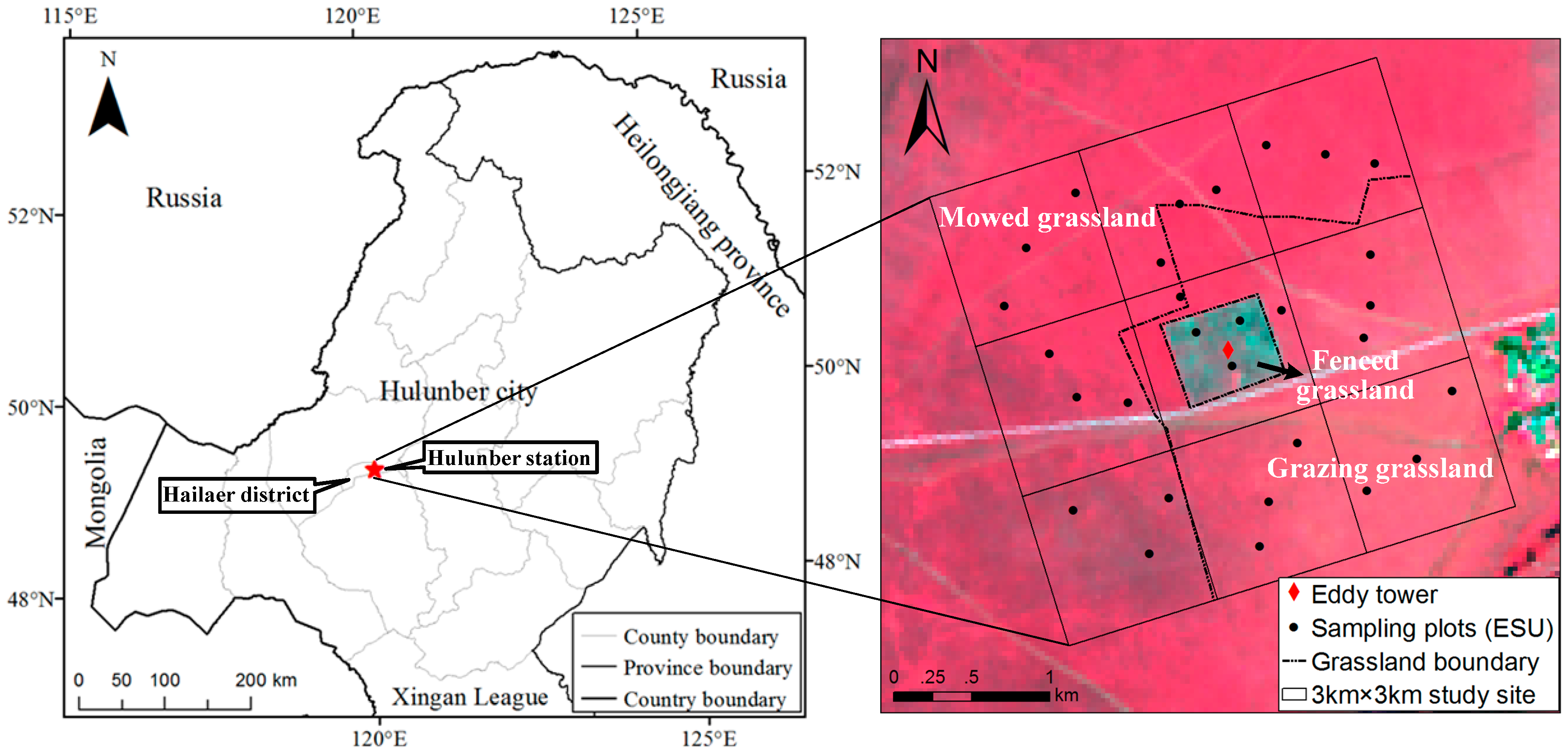
2.1. Study Site

Hulunber is the most complete and best-preserved natural meadow steppe on the Eurasian continent and has an amazing abundance of species endowed with high economic and ecological value. The Hulunber grassland ecosystem observation and research station (Hulunber station) is located in the middle of the Hulunber meadow steppe (49°20′24″ N, 119°59′44″ E), which is approximately 30 km northeast of the Hailaer District in Hulunber City, Inner Mongolia, China (Figure 1). The study area is located around the Hulunber station and covers an area of approximately 17 km × 7 km; the land cover is mainly meadow steppe, with 18.21 km² of cropland in the center (Figure 1). The region is characterized by a semi-arid inland climate with an annual mean precipitation of 350–400 mm and annual mean temperatures ranging from −3 to 1 °C. The average elevation is 626 m, and the terrain features a rolling surface that varies by as much as 200 m in elevation. Field observations were conducted on the grassland of the study area, primarily at the experimental site in an area of 3 km × 3 km that was centered at an eddy covariance flux tower. The site is homogeneous, and Leymus chinensis and Stipa baicalensis are the dominant grass species. The length of the growing season is approximately 140 days and lasts from May to September [33]. There are three grassland types at the site [34]: grazing grassland, which feeds cattle; mowed grassland that is used for silage; and fenced grassland, which is enclosed by a fence and has grown naturally for the past seven years without any external influence.

2.2. Sampling Design and Field Measurements

Field campaigns were performed during the growing seasons of 2014 and 2015. The experimental dates were 6 June, 1 July and 28 July in 2014 and 19 June, 10 August and 26 August in 2015. For regular experiments performed at the site, a two-scale sampling strategy designed by the VALERI project [35,36] was adopted to collect ground LAI data. The two scales used for the VALERI method were the site scale (at least a 3 km × 3 km square representative of the entire experimental site) and the elementary sampling unit scale (ESU, 30 m × 30 m, in this study corresponding to the pixel size of the remote sensing imagery). For the site scale, the 3 km × 3 km region was divided into nine 1 km × 1 km grids, and three to five ESUs were randomly selected in each grid. In total, 29 ESUs were chosen across the entire site. For each field campaign, the sampling plots were selected randomly from the 29 ESUs. A more detailed sampling protocol of this site has been described previously [37]. In addition, each ESU was located with a Global Positioning System (GPS) that was accurate to 2 m, ensuring that the measurements for each campaign were collected in the same location.

The effective LAI was measured using an LAI-2200C plant canopy analyzer (Li-Cor, Lincoln, NE, USA) with a 270° view cap. The LAI-2200C is an indirect, non-contact instrument that measures the gap fraction by observing diffuse radiation transmission through the canopy based on the assumption of a random leaf distribution within the canopy [38,39,40]. At each ESU, the effective LAI was measured at five points organized in a “cross” pattern in which each sample point was 15 m from the next point. One above-canopy and six below-canopy LAI-2200 measurements were obtained at each point to obtain one local LAI value, and five local LAI values were averaged to calculate a mean value for each ESU. The measurements were collected near sunrise or sunset to ensure nearly uniform sky illumination. From six field campaigns at the experimental site, a total of 690 LAI measurements were collected from 138 ESU plots.

2.3. Satellite Data

Chinese HJ-1A/1B (Huanjing (HJ)) charge coupled device (CCD) images were used as the remote sensing data source in this study. The HJ-1A/1B satellites are small civilian Earth-observing satellites that were launched on 6 September 2008 by China [41]. Among the payloads aboard the two satellites, multispectral CCD cameras are widely used in eco-environmental monitoring. Each satellite carries two CCD cameras, named CCD1 and CCD2, with a 700 km swath width, 48 h return period and 30 m pixel size. The HJ-1A/1B CCDs have three visible bands (blue (430–520 nm), green (520–600 nm) and red (630–690 nm)) and one near-infrared (NIR) band (760–900 nm) [42].

Six HJ-1A/1B CCD images corresponding to the dates of the field experiments were used in this study (

Table 1. Collection of remotely sensed images.

Experiment Date	6 June 2014	1 July 2014	28 July 2014	19 June 2015	10 August 2015	26 August 2015
Sensor for HJ Images	HJ1B CCD1	HJ1B CCD2	HJ1A CCD1	HJ1B CCD1	HJ1B CCD1	HJ1B CCD2
HJ Image Acquisition Date	6 June 2014	29 June 2014	29 July 2014	15 June 2015	10 August 2015	26 August 2015

). All images were radiometrically and geometrically corrected and were projected as UTM coordinates (WGS84 datum, Zone 50N). All images were high quality, and minimal (<10%) or no cloud contamination occurred at the site. To obtain the reflectance of the top of the canopy, the images were atmospherically corrected using the FLAASH program embedded in ENVI 4.8 software [43]. Two important parameters were used in the FLAASH program for atmospheric correction: aerosol optical depth and the water vapor column. These parameters were obtained using a Microtops II Sunphotometer (Solar Light Company, Inc., Glenside, PA, USA) during each field experiment. Finally, geometric correction was performed on all HJ-1A/1B CCD images using ground points collected in the field around the site; the correction accuracy was limited to within 1 pixel.

This study incorporated reflectance in four individual bands (blue, green, red, and NIR) and four VIs calculated from individual bands as independent variables. The vegetation indices included the simple ratio (SR), normalized difference vegetation index (NDVI), Atmospherically Resistant Vegetation Index (ARVI), and Wide Dynamic Range Vegetation Index (WDRVI), which exhibited strong and significant relationships with canopy LAI in the previous study [8,17,44]. These indices were computed using the following equations [45,46,47,48]:

$$NDVI=\frac{NIR-red}{NIR+red}$$

(1)

$$SR=\frac{NIR}{red}$$

(2)

$$ARVI=\frac{NIR-(red-\mathsf{\gamma }(blue-red))}{NIR+(red-\mathsf{\gamma }(blue-red))}$$

(3)

$$WDRVI=\frac{\mathsf{\alpha }\times NIR-red}{\mathsf{\alpha }\times NIR+red}$$

(4)

where $blue$, $red$, and $NIR$ refer to the band reflectance, $\mathsf{\gamma }$ is the atmospheric self-correcting factor (a value of 1 was recommended by Kaufman and Tanre [47] and is used in this study), and $\mathsf{\alpha }$ is the weighting coefficient (an $\mathsf{\alpha }$ value of 0.1 is used in this study [48]).

3. Methods

3.1. Partial Least Squares Regression (PLSR)

PLSR is a technique that reduces a large number of measured collinear spectral variables to a few non-correlated latent variables or factors, which must both summarize the variance of the explanatory variables well and correlate highly with the response variables [49,50]. The aim of PLSR is to build a linear model as follows:

$$Y=X\mathsf{\beta }+\mathsf{\epsilon }$$

(5)

where $Y$ is the mean-centered vector of the response variable, $X$ is the mean-centered matrix of the predictive variables, $\mathsf{\beta }$ is the matrix of coefficients, and $\mathsf{\epsilon }$ is the matrix of residuals. PLSR is closely related to principal component regression (PCR). In addition to PCR, PLSR uses both the predictor variables and response variable during the decomposition process and performs the decomposition on both the predictor variables and the response variable simultaneously, whereas PCR performs the decomposition on the predictor variables alone. The optimal number of factors for a PLS analysis is usually determined by minimizing the prediction residual error sum of squares (PRESS) statistic. The PRESS statistic was calculated through a cross-validation (CV) prediction for each model. The root mean squared error of cross validation (RMSCV) is also used to assess the predictive abilities of the PLS models [51]. The analysis was accomplished using the “pls” package [52] within the statistical software package R 3.2.0.

3.2. Artificial Neural Networks (ANNs)

ANNs are non-linear statistical learning approaches that have great potential for predictive modeling [53,54]. ANNs are composed of a large number of highly interconnected artificial neurons with weighted links that connect the input and output data through a learning process [14]. Various types of neural networks have been developed, and a layered feed-forward ANN with three layers is the most common ANN structure. In an ANN, information flows in a unidirectional forward mode from an input layer to an output layer via hidden layer(s). Neural networks attempt to identify the best solution based on network complexity through adaptive learning processes and the incorporation of various ancillary information (e.g., topography, sun angle, and ground data) [14]. A feed-forward neural network with a single hidden layer was used in this study. The analysis was accomplished using the “nnet” package within the statistical software package R 3.2.0 [55].

3.3. Random Forests (RFs)

An RF is an ensemble learning method that can be used for either classification or regression [56,57]. The algorithm is conceptually similar to the bagging decision tree but has extensions. An RF is a combination of tree predictors (n_tree) such that each tree depends on a collection of random variables sampled independently and then aggregates to produce accurate predictions. This method also shows better resistance to the over-fitting problem and to noise in the data compared with other regression methods [56]. Unlike bagging trees, an RF grows its trees from a randomly chosen subset of the total number of predictors at each splitting node (m_try), and the tree is allowed to grow fully without pruning. Each tree in the RF is independently grown to its maximum size based on a bootstrap sample from the training dataset (approximately two-thirds), and the remaining one-third of the samples are randomly left out. The left out samples are called the out-of-bag (OOB) samples, which are used to calculate an unbiased OOB error rate and the variable’s importance (measured by calculating the percent increase in the mean square error when the OOB data for each variable are permuted) [56,58]. At each binary split, the predictor that produces the best split is chosen from a random subset (m_try) of the entire predictor set (p); m_try is recognized as the main tuning parameter of an RF and must therefore be optimized [59,60]. The analysis was accomplished using the “randomForest” package [57] within the statistical software package R 3.2.0.

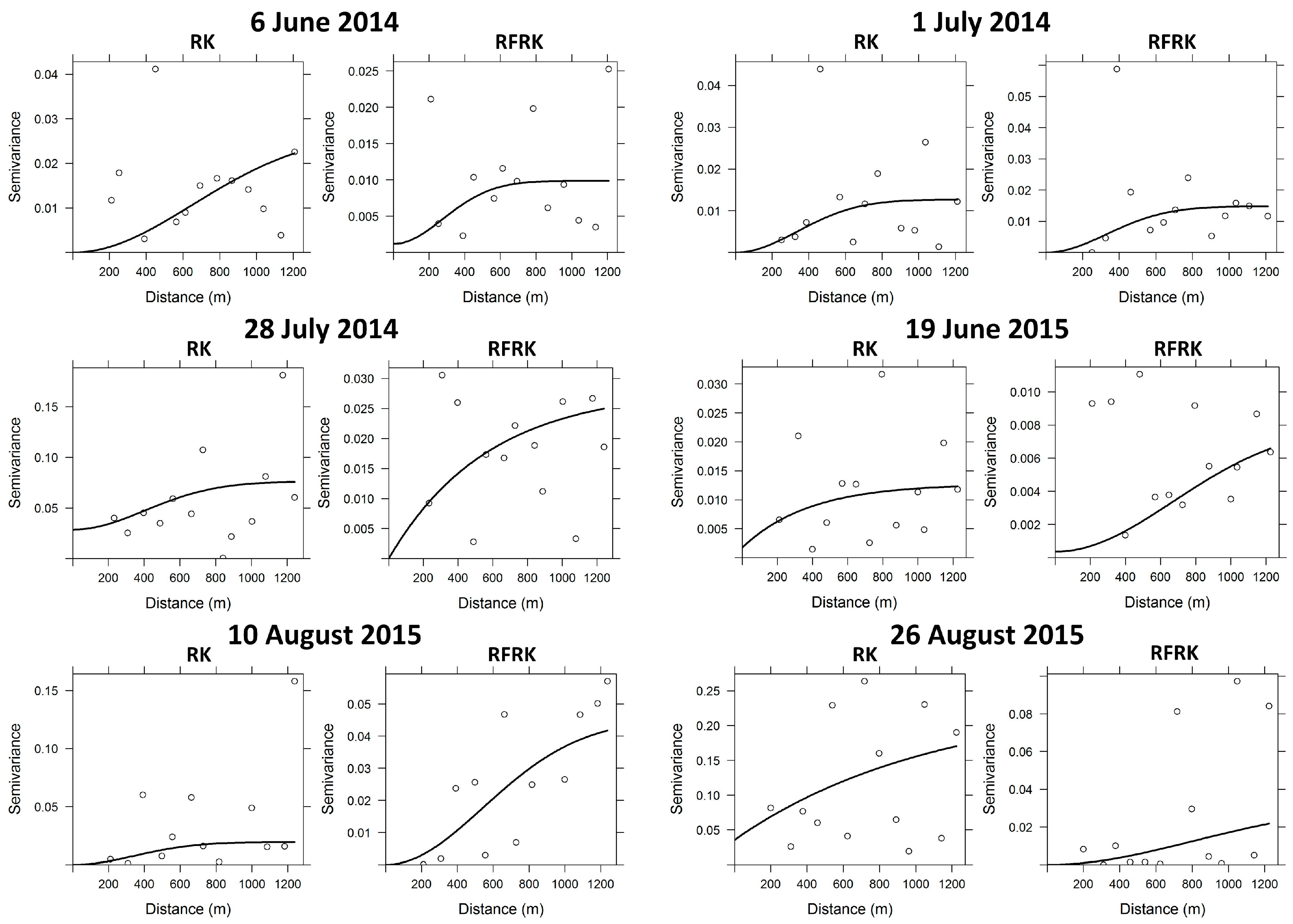
3.4. Regression Kriging (RK)

RK is a hybrid geostatistics method that combines a regression between the target variable and environmental variables with the ordinary kriging (OK) of the regression residuals. In RK, a liner regression is first used to fit the explanatory variation, and then kriging is used to fit the unexplained variation and to model the spatial variability of the data [61,62]. Finally, predictions at unvisited locations ${\widehat{z}}_{RK}(s_0)$ are performed by summing the predicted trend and residuals. The trend is commonly fitted using generalized least-squares regression, and the residuals are interpolated using OK [32,61].

$$z_{RK}(s_0)={\displaystyle \sum _{k=0}^p{\widehat{\mathsf{\beta }}}_k\times q_k(s_0)}+{\displaystyle \sum _{i=1}^n{\mathsf{\lambda }}_i\times e(s_i)}$$

(6)

where ${\widehat{\mathsf{\beta }}}_k$ corresponds to the estimated trend model coefficients, $q_k(s_0)$ represents the predictive variables at the location $s_0$, $e(s_i)$ is the regression residual, ${\mathsf{\lambda }}_i$ is the kriging weight determined by the spatial autocorrelation structure of the residual, and p is the number of auxiliary predictors. The analysis was accomplished using the “gstat” package [63] within the statistical software package R 3.2.0.

3.5. Random Forests Residuals Kriging (RFRK)

Although RF is a robust method that can improve prediction accuracy, this method ignores spatial autocorrelation information. To overcome this disadvantage, a hybrid method that combines RF and OK was developed and has been verified to generate much lower prediction errors and to yield a more realistic spatial distribution than the RF model [29]. RFRK is an extension of RF and is very similar to RK. RFRK also consists of trends and residuals. Here, the trend is modeled using RF; the residuals from RF are interpolated to prediction grids using OK, and the interpolated residuals are added to the RF prediction results to obtain the RFRK prediction results. The RFRK formula is as follows:

$$LA{I}_{RFRK}(s_i)=LA{I}_{RF}(s_i)+LA{I}_{OK}(s_i)$$

(7)

where $LA{I}_{RFRK}(s_i)$ is the predicted LAI at location $s_i$, $LA{I}_{RF}(s_i)$ is the trend modeled by RF, and $LA{I}_{OK}(s_i)$ is the residual interpolated by OK. This analysis was accomplished using the “randomForest” and “gstat” packages within the statistical software package R 3.2.0.

3.6. Model Implementation and Validation

In this study, we assumed that the ground measurements for each field campaign were conducted independently, and the temporal mixed effects of clustered data that originated from repeated measurements were not considered. To compare performance among models, the models were first implemented using predictive variables for the four spectral bands, and their performance for different grassland types and growing seasons was analyzed. The VIs were then gradually added to the input variables and were divided into five groups: four bands plus the best-performing VI, four bands plus one VI, four bands plus two VIs, four bands plus three VIs, and four bands plus four VIs. For each group, the LAI at the study site was first predicted using four bands plus the group number of VIs that were randomly combined. Then, after predicting LAI using all the combinations, each LAI prediction was assessed separately using ground measurements, and the accuracy indicator (root mean squared error (RMSE) in this study) was averaged to assess the performance of the group.

An independent dataset with 34 ESU plots was randomly selected from the original 138 samples to validate model performance, while the remaining 104 samples were used to train the models. The RMSE, mean absolute error (MAE) and coefficient of determination (R²) between measured and predicted values were calculated to assess the accuracy of each model:

$$RMSE=\sqrt{\frac{1}{n}{\displaystyle \sum _{i=1}^n{(y_i-{\widehat{y}}_i)}^2}}$$

(8)

$$MAE=\frac{1}{n}{\displaystyle \sum _{i=1}^n\left|y_i-{\widehat{y}}_i\right|}$$

(9)

where ${\widehat{y}}_i$ is the predicted LAI value, $y_i$ is the measured LAI value and $n$ is the number of measured values in the validation data. RMSE and MAE values close to zero and an R² value close to one indicate a better predictive capability of a model.

4. Results

4.1. Field LAI Measurements

Detailed summary statistics of the LAI measurements are shown in

Table 2. Descriptive statistics of the measured LAI dataset ¹.

Date		6 June 2014	1 July 2014	28 July 2014	19 June 2015	10 August 2015	26 August 2015
No. of training data		16	18	17	18	19	16
No. of validation data		4	8	5	6	6	5
Mowed grassland	Mean	1.32	2.56	2.35	1.57	1.80	1.43
	Min	1.00	2.01	1.45	1.19	0.88	1.05
	Max	1.50	3.22	2.75	2.03	2.56	2.12
	Stdev	0.19	0.30	0.42	0.24	0.50	0.30
Grazing grassland	Mean	0.94	1.68	1.21	0.93	0.83	0.83
	Min	0.61	0.81	0.69	0.77	0.69	0.77
	Max	1.45	2.73	2.64	1.17	1.02	0.89
	Stdev	0.30	0.59	0.64	0.13	0.10	0.05
Fenced grassland	Mean	- 2	-	-	-	3.40	3.50
	Min	-	-	-	-	3.40	3.44
	Max	-	-	-	-	3.41	3.56
	Stdev	-	-	-	-	0.01	0.08

¹ LAI in units of m²/m²; ² ”-”means no data are available for that day.

. Generally, the mean effective LAI values for the site ranged from 0.5–3.6 m²/m². During the early stage of the growing season (6 June 2014 and 19 June 2015), the mean and variability of the grass LAI values were relatively low (mean LAI value of 0.9–1.6 m²/m² and a standard deviation of 0.1–0.3 m²/m²). The middle of the growing stage (July in 2014) exhibited relatively high LAI values as well as increased variability. At the end of the growing season (August in 2015), the LAI variability in the mowed grassland remained at a high level due to grass cutting activity, while the grazing grassland showed a low LAI variability, and the fenced grassland still had a very high LAI value (LAI > 3.0 m²/m²).

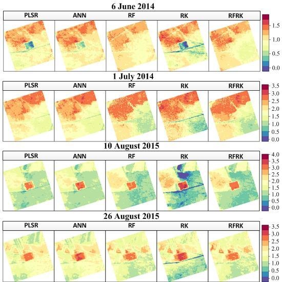
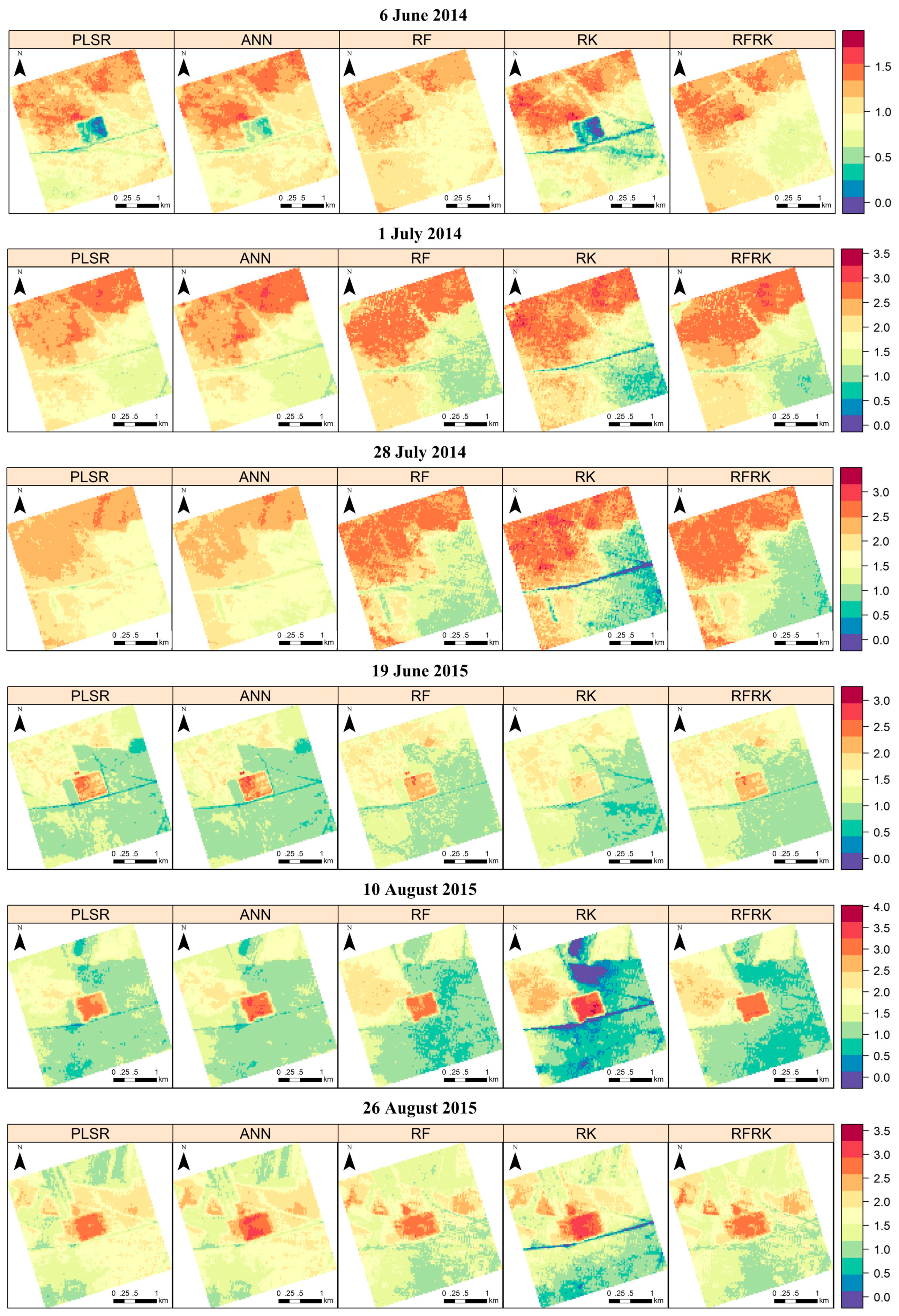
4.2. LAI Spatial Prediction Based on the Four Reflectance Bands

For the selection of tuning parameters used in the regression models, exploratory trials were conducted using the training dataset. For the PLSR, the first three principal components (PC) contained 99.01% of the predictor variable information and 74.17% of the response variable information (data not shown), which indicates that these three components could reasonably substitute the original inputs and explain the output information. For the ANN model, after trials, the optimized network with the best estimation performance was determined using 1 neuron in the hidden layers. For the RF model, n_tree was set to 500 (after exploratory trials using the training data). For m_try, the results from previous studies [59,64] showed that m_try optimization resulted in minimal improvements in RF predictions. We therefore used a predictive variable number of 2 in this analysis.

To apply the hybrid geostatistical methods (RK and RFRK), we utilized regression residual semivariograms and parameters obtained from the training dataset (Figure 2 and

Table 3. Parameters of the fitted empirical variogram models built from the residuals for RK and RFRK prediction.

Date	RK				RFRK
	Model	Nugget	Sill	Range	Model	Nugget	Sill	Range
6 June 2014	Gaussian	0.00	0.03	918.86	Gaussian	0.00	0.01	461.98
1 July 2014	Gaussian	0.00	0.02	560.13	Gaussian	0.00	0.02	609.90
28 July 2014	Gaussian	0.03	0.02	480.70	Exponential	0.00	0.03	595.52
19 June 2015	Exponential	0.00	0.03	2230.32	Gaussian	0.00	0.01	839.06
10 August 2015	Gaussian	0.00	0.02	441.76	Gaussian	0.00	0.05	769.84
26 August 2015	Exponential	0.04	0.20	1095.47	Gaussian	0.00	0.03	1105.05

), and the optimal variogram models were determined by the criteria of the sum of squared errors reported by the “gstat” package. An exponential or Gaussian model was fit to the sample semivariogram. For the RK, the models revealed the spatial autocorrelation of grassland LAI during the peak of the growing season with negligible nugget, a partial sill of 0.2, and a spatial range of 400–600 m. However, the models indicated a lower spatial dependence at the beginning and end of the growing season (larger partial sill and spatial range). For RFRK, the models also revealed aspects of spatial autocorrelation but performed worse than RK.

The LAI maps predicted from the five models are displayed in Figure 3. Overall, the prediction surfaces were similar in terms of the spatial patterns of grassland LAI. Differences between the mowed grassland, fenced grassland and grazing grassland were apparent from northwest to southeast. We observed a higher LAI value in the mowed grassland than in the grazing grassland throughout the growing season. The grazing grassland is used to feed cattle throughout the growing season, and the LAI value remained low. In the mowed grassland, the grass was fenced prior to August and then cut for silage. Thus, the LAI value was higher than the grazing grassland before it was cut and then sharply declined. The fenced grassland accumulated a considerable amount of litter prior to 2015, which delayed and then prevented the grass from growing, resulting in a lower LAI value in June 2014 but a similar value to the grazing grassland and mowed grassland on 1 July 2014 and 28 July 2014, respectively. At the beginning of 2015, the fenced grassland was burned and little litter remained. The grass grew quickly and displayed higher LAI values in 2015.

Table 4. Descriptive statistics of the LAI maps predicted by the study models.

6 June 2014					1 July 2014
	Min	Max	Mean	Stdev		Min	Max	Mean	Stdev
Measured LAI	0.61	1.50	1.10	0.31	Measured LAI	0.81	3.22	2.15	0.63
PLSR	0.00	1.64	1.02	0.25	PLSR	1.00	3.01	2.04	0.45
ANN	0.30	1.66	1.08	0.22	ANN	0.95	3.20	2.02	0.49
RF	0.78	1.48	1.07	0.16	RF	0.99	2.98	1.98	0.59
RK	0.00	1.77	0.96	0.33	RK	0.09	3.36	2.03	0.65
RFRK	0.60	1.58	1.05	0.21	RFRK	0.79	3.21	2.00	0.60
28 July 2014					19 June 2015
	Min	Max	Mean	Stdev		Min	Max	Mean	Stdev
Measured LAI	0.69	2.75	1.80	0.82	Measured LAI	0.77	2.03	1.27	0.38
PLSR	0.97	2.64	1.96	0.30	PLSR	0.00	2.86	1.19	0.37
ANN	0.82	2.64	1.86	0.33	ANN	0.20	3.05	1.16	0.38
RF	0.87	2.63	1.83	0.61	RF	0.65	2.80	1.29	0.35
RK	0.00	3.26	1.80	0.78	RK	0.10	2.11	1.23	0.35
RFRK	0.68	2.74	1.83	0.68	RFRK	0.60	2.79	1.28	0.36
10 August 2015					26 August 2015
	Min	Max	Mean	Stdev		Min	Max	Mean	Stdev
Measured LAI	0.69	3.41	1.51	0.82	Measured LAI	0.77	3.56	1.49	0.75
PLSR	0.10	3.11	1.38	0.43	PLSR	0.00	3.04	1.64	0.38
ANN	0.40	3.35	1.43	0.46	ANN	0.00	3.24	1.68	0.40
RF	0.80	3.01	1.41	0.57	RF	0.00	3.00	1.57	0.43
RK	0.00	3.76	1.25	0.79	RK	0.00	3.40	1.47	0.57
RFRK	0.65	3.26	1.39	0.62	RFRK	0.00	2.98	1.58	0.44

presents the general statistics for the predicted LAI maps. Compared to the measured LAI (Table 2), the predicted mean values approximated the measured values, whereas the minimum, maximum and standard deviation values were more varied. The RK predictions had higher standard deviation values (smaller minima and greater maxima) except for 19 June 2015 (Table 4). The LAI maps predicted by the PLSR model had a lower standard deviation value at the middle and end of the growing season (July and August), and the RF predictions exhibited greater minima.

4.3. Model Evaluation

Table 5. Validation of the predicted LAI maps using the measured validation dataset.

	MAE	RMSE	R2
PLSR	0.27	0.35	0.77
ANN	0.26	0.33	0.81
RF	0.21	0.27	0.89
RK	0.16	0.21	0.92
RFRK	0.17	0.23	0.91

presents a model evaluation result derived from an independent validation of the LAI maps using the validation dataset. RK was the most accurate method and exhibited the lowest RMSE (0.21 m²/m²) and MAE (0.16 m²/m²) values, as well as the highest R² (0.92) value. The accuracy of the RFRK predictions was nearly as good, with RMSE, MAE, and R² values of 0.23 m²/m², 0.17 m²/m², and 0.91, respectively, indicating an obvious improvement compared to the RF predictions. The predictive ability of the regression models was further improved by a geostatistical analysis of the regression residuals to compensate for the spatial autocorrelation information. However, the RF model still performed the best compared with all of the regression models due to its randomness and majority rule [56]. Although PLSR performed satisfactorily (RMSE of 0.35 m²/m², MAE of 0.27 m²/m², and R² of 0.77), this model was the worst of the five evaluated models (followed by the ANN model).

5. Discussion

5.1. LAI Predictions Based on the Four Reflectance Bands and VIs

The selected four VIs all had a good relationship with LAI; after conducting a correlation analysis between satellite-derived VIs and measured LAI, the R² values were higher than 0.65 (0.77, 0.74, 0.69, and 0.66 for SR, WDRVI, ARVI and NDVI, respectively), and the correlation coefficients were higher than 0.79 (0.88, 0.86, 0.83, and 0.79 for SR, WDRVI, ARVI and NDVI, respectively). To examine whether adding predictor variables would improve the model performance, the four VIs of SR, NDVI, ARVI and WDRVI were calculated, added to the original predictors, and divided into five groups (

Table 6. Validation of LAI predictions based on the four reflectance bands including VIs using the measured validation dataset.

	PLSR		ANN		RF		RK		RFRK
	MAE	RMSE	MAE	RMSE	MAE	RMSE	MAE	RMSE	MAE	RMSE
Four bands	0.274	0.353	0.264	0.328	0.209	0.269	0.164	0.212	0.173	0.231
Four bands + SR	0.216	0.279	0.221	0.277	0.197	0.252	0.180	0.261	0.150	0.217
Four bands + one VI	0.233	0.308	0.225	0.287	0.197	0.257	0.182	0.251	0.174	0.255
Four bands + two VIs	0.220	0.283	0.222	0.281	0.194	0.260	0.188	0.285	0.170	0.227
Four bands + three VIs	0.217	0.280	0.221	0.278	0.199	0.267	0.195	0.300	0.181	0.241
Four bands + four VIs	0.217	0.280	0.221	0.277	0.201	0.274	0.205	0.315	0.180	0.252

): four bands plus the best-performing VI (SR), four bands plus one VI, four bands plus two VIs, four bands plus three VIs, and four bands plus four VIs, detailed information was introduced in Section 3.6. The statistical analysis was performed separately for each of the five groups and the validation results are shown in Table 6. Generally, the performance of all the models, except for RK, with input variables of the four bands plus SR had the smallest prediction error with a small MAE and RMSE. For the PLSR and ANN models, adding VIs to the input variables improved the model performance; more predictors mean more information that can be used, resulting in better accuracy of the model. For the RF and RFRK models, adding more VIs did not result in more accurate predictions. By combining an ensemble of decision trees and randomly changing the predictors and training data for each decision tree, the RF model improved the prediction accuracy and demonstrated a more robust capacity with respect to the over-fitting problem and resisting noise data [56,57,59]. Furthermore, the RF model exhibited insensitivity to highly correlated predictors and irrelevant information [65,66]. Thus, VIs that were highly correlated with reflectance bands did not provide a considerable amount of additional knowledge to the RF model. For the RK model, the regression trend was implemented using multiple linear regression, and the multi-collinearity between independent variables stemming from the addition of VIs highly correlated with the reflectance band prevented the available information from being fully used, which generates ill-posed inversion problems [14,67]. The introduction of VIs to the RK model therefore resulted in poorer performance.

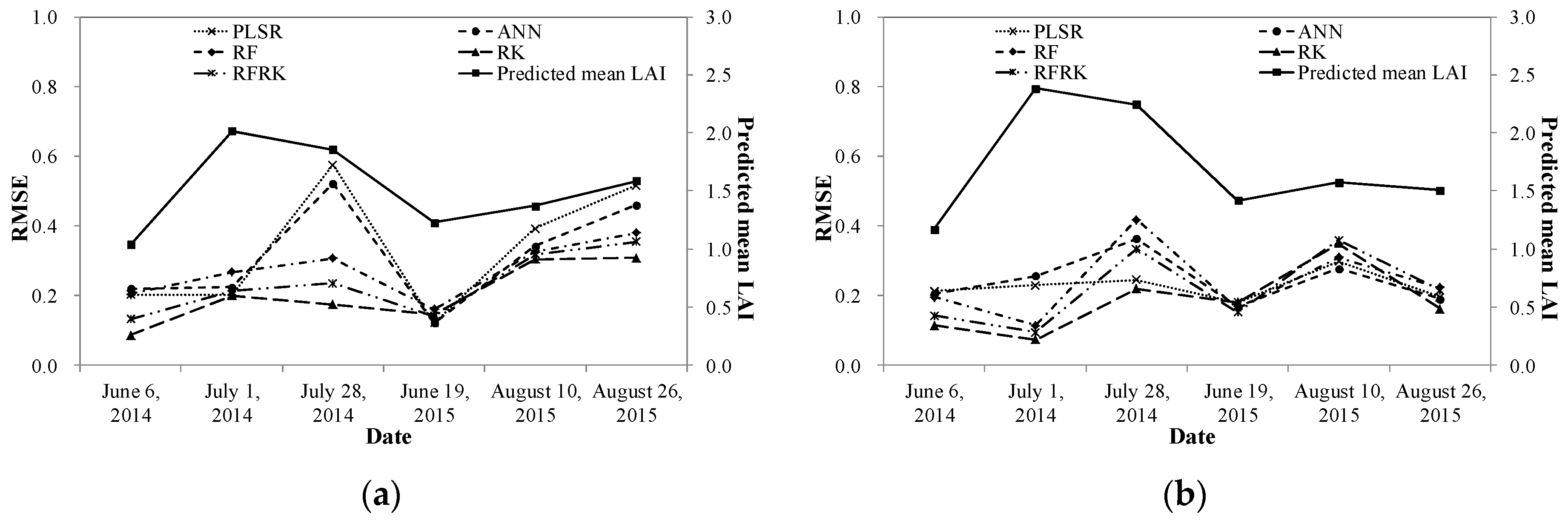
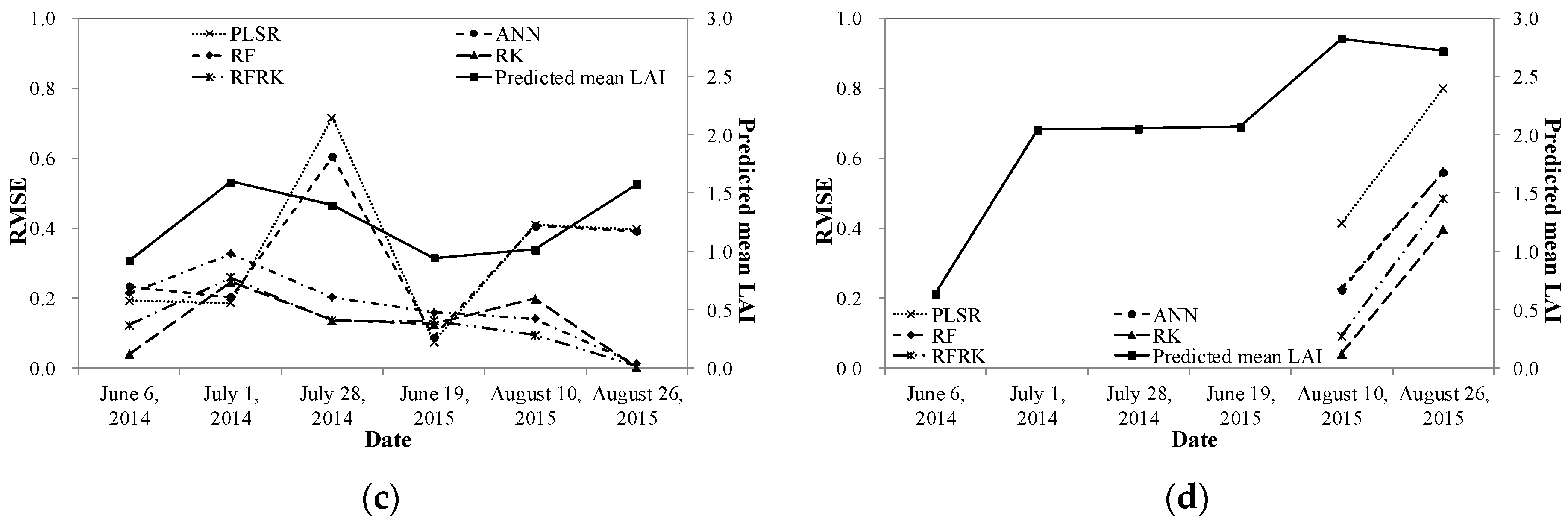
5.2. Model Performance in Different Grassland Types and at Different Growing Stages

Model performance was also assessed for different grassland types and different growing stages using the validation dataset. The RMSE between the predicted and measured LAIs is displayed in Figure 4. Across the entire site, the five models performed similarly and generated similar RMSEs (except for the prediction on 28 July 2014 for which PLSR and ANN generated a higher RMSE than the other three models, mainly due to the higher RMSE value of the grazing grassland). In addition, higher RMSE values were observed at the end of the growing season (August) for all five models. In the mowed grassland, the predicted LAI values were greater than 1 m²/m² on all six experimental dates. The five models exhibited a similar performance throughout the season but greater uncertainty was observed in the late-middle and end stages of the growing season (28 July 2014 and 10 August 2015), possibly resulting from an increasing amount of litter in the grassland [68,69]. After this time, grass cutting activity reduced the proportion of canopy litter, and the prediction uncertainty decreased on 26 August 2015. For the grazing grassland, the five models displayed more varied performance, especially the PLSR and ANN models. In contrast, the RF, RK and RFRK models performed steadily and exhibited low prediction error throughout the growing season. The PLSR and ANN models performed well with a smaller RMSE value during the beginning and early-middle stages of the growing season (June and early July). More uncertainty was observed during the late-middle and end stages of the growing season, possibly resulting from the continuous decline in vegetation cover due to grazing [70]. In the fenced grassland, the validation data existed for only two dates (10 August and 26 August in 2015). PLSR performed the worst. All five models generated considerable uncertainty for 26 August 2015 due to dead grasses.

Overall, the RF, RK and RFRK models performed well with a comparatively smaller and steady RMSE value throughout the growing season, while the performance of the PLSR and ANN models was more varied. Vegetation cover and grass litter were two factors that affected model performance.

5.3. Model Comparison and Study Limitations

In our study, the geostatistical methods proved to be the most accurate models in predicting grassland LAI, as indicated by the higher R² and lower RMSE values. Through geostatistical analysis of the residuals of the regression models, the prediction ability was further improved by supplying spatial autocorrelation information, showing better performance than the regression methods [21,23,71]. Despite these attractive properties, geostatistical methods are more sophisticated than simple mechanistic or kriging techniques. The requirements for the regression modeling are high, and the ground data accuracy will directly affect the fitted variogram parameters [32,61]. Moreover, issues associated with the transferability of results between images can also represent a serious limitation [23]. However, outside of the regression training area, the geostatistical analysis lost its power and generated more uncertainty.

The machine learning methods, such as ANNs and RFs, tend to be more powerful in predicting grassland LAI than the linear regression methods (e.g., PLSR) [17,19]. Through adaptive learning processes and the incorporation of more ancillary information, the best solution could be found without the constraints of linearity and multi-collinearity. Moreover, the ANN and RF models can also be used as variable selection tools to identify informative variables based on the network’s performance [14] or variable importance score [30,66]. However, the “black box” property of these approaches affected the model transparency [53], which prevents users from interpreting the results in physical terms [18]. In comparison, the recently popular RF method demonstrates a higher efficiency spatially and temporally compared with other machine learning methods due to its randomness and majority rule [59,72], and the model is recommended to be considered superior when combined with the hybrid inversion strategy [17,18]. The ANN method is susceptible to variation in the training data [19,73] and environmental interference information such as atmospheric scattering and background reflectance [17], which was also shown in this study and which reduced its spatial and temporal accuracy.

The PLSR also demonstrated certain power for predicting grassland LAI. The method was simple, computationally inexpensive and devoid of the co-linearity problem. However, the model was also very sensitive to some disturbing factors, such as surface property differences and satellite sun and viewing geometry. Therefore, this type of model cannot be applied to different site and sensor conditions [12,13]. The problem can be alleviated by using certain VIs that are sensitive to the target variables and relatively insensitive to interference factors [8,17,44].

The major source of uncertainty in this study is associated with the ground measurement data. For repeated measurements, the machine learning methods accounted for the spatial structure of errors, but the temporal structure error was neglected by assuming independent ground measurements between field campaigns. In contrast, certain methods that can handle mixed effects can be considered in future analyses [74,75]. Furthermore, HJ-CCD images and derived VIs were used in this study, and even though satisfactory results were obtained, the comparatively narrow spectral range still limited the more powerful VIs (e.g., reduced simple ratio (RSR) and cellulose absorption index (CAI)) used. In future studies, more powerful predictive variables derived from optical remote sensing datasets with broader spectral range (e.g., Landsat, Sentinel-2), light detection and ranging (LIDAR) [76] and synthetic aperture radar (SAR) [24] can be used, providing more information to train the dataset, which may lead to more accurate results. The study models were tested to determine their sensitivity to additional input variables (VIs); however, the impact of irrelevant information on model prediction was not tested in this study, and certain irrelevant and interference predictors can be introduced into the input variables to test their effect in future modeling. Finally, although the area of the study site is limited (only 3 km × 3 km), the biomes studied represent meadow steppes in northern China, and they can serve as a reference for future studies. Future research must also be expanded to larger area and new grassland types (desert grassland and typical grassland) that have not yet been adequately represented.

6. Conclusions

This study compared regression and hybrid geostatistical methods for predicting grassland LAI from Chinese HJ-1A/1B CCD images of northern China. The methods used were partial least squares regression, artificial neural networks, random forests, regression kriging, and random forests residuals kriging. Ground measurements of LAI were used for model training and validation. The two hybrid geostatistical models (RK and RFRK) resulted in more accurate predictions than the other models, and the regression residuals used to supply spatial autocorrelation information improved the prediction ability. The RF model was the most accurate of the regression models, while the other three models resulted in improved temporal performance throughout the growing season. The PLSR and ANN models were less accurate, and the PLSR model performed the worst. The temporal performances of PLSR, ANN, and PLSR were more varied, and their prediction accuracies were more susceptible to ground conditions, including vegetation cover and grass litter. By adding VIs to the predictor variables, the predictions of the PLSR and ANN models were markedly improved. However, the RF and RFRK models did not generate more accurate predictions, and the RK model generated poorer predictions due to inversion problems caused by the multi-collinearity between the independent input variables. These results should be further validated for a larger area, and more powerful predictive variables and remote sensing datasets (e.g., Landsat and Sentinel-2) should be utilized to develop accurate hybrid methods. Differential performance was observed for the methods evaluated herein for the meadow steppe of northern China, indicating that further comparisons for other applications, contexts, data quality and objectives are necessary.

References

1. Chen, J.M.; Black, T.A. Defining leaf area index for non-flat leaves. Plant Cell Environ. 1992, 15, 421–429. [Google Scholar] [CrossRef]
2. Running, S.W.; Nemani, R.R.; Peterson, D.L.; Band, L.E.; Potts, D.F.; Pierce, L.L.; Spanner, M.A. Mapping regional forest evapotranspiration and photosynthesis by coupling satellite data with ecosystem simulation. Ecology 1989, 70, 1090–1101. [Google Scholar] [CrossRef]
3. Sellers, P.J.; Dickinson, R.E.; Randall, D.A.; Betts, A.K.; Hall, F.G.; Berry, J.A.; Collatz, G.J.; Denning, A.S.; Mooney, H.A.; Nobre, C.A.; et al. Modeling the exchanges of energy, water, and carbon between continents and the atmosphere. Science 1997, 275, 502–509. [Google Scholar] [CrossRef] [PubMed]
4. Tian, Y.; Woodcock, C.E.; Wang, Y.; Privette, J.L.; Shabanov, N.V.; Zhou, L.; Zhang, Y.; Buermann, W.; Dong, J.; Veikkanen, B.; et al. Multiscale analysis and validation of the MODIS LAI product: I. Uncertainty assessment. Remote Sens. Environ. 2002, 83, 414–430. [Google Scholar] [CrossRef]
5. Wang, Y.; Woodcock, C.E.; Buermann, W.; Stenberg, P.; Voipio, P.; Smolander, H.; Häme, T.; Tian, Y.; Hu, J.; Knyazikhin, Y.; et al. Evaluation of the MODIS LAI algorithm at a coniferous forest site in Finland. Remote Sens. Environ. 2004, 91, 114–127. [Google Scholar] [CrossRef]
6. Behera, S.K.; Behera, M.D.; Tuli, R. An indirect method of estimating leaf area index in a tropical deciduous forest of India. Ecol. Indic. 2015, 58, 356–364. [Google Scholar] [CrossRef]
7. Olsoy, P.J.; Mitchell, J.J.; Levia, D.F.; Clark, P.E.; Glenn, N.F. Estimation of big sagebrush leaf area index with terrestrial laser scanning. Ecol. Indic. 2016, 61, 815–821. [Google Scholar] [CrossRef]
8. Broge, N.H.; Leblanc, E. Comparing prediction power and stability of broadband and hyperspectral vegetation indices for estimation of green leaf area index and canopy chlorophyll density. Remote Sens. Environ. 2000, 76, 156–172. [Google Scholar] [CrossRef]
9. Heiskanen, J. Estimating aboveground tree biomass and leaf area index in a mountain birch forest using ASTER satellite data. Int. J. Remote Sens. 2006, 27, 1135–1158. [Google Scholar] [CrossRef]
10. Cho, M.A.; Skidmore, A.; Corsi, F.; van Wieren, S.E.; Sobhan, I. Estimation of green grass/herb biomass from airborne hyperspectral imagery using spectral indices and partial least squares regression. Int. J. Appl. Earth Obs. 2007, 9, 414–424. [Google Scholar] [CrossRef]
11. Weiss, M.; Baret, F. Evaluation of canopy biophysical variable retrieval performances from the accumulation of large swath satellite data. Remote Sens. Environ. 1999, 70, 293–306. [Google Scholar] [CrossRef]
12. Verrelst, J.; Schaepman, M.E.; Koetz, B.; Kneubühler, M. Angular sensitivity analysis of vegetation indices derived from CHRIS/PROBA data. Remote Sens. Environ. 2008, 112, 2341–2353. [Google Scholar] [CrossRef]
13. Verrelst, J.; Schaepman, M.E.; Malenovský, Z.; Clevers, J.G.P.W. Effects of woody elements on simulated canopy reflectance: Implications for forest chlorophyll content retrieval. Remote Sens. Environ. 2010, 114, 647–656. [Google Scholar] [CrossRef] [Green Version]
14. Kimes, D.S.; Nelson, R.F.; Manry, M.T.; Fung, A.K. Review article: Attributes of neural networks for extracting continuous vegetation variables from optical and radar measurements. Int. J. Remote Sens. 1998, 19, 2639–2663. [Google Scholar] [CrossRef]
15. Durbha, S.S.; King, R.L.; Younan, N.H. Support vector machines regression for retrieval of leaf area index from multiangle imaging spectroradiometer. Remote Sens. Environ. 2007, 107, 348–361. [Google Scholar] [CrossRef]
16. Vuolo, F.; Neugebauer, N.; Bolognesi, S.; Atzberger, C.; Urso, G. Estimation of leaf area index using DEIMOS-1 data: Application and transferability of a semi-empirical relationship between two agricultural areas. Remote Sens. 2013, 5, 1274–1291. [Google Scholar] [CrossRef]
17. Liang, L.; Di, L.; Zhang, L.; Deng, M.; Qin, Z.; Zhao, S.; Lin, H. Estimation of crop LAI using hyperspectral vegetation indices and a hybrid inversion method. Remote Sens. Environ. 2015, 165, 123–134. [Google Scholar] [CrossRef]
18. Verrelst, J.; Camps-Valls, G.; Muñoz-Marí, J.; Rivera, J.P.; Veroustraete, F.; Clevers, J.G.P.W.; Moreno, J. Optical remote sensing and the retrieval of terrestrial vegetation bio-geophysical properties—A review. ISPRS J. Photogramm. 2015, 108, 273–290. [Google Scholar] [CrossRef]
19. Verrelst, J.; Rivera, J.P.; Veroustraete, F.; Muñoz-Marí, J.; Clevers, J.G.P.W.; Camps-Valls, G.; Moreno, J. Experimental Sentinel-2 LAI estimation using parametric, non-parametric and physical retrieval methods—A comparison. ISPRS J. Photogramm. 2015, 108, 260–272. [Google Scholar] [CrossRef]
20. Williams, M.; Bell, R.; Spadavecchia, L.; Street, L.E.; Van Wijk, M.T. Upscaling leaf area index in an arctic landscape through multiscale observations. Glob. Chang. Biol. 2008, 14, 1517–1530. [Google Scholar] [CrossRef]
21. Berterretche, M.; Hudak, A.T.; Cohen, W.B.; Maiersperger, T.K.; Gower, S.T.; Dungan, J. Comparison of regression and geostatistical methods for mapping leaf area index (LAI) with Landsat ETM+ data over a boreal forest. Remote Sens. Environ. 2005, 96, 49–61. [Google Scholar] [CrossRef]
22. Martinez, B.; Cassiraga, E.; Camacho, F.; Garcia-Haro, J. Geostatistics for mapping leaf area index over a cropland landscape: Efficiency sampling assessment. Remote Sens. 2010, 2, 2584–2606. [Google Scholar] [CrossRef]
23. Castillo-Santiago, M.Á.; Ghilardi, A.; Oyama, K.; Hernández-Stefanoni, J.L.; Torres, I.; Flamenco-Sandoval, A.; Fernández, A.; Mas, J.-F. Estimating the spatial distribution of woody biomass suitable for charcoal making from remote sensing and geostatistics in central Mexico. Energy Sustain. Dev. 2013, 17, 177–188. [Google Scholar] [CrossRef]
24. Galeana-Pizaña, J.M.; López-Caloca, A.; López-Quiroz, P.; Silván-Cárdenas, J.L.; Couturier, S. Modeling the spatial distribution of above-ground carbon in mexican coniferous forests using remote sensing and a geostatistical approach. Int. J. Appl. Earth Obs. 2014, 30, 179–189. [Google Scholar] [CrossRef]
25. Heuvelink, G.B.M.; Griffith, D.A. Space-Time geostatistics for geography: A case study of radiation monitoring across parts of germany. Geogr. Anal. 2010, 42, 161–179. [Google Scholar] [CrossRef]
26. Ge, Y.; Liang, Y.; Wang, J.; Zhao, Q.; Liu, S. Upscaling sensible heat fluxes with area-to-area regression kriging. IEEE Geosci. Remote Sens. Lett. 2015, 12, 656–660. [Google Scholar]
27. Hernández-Stefanoni, J.L.; Alberto Gallardo-Cruz, J.; Meave, J.A.; Dupuy, J.M. Combining geostatistical models and remotely sensed data to improve tropical tree richness mapping. Ecol. Indic. 2011, 11, 1046–1056. [Google Scholar] [CrossRef]
28. Viana, H.; Aranha, J.; Lopes, D.; Cohen, W.B. Estimation of crown biomass of pinus pinaster stands and shrubland above-ground biomass using forest inventory data, remotely sensed imagery and spatial prediction models. Ecol. Model. 2012, 226, 22–35. [Google Scholar] [CrossRef]
29. Guo, P.; Li, M.; Luo, W.; Tang, Q.; Liu, Z.; Lin, Z. Digital mapping of soil organic matter for rubber plantation at regional scale: An application of random forest plus residuals kriging approach. Geoderma 2015, 237–238, 49–59. [Google Scholar] [CrossRef]
30. Were, K.; Bui, D.T.; Dick, Ø.B.; Singh, B.R. A comparative assessment of support vector regression, artificial neural networks, and random forests for predicting and mapping soil organic carbon stocks across an afromontane landscape. Ecol. Indic. 2015, 52, 394–403. [Google Scholar] [CrossRef]
31. Yang, F.; Sun, J.; Fang, H.; Yao, Z.; Zhang, J.; Zhu, Y.; Song, K.; Wang, Z.; Hu, M. Comparison of different methods for corn LAI estimation over northeastern China. Int. J. Appl. Earth Obs. 2012, 18, 462–471. [Google Scholar]
32. Hengl, T.; Heuvelink, G.B.M.; Rossiter, D.G. About regression-kriging: From equations to case studies. Comput. Geosci. 2007, 33, 1301–1315. [Google Scholar] [CrossRef]
33. Tang, H.; Li, Z.; Zhu, Z.; Chen, B.; Zhang, B.; Xin, X. Variability and climate change trend in vegetation phenology of recent decades in the greater Khingan mountain area, northeastern China. Remote Sens. 2015, 7, 11914–11932. [Google Scholar] [CrossRef]
34. Wu, Q.; Jin, Y.; Bao, Y.; Hai, Q.; Yan, R.; Chen, B.; Zhang, H.; Zhang, B.; Li, Z.; Li, X.; et al. Comparison of two inversion methods for leaf area index using HJ-1 satellite data in a temperate meadow steppe. Int. J. Remote Sens. 2015, 36, 1–16. [Google Scholar] [CrossRef]
35. De Kauwe, M.G.; Disney, M.I.; Quaife, T.; Lewis, P.; Williams, M. An assessment of the MODIS collection 5 leaf area index product for a region of mixed coniferous forest. Remote Sens. Environ. 2011, 115, 767–780. [Google Scholar] [CrossRef]
36. VAlidation of Land European Remote sensing Instruments. Available online: http://w3.avignon.inra.fr/valeri/ (accessed on 18 January 2016).
37. Li, Z.; Tang, H.; Xin, X.; Zhang, B.; Wang, D. Assessment of the MODIS LAI product using ground measurement data and HJ-1A/1A imagery in the meadow steppe of Hulunber, China. Remote Sens. 2014, 6, 6242–6265. [Google Scholar] [CrossRef]
38. Chen, J.M.; Pavlic, G.; Brown, L.; Cihlar, J.; Leblanc, S.G.; White, H.P.; Hall, R.J.; Peddle, D.R.; King, D.J.; Trofymow, J.A.; et al. Derivation and validation of Canada-wide coarse-resolution leaf area index maps using high-resolution satellite imagery and ground measurements. Remote Sens. Environ. 2002, 80, 165–184. [Google Scholar] [CrossRef]
39. Welles, J.M.; Norman, J.M. Instrument for indirect measurement of canopy architecture. Agron. J. 1991, 83, 818–825. [Google Scholar] [CrossRef]
40. Fang, H.; Li, W.; Wei, S.; Jiang, C. Seasonal variation of leaf area index (LAI) over paddy rice fields in NE China: Intercomparison of destructive sampling, LAI-2200, digital hemispherical photography (DHP), and ACCUPAR methods. Agric. For. Meteorol. 2014, 198–199, 126–141. [Google Scholar] [CrossRef]
41. China Centre for Resources Satellite Data and Application. Available online: http://www.cresda.com (accessed on 18 January 2016).
42. Bo, J.; Shunlin, L.; Townshend, J.R.; Dodson, Z.M. Assessment of the radiometric performance of Chinese HJ-1 satellite CCD instruments. IEEE J. Sel. Top. Appl. Earth Obs. Remote Sens. 2013, 6, 840–850. [Google Scholar]
43. Agrawal, G.; Sarup, J.; Bhopal, M. Comparision of QUAC and FLAASH atmospheric correction modules on EO-1 hyperion data of Sanchi. Int. J. Adv. Eng. Sci. Technol. 2011, 4, 178–186. [Google Scholar]
44. Baret, F.; Guyot, G. Potentials and limits of vegetation indices for LAI and APAR assessment. Remote Sens. Environ. 1991, 35, 161–173. [Google Scholar] [CrossRef]
45. Rouse, J.W., Jr.; Haas, R.; Schell, J.; Deering, D. Monitoring vegetation systems in the great plains with Erts. NASA Spec. Publ. 1974, 351, 309. [Google Scholar]
46. Jordan, C.F. Derivation of leaf-area index from quality of light on the forest floor. Ecology 1969, 50, 663–666. [Google Scholar] [CrossRef]
47. Kaufman, Y.J.; Tanre, D. Atmospherically resistant vegetation index (ARVI) for EOS-MODIS. IEEE Trans. Geosci. Remote Sens. 1992, 30, 261–270. [Google Scholar] [CrossRef]
48. Gitelson, A.A. Wide dynamic range vegetation index for remote quantification of biophysical characteristics of vegetation. J. Plant Physiol. 2004, 161, 165–173. [Google Scholar] [CrossRef] [PubMed]
49. Darvishzadeh, R.; Atzberger, C.; Skidmore, A.; Schlerf, M. Mapping grassland leaf area index with airborne hyperspectral imagery: A comparison study of statistical approaches and inversion of radiative transfer models. ISPRS J. Photogramm. 2011, 66, 894–906. [Google Scholar] [CrossRef]
50. Geladi, P.; Kowalski, B.R. Partial least-squares regression: A tutorial. Anal. Chim. Acta 1986, 185, 1–17. [Google Scholar] [CrossRef]
51. Pandit, C.M.; Filippelli, G.M.; Li, L. Estimation of heavy-metal contamination in soil using reflectance spectroscopy and partial least-squares regression. Int. J. Remote Sens. 2010, 31, 4111–4123. [Google Scholar] [CrossRef]
52. Mevik, B.-H.; Wehrens, R. The PLS package: Principal component and partial least squares regression in R. J. Stat. Softw. 2007, 18, 1–24. [Google Scholar] [CrossRef]
53. Lek, S.; Guégan, J.F. Artificial neural networks as a tool in ecological modelling, an introduction. Ecol. Model. 1999, 120, 65–73. [Google Scholar] [CrossRef]
54. Lek, S.; Giraudel, J.L.; Guégan, J.F. Neuronal networks: Algorithms and architectures for ecologists and evolutionary ecologists. In Artificial Neuronal Networks; Lek, S., Guégan, J.-F., Eds.; Springer Berlin Heidelberg: Berlin, Germany; Heidelberg, Germany, 2000; pp. 3–27. [Google Scholar]
55. Team, R.C. R: A Language and Environment for Statistical Computing. 2013. Available online: http://cran.fiocruz.br/web/packages/dplR/vignettes/timeseries-dplR.pdf (accessed on 4 April 2016).
56. Breiman, L. Random forests. Mach. Learn. 2001, 45, 5–32. [Google Scholar] [CrossRef]
57. Liaw, A.; Wiener, M. Classification and regression by randomforest. R News 2002, 2, 18–22. [Google Scholar]
58. Prasad, A.M.; Iverson, L.R.; Liaw, A. Newer classification and regression tree techniques: Bagging and random forests for ecological prediction. Ecosystems 2006, 9, 181–199. [Google Scholar] [CrossRef]
59. Heung, B.; Bulmer, C.E.; Schmidt, M.G. Predictive soil parent material mapping at a regional-scale: A random forest approach. Geoderma 2014, 214–215, 141–154. [Google Scholar] [CrossRef]
60. Svetnik, V.; Liaw, A.; Tong, C.; Culberson, J.C.; Sheridan, R.P.; Feuston, B.P. Random forest: A classification and regression tool for compound classification and QSAR modeling. J. Chem. Inf. Comput. Sci. 2003, 43, 1947–1958. [Google Scholar] [CrossRef] [PubMed]
61. Hengl, T.; Heuvelink, G.B.M.; Stein, A. A generic framework for spatial prediction of soil variables based on regression-kriging. Geoderma 2004, 120, 75–93. [Google Scholar] [CrossRef]
62. Odeh, I.O.A.; McBratney, A.B.; Chittleborough, D.J. Further results on prediction of soil properties from terrain attributes: Heterotopic cokriging and regression-kriging. Geoderma 1995, 67, 215–226. [Google Scholar] [CrossRef]
63. Pebesma, E.J. Multivariable geostatistics in S: The gstat package. Comput. Geosci. 2004, 30, 683–691. [Google Scholar] [CrossRef]
64. Hultquist, C.; Chen, G.; Zhao, K. A comparison of gaussian process regression, random forests and support vector regression for burn severity assessment in diseased forests. Remote Sens. Lett. 2014, 5, 723–732. [Google Scholar] [CrossRef]
65. Genuer, R.; Poggi, J.-M.; Tuleau-Malot, C. Variable selection using random forests. Pattern Recogn. Lett. 2010, 31, 2225–2236. [Google Scholar] [CrossRef]
66. Genuer, R.; Poggi, J.-M.; Tuleau, C. Random Forests: Some Methodological Insights. 2008. Available online: http://arxiv.org/pdf/0811.3619v1.pdf (accessed on 4 April 2016).
67. Huang, C.; Townshend, J.R.G. A stepwise regression tree for nonlinear approximation: Applications to estimating subpixel land cover. Int. J. Remote Sens. 2003, 24, 75–90. [Google Scholar] [CrossRef]
68. Deng, Y.; Liu, X.N.; Yan, R.R.; Wang, X.; Yang, G.X.; Ren, Z.C.; Xin, X.P. Soil respiration of Hulunber meadow steppe and response of its controlling factors to different grazing intensities. Acta Pratacult. Sin. 2013, 22, 22–29. (In Chinese) [Google Scholar]
69. Yan, R.; Tang, H.; Xin, X.; Chen, B.; Murray, P.J.; Yan, Y.; Wang, X.; Yang, G. Grazing intensity and driving factors affect soil nitrous oxide fluxes during the growing seasons in the Hulunber meadow steppe of China. Environ. Res. Lett. 2016, 11, 054004. [Google Scholar] [CrossRef]
70. Yan, R.; Xin, X.; Zhang, B.; Yan, Y.; Yang, G. Influence of cattle grazing gradient on plant community characteristics in Hulunber meadow steppe. Chin. J. Grassl. 2010, 32, 62–67. (In Chinese) [Google Scholar]
71. Propastin, P. Modifying geographically weighted regression for estimating aboveground biomass in tropical rainforests by multispectral remote sensing data. Int. J. Appl. Earth Obs. 2012, 18, 82–90. [Google Scholar] [CrossRef]
72. Ramoelo, A.; Cho, M.A.; Mathieu, R.; Madonsela, S.; van de Kerchove, R.; Kaszta, Z.; Wolff, E. Monitoring grass nutrients and biomass as indicators of rangeland quality and quantity using random forest modelling and Worldview-2 data. Int. J. Appl. Earth Obs. 2015, 43, 43–54. [Google Scholar] [CrossRef]
73. Papale, D.; Black, T.A.; Carvalhais, N.; Cescatti, A.; Chen, J.; Jung, M.; Kiely, G.; Lasslop, G.; Mahecha, M.D.; Margolis, H.; et al. Effect of spatial sampling from european flux towers for estimating carbon and water fluxes with artificial neural networks. J. Geophys. Res. Biogeosci. 2015, 120, 1941–1957. [Google Scholar] [CrossRef]
74. Isik, F.; Ozden, G. Estimating compaction parameters of fine- and coarse-grained soils by means of artificial neural networks. Environ. Earth Sci. 2013, 69, 2287–2297. [Google Scholar] [CrossRef]
75. Hajjem, A.; Bellavance, F.; Larocque, D. Mixed-effects random forest for clustered data. J. Stat. Comput. Sim. 2014, 84, 1313–1328. [Google Scholar] [CrossRef]
76. Pope, G.; Treitz, P. Leaf area index (LAI) estimation in boreal mixedwood forest of Ontario, Canada using light detection and ranging (LIDAR) and WorldView-2 imagery. Remote Sens. 2013, 5, 5040–5063. [Google Scholar] [CrossRef]
Figure 1. Site location and sampling plots (background: Landsat-8 OLI false-color composite image (5, 4, and 3) from 13 June 2013).
Remotesensing 08 00632 g001
Figure 2. Experimental variograms of regression residuals for grassland LAI.
Remotesensing 08 00632 g002
Figure 3. Spatially distributed maps of grassland LAI.
Remotesensing 08 00632 g003
Figure 4. RMSE of the validation results for different grassland types using the measured validation dataset for: (a) the whole site; (b) mowed grassland; (c) grazing grassland; and (d) fenced grassland. The predicted mean LAI is the mean value averaged from the maps predicted using the five models; the missing RMSE in the fenced grassland indicates that no validation data were available for that day.
Remotesensing 08 00632 g004aRemotesensing 08 00632 g004b