Investigation of Spectral Band Requirements for Improving Retrievals of Phytoplankton Functional Types

Abstract

Studying phytoplankton functional types (PFTs) from space is possible due to recent advances in remote sensing. Though a variety of products are available, the limited number of wavelengths available compared to the number of model parameters needed to be retrieved is still a major problem in using ocean-color data for PFT retrievals. Here, we investigated which band placement could improve retrievals of three particular PFTs (diatoms, coccolithophores and cyanobacteria). In addition to analyzing dominant spectral features in the absorption spectra of the target PFTs, two previously-developed methods using measured spectra were applied to simulated data. Such a synthetic dataset allowed for significantly increasing the number of scenarios and enabled a full control over parameters causing spectral changes. We evaluated the chosen band placement by applying an adapted ocean reflectance inversion, as utilized in the generalized inherent optical properties (GIOP) retrieval. Results show that the optimal band settings depend on the method applied to determine the bands placement, as well as on the internal variability of the dataset investigated. Therefore, continuous hyperspectral instruments would be most beneficial for discriminating multiple PFTs, though a small improvement in spectral sampling and resolution does not significantly modify the results. Bands, which could be added to future instruments (e.g., Ocean and Land Colour Instrument (OLCI) instrument on the upcoming Sentinel-3B,-3C,-3D, etc., and further satellites) in order to enhance PFT retrieval capabilities, were also determined.

1. Introduction

Different phytoplankton functional types (PFTs) play various roles in the carbon and other biogeochemical cycles and respond differently to changes in environmental conditions [1]. While PFTs and their specific roles in the ecosystems have been incorporated into ecological and biogeochemical modeling studies (e.g., [2]), recent advances in satellite ocean color observations have enabled retrieving global information on the composition of the phytoplankton community.

A number of different bio-optical and ecological algorithms have been developed to identify and differentiate between PFTs, size classes (PSCs) and taxonomic composition [1]. Though a variety of products are available, they significantly differ in the type of information they provide, their assumptions and their performance on different spatial and temporal scales. The limited number of wavelengths available, compared to the number of model parameters needed to be retrieved to resolve the complex spectral features within the satellite data, is a major problem in using ocean-color data for PFT retrievals [1]. Hence, improved spectral resolution and sampling of future satellite-borne instruments are expected to allow the retrieval of additional spectral properties characteristic for PFTs. With planned missions, much of the ocean color community has been asking what sensor spectral bands will be required to improve on the PFT retrievals proof of concept that have already been established, but have limitations with existing instruments. This manuscript directly addresses that desired knowledge from a modeled framework and is a contribution toward defining spectral requirements and ideal band placement.

A number of previous studies analyzed measured remote sensing reflectances ($R_{rs}\left(\lambda \right)$) or absorption spectra to determine the band placement for obtaining the best retrieval results. For example, Hoepffner and Sathyendranath [3] decomposed absorption spectra into Gaussian absorption bands, while Lee et al. [4] and Isada et al. [5] performed derivative analysis on $R_{rs}\left(\lambda \right)$ and phytoplankton absorption spectra, respectively. In addition to different methods, different datasets were analyzed in the above-mentioned studies, ranging from cultures, through a spatially and temporally small-scale set of in situ samples, to a larger set of measurements covering various marine environments. Similar, but different bands were obtained depending on the study, and no final consensus was met. Furthermore, these studies suggested which bands might have greater importance for retrieving PFTs, but did not attempt to test their actual performance while retrieving PFTs. The choice of the most appropriate band placement might also vary depending on the design of a PFT retrieval, and thus, more investigation is required, depending on the chosen algorithm.

On the other hand, it is the continuous hyperspectral data that might offer the best possibility to retrieve PFTs, since they provide the highest number of bands at a given interval, and various algorithms can be applied to them and further adjusted. This might be possible with some anticipated missions (e.g., the Environmental Mapping and Analysis Program (EnMAP) mission [6] or the Pre-Aerosol, Clouds, and ocean Ecosystem (PACE) mission [7]), which will have improved spectral resolution and spectral sampling. Xi et al. [8] recently studied if such hyperspectral data could possibly allow the discrimination of several PFTs from remote sensing reflectances. They examined the performance of the spectral fourth derivative analysis and a clustering technique applied to simulated remote sensing reflectances, using as input measured hyperspectral absorption spectra of laboratory phytoplankton cultures and phytoplankton absorption spectra inverted with the quasi-analytical algorithm (QAA), to differentiate six taxonomic groups. The differentiation performed most effective on measured phytoplankton absorption, then better on hyperspectral $R_{rs}\left(\lambda \right)$ than on QAA-inverted spectra (due to errors induced by the inversion algorithm, likely due to assumptions made in spectral shapes of optical components, etc., within QAA). However, culture-based data of single species were considered in this study, unlikely for natural conditions in which an algorithm needs to perform on satellite ocean color data.

Other efforts to retrieve PFTs have been based on applying ocean reflectance inversion models to measured and modeled reflectances [9,10]. Such inversion methods, which minimize the difference between observations and the model, are susceptible to the choice of parameters and may not yield satisfactory solutions if the model is not sufficiently representing reality and if components assigned to absorption and backscattering are too few or are poorly assigned [1]. Werdell et al. [9,10] applied ocean reflectance inversion models to MODIS data to identify N. miliaris in the Arabian Sea, but they were only able to infer the presence or absence of N. miliaris, suggesting caution when interpreting the absolute magnitude of the retrievals. They demonstrated, however, that new satellite missions with increased spectral resolution should improve the identification of phytoplankton community structure from space.

Satellite data of high spectral resolution have been already applied in the ocean color satellite remote sensing. Specifically, the data from the atmospheric mission SCIAMACHY (Scanning Imaging Absorption Spectrometer for Atmospheric Chartography) [11,12] have been used to retrieve PFTs [13,14], light availability [15] and chlorophyll a(chl-a) fluorescence [16]. However, these data of high spectral resolution (0.26–0.44 nm in the UV-visible range) had also a large pixel size (∼30 km by 60 km). Since atmospheric correction of SCIAMACHY data would have to handle strong atmospheric absorbers and heterogeneity of big pixels, Bracher et al. [13] designed the algorithm PhytoDOAS (an extension of the Differential Optical Absorption Spectroscopy for oceanic phytoplankton groups) to retrieve diatoms and cyanobacteria directly from top of atmosphere radiances, by separating their high frequency absorptions from each other and relevant atmospheric absorbers, while accounting for broad band effects by using a low order polynomial. Later, Sadeghi et al. [14] adjusted the algorithm to additionally retrieve coccolithophores with SCIAMACHY. While these studies explored the possibility of applying hyperspectral satellite data to ocean color observations despite the instrumental limitations, future dedicated ocean color missions are expected to have increased spectral resolution and coverage together with improved spatial coverage, as compared to current multispectral missions. They also will be atmospherically corrected and, hence, directly supply remote sensing reflectances to be used in ocean color retrievals.

Here, we tested which band placement would be the most optimal to retrieve three above-mentioned PFTs from multispectral instruments: diatoms, coccolithophores and cyanobacteria. In the present study, we focused on these PFTs, since they constitute the only ones being retrieved globally and simultaneously from their optical signatures. Their previous retrievals with SCIAMACHY data showed that their spectral characteristics differ enough to allow their discrimination from satellite data. In addition to analyzing dominating spectral features in the absorption spectra of specific PFTs, two methods, which were previously applied to measured spectra [4,5], were applied to simulated data. This synthetic dataset allows for significantly increasing the number of scenarios and enables a full control over parameters that lead to the variability within the dataset. In addition, basic modeling approaches simplify the dataset and represent the best possibility where all of the variability is correctly assigned to the three considered PFTs. We determined the optimal band placements with the different approaches. Afterwards, we tested the feasibility of retrieving diatoms, coccolithophores and cyanobacteria with the generalized IOP (GIOP) software applied to the simulated data and the selected band placements. For a more comprehensive comparison, GIOP retrievals were also run on continuous hyperspectral data with various spectral sampling and resolution. Different resolutions and band placements were examined in terms of the best performance of these spectral inversion retrievals.

2. Materials and Methods

Three different methods (described below) were applied to examine the placement of spectral bands to retrieve different PFTs. The flowchart of the consecutive steps involved in this process is shown in Figure 1.

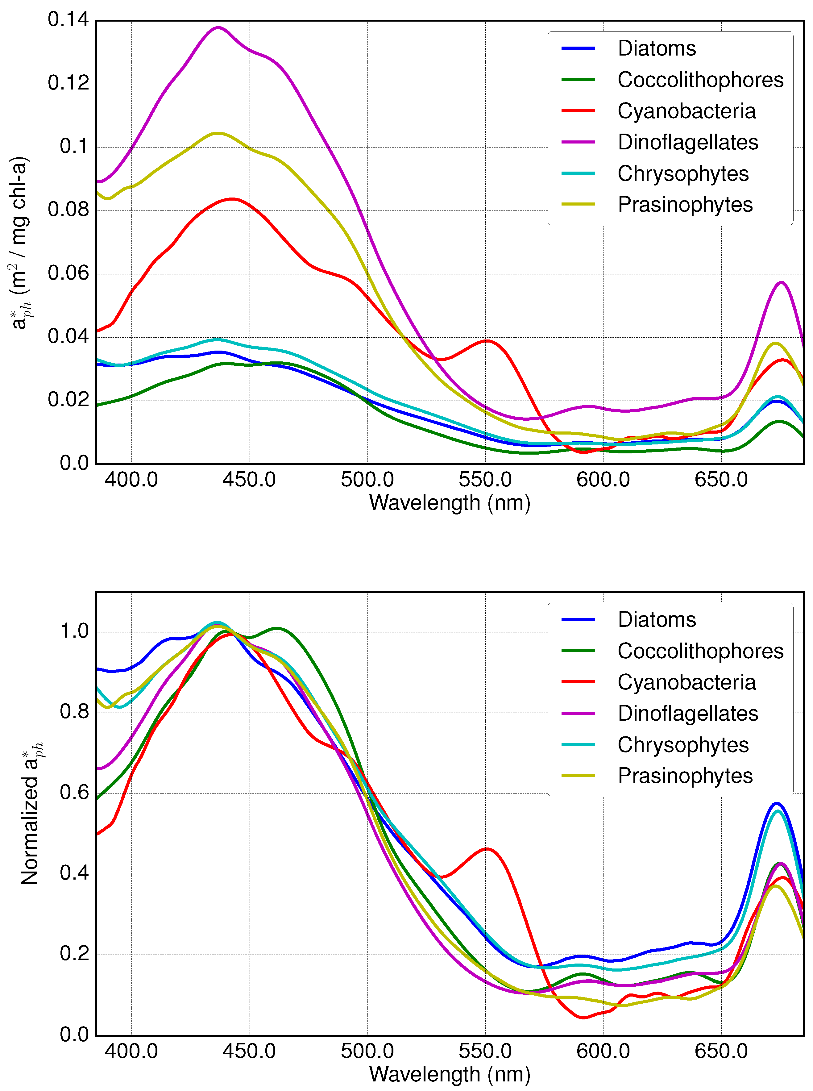
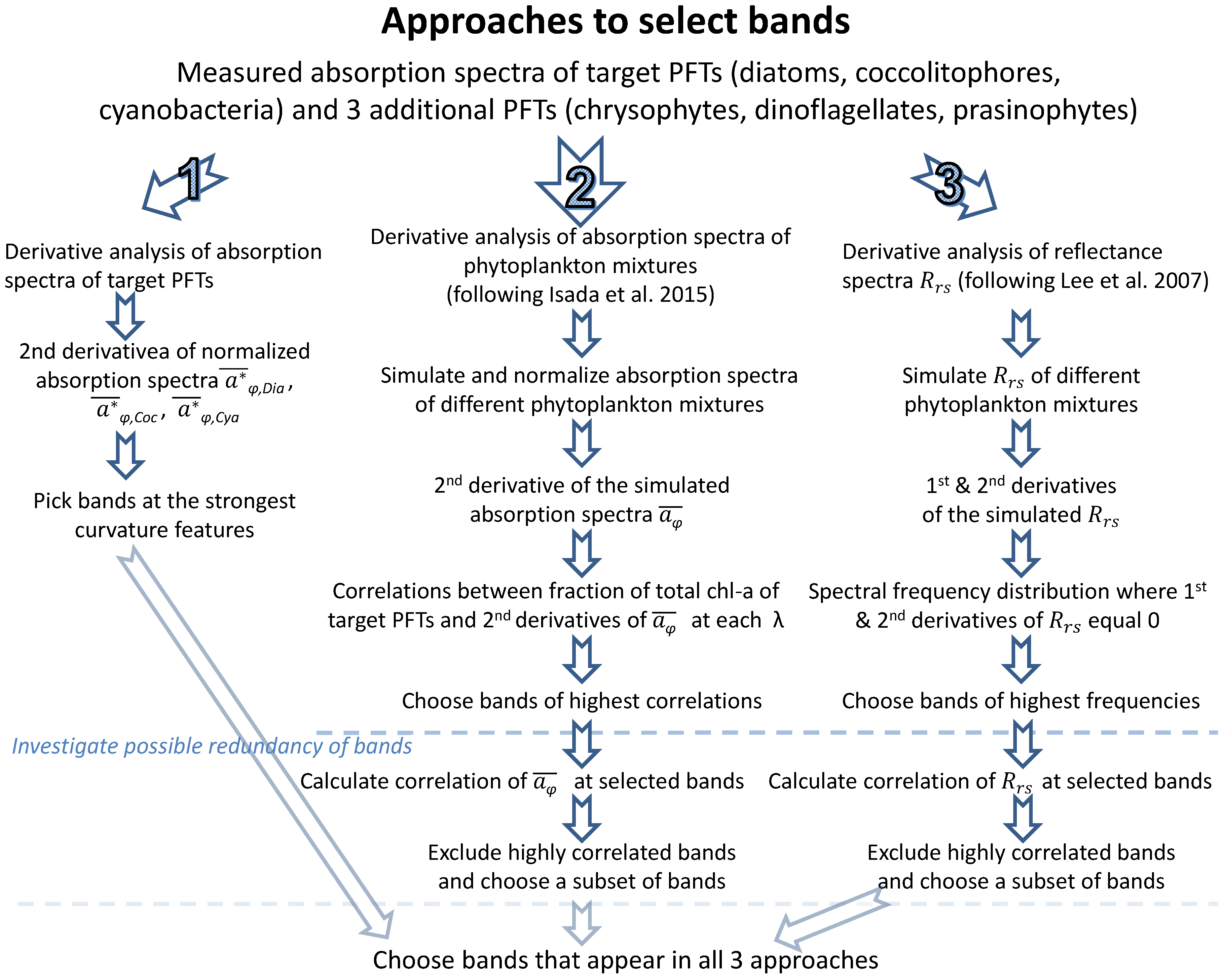
2.1. Absorption Spectra of PFTs

Diatoms, coccolithophores and cyanobacteria constitute the target PFTs of this study. The absorption spectra of diatoms and cyanobacteria, which were used in this study, were the same as in Bracher et al. [13]. These spectra were measured on surface water samples from two different cruises (Polarstern cruises ANTXXI/3 and ANTXXIII/1). The absorption spectrum of coccolithophores is the same as in Sadeghi et al. [14] and was acquired from an Emiliania huxleyi culture, which is the most abundant and widespread species of coccolithophores [17]. More information on the absorption spectra of diatoms and cyanobacteria can be found in Bracher et al. [13] and of coccolithophores in Sadeghi et al. [14].

Additionally, the absorption spectra of three non-target PFTs (dinoflagellates, chrysophytes and prasinophytes) were used to investigate how the inclusion of other PFTs influences the analysis of the absorption spectra of a mixed community (see Section 2.4 and Section 3.2). The absorption spectra of dinoflagellates and chrysophytes were measured during the MD OOMPH cruise using the point-source integrating-cavity absorption meter (PSICAM) technique [18], as described in [14]. The absorption spectra of dinoflagellates were measured in natural samples where dinoflagellates dominated the phytoplankton (92.4%), with the remaining community composed of chrysophytes (∼5.4%) and prasinophytes (∼2.1%). The absorption spectrum of chrysophytes was measured in a water sample where chrysophytes constituted 95.3% of the chl-a, and the remaining 4.7% was attributed to prasinophytes. The absorption spectrum of prasinophytes was measured also using the PSICAM during the ANT 23-1 cruise, as described in [13]. Prasinophytes constituted 97% of the water sample for the prasinophytes absorption spectrum.

For most of the cases, we chose to use the absorption spectra of natural samples since the pigmentation of cultures might differ from natural samples due to different environmental conditions, notably artificial light source and nutrient availability. The specific absorption spectrum from Emiliania huxleyi cultures, which is spectrally very similar to the specific absorption of measured natural samples, is the one exception. For more details, see [14].

Figure 2 (top panel) shows the original measured chlorophyll a (chl-a) specific absorption spectra of diatoms, coccolithophores, cyanobacteria, dinoflagellates, chrysophytes and prasinophytes ($a_{\varphi D}^{*}\left(\lambda \right)$, $a_{\varphi Coc}^{*}\left(\lambda \right)$, $a_{\varphi Cya}^{*}\left(\lambda \right)$, $a_{\varphi Dino}^{*}\left(\lambda \right)$, $a_{\varphi Chr}^{*}\left(\lambda \right)$, $a_{\varphi Pra}^{*}\left(\lambda \right)$). The corresponding spectra normalized to $a_{\varphi }^{*}\left(443\right)$ are presented in Figure 2 (bottom panel) (${\overline{a^{*}}}_{\varphi D}\left(\lambda \right)$, ${\overline{a^{*}}}_{\varphi Coc}\left(\lambda \right)$, ${\overline{a^{*}}}_{\varphi Cya}\left(\lambda \right)$, ${\overline{a^{*}}}_{\varphi Dino}\left(\lambda \right)$, ${\overline{a^{*}}}_{\varphi Chr}\left(\lambda \right)$, ${\overline{a^{*}}}_{\varphi Pra}\left(\lambda \right)$).

2.2. Forward Modeling of $R_{rs}$

Remote sensing reflectances ($R_{rs}\left(\lambda \right)$) were simulated in a simplified manner using an ocean reflectance model, which is also commonly used in its inverse form for retrieving inherent optical properties (IOPs) from measured $R_{rs}\left(\lambda \right)$. We adopted a form of an ocean reflectance inversion model that follows that described by and utilized in the generalized IOP (GIOP) model software [19]. The code of the GIOP model was adapted to include the absorption and backscattering spectra of three target PFTs. While we recognize that such an ocean reflectance model (ORM) has been utilized elsewhere, we will refer to it as GIOP throughout the remainder of this manuscript for convenience. The following steps illustrate the set-up of this forward modeling.

Inherent optical properties of absorption and backscattering of ocean waters are related to subsurface remote-sensing reflectances $r_{rs}\left(\lambda \right)$ following [20], as:

$$\begin{array}{cc}\hfill r_{rs}\left(\lambda \right)& =0.0949u\left(\lambda \right)+0.0794u{\left(\lambda \right)}^2,\hfill \\ \hfill u\left(\lambda \right)& =\frac{b_b\left(\lambda \right)}{a\left(\lambda \right)+b_b\left(\lambda \right)},\hfill \end{array}$$

(1)

where $b_b\left(\lambda \right)$ is the total backscattering coefficient (m${}^{-1}$) and $a\left(\lambda \right)$ is the total absorption coefficient (m${}^{-1}$). The subsurface values $r_{rs}\left(\lambda \right)$, are related to $R_{rs}\left(\lambda \right)$ following [21]:

$$r_{rs}\left(\lambda \right)=\frac{R_{rs}\left(\lambda \right)}{0.52+1.7R_{rs}\left(\lambda \right)}.$$

(2)

The total absorption coefficient is expanded as the sum of all absorbing components:

$$a\left(\lambda \right)=a_w\left(\lambda \right)+a_{dg}\left(\lambda \right)+a_{\varphi }\left(\lambda \right),$$

(3)

where the subscripts w, $dg$ and ϕ indicate contributions by water, colored dissolved organic matter (CDOM) + non-algal particles (NAP) and phytoplankton, respectively.

The contributions of CDOM and NAP to $a_{dg}\left(\lambda \right)$ have similar exponential spectral shapes, which suggests that these two components may share some common chromophores [22]. In addition, the $dg$ combination cannot currently be accurately decomposed into its two components using remote-sensing methods. Hence, to focus here on the differentiation of various PFTs, the $dg$ combination was considered as a single term in our simplified model. Total backscattering is expanded to:

$$b_b\left(\lambda \right)=b_{bw}\left(\lambda \right)+b_{bp}\left(\lambda \right),$$

(4)

where the subscripts w and p indicate contributions by water and particles, respectively.

Absorbing and backscattering components are further expressed as the products of their concentration-specific absorption and/or backscattering spectra (eigenvectors; $a^{*}\left(\lambda \right)$ for absorption and $b^{*}\left(\lambda \right)$ for backscattering) and their concentrations (eigenvalues; A for absorption and B for backscattering). The coefficients $a_w\left(\lambda \right)$ and $b_{bw}\left(\lambda \right)$ were assumed as in the default GIOP configuration ($a_w\left(\lambda \right)$ is taken from [23] and $b_{bw}\left(\lambda \right)$ is taken from [24]). Absorption of dissolved organic matter and non-algal particles $a_{dg}\left(\lambda \right)$ was expressed as follows:

$$a_{dg}\left(\lambda \right)=A_{dg}{a}_{dg}^{*}\left(\lambda \right)=a_{dg}\left(443\right)exp(-S_{dg}(\lambda -443)).$$

(5)

We varied the value of $a_{dg}\left(443\right)$ among simulations ($a_{dg}\left(443\right)$ equaled 0.01, 0.05, 0.1, 0.15 and 0.2). $S_{dg}$ was set to 0.02061 following Maritorena et al. [25].

Phytoplankton absorption $a_{\varphi }\left(\lambda \right)$ was constructed from the contributions by diatoms, coccolithophores and cyanobacteria:

$$a_{\varphi }\left(\lambda \right)=A_{\varphi }{a}_{\varphi }^{*}\left(\lambda \right)=A_{\varphi D}{a}_{\varphi D}^{*}\left(\lambda \right)+A_{\varphi Coc}{a}_{\varphi Coc}^{*}\left(\lambda \right)+A_{\varphi Cya}{a}_{\varphi Cya}^{*}\left(\lambda \right),$$

(6)

where the subscripts D, $Coc$ and $Cya$ indicate diatoms, coccolithophores and cyanobacteria, respectively. Chl-a specific absorption coefficients for diatoms, coccolithophores and cyanobacteria ($a_{\varphi D}^{*}\left(\lambda \right)$, $a_{\varphi Coc}^{*}\left(\lambda \right)$, $a_{\varphi Cya}^{*}\left(\lambda \right)$) are described in Section 2.1.

Similarly, backscattering by particles $b_{bp}\left(\lambda \right)$ was expanded to:

$$b_{bp}\left(\lambda \right)=B_{bp}{b}_{bp}^{*}\left(\lambda \right)=b_{bd}\left(\lambda \right)+B_{b\varphi D}{b}_{b\varphi D}^{*}\left(\lambda \right)+B_{b\varphi Coc}{b}_{b\varphi Coc}^{*}\left(\lambda \right)+B_{b\varphi Cya}{b}_{b\varphi Cya}^{*}\left(\lambda \right),$$

(7)

where subscripts d, D, $Coc$ and $Cya$ indicate non-algal particles (NAP), diatoms, coccolithophores and cyanobacteria, respectively. Eigenvalues $B_{b\varphi }$ for PFTs are the same as $A\varphi$, since they are also related to the concentration of each PFT.

Backscattering properties for the three PFTs were not measured simultaneously with their absorption properties. Hence, backscattering properties were adapted from different studies performed for similar species (Bricaud et al. [26] and Ahn et al. [27]). Backscattering of diatoms was assumed as for Chaetoceros lauderi [26]. This species is a representative diatom species with a large size (∼25 $\mathsf{\mu }$m) and low intracellular chlorophyll concentration. Backscattering of coccolithophores was taken from Ahn et al. [27], who measured backscattering for Emiliania huxleyi. Backscattering of cyanobacteria (specifically of Synechococcus sp.) was taken from Ahn et al. [27], as well.

The backscattering of PFTs was expressed as:

$$\begin{array}{c}\hfill B_{bD}{b}_{bD}^{*}\left(\lambda \right)=A_{\varphi D}{b}_{\varphi D}^{*}\left(590\right){(\frac{\lambda }{590})}^{{\eta }_{\varphi D}},\\ \hfill B_{bCoc}{b}_{bCoc}^{*}\left(\lambda \right)=A_{\varphi Coc}{b}_{b\varphi Coc}^{*}\left(555\right){(\frac{\lambda }{555})}^{{\eta }_{\varphi Coc}},\\ \hfill B_{bCya}{b}_{bCya}^{*}\left(\lambda \right)=A_{\varphi Cya}{b}_{b\varphi Cya}^{*}\left(555\right){(\frac{\lambda }{555})}^{{\eta }_{\varphi Cya}},\end{array}$$

(8)

where $b_{\varphi D}^{*}\left(590\right)$ = 0.22, $b_{b\varphi Coc}^{*}\left(555\right)$ = 0.219 $\times {10}^{-3}$, $b_{b\varphi Cya}^{*}\left(555\right)$ = 0.516 $\times {10}^{-3}$; ${\eta }_{\varphi D}$ and ${\eta }_{\varphi Coc}$ both equaled 0, since both PFTs are rather large cells, and ${\eta }_{\varphi Cya}$ = −1, which is in agreement with theoretical predictions for picoplankton.

Backscattering of non-algal particles is difficult to simulate because of the lack of knowledge about their size distribution and refractive index. Here, a constant background was used following the approaches of Brewin et al. [28] and Werdell et al. [9] (four different constant backgrounds in total).

Following Brewin fet al. [28], $b_{bd}\left(\lambda \right)$ was expressed as:

$$b_{bd}\left(\lambda \right)=b_{bd}\left(470\right){(\frac{\lambda }{470})}^{{\eta }_d}.$$

(9)

In the first applied parametrization, $b_{bd}\left(470\right)$ was set to 0.00068 and ${\eta }_d$ to −1.9 and in the second parametrization $b_{bd}\left(470\right)$ was set to 0.00049 and ${\eta }_d$ to −3.4 (following Table 3 in Brewin et al. [28]).

Following Werdell et al. [9], the backscattering was expressed as:

$$b_{bd}\left(\lambda \right)=0.01b_d\left(555\right){(\frac{\lambda }{555})}^{{\eta }_d},$$

(10)

where $b_d\left(555\right)$ was set to 0.1 or 0.2 and ${\eta }_d$ was set to −1 (Table 1 in Werdell et al. [9]).

Concentrations of chl-a for each PFT varied between 0 and 10 mg·m${}^{-3}$ (explicitly, 14 different concentrations were used: 0.0, 0.01, 0.03, 0.05, 0.08, 0.10, 0.30, 0.50, 0.80, 1.00, 3.00, 5.00, 8.00, 10.00 (mg·m${}^{-3}$)). We simulated $R_{rs}$ for all of the possible combinations of the given parameters, which adds up to 54,880 simulated $R_{rs}$ spectra (5 ($a_{dg}$) × 4 ($b_{bd}$) × 14 ($A_{\varphi D}$) × 14 ($A_{\varphi Coc}$) × 14 ($A_{\varphi Cya}$)). Simulated ranges of variables cover a broad range of conditions between the coastal and oceanic waters, excluding extremely absorbing and scattering waters, for which the specific algorithms are usually designed.

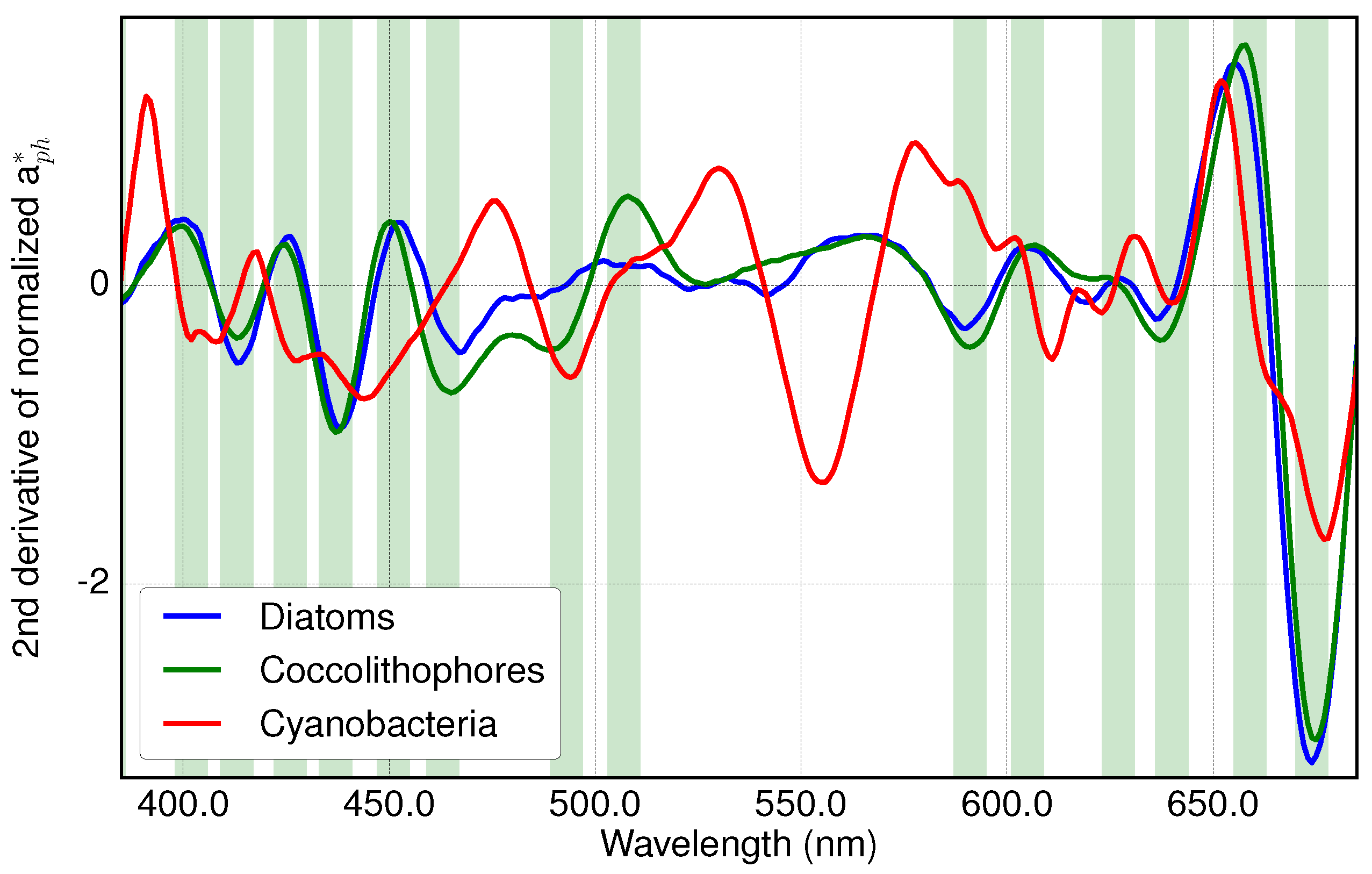
2.3. Derivative Analysis

Derivative analysis has been widely applied to analyze hyperspectral data of both inherent and apparent optical properties (e.g., [4,5,8,29,30]). It uses the first or higher order derivatives of spectral data to enhance small features within the spectra. Increasing derivative order leads to the suppression of the broad bands and increases the number of bands, which can be useful for identification of PFTs. However, the signal-to-noise ratios decreases as differentiation of higher orders is applied. Here, the derivative analysis was first applied directly to the absorption spectra of the target PFTs, but was also used in the further analysis of absorption and reflectance data based on studies of Isada et al. [5] and Lee et al. [4] (Section 2.4 and Section 2.5, respectively).

The first and second derivatives were calculated by finite difference approximation [29] using the following equations:

$$\begin{array}{cc}\hfill \frac{ds}{d\lambda }& \approx \frac{s(\lambda +\Delta \lambda )-s(\lambda -\Delta \lambda )}{2\Delta \lambda },\hfill \\ \hfill \frac{d^{2}s}{d^2\lambda }& \approx \frac{s(\lambda +\Delta \lambda )-2s\left(\lambda \right)+s(\lambda -\Delta \lambda )}{{(\Delta \lambda )}^2},\hfill \end{array}$$

(11)

where s is the spectrum used for the derivative transformation and $\Delta \lambda$ is the sampling interval. Since derivatives are sensitive to noise, mean filter smoothing was applied to the data beforehand with a filter window of 5, 9 or 10 nm, depending on the application. We followed precisely the choice of smoothing windows, as suggested by the studies, on which we based our analysis. Following [5], we used a smoothing window of 9 nm in the derivative analysis of absorption spectra. Nine nanometers was originally determined as the optimal value by [31], based on the sensitivity analysis of their second derivative spectra of phytoplankton absorption. In the derivative analysis of the reflectance spectra, we used the same filter window as in [4], who smoothed their measurements with a 5-nm running average. In addition, we also smoothed the spectra with a window double this size, 10 nm, which is also a typical bandwidth window for the satellite sensors. Smoothing windows of 9 nm and 10 nm are very similar, and in the case of the bands selected by different methods being 1 nm apart, we considered them being the same band identified by both methods.

In this first method, we looked for the spectral regions, which display the strongest features in the second derivatives of the absorption spectra of the target PFTs. The wavelengths of the maxima of spectral curvatures were chosen as candidate bands.

2.4. Application of Derivative Spectroscopy to Phytoplankton Absorption Spectra for Selection of Spectral Bands (Isada et al., 2015)

Isada et al. [5] examined the relationship between the concentration of phytoplankton community and the phytoplankton absorption spectra for the coastal waters of Funka Bay, Japan. They measured light absorption of phytoplankton (among other parameters) and calculated the contribution of various phytoplankton groups to the concentration of chl-a using HPLC pigment analysis by applying the CHEMTAX program. In total, 51 samples from surface waters were collected from April 2010–January 2012. They calculated the correlations between the concentration of three PFTs (diatoms, chlorophytes plus prasinophytes and cyanobacteria) and the second derivatives of the absorption spectra (normalized to absorption at 443 nm) at each wavelength from 400–700 nm. Fifteen wavelengths, which showed high correlations with each PFT, were suggested to improve the estimation of the phytoplankton community structure.

Here, we adapted their approach and applied it to simulated data (Figure 1). Different from the previous approach (Section 2.3), where we directly calculated the derivatives of the specific absorption spectra of the target PFTs, here we analyzed the absorption spectra of mixed phytoplankton communities. Phytoplankton absorption of different communities was calculated for the combinations of seven different concentrations (0, 0.01, 0.05, 0.1, 0.5, 1, 5 mg·m${}^{-3}$) of the three target and three non-target PFTs (117,649 scenarios), as the sum of the specific absorption spectra of each PFT multiplied by its concentration (the number of different concentrations is smaller here because of including three additional PFTs, which radically increases the number of scenarios). The spectra were then smoothed with a mean filter window of 9 nm (following [5] and [31]) and normalized to the absorption at 443 nm. Afterwards, second derivatives of the spectra were computed, following Equation (11).

The correlations between the concentration of the target PFTs (expressed in a fraction of the total chl-a) and second derivatives at each wavelength were first calculated considering only three target PFTs and, afterwards, all six PFTs. We also calculated correlations for scenarios of all PFTs, but excluding cyanobacteria, because cyanobacteria tended to dominate the calculated spectra (see Section 2.3). Packaging effects were not considered here, since we wanted to examine which wavelengths show the strongest linear correlation.

The wavelengths of highest correlations were compared with the spectral regions, which were previously chosen based on the derivative analysis of the specific measured PFT absorption spectra (Section 3.2). Furthermore, we calculated correlation coefficients for normalized absorption coefficients of the phytoplankton mixtures at each chosen wavelength with all other chosen wavelengths. Highly correlated bands indicated the potential redundancy of the measurements and the opportunity to reduce the number of selected bands.

2.5. Application of Derivative Spectroscopy to Reflectance Spectra for Selection of Spectral Bands (Lee et al., 2007)

Lee et al. [4] applied the derivative analysis to measured $R_{rs}$, to select optimal wavelengths for band placement. They calculated the first and second derivatives from nearly 400 hyperspectral measurements. The frequencies of zero (the number of zeros) values for these derivatives at each wavelength were counted, and the wavelengths with the highest frequency were selected as the potential location for band placement. They also calculated correlation coefficients between $R_{rs}$ at the suggested bands to indicate which adjacent bands could be potentially removed because of the redundancy.

We applied this approach to all modeled $R_{rs}$ (Figure 1), which were simulated as described in Section 2.2. Following [4], we selected the wavelengths with the highest frequencies of the first and second derivatives equaled to zero. Based on the correlation between $R_{rs}$ at the selected wavelengths, we also identified the potential redundancy of the spectral information.

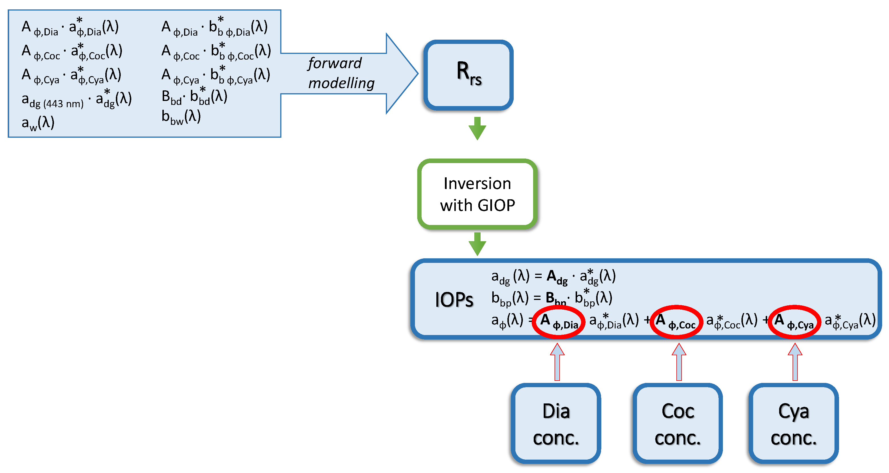
2.6. Ocean Reflectance Inversion with GIOP

We adapted the same model software GIOP, which was used for forward modeling (Section 2.2) to run the inversion and evaluate retrievals of PFTs based on certain band placements. The flowchart of the inversion is shown in Figure 3. Using $R_{rs}\left(\lambda \right)$ (simulated as described in Section 2.2), absorption and backscattering eigenvectors as input, eigenvalues for absorption (A) and backscattering (B) are estimated via nonlinear least squares inversion. GIOP software was adapted to solve additional absorbing phytoplankton components (three PFTs). $a_{\varphi }^{*}\left(\lambda \right)$ for each PFT is provided as chl-a specific absorptions, and the eigenvectors $A_{\varphi D}$, $A_{\varphi Coc}$, $A_{\varphi Cya}$ provide an estimate of chl-a concentration of diatoms, coccolithophores and cyanobacteria, respectively.

The simulated scenarios reflect the conditions where all absorption spectra are known, even though such information is very difficult to obtain for normal remote sensing retrievals. The retrieval followed the default configuration [19]. The ORM was applied to the simulated $R_{rs}\left(\lambda \right)$ using different suites of smoothing filters and input wavelengths of bands chosen in this study and three satellite instruments: Moderate Resolution Imaging Spectroradiometer (MODIS), Medium Resolution Imaging Spectrometer (MERIS), and Sea-Viewing Wide Field-of-View Sensor (SeaWIFS).

The input chl-a concentration data for the respective PFT in the simulation were used as the reference. The performance of each retrieval was evaluated by calculating the correlation coefficient (r) and mean absolute error ($MAE$) between the reference and retrieved values. $MAE$ was calculated as:

$$MAE=\frac{1}{n}\sum _{i=1}^n|x_{i,retrieved}-x_{i,reference}|,$$

(12)

where $x_{i,retrieved}$ and $x_{i,reference}$ are the retrieved chl-a and reference chl-a concentrations of the given PFT, respectively. The statistics were performed on the successful retrievals with retrieved chlorophyll concentration up to 50 mg·m${}^{-3}$.

3. Results

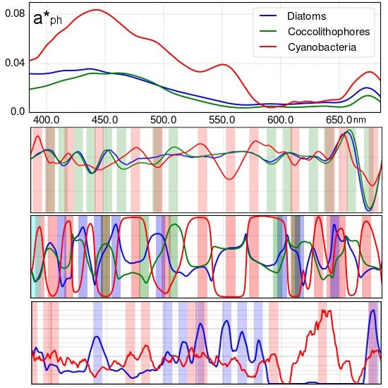
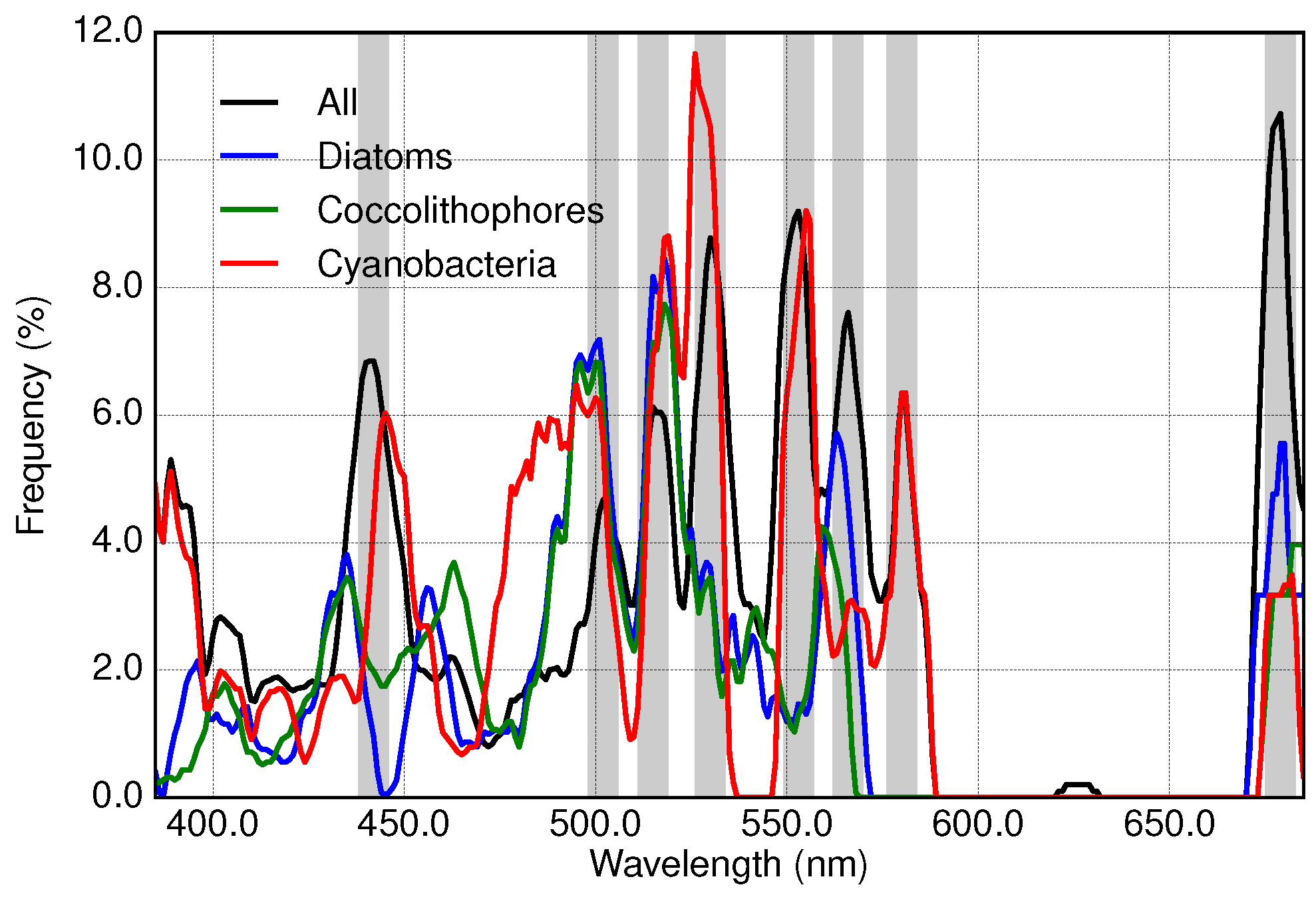
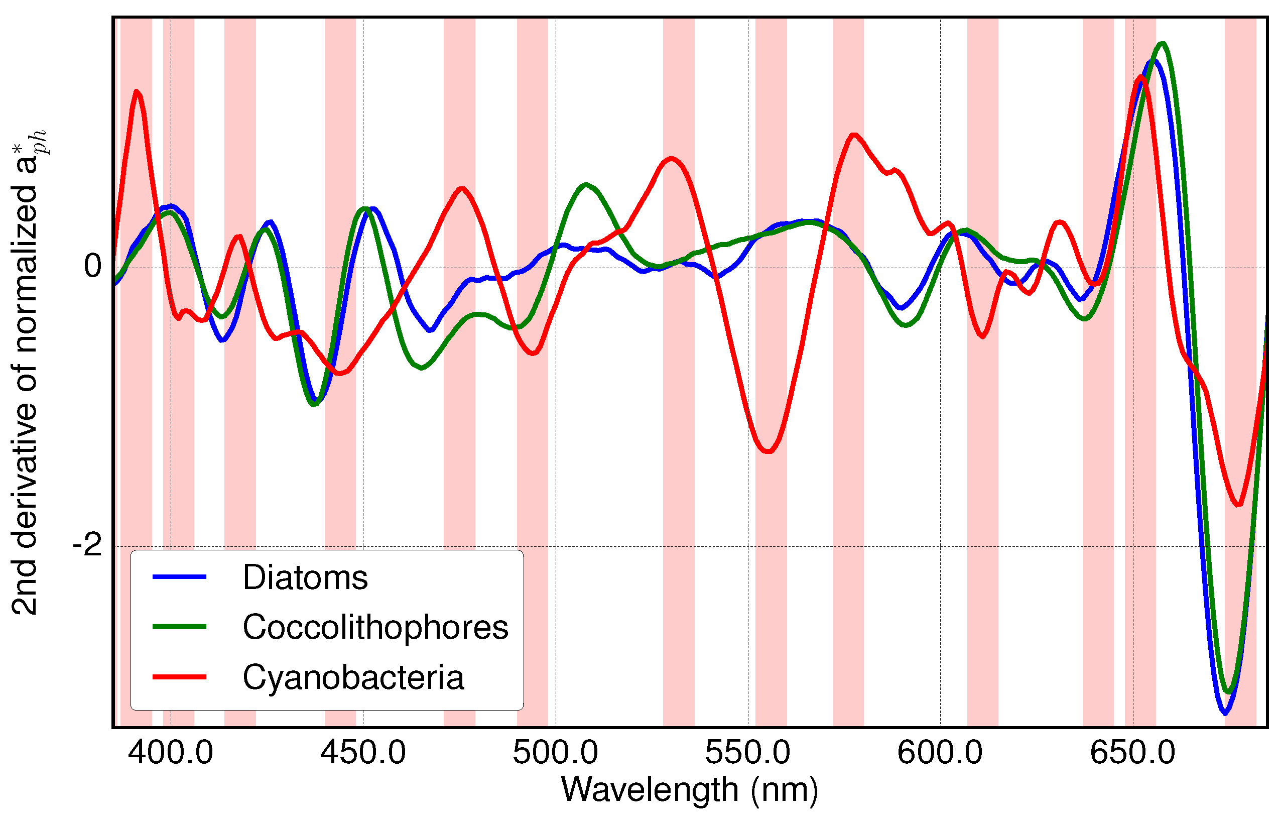
3.1. Analysis of Specific Measured PFT Absorption Spectra of Diatoms, Coccolithophores and Cyanobacteria Using Derivative Analysis

The second derivatives of ${\overline{a^{*}}}_{\varphi }\left(\lambda \right)$ for each target PFT are shown in Figure 4. The positions of the identified absorption peaks and valleys are indicated. Based on these spectra, wavelengths of maxima of spectral curvature were located. The ‘candidate’ bands for PFTs are highlighted in Figure 4 and given in

Table 1. Summary of the bands chosen by different approaches (spectral resolution of 10 nm) and the bands of the existing instruments. Abbreviations for the band settings are the same as in Table 2. Medium Resolution Imaging Spectrometer (MERIS) and Ocean and Land Colour Instrument (OLCI) bands are the same, with the exception of additional OLCI bands (400 nm and 674 nm) highlighted in red. Bands in color are the bands that were excluded in order to make a subset with a smaller number of bands. The bands that were removed from ‘Freq. 10 nm’ to ‘Freq. 10 nm red.’ are in green. In the case of ‘a${}_{\mathrm{ph}}^{*}$ devs’ sets, the bands removed from the original set ‘a${}_{\mathrm{ph}}^{*}$ devs’ to ‘a${}_{\mathrm{ph}}^{*}$ devs red.v.1’ are in green; the bands that were further removed to `a${}_{\mathrm{ph}}^{*}$ devs red.v.2’ are in red; and the bands finally removed to ‘a${}_{\mathrm{ph}}^{*}$ devs red.v.3’ are in blue.

a${}_{\mathbf{ph}}^{\mathbf{*}}$ Devs	a${}_{\mathbf{ph}}$ devs (+red.v.1,2,3)	Freq. 10 nm (+red.)	Mix	MERIS & OLCI	MODIS	SeaWIFS	H&S, 1991	Isada et al., 2015	Lee et al., 2007
		376
382	382	379	381
		386					384		385
391	390
	393								395
		399
402	404	405	404	400
413	412			412	412	412	413	411
418	418
426	430								425
437							435
444	443	442	443	443	443	443		433	440
451	449
463	458						461	458	460
475	475	470	473						475
	482	483
				490	488	490	490	488	490
493	496
494
	501	502
507	507			510		510		512	510
		515
		523
		530			531			531
532	532	532	532				532
									545
556	556	553	555		551	555		556
				560
		566							565
576	576	580	578				583	585	580
591	596	593	594					599
605	600
611	611
	612
	615			620			623	615	615
627	631	635	631					633	635
640
641	642
	645						644	646
652	650						655
				665	667	670		662	665
674	672			674				674
678		678
		679		681	678		676
									685
							700	694	710

(which summarizes bands selected with all approaches) as ‘a${}_{\mathrm{ph}}^{*}$ devs’ (a subset of bands chosen with the second derivatives analysis of spectra of each PFT). Since derivatives of the spectra of coccolithophores and diatoms indicate mostly very similar locations, bands attributed to them are grouped together (Figure 4, bottom panel). Cyanobacteria show more distinct features, which hence are indicated separately in the top panel of Figure 4.

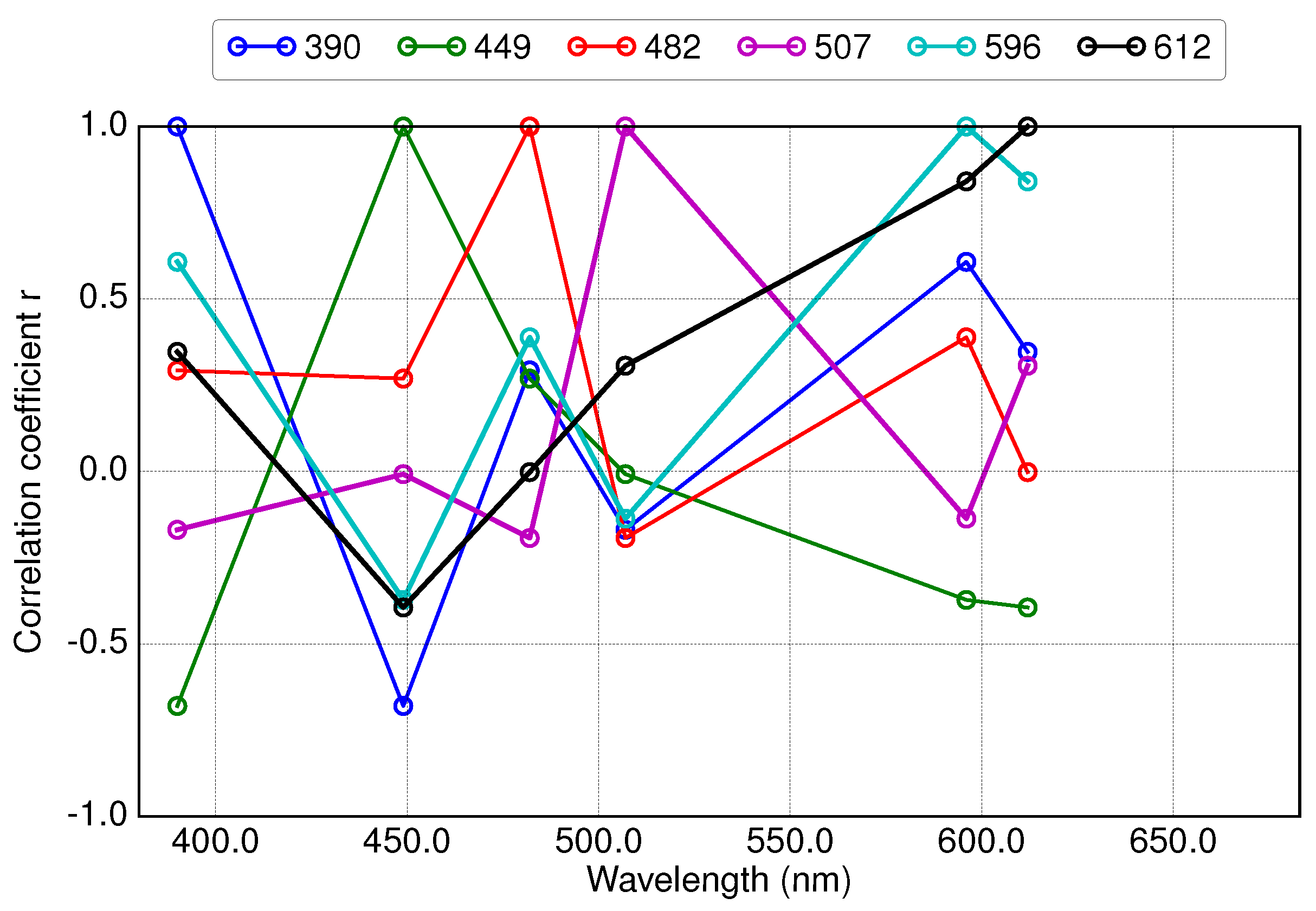
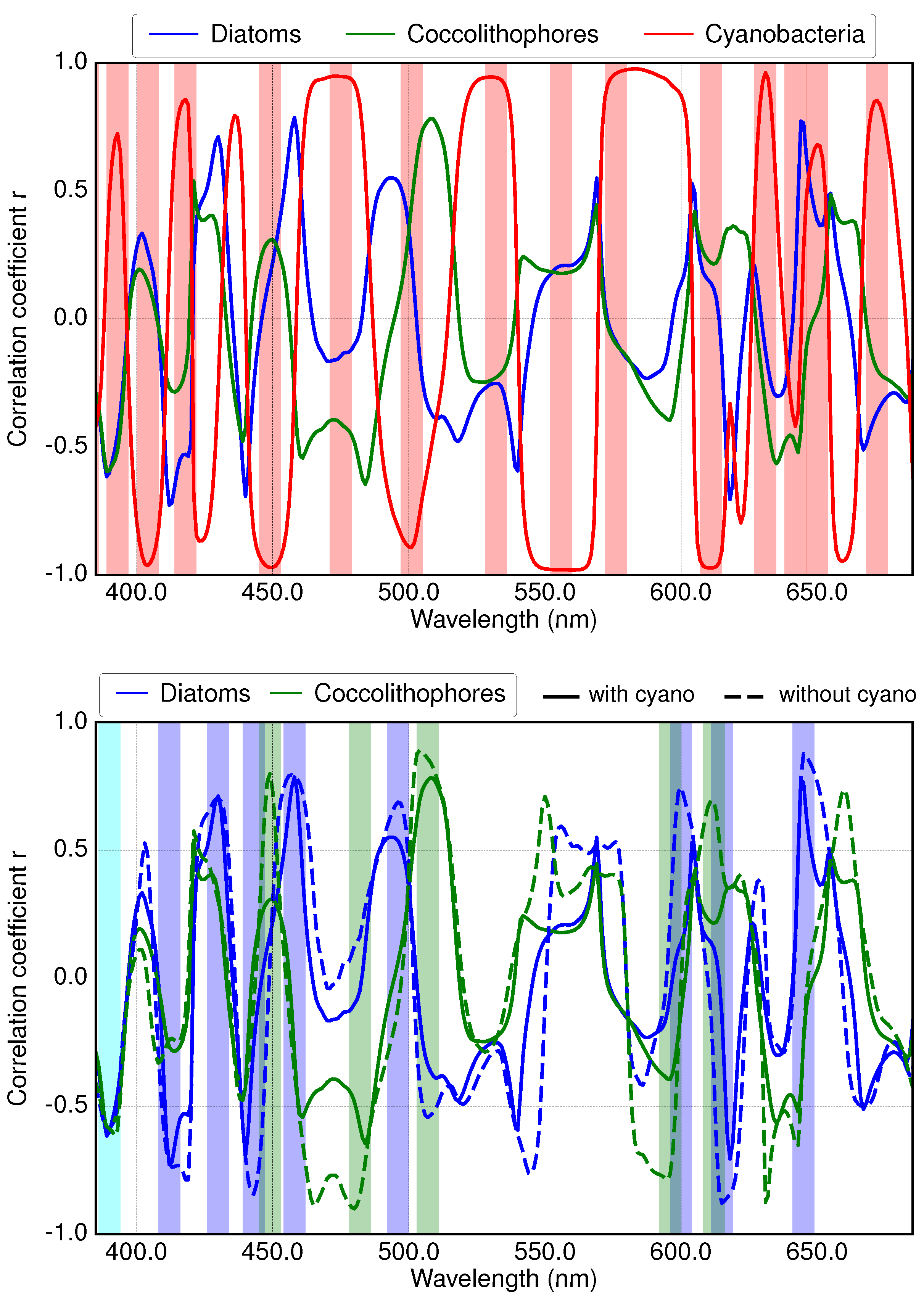
3.2. Results of Applying Derivative Spectroscopy to Mixtures of Phytoplankton Specific Absorption Spectra for the Selection of Spectral Bands, Following Isada et al., 2015

We calculated the correlations between the compositions of the target PFTs (expressed as a fraction of the total chl-a concentration) and second derivatives of the normalized absorption spectra of simulated mixtures at all wavelengths. When only the three target PFTs are considered in the mixtures, the calculated correlations reflect approximately the peaks as observed directly in the derivatives of the absorption spectra of each PFT (see Section 3.1). However, the separation between the maximal features for diatoms and coccolithophores is better visible here than in the derivative analysis of the previous section. To examine how these results are affected by including other PFTs in the mixture, the correlations were also calculated for the mixture of all six PFTs (Figure 5, top panel). In general, including other PFTs decreases the correlation coefficients of each PFT, and some of the features are smoothed or decreased as compared to when considering only three PFTs. Since the cyanobacteria has the highest amplitude of the PFT chl-a specific absorption spectrum and more spectral features related to additional specific pigments (specifically phycobilisomes, with absorption peaks around 493 nm and 556 nm; see Figure 2 and Figure 4), their features are dominating the correlations. Hence, for an additional comparison, cyanobacteria were excluded from phytoplankton mixtures (Figure 5, bottom panel). In such a case, correlations for diatoms and coccolithophores at all red wavelengths increase significantly. Certain peaks related to diatoms and coccolithophores (e.g., 550 nm) are suppressed if cyanobacteria are included in the simulations.

In Figure 5, we highlighted the bands that were chosen separately for cyanobacteria (top panel) and diatoms and coccolithophores (bottom panel). In the previous approach (Section 3.1), bands were simultaneously chosen for diatoms and coccolithophores, since their spectral features were not well separated.

To investigate the redundancy of spectral information, linear regression analysis of the normalized absorption spectra at the chosen wavelengths was carried out. For example, in the case of the bands chosen for coccolithophores, normalized absorption (of phytoplankton mixtures) at 390 nm, 449 nm, 482 nm, 507 nm, 596 nm and 612 nm were used as the independent variables. For each of them, correlations with all other chosen bands were calculated, which are shown in Figure 6. By excluding some of the highly correlated bands, we created an additional subset.

The chosen bands before excluding any of them are given in Table 1 as ‘a${}_{\mathrm{ph}}$ devs’ (a subset of bands chosen with the derivatives analysis of spectra of PFTs mixtures). By excluding highly correlated bands for each PFT, a reduced subset ‘a${}_{\mathrm{ph}}$ devs, red.v.1’ of them was chosen. Since the chosen bands were strongly dominated by bands chosen for cyanobacteria (which have multiple spectral features corresponding to phycobilisomes), for further comparison, we additionally reduced the number of bands by leaving only one band specific for cyanobacteria (‘a${}_{\mathrm{ph}}$ devs, red.v.2’) and by excluding all cyanobacteria-specific bands (‘a${}_{\mathrm{ph}}$ devs, red.v.3’).

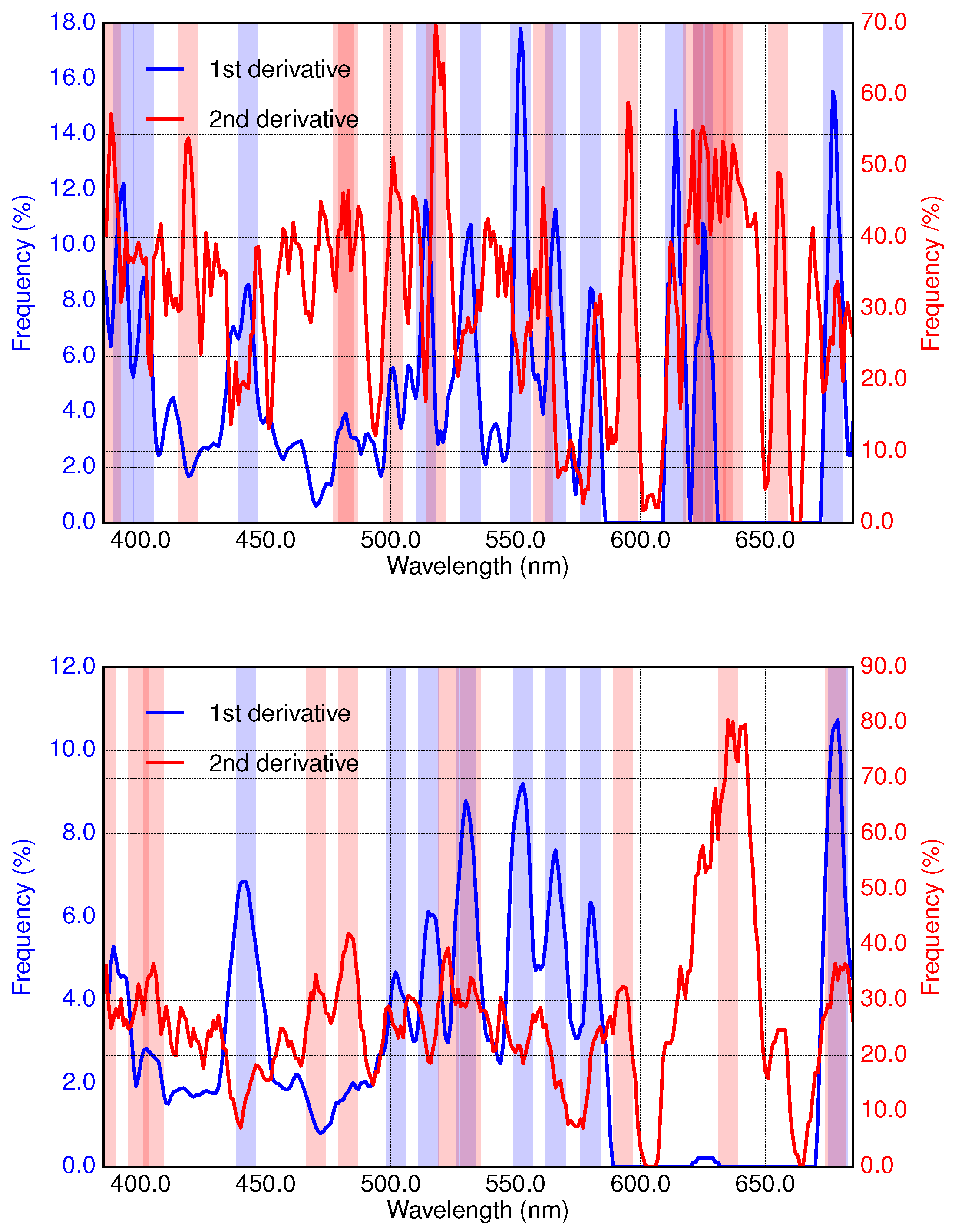
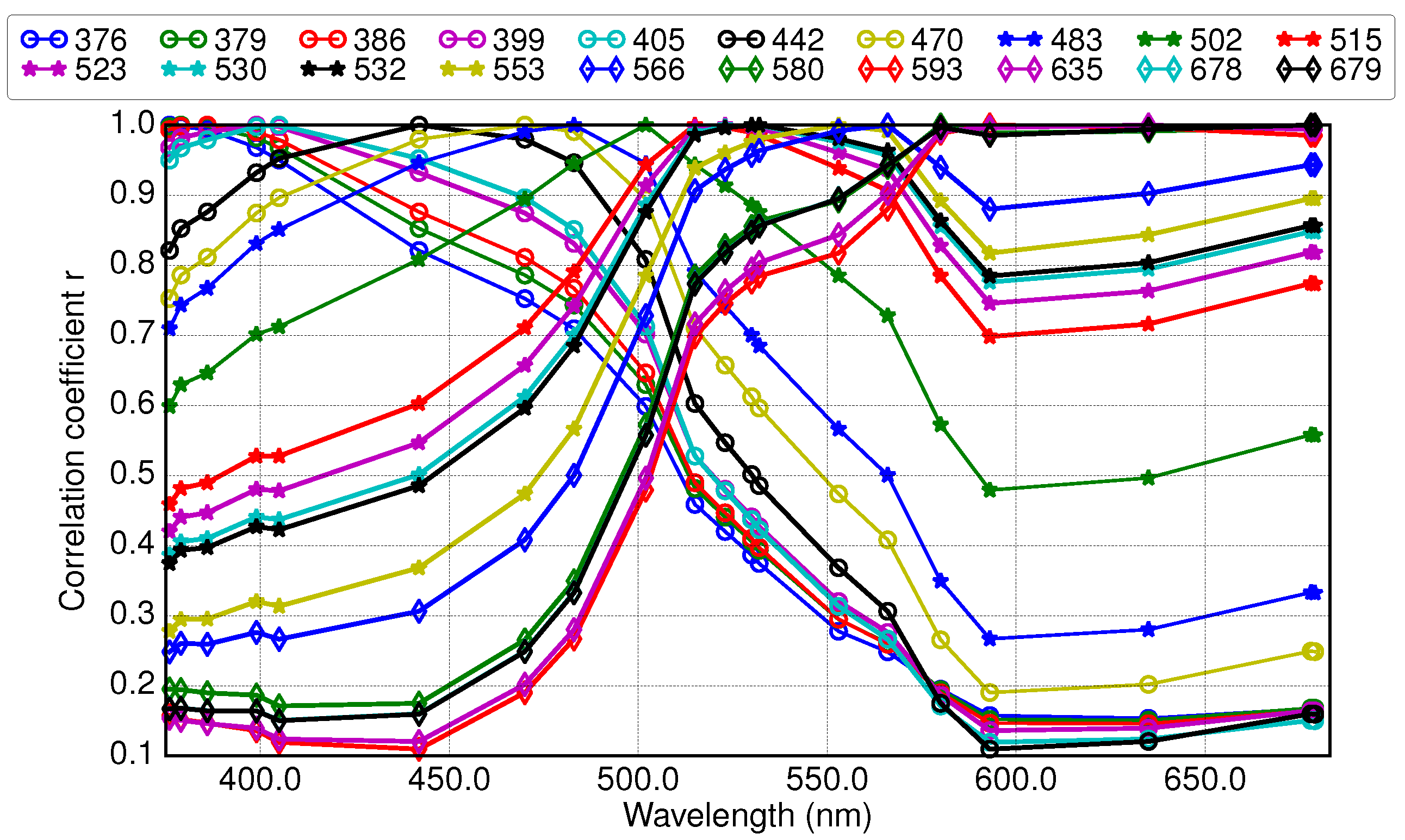
3.3. Results of Applying Derivative Spectroscopy to Reflectance Spectra for Selection of Spectral Bands, Following Lee et al., 2007

We calculated the spectral distribution of frequencies where first and second derivatives of simulated $R_{rs}$ spectra equaled zero for smoothing windows of 5 nm and 10 nm (Figure 7, top and bottom, respectively). Higher values correspond to more appearances of the derivatives crossing zero. The bands of the highest frequencies of zero crossing are highlighted and indicate possible placement of the satellite bands. Though some wavelengths indicate high frequencies only for smoothing with a smaller filter window (of 5 nm), many features coincide for both applied smoothings (5 nm or 10 nm).

In addition, we compared these spectral distributions of the first derivatives for each target PFT separately (Figure 8). By comparing the obtained distributions, it is possible to determine which PFT drives the high frequencies at a given wavelength. In this approach, again, cyanobacteria dominated the spectral features (shown by the highest frequencies).

The possible redundancy of bands was also investigated similarly to Section 3.2, by calculating correlation coefficients among the chosen bands for $R_{rs}$ (e.g., as shown in Figure 9 for a 10-nm smoothing window). From groups of bands that were highly correlated, only one band was chosen (for example, from bands at wavelengths of 376 nm, 379 nm and 386 nm, the band of 379 nm was chosen). The chosen bands for 10-nm resolution, before and after excluding highly correlated ones, are given in Table 1 as ‘Freq. 10 nm’ and ‘Freq. 10 nm red.’, respectively.

3.4. Results of GIOP Retrievals

The GIOP retrievals of diatoms, coccolithophores and cyanobacteria were tested on the different band placements as chosen in the Section 3.1, Section 3.2 and Section 3.3. An additional subset of similar wavelengths chosen in all three approaches (‘a${}_{\mathrm{ph}}^{*}$ devs’, ‘a${}_{\mathrm{ph}}$ devs, red.v.1’, ‘Freq. 10 nm, red.’) was also tested and is indicated as ‘Mix’ in Table 1, Table 2, Table 3 and Table 4. In addition, band locations of previous ocean color satellite sensors were included in the comparison. Since we wanted to focus on the location of the bands, and not their bandwidth (SeaWIFS, for example, has mostly bands with a bandwidth of 20 nm, while MODIS and MERIS mostly of 10 nm), we used the same average filter of 10 nm. In addition, we also tested continuous hyperspectral data with spectral sampling and resolutions of 1 nm, 5 nm, and 10 nm (as ‘All’ of the given resolution in Table 2, Table 3 and Table 4). Correlation coefficients (r) and mean absolute errors (MAE) calculated between the retrieved chl-a concentrations of each PFT and their input concentrations for diatoms, coccolithophores and cyanobacteria are shown in Table 2, Table 3 and Table 4, respectively.

The smallest values and largest variability of correlations among the different band placements was obtained for diatoms (Table 2). Additionally, MAE also varied the most for diatoms across all PFTs. The reduction of the number of bands (based on the correlation within the spectral bands) had a relatively small influence on the performance of the retrievals. Only when all cyanobacteria bands were excluded, the MAE increased significantly. Among the settings of the previous instruments, SeaWIFS had the highest r, while MERIS the smallest MAE. The performance of MODIS in this case was worse than MERIS and SeaWIFS.

For coccolithophores, the variability among the different scenarios was quite small and was larger for MAE than for r. Here, surprisingly, the removal of all cyanobacteria bands improved the performance of the retrieval as compared to the full set of bands. Here, the SeaWIFS was the best among the existing sensors.

The retrievals of cyanobacteria had the highest r and lowest MAE. This is expected, since they have the most distinctive features among the target PFTs. MAE and r were quite similar among the investigated band settings, with the exception of MAE ‘a${}_{\mathrm{ph}}$ devs, reduced v.2’ (where the specific bands of cyanobacteria were completely excluded) and MODIS and SeaWIFS, where the results were much worse. MERIS showed the best performance among the sensors and results close to the best approach.

Continuous hyperspectral data usually gave the best results for all three target PFTs, and they did not vary much among different resolutions.

4. Discussion

4.1. Band Placement Determined with Different Approaches

The variations of band placement, as determined by different approaches, are summarized in Table 1 (see the results in Section 3.1, Section 3.2 and Section 3.3). In addition, we also present the band placements, as determined with the original approaches that were adapted to simulated data for this study [4,5]. The bands from [3], to which both above-mentioned studies compared their own results, are also shown. For comparison, we added the bands of the multispectral ocean color instruments SeaWIFS, MODIS, MERIS and OLCI.

The first two approaches, which are both based on the derivative analysis of the absorption spectra of PFTs and phytoplankton mixtures (‘a${}_{\mathrm{ph}}^{*}$ devs’ and ‘a${}_{\mathrm{ph}}$ devs’ in Table 1) provide quite similar results. Bands of ‘a${}_{\mathrm{ph}}^{*}$ devs’, which were identified as the peaks in the spectra, were sometimes overlapping. The approach of ‘a${}_{\mathrm{ph}}$ devs’ was more successful in separating features of diatoms and coccolithophores, but at the same time, the maxima of correlations were broader, which made it more difficult to choose the exact bands.

Many bands showed up in all three adapted techniques (‘a${}_{\mathrm{ph}}^{*}$’, ‘a${}_{\mathrm{ph}}$’ and ‘Freq. 10 nm’), which was expected since in all of them, we used the same absorption spectra of PFTs. However, sometimes, some bands were obtained only for one of the analyses. In general, larger differences were obtained for the set ‘Freq. 10 nm’, as it was using reflectance and not absorption data. Very often, bands were a little bit shifted from each other, which could be explained by using different kinds of data (absorption or reflectance) and different smoothing windows. In addition, the features that were common for diatoms and coccolithophores in the ‘a${}_{\mathrm{ph}}^{*}$’ approach were separated by a few nm in the ‘a${}_{\mathrm{ph}}$ devs’ approach, while features of cyanobacteria were much broader, and choosing the bands position was more flexible. By consolidating the bands that were common for all approaches (e.g., 381 nm, 404 nm, 443 nm, etc.), we made an additional subset, mix, shown also in Table 1.

It is interesting to note that some of the bands that were identified in our study (e.g., 385 nm, 412 nm, 443 nm, 530 nm, etc.), were also identified in previous studies of [4,5], despite using completely different datasets. In general, many bands also cover the same center wavelengths of the major pigments (e.g., 413 nm for chl-a and 532 nm for carotenoids), as identified by [3]. Most of the bands identified by our and previous studies (e.g., 412 nm, 443 nm, 510 nm, 531 nm) are also typically used in the ocean color satellite instruments. However, the bands at 490 nm (or 488 nm) and 620 nm were not selected by any of the methods here, which might be due to the fact that we focused here on the three specific PFTs, while these bands have been chosen in the past for ocean color remote sensing primarily of the pigment absorption in Case-2 waters and diffuse attenuation coefficient, and the total suspended matter, respectively. Our results can be used to select additional bands for future satellite sensors. In the case of OLCI, we would suggest adding four bands at 381 nm, 532 nm, 594 nm and 473 nm or 631 nm (when considering improving retrievals of diatoms, coccolithophores and cyanobacteria), which corresponds to the bands of the mix subset. This might be possible by changing the configuration of future OLCI instruments (e.g., Sentinel-C, -D, etc.).

In general, we observe a high level of consistency between the bands chosen by various approaches. The observed small diversity can arise from using various approaches and datasets. Even though we used the same specific absorption spectra of PFTs, we obtained quite a lot of variability within our approaches depending on the method applied. Hence, we conclude that it is not only the dataset, but the methods too, that can lead to different conclusions. Therefore, the method applied to determine the band placement is also a matter of choice in the first place, and the exact future application of the suggested bands (e.g., band ratios or inverse modeling) should also be taken into consideration, for example, by running designed retrievals on the simulated data.

4.2. Performance of GIOP Retrievals

As suggested above, we tested the chosen bands with the GIOP retrieval. We used the simplified scenarios, which was sufficient for the scope of this study. We do not claim that GIOP is the best possible method to retrieve PFTs, but it is indeed one of the possible solutions.

We compared the performance of the retrievals of diatoms, coccolithophores and cyanobacteria in Table 2, Table 3 and Table 4. In general, no single band placement led to the best GIOP retrievals for all PFTs. Although the set, for which most of cyanobacteria bands were excluded, led to an apparent worsening of the results of the retrievals of diatoms and cyanobacteria (from ‘a${}_{\mathrm{ph}}$ devs’ to ‘a${}_{\mathrm{ph}}$ devs’ red v.2), most of the different band placements scenarios performed very similarly. This suggests that at least one band was necessary for accurate differentiation between diatoms and coccolithophores. In general, the performed reduction of the number of bands (based on the correlation within the spectra) did not worsen the performance significantly, even though a large number of bands was removed (up to 50%). This supports the idea that some highly correlated bands carry redundant information and can be removed, with only a small impact on the outcome. The correlation coefficients obtained here are quite high, but the obtained MAE are also quite large, despite simplified modeling and an excellent description of the optical parameters. This supports suggestions by [9,10] that it is difficult to obtain the qualitative concentrations of PFTs as retrieved with GIOP (and probably other spectral fitting inversions).

Among the sensors, MERIS gave the best results among the investigated instruments for diatoms and cyanobacteria, but SeaWIFS performed better for coccolithophores. Among all of the tested bands, the continuous hyperspectral data usually yielded the best results. A small improvement was obtained for increasing the resolution of hyperspectral from 10 nm to 5 nm, but no significant improvement was obtained for increasing resolution from 5 nm to 1 nm.

5. Summary and Conclusions

Three different methods were applied to examine the best placement of spectral bands to retrieve different PFTs from satellite remote sensing. Furthermore, the number of bands was reduced based on the correlation within the spectra, which did not worsen the performance significantly. In general, the three methods applied selected mostly similar bands, but the choice also deviated for some bands. This shows that the choice of band settings is mainly driven by the optical signatures of the target, but is further influenced also by the chosen method to determine band placements, as well as by the internal variability within the investigated dataset. The chosen band placements were evaluated by applying an adapted GIOP retrieval of the three target PFTs. The performance of the continuous hyperspectral data usually gave the best results (which did not vary much among different resolutions). This supports the strong recommendation of using continuous hyperspectral satellite data in the future. In order to improve retrievals of PFTs with multispectral data by adding specific bands, the band placement would depend on the specific target PFT, since no single band placement led to the best retrievals for all PFTs. In the case of OLCI with the nine spectral bands, an additional four bands are suggested for improving PFT retrievals.

References

1. Sathyendranath, S.; Aiken, J.; Alvain, S.; Barlow, R.; Bouman, H.; Bracher, A.; Brewin, R.; Bricaud, A.; Brown, C.W.; Ciotti, A.M.; et al. Phytoplankton Functional Types from Space; Reports of the International Ocean Colour Coordinating Group; International Ocean Colour Coordinating Group: Dartmouth, NS, Canada, 2014. [Google Scholar]
2. Le Quéré, C.; Harrison, S.P.; Colin Prentice, I.; Buitenhuis, E.T.; Aumont, O.; Bopp, L.; Claustre, H.; Cotrim Da Cunha, L.; Geider, R.; Giraud, X.; et al. Ecosystem dynamics based on plankton functional types for global ocean biogeochemistry models. Glob. Chang. Biol. 2005, 11, 2016–2040. [Google Scholar]
3. Hoepffner, N.; Sathyendranath, S. Effect of pigment composition on absorption properties of phytoplankton. Mar. Ecol. Prog. Ser. 1991, 73, l–23. [Google Scholar] [CrossRef]
4. Lee, Z.; Carder, K.; Arnone, R.; He, M. Determination of primary spectral bands for remote sensing of aquatic environments. Sensors 2007, 7, 3428–3441. [Google Scholar] [CrossRef]
5. Isada, T.; Hirawake, T.; Kobayashi, T.; Nosaka, Y.; Natsuike, M.; Imai, I.; Suzuki, K.; Saitoh, S.I. Hyperspectral optical discrimination of phytoplankton community structure in Funka Bay and its implications for ocean color remote sensing of diatoms. Remote Sens. Environ. 2015, 159, 134–151. [Google Scholar] [CrossRef]
6. Guanter, L.; Kaufmann, H.; Segl, K.; Foerster, S.; Rogass, C.; Chabrillat, S.; Kuester, T.; Hollstein, A.; Rossner, G.; Chlebek, C.; et al. The EnMAP spaceborne imaging spectroscopy mission for earth observation. Remote Sens. 2015, 7, 8830–8857. [Google Scholar] [CrossRef]
7. Del Castillo, C.E. Pre-Aerosol, Clouds, and ocean Ecosystem (PACE) Mission science definition team report. In Proceedings of the Ocean Carbon and Biogeochemistry Workshop, Woods Hole, MA, USA, 16–19 July 2012.
8. Xi, H.; Hieronymi, M.; Röttgers, R.; Krasemann, H.; Qiu, Z. Hyperspectral differentiation of phytoplankton taxonomic groups: A comparison between using remote sensing reflectance and absorption spectra. Remote Sens. 2015, 7, 14781–14805. [Google Scholar] [CrossRef]
9. Werdell, P.J.; Roesler, C.S.; Goes, J.I. Discrimination of phytoplankton functional groups using an ocean reflectance inversion model. Appl. Opt. 2014, 53, 4833–4849. [Google Scholar] [CrossRef] [PubMed]
10. Werdell, P.J.; Roesler, C.S.; Goes, J.I. Remotely searching for noctiluca miliaris in the Arabian Sea. In Proceedings of the 22th Ocean Optics Conference, Portland, ME, USA, 27–31 October 2014.
11. Burrows, J.P.; Hölzle, E.; Goede, A.P.H.; Visser, H.; Fricke, W. SCIAMACHY—Scanning imaging absorption spectrometer for atmospheric chartography. Acta Astronaut. 1995, 35, 445–451. [Google Scholar] [CrossRef]
12. Bovensmann, H.; Burrows, J.P.; Buchwitz, M.; Frerick, J.; Noël, S.; Rozanov, V.V.; Chance, K.V.; Goede, A.P.H. SCIAMACHY: Mission objectives and measurement modes. J. Atmos. Sci. 1999, 56, 127–150. [Google Scholar] [CrossRef]
13. Bracher, A.; Vountas, M.; Dinter, T.; Burrows, J.P.; Röttgers, R.; Peeken, I. Quantitative observation of cyanobacteria and diatoms from space using PhytoDOAS on SCIAMACHY data. Biogeosciences 2009, 6, 751–764. [Google Scholar] [CrossRef]
14. Sadeghi, A.; Dinter, T.; Vountas, M.; Taylor, B.B.; Altenburg-Soppa, M.; Peeken, I.; Bracher, A. Improvement to the PhytoDOAS method for identification of coccolithophores using hyper-spectral satellite data. Ocean Sci. 2012, 8, 1055–1070. [Google Scholar] [CrossRef] [Green Version]
15. Dinter, T.; Rozanov, V.V.; Burrows, J.P.; Bracher, A. Retrieving the availability of light in the ocean utilising spectral signatures of vibrational Raman scattering in hyper-spectral satellite measurements. Ocean Sci. 2015, 11, 373–389. [Google Scholar] [CrossRef] [Green Version]
16. Wolanin, A.; Rozanov, V.; Dinter, T.; Noël, S.; Vountas, M.; Burrows, J.; Bracher, A. Global retrieval of marine and terrestrial chlorophyll fluorescence at its red peak using hyperspectral top of atmosphere radiance measurements: Feasibility study and first results. Remote Sens. Environ. 2015, 166, 243–261. [Google Scholar] [CrossRef] [Green Version]
17. Tyrrell, T.; Merico, A. Overview of fluorescence protocols: Theory, basic concepts, and practice. In Coccolithophores: From Molecular Processes to Global Impact; Thierstein, H.R., Young, J.R., Eds.; Springer: Berlin/Heidelberg, Germany, 2004; pp. 75–97. [Google Scholar]
18. Röttgers, R.; Schönfeld, W.; Kipp, P.R.; Doerffer, R. Practical test of a point-source integrating cavity absorption meter: the performance of different collector assemblies. Appl. Opt. 2005, 44, 5549–5560. [Google Scholar] [CrossRef] [PubMed]
19. Werdell, P.J.; Franz, B.A.; Bailey, S.W.; Feldman, G.C.; Boss, E.; Brando, V.E.; Dowell, M.; Hirata, T.; Lavender, S.J.; Lee, Z.; et al. Generalized ocean color inversion model for retrieving marine inherent optical properties. Appl. Opt. 2013, 52, 2019–2037. [Google Scholar] [CrossRef] [PubMed]
20. Gordon, H.R.; Brown, O.B.; Evans, R.H.; Brown, J.W.; Smith, R.C.; Baker, K.S.; Clark, D.K. A semianalytic radiance model of ocean color. J. Geophys. Res. 1988, 93, 10909–10924. [Google Scholar] [CrossRef]
21. Lee, Z.; Carder, K.L.; Arnone, R.A. Deriving inherent optical properties from water color: A multiband quasi-analytical algorithm for optically deep waters. Appl. Opt. 2002, 41, 5755–5772. [Google Scholar] [CrossRef] [PubMed]
22. Babin, M. Variations in the light absorption coefficients of phytoplankton, nonalgal particles, and dissolved organic matter in coastal waters around Europe. J. Geophys. Res. 2003. [Google Scholar] [CrossRef]
23. Pope, R.M.; Fry, E.S. Absorption spectrum (380–700 nm) of pure water. II. Integrating cavity measurements. Appl. Opt. 1997, 36, 8710–8723. [Google Scholar] [CrossRef] [PubMed]
24. Smith, R.C.; Baker, K.S. Optical properties of the clearest natural waters (200–800 nm). Appl. Opt. 1981, 20, 177–184. [Google Scholar] [CrossRef] [PubMed]
25. Maritorena, S.; Siegel, D.; Peterson, A. Optimization of a semianalytical ocean color model for global-scale applications. Appl. Opt. 2002, 41, 2705–2714. [Google Scholar] [CrossRef] [PubMed]
26. Bricaud, A.; Bédhomme, A.L.; Morel, A. Optical properties of diverse phytoplanktonic species: Experimental results and theoretical interpretation. J. Plankton Res. 1988, 10, 851–873. [Google Scholar] [CrossRef]
27. Ahn, Y.H.; Bricaud, A.; Morel, A. Light backscattering efficiency and related properties of some phytoplankters. Deep Sea Res. A Oceanogr. Res. Pap. 1992, 39, 1835–1855. [Google Scholar] [CrossRef]
28. Brewin, R.J.; Dall’Olmo, G.; Sathyendranath, S.; Hardman-Mountford, N.J. Particle backscattering as a function of chlorophyll and phytoplankton size structure in the open-ocean. Opt. Express 2012, 20, 17632–17652. [Google Scholar] [CrossRef] [PubMed]
29. Tsai, F.; Philpot, W. Derivative analysis of hyperspectral data. Remote Sens. Environ. 1998, 66, 41–51. [Google Scholar] [CrossRef]
30. Torrecilla, E.; Piera, J.; Vilaseca, M. Derivative analysis of hyperspectral oceanographic data. In Advances in Geoscience and Remote Sensing; Jedlovec, G., Ed.; InTech Open Access Publisher: Rijeka, Croatia, 2009; pp. 597–618. [Google Scholar]
31. Torrecilla, E.; Stramski, D.; Reynolds, R.A.; Millán-Núñez, E.; Piera, J. Cluster analysis of hyperspectral optical data for discriminating phytoplankton pigment assemblages in the open ocean. Remote Sens. Environ. 2011, 115, 2578–2593. [Google Scholar] [CrossRef] [Green Version]
Figure 1. Flowchart showing the three different approaches to select bands for phytoplankton functional type (PFT) retrievals and the fourth selection method based on all three methods.
Remotesensing 08 00871 g001
Figure 2. Measured chl-a specific (top) and normalized to 443 nm (bottom) absorption spectra ( a ϕ * ( λ ) and a * ¯ ϕ ( λ ) ) of diatoms, coccolithophores, cyanobacteria, dinoflagellates, chrysophytes and prasinophytes.
Remotesensing 08 00871 g002
Figure 3. Flowchart showing the inversion performed with GIOP.
Remotesensing 08 00871 g003
Figure 4. The second derivatives of a * ¯ ϕ ( λ ) for each target PFT. Both the top and bottom panels show the same spectra, but the chosen wavelengths are highlighted separately for cyanobacteria (top) and diatoms and coccolithophores (bottom).
Remotesensing 08 00871 g004aRemotesensing 08 00871 g004b
Figure 5. Correlation coefficients between the chl-a concentration of diatoms, coccolithophores and cyanobacteria and the second derivative spectra of normalized absorption coefficients of simulated mixtures. Highlighted areas indicate recommended spectral bands: red for cyanobacteria (top), blue and green for diatoms and coccolithophores, respectively (bottom). The color of the most left band in the bottom panel arises from the overlapping of both green and blue bands.
Remotesensing 08 00871 g005
Figure 6. Correlation coefficients of normalized absorption coefficients of simulated mixtures ( a * ¯ ϕ ( λ ) ) at wavelengths chosen for coccolithophores (highest correlation of second derivatives of a * ¯ ϕ ( λ ) at these wavelengths and chl-a concentration of coccolithophores); a * ¯ ϕ ( λ ) at each band indicated in the legend was used as the independent variable, respectively, while a * ¯ ϕ ( λ ) at other bands was considered as the dependent variable. A correlation coefficient for linear regression was then calculated for each a * ¯ ϕ ( λ ) pair.
Remotesensing 08 00871 g006
Figure 7. Spectral distribution of the frequency where the first and the second derivatives of simulated R r s equal zero for filter smoothing windows of 5 nm (top) and 10 nm (bottom). The bands of highest frequencies of the first and the second derivatives are highlighted in blue and red, respectively.
Remotesensing 08 00871 g007
Figure 8. Spectral distribution of the frequency where the first derivatives of simulated R r s equal zero (a filter smooth window of 10 nm) calculated for all the scenarios (black); and cases of including only diatoms (blue), coccolithophores (green) or cyanobacteria (red) in the simulations. Chosen regions of high frequencies are highlighted.
Remotesensing 08 00871 g008
Figure 9. Correlation coefficients among the chosen bands for R r s for 10 nm.
Remotesensing 08 00871 g009