
The Potential of Pan-Sharpened EnMAP Data for the Assessment of Wheat LAI

Abstract
:
1. Introduction
- (1)
- To prove the spatial enhancement as well as the spectral preservation capability of pan-sharpening when applied to hyperspectral EnMAP data.
- (2)
- To investigate the potential of the fusion results for a precise spatial intra-field assessment of wheat LAI for precision agriculture applications.
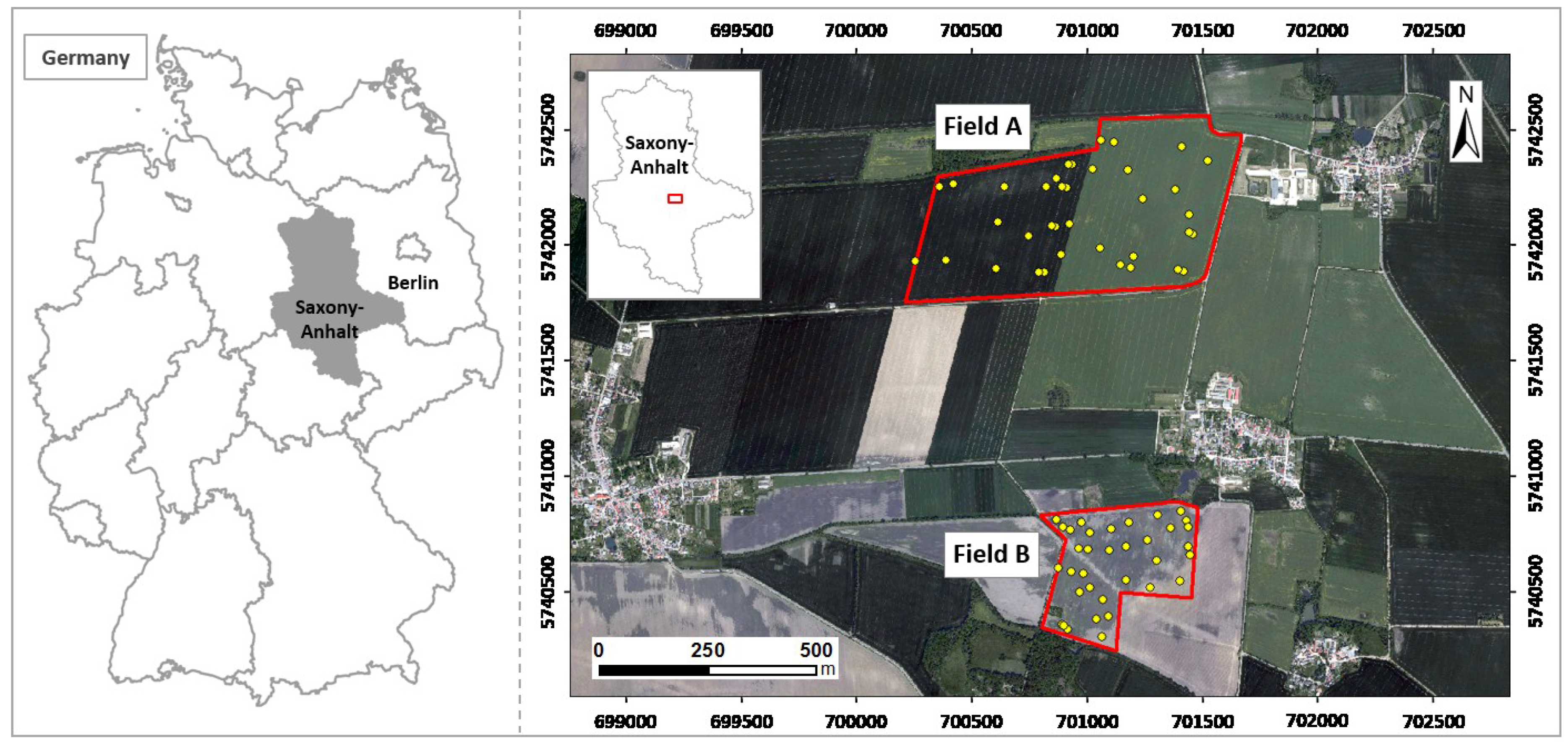
2. Study Area
3. Data and Pre-Processing
3.1. Field Data
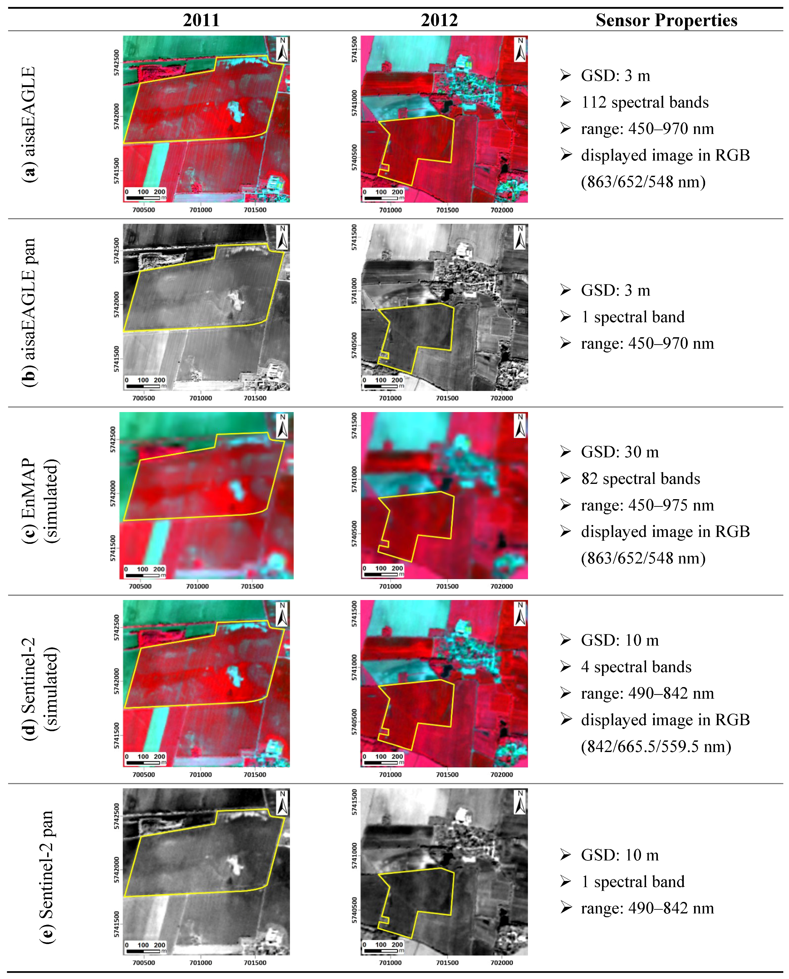
3.2. Airborne Data
3.3. Simulated Satellite-Data
4. Methodology
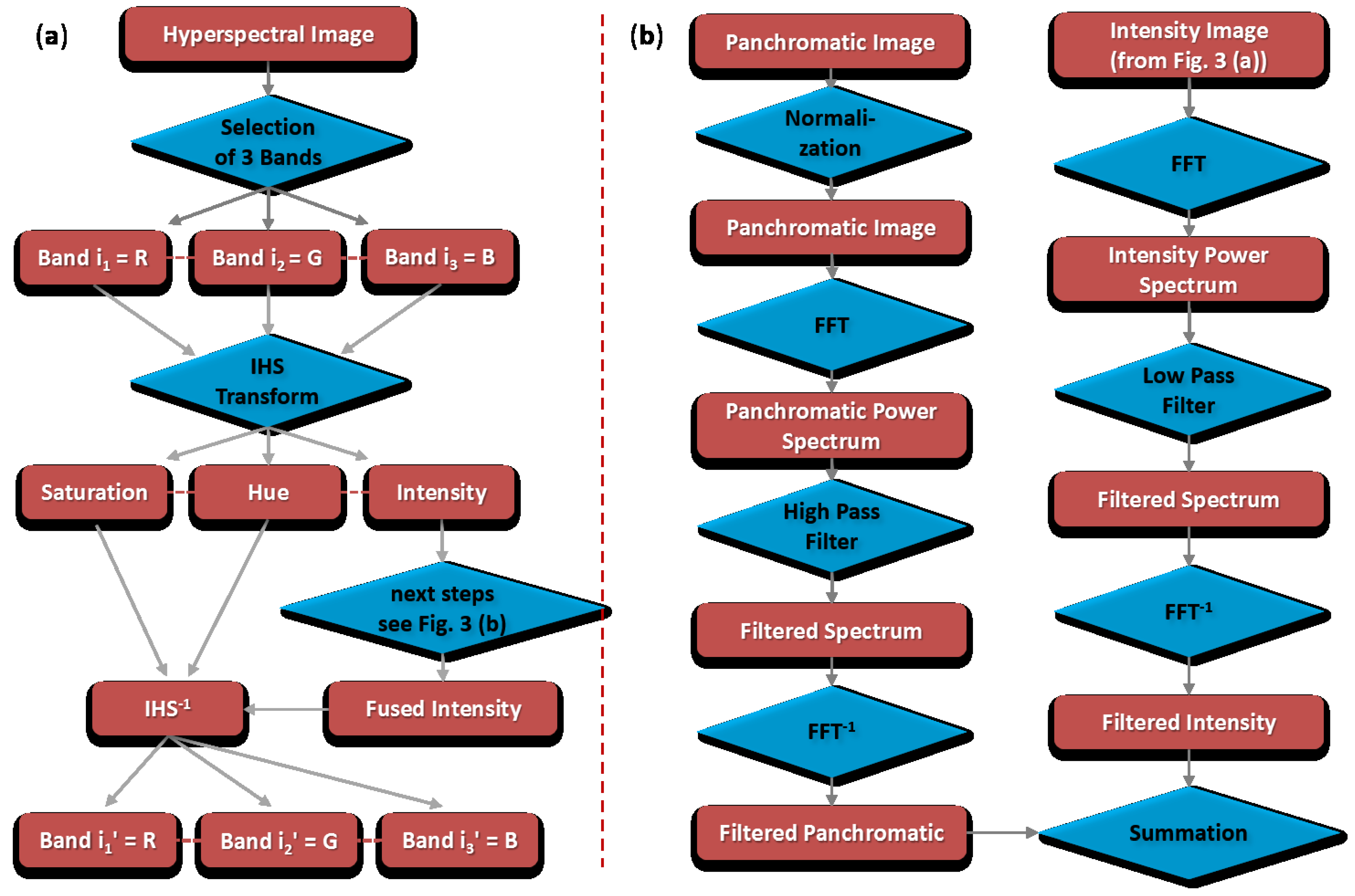
4.1. Ehlers Fusion
- where n = the number of spectral bands
- ti = fused spectrum
- ri = original spectrum
- where n = the number of spectral bands
- ti = fused spectrum
- ri = original spectrum
- µt/r = mean of t or r
4.2. Partial Least Squares Regression
5. Results and Discussion
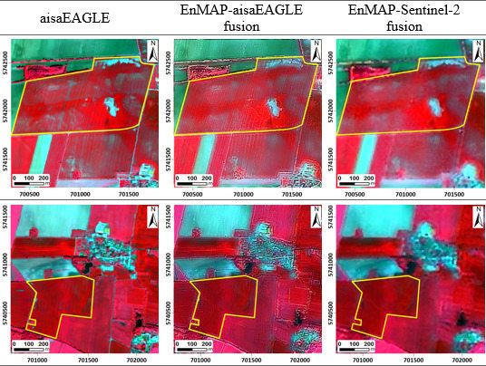
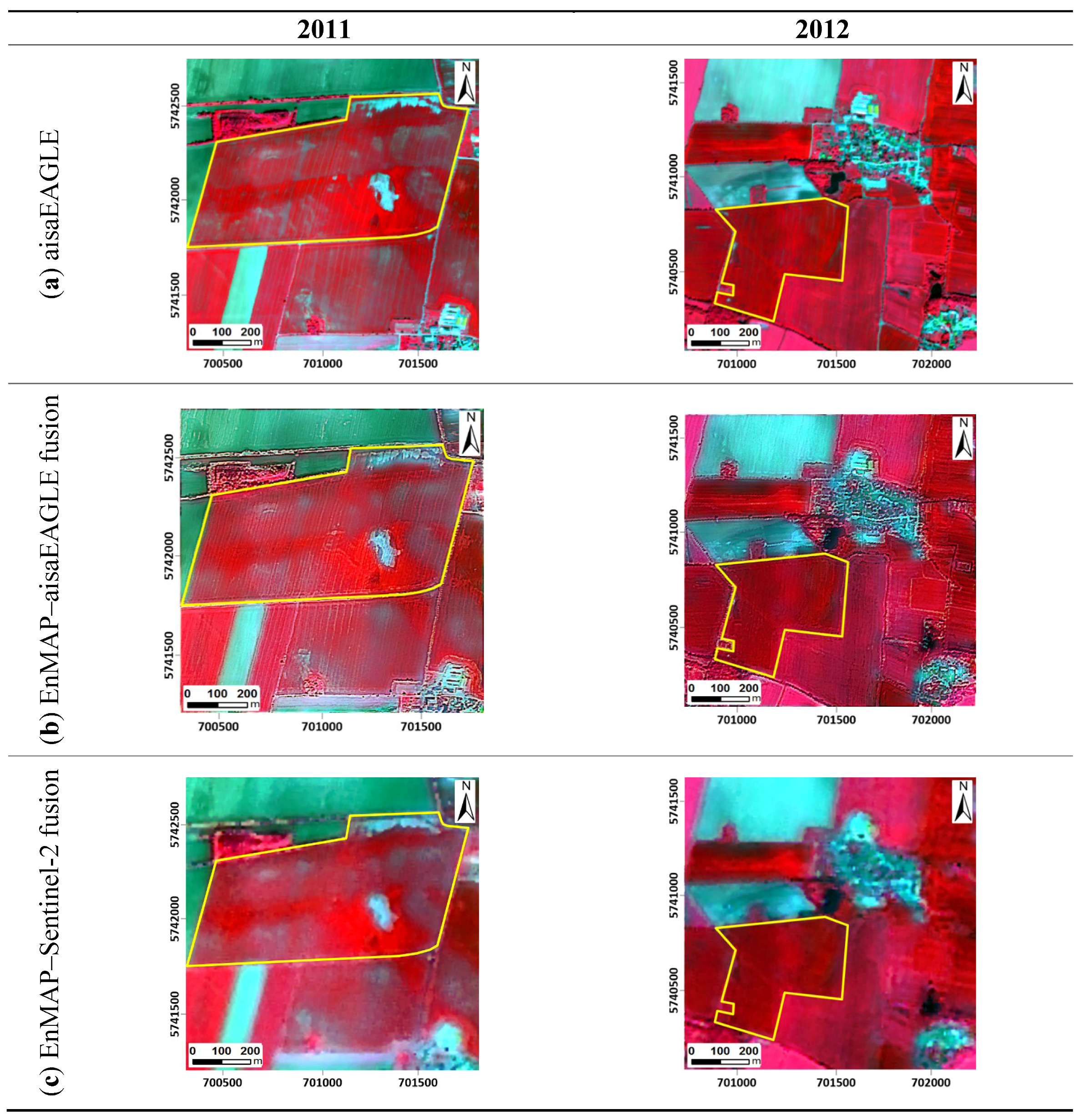
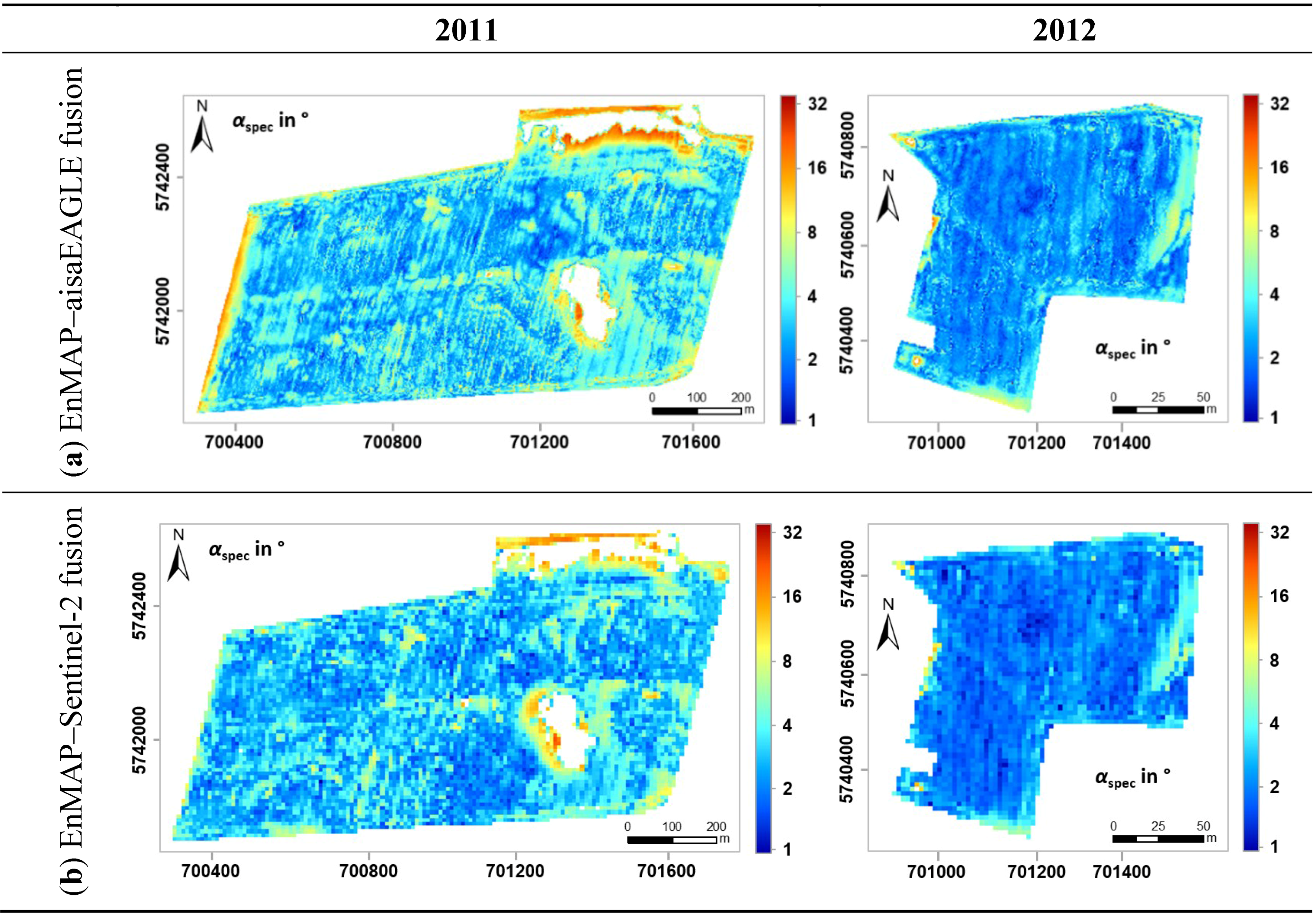
5.1. Image Fusion Results


| Min | Max | Mean | SD | |||||
|---|---|---|---|---|---|---|---|---|
| Year | 2011 | 2012 | 2011 | 2012 | 2011 | 2012 | 2011 | 2012 |
| αspec Image (aisaEAGLE fusion) | 0.56 | 0.60 | 82.49 | 170.46 | 4.51 | 6.74 | 4.34 | 8.79 |
| αspec Field (aisaEAGLE fusion) | 0.56 | 1.01 | 26.57 | 35.17 | 3.02 | 2.65 | 2.49 | 1.28 |
| αspec Image (Sentinel-2 fusion) | 0.55 | 0.53 | 39.61 | 167.32 | 3.63 | 4.51 | 3.54 | 7.94 |
| αspec Field (Sentinel-2 fusion) | 0.58 | 1.06 | 21.82 | 13.34 | 2.50 | 2.33 | 1.84 | 1.02 |
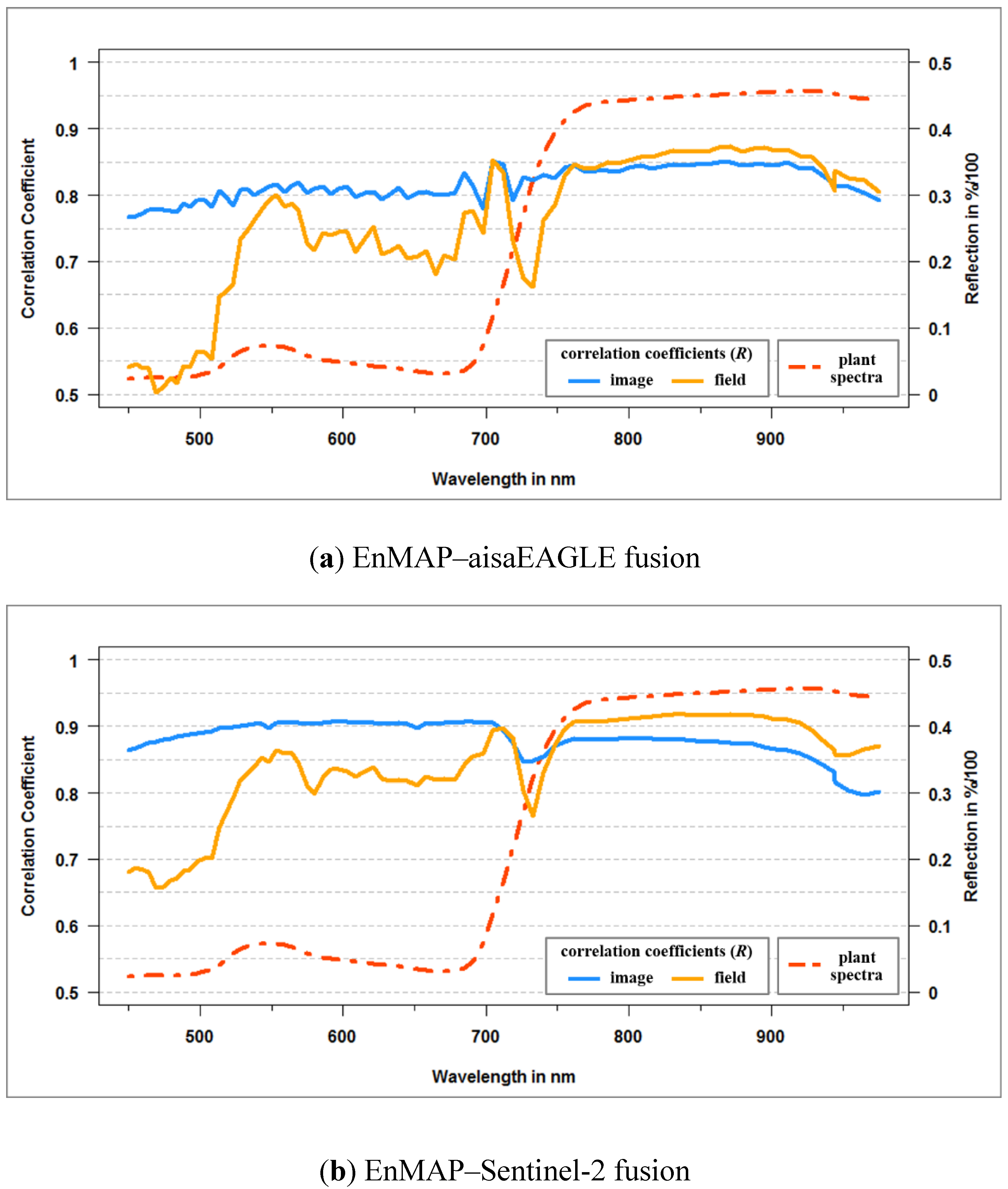
| Correlation Coefficient (R) | Min | Max | Mean | SD | ||||
|---|---|---|---|---|---|---|---|---|
| Image | Field | Image | Field | Image | Field | Image | Field | |
| R EnMAP–aisaEAGLE fusion | 0.77 | 0.50 | 0.85 | 0.87 | 0.82 | 0.75 | 0.02 | 0.11 |
| R Field EnMAP–Sentinel-2 fusion | 0.80 | 0.66 | 0.91 | 0.92 | 0.88 | 0.83 | 0.03 | 0.08 |
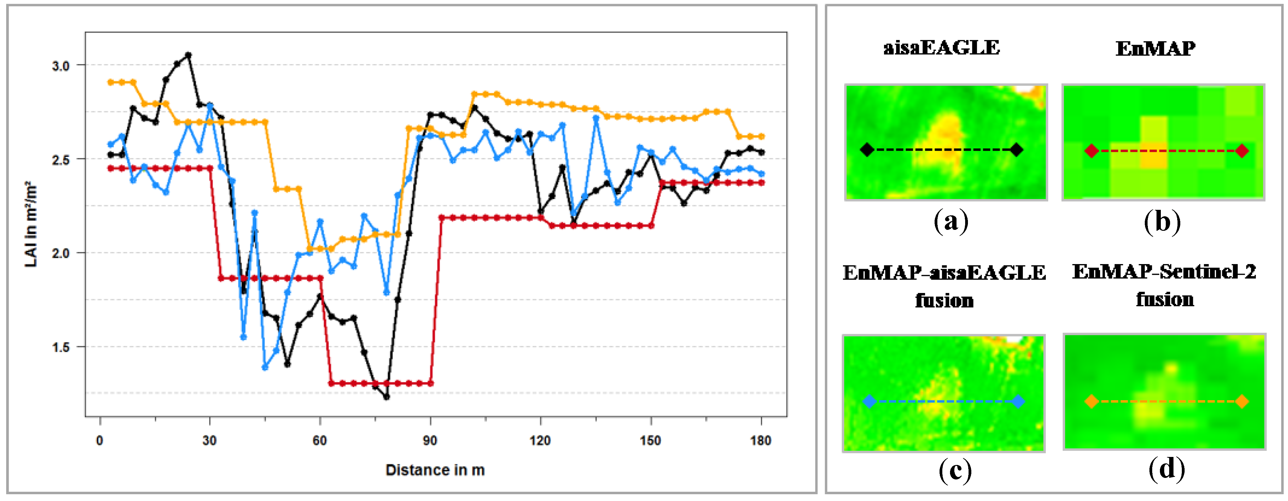
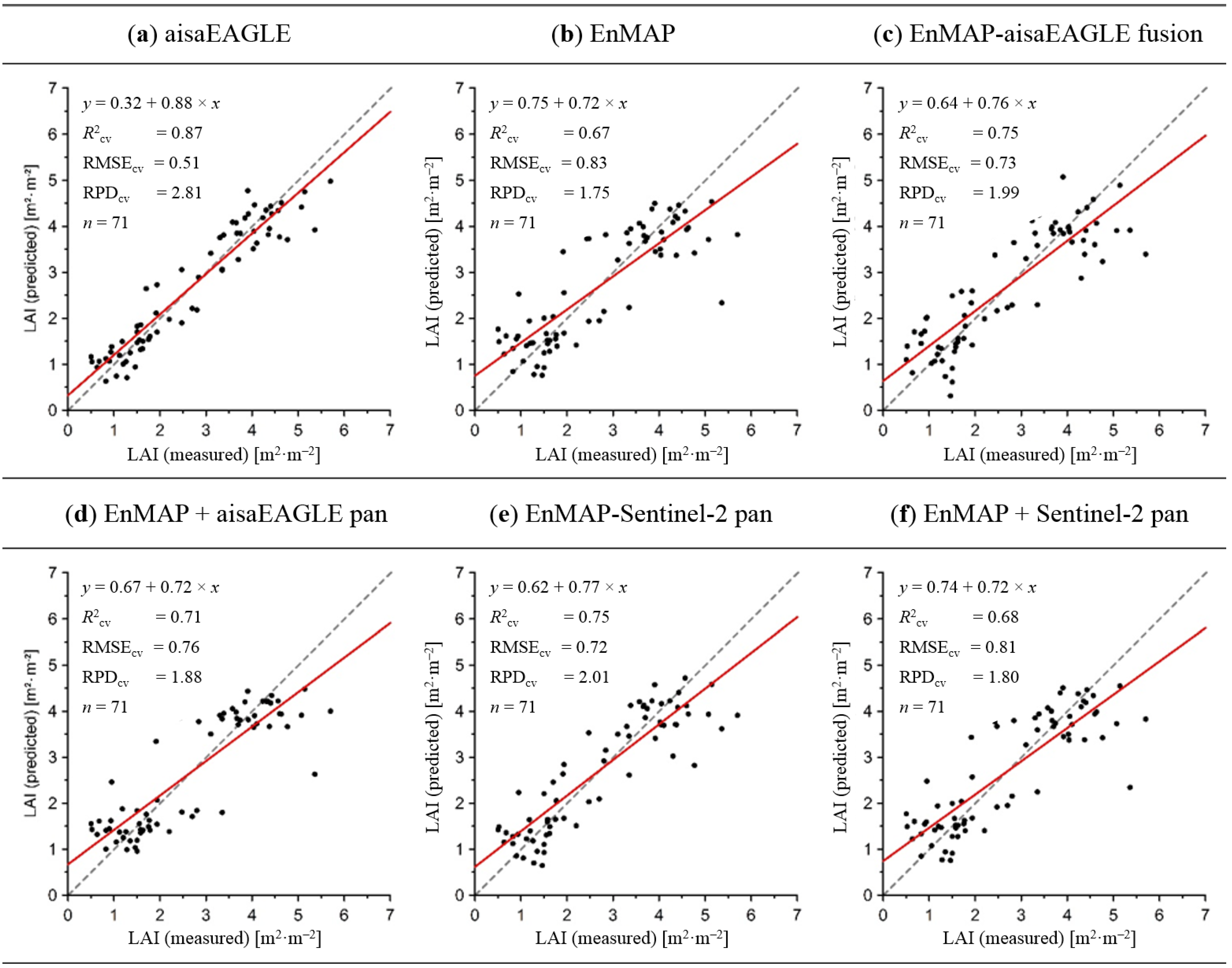
5.2. LAI Retrieval
| n | Min | Max | Mean | SD |
|---|---|---|---|---|
| 36 (2011) | 0.50 | 3.35 | 1.49 | 0.65 |
| 35 (2012) | 1.91 | 5.70 | 3.95 | 0.83 |
| 71 (2011 & 2012) | 0.50 | 5.70 | 2.70 | 1.44 |
| n = 71 | R2cv | RMSEcv | RPDcv |
|---|---|---|---|
| aisaEAGLE | 0.87 | 0.51 | 2.81 |
| EnMAP | 0.67 | 0.83 | 1.75 |
| EnMAP–aisaEAGLE fusion | 0.75 | 0.73 | 1.99 |
| EnMAP + aisaEAGLE pan | 0.71 | 0.76 | 1.88 |
| EnMAP–Sentinel-2 fusion | 0.75 | 0.72 | 2.01 |
| EnMAP + Sentinel-2 pan | 0.68 | 0.81 | 1.80 |


6. Conclusion and Outlook
Acknowledgments
Author Contributions
Conflicts of Interest
References
- Moran, M.S.; Inoue, Y.; Barnes, E.M. Opportunities and limitations for image-based remote sensing in precision crop management. Remote Sens. Environ. 1997, 61, 319–346. [Google Scholar] [CrossRef]
- Gebbers, R.; Adamchuck, V. Precision agriculture and food security. Science 2010, 327, 828–831. [Google Scholar] [CrossRef] [PubMed]
- Seelan, K.S.; Laguetta, S.; Casady, G.M.; Seielstad, G.A. Remote sensing applications for precision agriculture: A learning community approach. Remote Sens. Environ. 2003, 88, 157–169. [Google Scholar] [CrossRef]
- Zhang, N.; Wang, M.; Wang, N. Precision agriculture—A worldwide overview. Comput. Electron. Agric. 2002, 36, 113–132. [Google Scholar] [CrossRef]
- Zarco-Tejada, P.J.; Ustin, S.L.; Whiting, M.L. Temporal and spatial relationships between within-field yield variability in cotton and high-spatial hyperspectral remote sensing imagery. Agron. J. 2005, 97, 641–653. [Google Scholar] [CrossRef]
- Cox, S. Information technology: The global key to precision agriculture and sustainability. Comput. Electron. Agric. 2002, 36, 93–111. [Google Scholar] [CrossRef]
- Mulla, D.J. Twenty five years of remote sensing in precision agriculture: Key advances and remaining knowledge gaps. Biosyst. Eng. 2013, 114, 358–371. [Google Scholar] [CrossRef]
- Schueller, J.K. A review and integrating analysis of spatially-variable control of crop production. Fertil. Res. 1992, 33, 1–34. [Google Scholar] [CrossRef]
- Delécolle, R.; Maas, S.J.; Guérif, M.; Baret, F. Remote sensing and crop production models: Present trends. ISPRS J. Photogramm. Remote Sens. 1992, 47, 145–161. [Google Scholar] [CrossRef]
- Machwitz, M.; Giutarini, L.; Bossung, C.; Frantz, D.; Schlerf, M.; Lilienthal, H.; Wandera, L.; Matgen, P.; Hoffmann, L.; Udelhoven, T. Enhanced biomass prediction by assimilating satellite data into a crop growth model. Environ. Model. Softw. 2014, 62, 437–453. [Google Scholar] [CrossRef]
- Moulin, S.; Bondeau, A.; Delécolle, R. Combining agricultural crop models and satellite observation: From field to regional scales. Int. J. Remote Sens. 1998, 19, 1021–1036. [Google Scholar] [CrossRef]
- Monteith, J.L.; Unsworth, M.H. Principles of Environmental Physics, 4th ed.; Elsevier/Academic Press: London, UK, 2013; p. 418. [Google Scholar]
- Boegh, E.; Soegaard, H.; Broge, N.; Hasager, C.B.; Jensen, N.O.; Schelde, K.; Thomsen, A. Airborne multispectral data for quantifying leaf area index, nitrogen concentration, and photosynthetic efficiency in agriculture. Remote Sens. Environ. 2002, 81, 179–193. [Google Scholar] [CrossRef]
- Carter, G.A. Ratios of leaf reflectances in narrow wavebands as indicators of plant stress. Int. J. Remote Sens. 1994, 15, 697–703. [Google Scholar] [CrossRef]
- Daughtry, C.S.T.; Gallo, K.P.; Goward, S.N.; Prince, S.D.; Kustas, W.D. Spectral estimates of absorbed radiation and phytomass production in corn and soybean canopies. Remote Sens. Environ. 1992, 39, 141–152. [Google Scholar] [CrossRef]
- Dale, L.M.; Thewis, A.; Boudry, C.; Rotar, I.; Dardenne, P.; Baeten, V.; Fernández Pierna, J.A. Hyperspectral imaging applications in agriculture and agro-food product quality and safety control: A review. Appl. Spectrosc. Rev. 2013, 48, 142–159. [Google Scholar] [CrossRef]
- Chen, Z.; Pu, H.; Wang, B. Fusion of hyperspectral and multispectral images: A novel framework based on generalization of pan-sharpening methods. IEEE Geosci. Remote Sens. Lett. 2014, 11, 1418–1422. [Google Scholar] [CrossRef]
- Mayumi, N.; Iwasaki, A. Image sharpening using hyperspectral and multispectral data. IEEE Int. Geosci. Remote Sens. Symp. 2011. [Google Scholar] [CrossRef]
- Johnson, B. Effects of pansharpening on vegetation indices. ISPRS Int. J. Geo-Inf. 2014, 3, 507–522. [Google Scholar] [CrossRef]
- Pinter, P.J., Jr.; Hatfield, J.L.; Schepers, J.S.; Barnes, E.M.; Moran, M.S.; Daughtry, C.S.T.; Upchurch, D.R. Remote Sensing for Crop Management. Photogramm. Eng. Remote Sens. 2003, 69, 647–664. [Google Scholar] [CrossRef]
- Baret, F.; Houlès, V.; Guérif, M. Quantification of plant stress using remote sensing observations and crop models: The case of nitrogen management. J. Exp. Bot. 2007, 58, 869–880. [Google Scholar] [CrossRef] [PubMed]
- Vuolo, F.; Essl, L.; Atzberger, C. Costs and benefits of satellite-based tools for irrigation management. Front. Environ. Sci. 2015, 3, 1–12. [Google Scholar] [CrossRef]
- Ehlers, M.; Klonus, S.; Astrand, P.; Rosso, P. Multi-sensor image fusion for pansharpening in remote sensing. Int. J. Image Data Fusion 2010, 1, 25–45. [Google Scholar] [CrossRef]
- Pohl, C.; van Genderen, J. Structuring contemporary remote sensing image fusion. Int. J. Image Data Fusion 2015, 6, 3–21. [Google Scholar] [CrossRef]
- Zhang, Y. Wavelet-based Bayesian fusion of multispectral and hyperspectral images using Gaussian scale mixture model. Int. J. Image Data Fusion 2012, 3, 23–37. [Google Scholar] [CrossRef]
- Delalieux, S.; Zarco-Tejada, P.J.; Tits, L.; Jiménez Bello, M.Á.; Intrigliolo, D.S.; Somers, B. Unmixing-based fusion of hyperspatial and hyperspectral airborne imagery for early detection of vegetation stress. IEEE Sel. Top. Appl. Earth Obs. Remote Sens. 2014, 7, 2571–2582. [Google Scholar] [CrossRef]
- Zhang, Y.; de Backer, S.; Scheunders, P. Noise-resistant wavelet-based Bayesian fusion of multispectral and hyperspectral images. IEEE Trans. Geosci. Remote Sens. 2009, 47, 3834–3843. [Google Scholar] [CrossRef]
- Chaudhuri, S.; Kotwal, K. Hyperspectral Image Fusion, 1st ed.; Springer: New York, NY, USA, 2013; p. 191. [Google Scholar]
- Zurita-Milla, R.; Clevers, J.G.P.W.; Shaepman, M.E. Unmixing-based Landsat TM and MERIS FR data fusion. IEEE Geosci. Remote Sens. Lett. 2008, 5, 453–457. [Google Scholar] [CrossRef]
- Amorós-López, J.; Gómez-Chova, L.; Alonso, L.; Guanter, L.; Zurita-Milla, R.; Moreno, M.; Camps-Valls, G. Multitemporal fusion of Landsat/TM and ENVISAT/MERIS for crop monitoring. Int. J. Appl. Earth Obs. Geoinformation 2013, 23, 132–141. [Google Scholar] [CrossRef]
- Gevaert, C.M.; Tang, J.; García-Haro, F.J.; Suomalainen, J.; Kooistra, L. Combining hyperspectral UAV and multispectral Formosat-2 imagery for precision agriculture applications. In Proceedings 6th Workshop on Hyperspectral Image and Signal Processing: Evolution in Remote Sensing (WHISPERS), Lausanne, Switzerland, 24–27 June 2014.
- Klonus, S.; Ehlers, M. Image fusion using the Ehlers spectral characteristics preserving algorithm. GIScience Remote Sens. 2007, 44, 93–116. [Google Scholar] [CrossRef]
- Ling, Y.; Ehlers, M.; Usery, E.L.; Madden, M. FFT-enhanced IHS transform method for fusing high-resolution satellite images. ISPRS J. Photogramm. Remote Sens. 2007, 61, 381–392. [Google Scholar] [CrossRef]
- Jawak, S.D.; Luis, A.J. A comprehensive evaluation of PAN-sharpening algorithms coupled with resampling methods for image synthesis of very high resolution remotely sensed satellite data. Adv. Remote Sens. 2013, 2, 332–344. [Google Scholar] [CrossRef]
- Rogaß, C.; Spengler, D.; Bochow, M.; Segl, K.; Lausch, A.; Doktor, D.; Roessner, S.; Behling, R.; Wetzel, H.U.; Kaufmann, H. Reduction of radiometric miscalibration-application to pushbroom sensors. Sensors 2011, 11, 6370–6395. [Google Scholar] [CrossRef] [PubMed]
- Berk, A.; Bernstein, L.S.; Anderson, G.P.; Acharya, P.K.; Robertson, D.C.; Chetwynd, J.H.; Adler-Golden, S.M. MODTRAN cloud and multiple scattering upgrades with application to AVIRIS. Remote Sens. Environ. 1998, 65, 367–375. [Google Scholar] [CrossRef]
- Smith, G.M.; Milton, E.J. The use of the empirical line method to calibrate remotely sensed data to reflectance. Int. J. Remote Sens. 1999, 20, 2653–2662. [Google Scholar] [CrossRef]
- Segl, K.; Guanter, L.; Rogass, C.; Kuester, T.; Roessner, S.; Kaufmann, H.; Sang, B.; Mogulsky, V.; Hofer, S. EeteS—The EnMAP end-to-end simulation tool. IEEE J. Sel. Top. Appl. Earth Obs. Remote Sens. 2012, 5, 522–530. [Google Scholar] [CrossRef]
- Segl, K.; Guanter, L.; Kaufmann, H. Simulation of spatial sensor characteristics in the context of the EnMAP hyperspectral mission. IEEE Trans. Geosci. Remote Sens. 2010, 48, 3046–3054. [Google Scholar] [CrossRef]
- Guanter, L.; Segl, K.; Kaufmann, H. Simulation of optical remote sensing scenes with application to the EnMAP hyperspectral mission. IEEE Trans. Geosci. Remote Sens. 2009, 47, 2340–2351. [Google Scholar] [CrossRef]
- Sentinel Online. Available online: https://sentinel.esa.int/web/sentinel/user-guides/sentinel-2-msi/resolutions/radio-metric (accessed on 7 May 2015).
- Kruse, F.A.; Lefkoff, A.B.; Boardman, J.W.; Heidebrecht, K.B.; Shapiro, A.T.; Barloon, P.J. The spectral image processing system (SIPS)—Interactive visualization and analysis of imaging spectrometer data. Remote Sens. Environ. 1993, 44, 145–163. [Google Scholar] [CrossRef]
- Alparone, L.; Wald, L.; Chanussot, J.; Thomas, C.; Gamba, P.; Bruce, L.M. Comparison of pansharpening algorithms: Outcome of the 2006 GRS-S Data-Fusion Contest. IEEE Trans. Geosci. Remote Sens. 2007, 45, 3012–3021. [Google Scholar] [CrossRef]
- Darvishzadeh, R.; Skidmore, A.; Schlerf, M.; Atzberger, C.; Corsi, F.; Cho, M. LAI and chlorophyll estimation for a heterogeneous grassland using hyperspectral measurements. ISPRS J. Photogramm. Remote Sens. 2008, 63, 409–426. [Google Scholar] [CrossRef]
- Jarmer, T. Spectroscopy and hyperspectral imagery for monitoring summer barley. Int. J. Remote Sens. 2013, 34, 6067–6078. [Google Scholar] [CrossRef]
- Pu, R. Comparing canonical correlation analysis with partial least squares regression in estimating forest leaf area index with multitemporal landsat TM imagery. GIScience Remote Sens. 2013, 49, 92–116. [Google Scholar] [CrossRef]
- Siegmann, B.; Jarmer, T. Comparison of different regression models and validation techniques for the assessment of wheat leaf area index from hyperspectral data. Int. J. Remote Sens. 2015, in press. [Google Scholar]
- Rännar, S.; Geladi, P.; Lidgren, F.; Wold, S. A PLS kernel algorithm for data sets with many variables and fewer objects. Part 1: Theory and algorithm. J. Chemom. 1994, 8, 111–124. [Google Scholar] [CrossRef]
- Akaike, H. A new look at the statistical model identification. IEEE Trans. Autom. Control 1974, 19, 716–723. [Google Scholar] [CrossRef]
- Malley, D.F.; Martin, P.D.; Ben-Dor, E. Application in analysis of soils. In Near-Infrared Spectroscopy in Agriculture, 1st ed.; Roberts, C.A., Workman, J., Jr., Reeves, J.B., III, Eds.; American Society of Agronomy; Crop Science Society of America; Soil Science Society of America: Madison, WI, USA, 2004; pp. 729–783. [Google Scholar]
- Williams, P.C. Implementation of near-infrared technology. In Near-Infrared Technology in the Agricultural and Food Industries, 2nd ed.; Williams, P., Norris, K., Eds.; American Association of Cereal Chemists: St. Paul, MN, USA, 2001; pp. 145–169. [Google Scholar]
- Dunn, B.W.; Beecher, H.G.; Batten, G.D.; Ciavarella, S. The potential of near-infrared reflectance spectroscopy for soil analysis: A case study from the Riverine plain of South-Eastern Australia. Aust. J. Exp. Agric. 2002, 42, 607–614. [Google Scholar] [CrossRef]
- Otto, M. Chemometrics: Statistics and Computer Application in Analytical Chemistry, 2nd ed.; Wiley-VCH: New York, NY, USA, 2007; p. 343. [Google Scholar]
- Rollin, M.E.; Milton, E.J. Processing of high spectral resolution reflectance data for the retrieval of canopy water content information. Remote Sens. Environ. 1998, 65, 86–92. [Google Scholar] [CrossRef]
- Ehlers, M. Rectification and registration. In Integration of Remote Sensing and GIS, 1st ed.; Star, J.L., Estes, J.E., McGwire, K.C., Eds.; Cambridge University Press: Cambridge UK, 1997; pp. 13–36. [Google Scholar]
- Ehlers, M.; Jacobsen, K.; Schiewe, J. High Resolution Image Data and GIS. In ASPRS Manual of GIS, 1st ed.; Madden, M., Ed.; American Society for Photogrammetry and Remote Sensing: Bethesda, MD, USA, 2009; pp. 721–777. [Google Scholar]
- Landsat Science. Available online: http://landsat.gsfc.nasa.gov/?p=5771 (accessed on 7 May 2015).
- SPOT 6 SPOT 7 Technical Sheet. Available online: http://www2.geo-airbusds.com/files/pmedia/public/r12317_9_spot6–7_technical_sheet.pdf (accessed on 7 May 2015).
- Chander, G.; Markham, B.L.; Helder, D.L. Summary of current radiometric calibration coefficients for Landsat MSS, TM, ETM+, and EO-1 ALI sensors. Remote Sens. Environ. 2009, 113, 893–903. [Google Scholar] [CrossRef]
- Black Bridge Imagery Products. Available online: http://www.blackbridge.com/geomatics/products/rapideye.html (accessed on 13 May 2015).
- Padwick, C.; Deskevich, M.; Pacifici, F.; Smallwood, S. WorldView-2 pan-sharpening. In Proceedings of the 2010 ASPRS Annual Conference, San Diego, CA, USA, 26–30 June 2010.
© 2015 by the authors; licensee MDPI, Basel, Switzerland. This article is an open access article distributed under the terms and conditions of the Creative Commons Attribution license (http://creativecommons.org/licenses/by/4.0/).
Share and Cite
Siegmann, B.; Jarmer, T.; Beyer, F.; Ehlers, M. The Potential of Pan-Sharpened EnMAP Data for the Assessment of Wheat LAI. Remote Sens. 2015, 7, 12737-12762. https://doi.org/10.3390/rs71012737
Siegmann B, Jarmer T, Beyer F, Ehlers M. The Potential of Pan-Sharpened EnMAP Data for the Assessment of Wheat LAI. Remote Sensing. 2015; 7(10):12737-12762. https://doi.org/10.3390/rs71012737
Chicago/Turabian StyleSiegmann, Bastian, Thomas Jarmer, Florian Beyer, and Manfred Ehlers. 2015. "The Potential of Pan-Sharpened EnMAP Data for the Assessment of Wheat LAI" Remote Sensing 7, no. 10: 12737-12762. https://doi.org/10.3390/rs71012737
APA StyleSiegmann, B., Jarmer, T., Beyer, F., & Ehlers, M. (2015). The Potential of Pan-Sharpened EnMAP Data for the Assessment of Wheat LAI. Remote Sensing, 7(10), 12737-12762. https://doi.org/10.3390/rs71012737