Graph-Based Divide and Conquer Method for Parallelizing Spatial Operations on Vector Data

Abstract
: In computer science, dependence analysis determines whether or not it is safe to parallelize statements in programs. In dealing with the data-intensive and computationally intensive spatial operations in processing massive volumes of geometric features, this dependence can be well utilized for exploiting the parallelism. In this paper, we propose a graph-based divide and conquer method for parallelizing spatial operations (GDCMPSO) on vector data. It can represent spatial data dependences in spatial operations through representing the vector features as graph vertices, and their computational dependences as graph edges. By this way, spatial operations can be parallelized in three steps: partitioning the graph into graph components with inter-component edges firstly, simultaneously processing multiple subtasks indicated by the graph components secondly and finally handling remainder tasks denoted by the inter-component edges. To demonstrate how it works, buffer operation and intersection operation under this paradigm are conducted. In a 12-core environment, the two spatial operations both gain obvious performance improvements, and the speedups are more than eight. The testing results suggest that GDCMPSO contributes to a method for parallelizing spatial operations and can greatly improve the computing efficiency on multi-core architectures.1. Introduction
Spatial operations refer to the use of geometry functions to take spatial data as input, analyze the data, and then produce output data that is the derivative of the analysis performed on the input data [1]. From the perspectives of mathematics and computer science, the input is, or are, termed spatial operand, or operands, and the method to analyze the data is termed spatial operator. In practice, different applications use different operators, and a common distinction between different categories of spatial operators is based on the different geometric properties of spatial relations, leading to groups of topological, directional, and metric relations [2]. Currently, various spatial operators have been realized in current commercial GIS (Geographic Information Science) Systems [3]. The main operators defined by the “Open Geospatial Consortium, Inc.” (OGC) are implemented by a set of geometry operations on geometry values in ArcGIS software, and they include the intersection of geometries, difference of geometries, union of geometries, symmetric difference of geometries, buffering zone of geometries, and convex hull of geometries [4], and a common characteristic is that all these operators create new data from input data [1].
The spatial operations have been widely used in many fields, including site selection [5,6], spatial decision making [7,8], crisis and disaster management [8,9], etc. Another significant application of spatial operations is geographical conditions monitoring (GeoCM), which currently has become a research focus in China and other countries [10]. GeoCM can be divided into fundamental monitoring, thematic monitoring, and disaster monitoring [11]. Among these aspects, fundamental monitoring mainly focuses on monitoring all of the geographical elements in a national scale, and kinds of spatial operations are increasingly being used in searching and processing of massive spatial geometries. Along with the fact that the location-aware datasets, professional data or volunteered geographic information (VGI), are of a size, variety, and update rate that exceeds the capability of spatial computing technologies [12], there is an urgent demand to improve the processing performance of these operations in the change monitoring field. In these processes, the spatial features act as the primary medium of representing the geographic information, as evidenced by their geometric shapes and their spatial relations. A feature is anything that can be seen on the landscape, such as houses, roads, rivers and land parcels. The spatial relations involve topological relations, metric relations, and relations about the order of the spatial objects [13,14]. In the reconstruction of 3D building models, the topological relations between the building parts could be represented by the topology graph [15]. In addition, the spatial relations can be understood from a empirical perspective, as in the observation known as Tobler’s first law of geography [16], or from a theoretical perspective, as in the fundamental contribution known as the Nine-intersection of topology [17].
In this paper, we are particularly concentrated on how to improve the performance of spatial operations in processing massive vector features. Herein, we use a graph-based method to represent the spatial data dependence in spatial operations and then exploit the inherent parallelism by divide and conquer method which has been used in the parallelization of triangulation [18]. Conceptually, this novel method is termed graph-based divide and conquer method for parallelizing spatial operations (GDCMPSO) on vector data, which use the spatial data dependence graph (SDDG) to quantitatively represent the data dependence in spatial operations. The novel method includes two main layers: a representative graph towards the spatial operation (the upper layers) and the computing resources (the bottom layer). The representative graph is used for the spatial decomposition, and it enables partitioning a spatial operation into multiple subtasks with balanced working loads and recording the decomposing positions to guide the combination of the sub-results. Most importantly, with the two functions, the final result can maintain the correctness and consistency, i.e., the final result from a spatial operation under this method is consistent with the result from the sequential algorithm. With the above graph, the power of the computing resources can be exploited easily through simultaneously executing multiple subtasks by multi-core CPUs or computer clusters. In this paper, thread-level parallel computing technologies are well utilized for testing the method. Specifically, a target spatial operator should be firstly represented by the SDDG, and then the parallelism could be obtained by dividing the graph into multiple graph components and simultaneously executing multiple subtasks denoted by these components. Finally, the tasks denoted by the inter-component edges are handled, and this process may be performed iteratively. In this process, two kernel functions should be realized: the vertex function and the edge function, which take charge of processing spatial features, and the relations between features and results from subtasks.
The remainder of the paper is organized as follows. The Section 2 lists the related work and the existed problems. Our proposed method is elucidated in Section 3. In addition, two demonstrating spatial operations are realized and tested in Sections 4 and 5, respectively. Finally in Section 6, we conclude the main contributions and also discuss the future research work.
2. Background and Related Work
2.1. Multi-Core Computing
In recent years, the multi-core processor has been widely used for the enhanced performance, reduced power consumption, and more efficient simultaneous processing of multiple tasks. It adopts scalable shared-memory multiprocessor architectures [19], and each processor can independently read and execute program instructions. Multi-threading has become one of the most common foundations upon which developers build parallel software to leverage the power of a multi-core processor. However, direct threading is difficult and somewhat error-prone [20]. Fortunately, some high-level threading libraries, such as OpenMP (Open Multi-Processing) [21] and TBB (Threading Building Block) [22], offer powerful new ways to achieve high performance in multi-core architectures. OpenMP is an API that supports multi-platform shared-memory multiprocessing programming in C, C++, and Fortran on most processor architectures and operating systems. It uses a portable, scalable model that gives programmers a simple and flexible interface for developing parallel applications for platforms ranging from the standard desktop computer to the supercomputer. TBB is a template library for C++ developed by Intel to parallelize programs. It is available in an open source version, as well as in a commercial version that provides further support. In special classes, parallel code is encapsulated and invoked from the program. As a result, development using these libraries is easier and more convenient because the low level complexities are hidden.
2.2. Computationally Intensive Geocomputation
As a matter of fact, the High Performance Computing (HPC) systems or supercomputers are becoming increasingly devoted to geocomputation, which can be regarded as the application of a large-scale computationally intensive approach to the problems of physical and human geography in particular, and the geosciences in general [23–25]. In addition, it may be helpful to think of geocomputation as a computationally intensive, application-led common of GIScience [17]. The use of HPC technologies in geocomputation can be concluded in two aspects: GIS algorithms and generic solutions.
Firstly, the HPC technologies have been used to improve the performance of a large variety of algorithms in geocomputation. Typical efforts can be demonstrated in spatial interpolation [26–28], spatial statistics [26,29–31], spatial visualization [32], viewshed analysis [33,34], spatial simulation [35,36], geocollaboration [27,37], etc. In most cases, the optimization strategy used in one algorithm may not work for another.
Secondly, some significant efforts have been devoted to the design and development of the fundamental solutions based on the HPC platforms. These fundamental solutions can be the theoretical approaches, such as the grid-based representation of a spatial computational domain [27,30,38], the framework for multilayered libraries between the computing resources and the serial geographic algorithms [39], and the research on the distributed geographic information processing (DGIP) which provides a guiding methodology and principles for implementing geospatial middleware [40–42], or the general libraries for processing a particular category of applications, such as the pRPL (parallel raster processing programming library) [43], the PaRGO (parallel raster-based geocomputation operators) [44], etc. In summary, the implementations of these fundamental solutions are mostly based on the powerful computing technologies, including grid computing, cloud computing, and parallel computing. In other words, the integration of the Cyber-Infrastructure (CI) with the GIS, i.e., Cyber-GIS, may better summarize these solutions.
2.3. Research Problems in Parallelizing Spatial Operations
Great contributions have been made in parallel geographic algorithms and the general-purpose solutions (see Section 2.2). However, three problems still exist.
- (1)
The first problem is the lack of a systematic research on how to exploit the parallelism for vector-based spatial operations. Considerable work has been undertaken to design parallel algorithms for processing raster data, while fewer examples are found involving vector data [39]. The examples from the existing approaches are primarily based on the raster data and the spatial point set. As a matter of fact, the local dependences of these algorithms from these two types of data have enabled a better inherent parallelism. In contrast, complex geometries with irregular shapes and non-uniform computing intensity, such as the linear features and the polygonal features in spatial operations, become difficult to be represented in the existing technological framework. Dividing the study area into a regular grid is a better strategy in processing raster data, but not a general method for processing the vector data. A conceptual and contributed method for boosting the performance of vector data processing is worthy of in-depth study.
- (2)
The second problem is the poor reusability of the existing software or packages. Most of the existing GIS packages, whether commercial or open source, are realized in a sequential mode. The significant costs of parallel re-implementation of the existed algorithm packages impede the full utilization of the parallel technologies [39]. Obviously, re-writing all the modules is inefficient and unfeasible. Therefore, reusability is a basic requirement that should be considered in designing a conceptual method.
- (3)
The third problem is the lack of consideration about the output consistency. In computer science, output dependence (see Section 3.1) can’t be avoided when outputting the related partial results by parallel threads. In fact, most spatial operations create new data from input data. In other words, research is required on methods to distribute, synchronize, integrate, and balance the processing within a distributed environment [42].
The proposed method seeks to resolve the above three problems both in theory and practice. With the graph-based divide and conquer method, a spatial operation on the vector data is represented in SDDG, then the study on how to parallelize the spatial operation is transformed into the graph partitioning problem [45] and the utilization of the thread-level computing technology [21]. As a result, boosting the performance of an existing algorithm only demands the developer to represent the algorithm with the SDDG and write the codes of merging the sub-results. Thus, both the reusability and the consistency can be guaranteed.
3. Methodology
The graph-based divide and conquer method for spatial operations on vector data involves the following main aspects: definition and representation of the spatial data dependence (see Section 3.1 and Section 3.2), partitioning (see Section 3.3) and merging of the spatial data dependence graph (see Section 3.4), and the thread-level parallel engine for scheduling the kernel functions and the computing resources (see Section 3.5). Finally, the complexity of the method is analyzed in Section 3.6.
3.1. The Data Dependence and Parallelism in Spatial Operations
In computer science, an instruction j is data dependent on instruction i if either of the following holds [46]: (i) instruction i produces a result that may be used by instruction j; or (ii) instruction j is data dependent on instruction k and instruction k is data dependent on instruction i. According to Bernstein condition [47], data dependence can be summarized as follows:
Parallelism can be exploited in two levels, instruction-level parallelism (ILP) and thread-level parallelism (TLP). As suggested by Hennessy [46], ILP is reaching its limits due to its inefficiency in energy consumption when increasing performance, and the use of TLP provides an alternative or addition to instruction-level parallelism. To exploit the thread-level parallelism, the thread-level data dependence should be detected and resolved [52]. In other words, to write correct and efficient shared memory programs, programmers need a precise notion of how memory behaves with respect to read and write operations from multiple processors [53]. Specifically, the sequential consistency model for shared memory multiprocessor is commonly introduced, and a multiprocessor system is sequentially consistent if “the result of any execution is the same as if the operations of all the processors were executed in some sequential order, and the operations of each individual processor appear in this sequence in the order specified by its program” [54]. The guidelines in the computer community should also be adopted in parallelizing the spatial operations. Cartographic modeling and forms of mathematical modeling are two basic elements of spatial analysis [55]. The former element indicates that map-based operations usually generate new maps (such as the buffer operation), the latter element indicates that the computing results are dependent on the form of spatial relations between objects. Specifically, the generated results from spatial operations are constrained to the spatial relations inherently in spatial data. For one example, the distance measurement is often used in generating the buffer zones to determine whether or not the dissolving option is required to union the generated zones. For another example, topological analysis is used in overlaying two vector layers to determine whether a pair of objects is intersected. In these processes, the output data dependence may occur when processing of different features writes the same result. The measurement of the spatial data dependence can filter out the unnecessary computing loads, and this is the first step for exploiting the parallelism.
3.2. Graph-Based Representation of the Data Dependence for Spatial Operations
In spatial operations, spatial operators over more than two operands are typically broken down into a sequence of binary operations [2]. Herein, the binary relation between any pair of the features can be categorized into two types, dependent relationship and independent relationship.
Definition 1: dependent relation ↔.
Given a pair of features Fi and Fj, represented by graph vertices i and j, then Fi ↔ Fj, iff: i ≠ j and the output of the computation based on feature Fi contradicts with the output of the computation based on Fj.
Definition 2: independent relation ‖.
Given a pair of features Fi and Fj, represented by graph vertices i and j, then Fi ‖ Fj, iff: i ≠ j and the output of the computation based on feature Fi and the output of the computation based on feature Fj, are mutually independently.
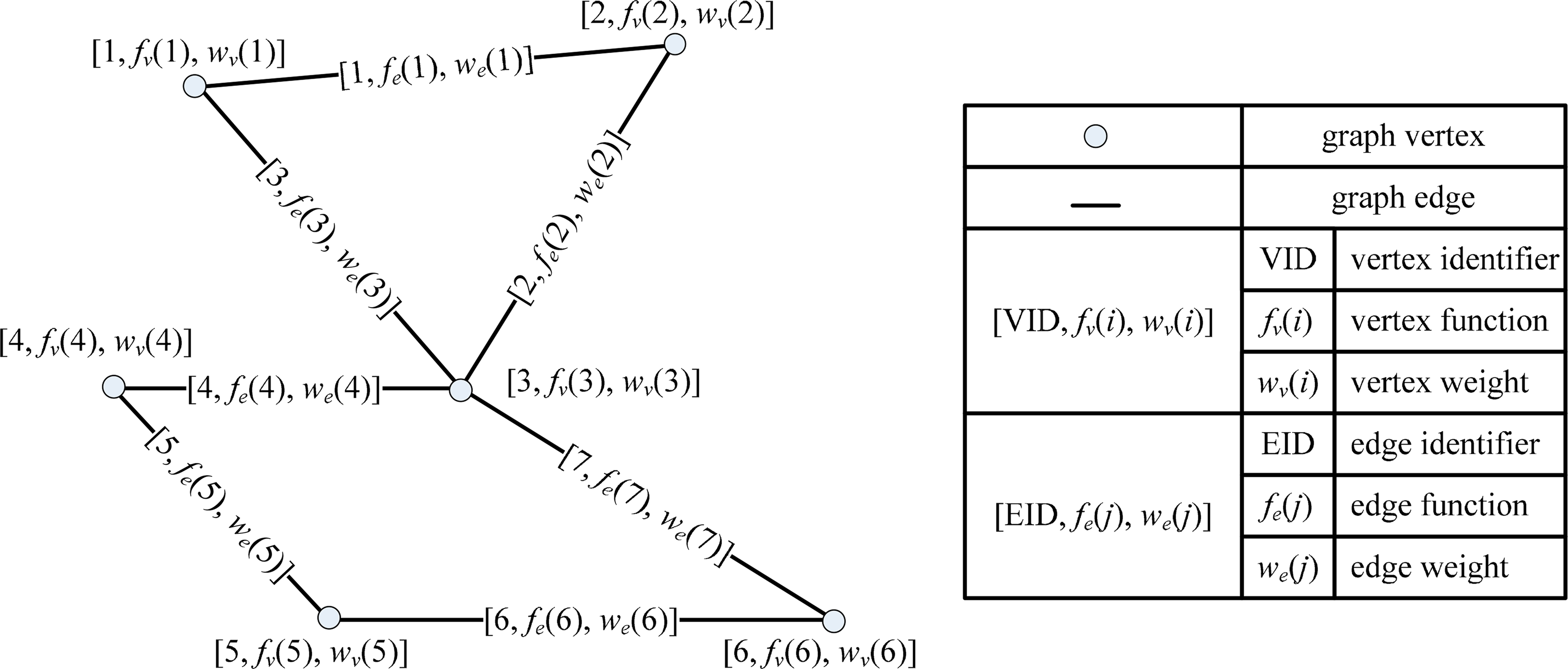
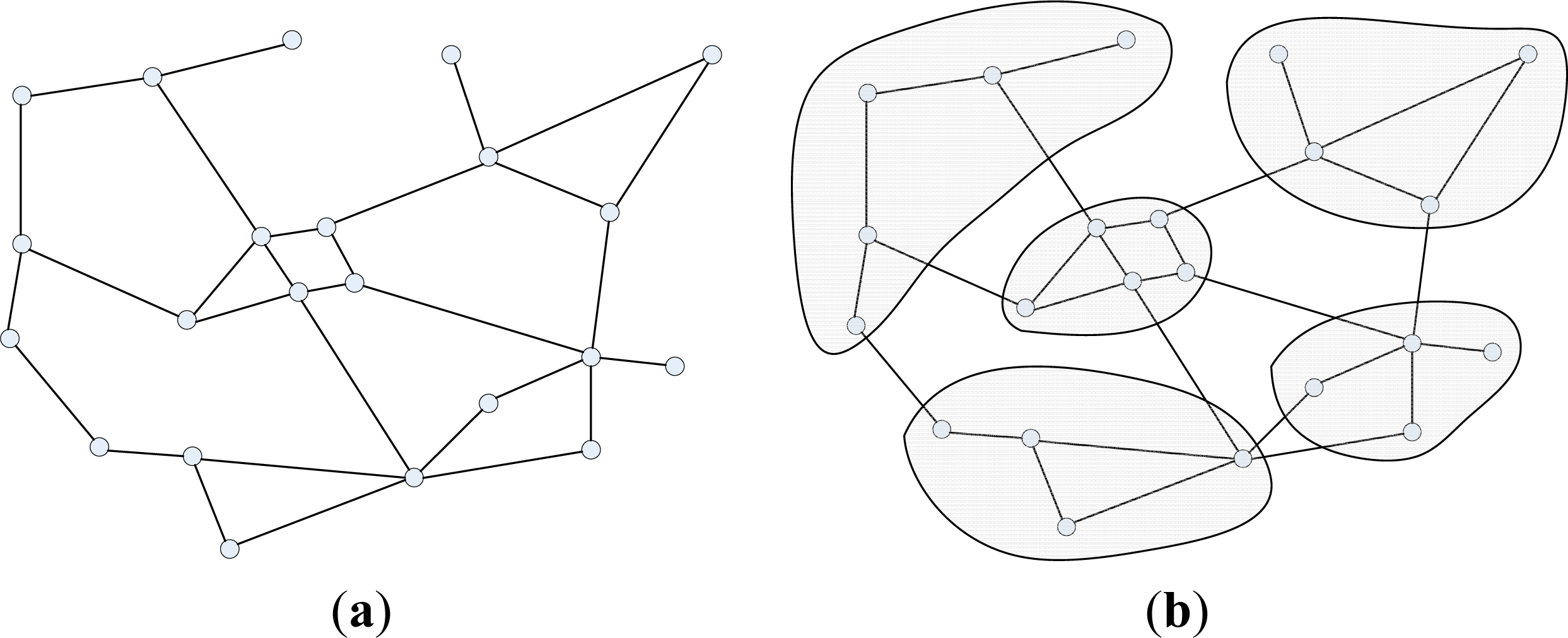
With the above relations, a spatial operation can be represented as the SDDG: the processing of each feature is represented as a vertex and the processing of each dependent relation is represented as an edge (see Figure 1). A SDDG can be formally modeled by the following Formula:
When building a SDDG, the weight for each vertex and the weight for each dependent edge should be firstly determined. Generally, the weight for each vertex depends on both the data and vertex function, and the weight for each edge depends on both the dependent relation and the edge function. Herein, the vertex function and the edge function are closely related with the spatial operations. GIS software libraries provide functionality that can be used by other applications [56], and these libraries, whether commercial or open source, have provided APIs that enable access to a wide range of analysis functions. Therefore, both of the two functions can be easily realized by encapsulating the existing modules, such that the reusability of existing GIS functions for spatial operations is feasible.
3.3. Partitioning of the SDDG Using Divide and Conquer Method
After building the SDDG, the next step is to partition this graph. In mathematics, the graph partitioning problem is defined on data represented in the form of a graph G = (V, E), with V vertices and E edges, such that it is possible to partition G into smaller components with specific properties [57]. Graph partitioning arises as a preprocessing step to divide and conquer algorithms, where it is often a good idea to break things into roughly equal-sized pieces [58]. Partitioning a graph into equal sized components while minimizing the number of edges between different components can contribute to a balanced task assigning strategy in parallel computing [45,59]. By this way, the computing load can be divided among processors of a parallel computer [60]. Herein, if the SDDG can be partitioned into multiple approximately equal components, a spatial operation can be partitioned into multiple subtasks with equally sized computational intensities.
Many algorithms have been developed to find a reasonably good partition. Typical methods include spectral portioning methods [61], geometric partition algorithms [62–64], and the multilevel graph partitioning algorithms [65–68]. The multilevel graph partitioning algorithms work by applying one or more stages. Each stage reduce the size of the graph by collapsing vertices and edges, partition the smaller graph, then maps back and refines this partition of the original graph [68]. In many cases, this approach can give both fast execution times and very high quality results. One widely used example of such an approach is called METIS [45], which was developed in the Karypis lab [69]. METIS provides a set of programs for partitioning graphs, partitioning finite element meshes, and producing fill-reducing orderings for sparse matrices. The algorithms implemented in METIS are based on the multilevel recursive-bisection, multilevel k-way, and multi-constraint partitioning schemes. Herein, the multilevel k-way partitioning scheme is selected as the partitioner in the proposed method. This is because METIS’s multilevel k-way partitioning algorithm provides the advantageous capabilities of the minimized resulting sub-domain connectivity graph, enforced contiguous partitions and minimized alternative objectives. One of the objectives of the k-way partitioning algorithm in METIS is to minimize the number of the edges that are straddled [70]. Figure 2 shows the principle of partitioning a sample SDDG. Figure 2a is a sample SDDG, the corresponding partitioning components are displayed in Figure 2b. For a spatial operation, partitioning the SDDG in this way can contribute two advances for exploiting the parallelism: balanced computing loads among different tasks and the minimum cost of merging the results from these tasks. The first advance is the key for parallelizing the spatial operations. With this decomposing strategy, the minimum cost of dividing the spatial data is achieved. In comparison with the regular data decomposition in processing raster data, the cost of dividing the irregular and complex geometries can be avoided.
3.4. Merging of the Linkages between SDDG Components
In conjunction with the partitioning of the SDDG is the handling of the linkages between the SDDG components. In essence, the linkages between the SDDG components are also the linkages between features. Therefore, edge function is applied equally to the linkages between SDDG the components. Herein, the handling of the linkages is determined by the data dependence, and two situations are categorized.
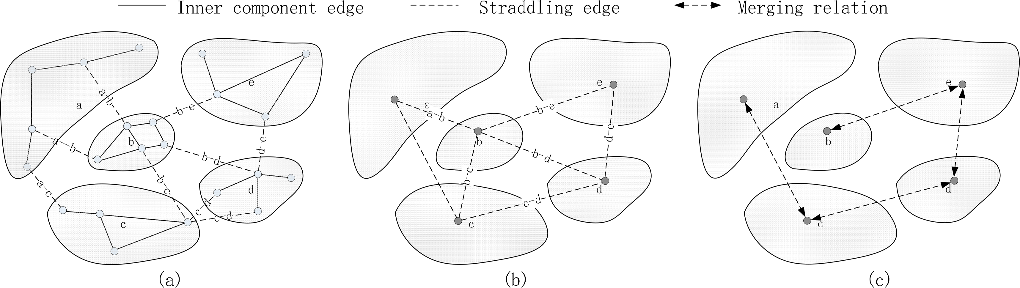
If the straddling edges are independent from the outcome of the inner component processing, the straddling edges can be processed in parallel. In this sense, the merging load is the sum of the weights of all the straddling edges in partitioning the SDDG. However, if the component linkages depend on the outcome of the inner component processing, multiple straddling edges between each pair of components should be merged into a new edge. In this situation, a graph of the components can be built with these edges. In Figure 3a, the straddling edges which straddle the same pair of components (i.e., edges with same labels) are merged into a new component edge (see Figure 3b). In this sense, the final result is achieved by merging any two connected components. As a matter of fact, if there are M components in this graph, only M – 1 times of merging are required to merge the results (see Figure 3c).
3.5. Implementation of a Thread-Level Parallel Engine for Scheduling the Kernel Functions
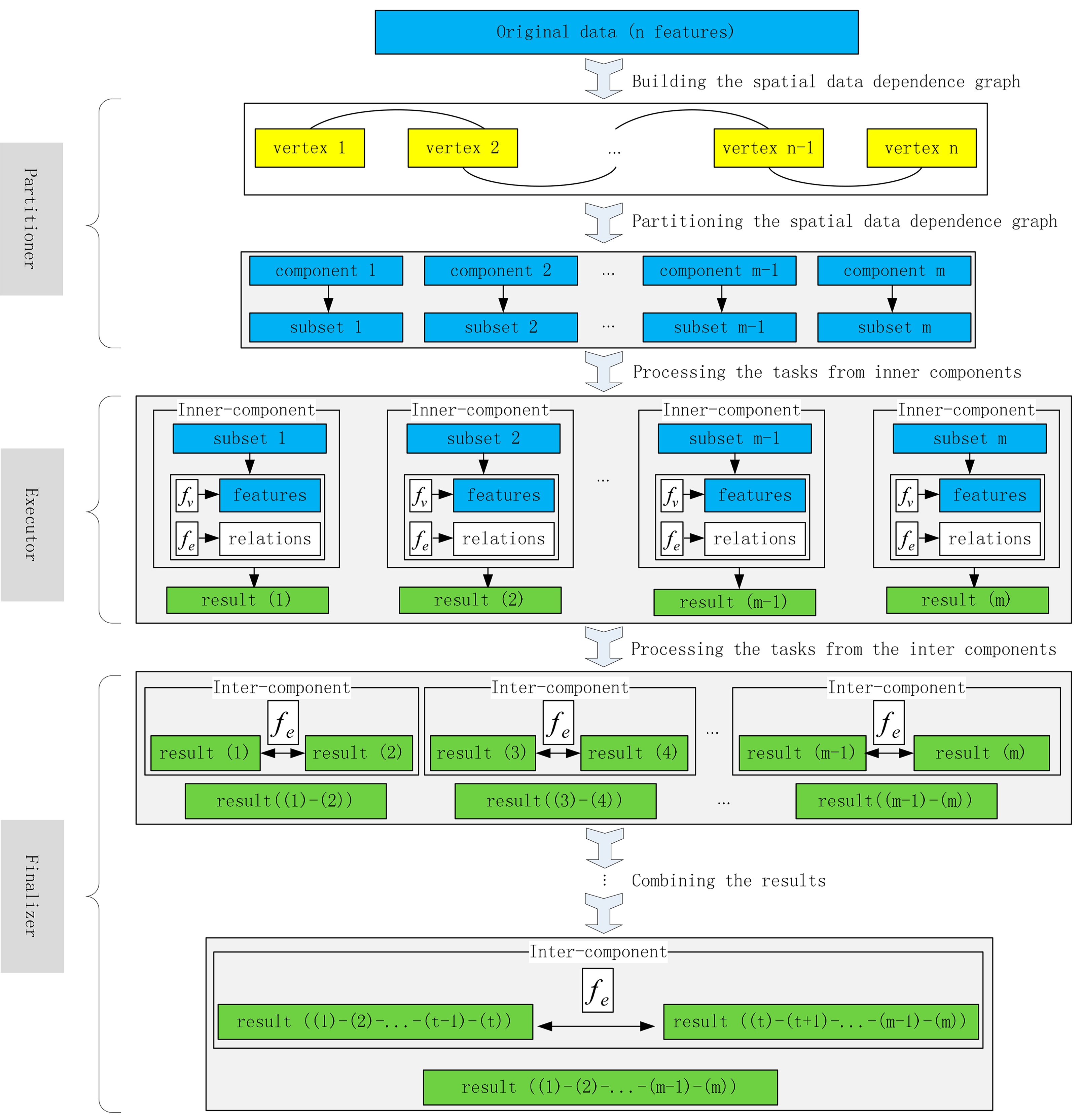
To drive the procedure of the spatial operations, a thread-level parallel engine is designed and developed (see Figure 4). The driving engine is composed of three modules: a task partitioner, an executor, and a finalizer. The partitioner takes charge of assigning the vector features into multiple subtasks. The executor manages a scalable computing thread pool for performing the vertex functions and edge functions from the inner-components. The parallel threads can simultaneously run without interaction. After all the subtasks are completed, the finalizer is called to handle the sub-results from inter-components through the edge functions iteratively. Moreover, multiple pairs of combinations in each iteration could be performed in parallel to reduce the merging time.
3.6. Computational Complexity
Transforming a spatial operation into SDDG version involves four steps: initializing SDDG, partitioning SDDG, performing the vertex functions and the edge functions in the thread pool, and finally merging the results. Therefore, the computational complexity can be modeled as follows:
4. Case Studies: Parallelization of the Buffer Operation and the Intersection Operation
The SDDG has been decided in Section 3 theoretically. To provide a practical understanding of the model for exploiting the parallelism, the detailed implementations of the buffer operation (see Section 4.2) and the intersection operation (see Section 4.3) are introduced. In Section 4.1, the data structure of the SDDG is firstly provided, and it is shared by different spatial operations. Secondly, the implementations of vertex functions, edge functions and the weight measurements for each operation are analyzed. Thus, the SDDG for an operation can be divided by the general partitioner (which was introduced in Section 3.3). Finally, each operation of SDDG version is submitted to the scheduling engine (see Section 3.5). The experiments and discussions are provided in Section 5. In GIS, Open Source software is gaining relevant market shares in academia, business, and public administration [71]. Fortunately and importantly, at least one open source project exists for all the different categories of geospatial software [72]. Typically, the GDAL/OGR library [73] provides the interoperability with the majority of common GIS data formats, and the GEOS library [74] offers basic geometry algorithms. Herein, GDAL-1.9.0 is selected to facilitate the reading and writing of vector data, and GEOS-3.4.2 is used to provide the spatial predicate functions.
4.1. The Structure of the SDDG
To build the SDDG for a spatial operation, the vertices and the edges should firstly be initialized. The weight of each vertex in the SDDG should be estimated according to the feature and the vertex function. For the buffer operation, the size of the feature provides an alternative measure for the computing intensity for the vertex. This is because performing the vertex function (the buffering algorithm) on the geometry of a feature with more points generally costs more time than that on a geometric feature with less points. Secondly, the weight of each SDDG edge is estimated according to source feature and target feature. For the intersection operation, the size of the two features is used to measure the computing intensity of that edge.
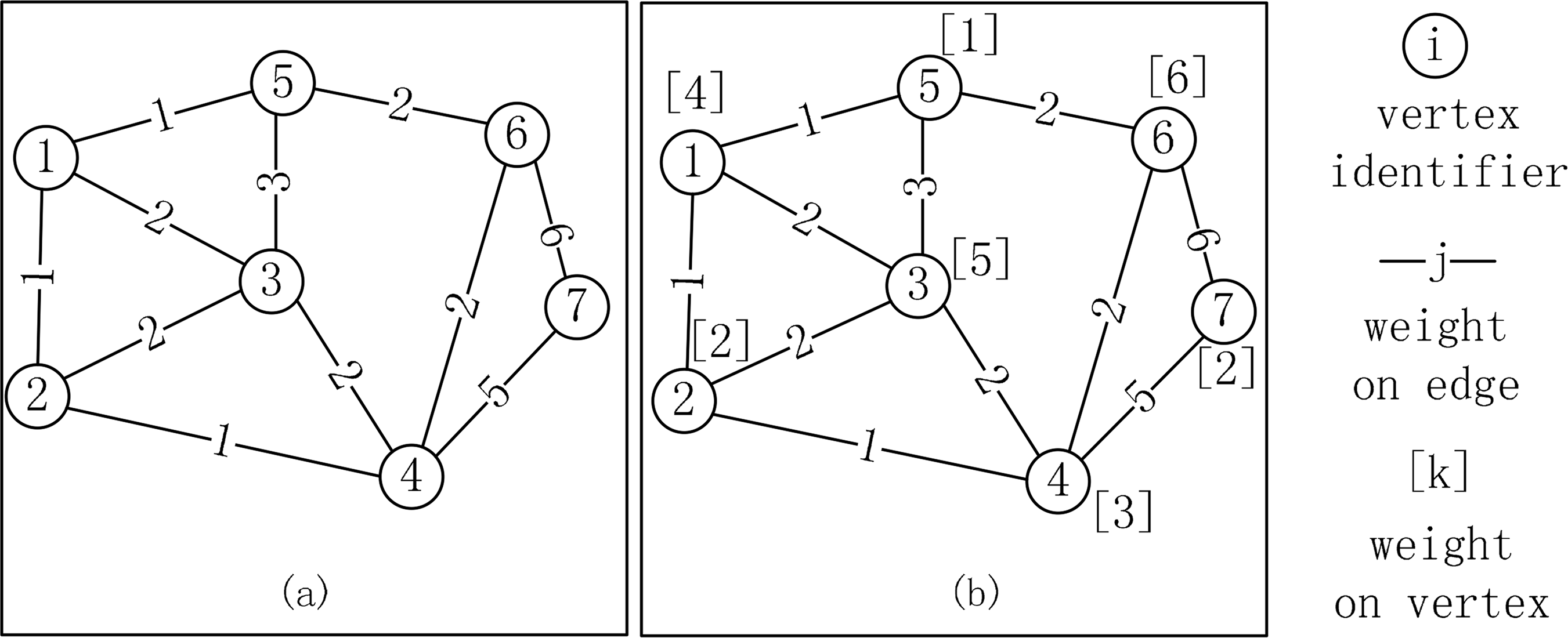
After the weights of all the vertices and edges are determined, a valid SDDG is initialized. To proceed, we firstly need to format the above information into the METIS format. Two types of weighted graphs in the METIS program are shown in Figure 5 (from [70]). The weights on the vertices and the edges can be used to represent computing intensities of the vertex function and the edge function in spatial operations. Moreover, representations of the buffer operation and intersection operation with SDDG need different types of graph, which will be shown in the following two sections.
4.2. Implementation of SDDG-BUFFER
To represent buffer operation with SDDG, each feature was represented as a vertex with a weight that can measure the computing intensity of the vertex function on the geometry of this feature. According to our experience, the working load of the vertex function for a feature is approximately proportional to the number of the points that constitutes the geometry of this feature. Therefore, the number of points is used as the vertex weight in buffer operation:
Herein, the vertex function and the edge function are realized respectively by calling the interfaces named Buffer() and Union()in GDAL supported with GEOS. It is obvious that the sequential function has been reused to realize the parallel version of the buffer operation.
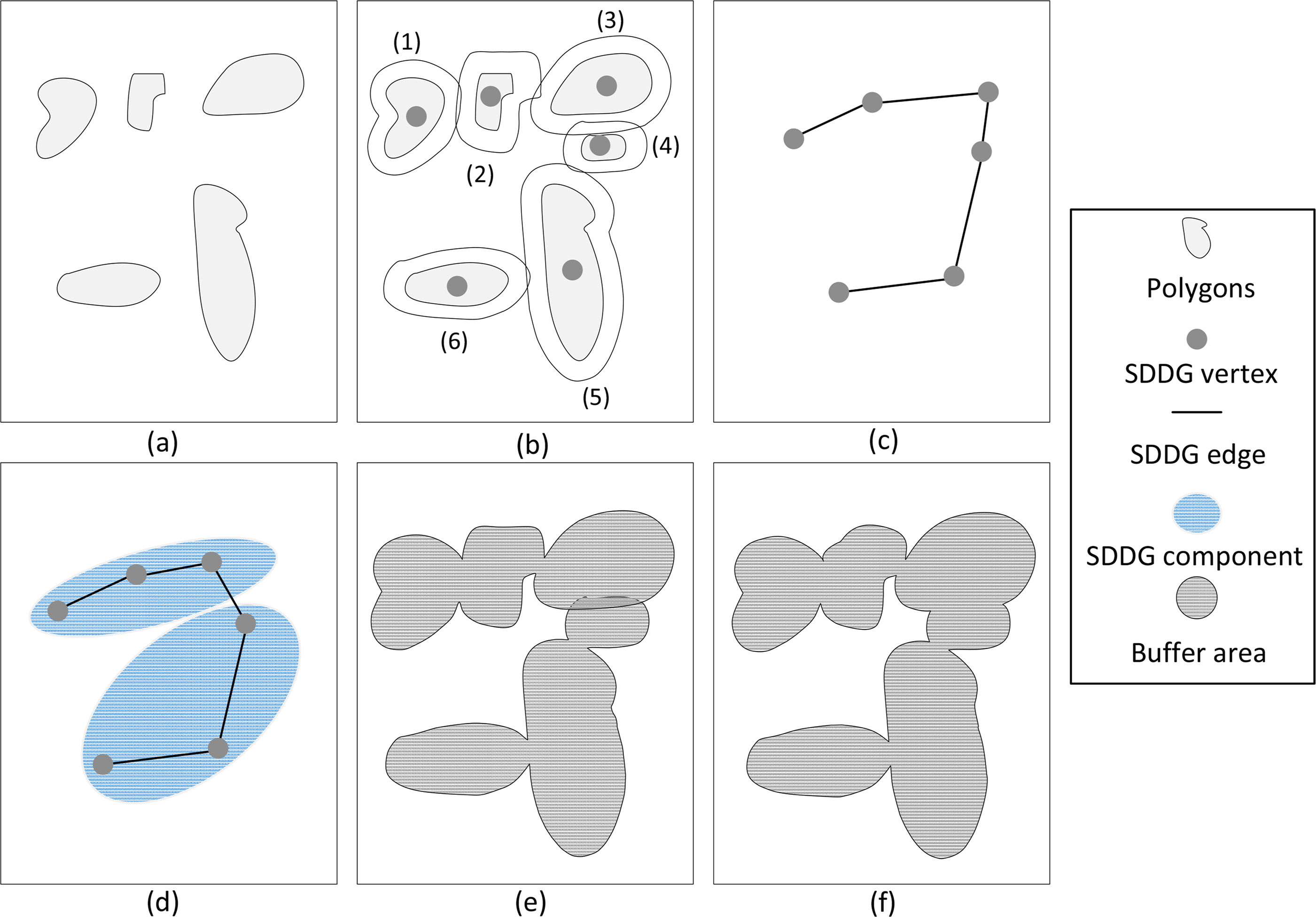
As shown in Figure 6 is the procedure of performing the buffer operation for six polygons (see Figure 6a) using the graph-based divide and conquer method. In Figure 6b, to speed up the process of building the distances edges for related geometries, a R-tree spatial index is used to search the polygons within a bounding box range, and an open source spatial indexing package called libspatialindex [75] is integrated. For each polygon in one layer, the bounding box is firstly calculated, and a spatial range query is used to search the polygons within a dissolving range. For each polygon, the bounding box is calculated firstly. Then, spatial range query is used to locate the possibly dissolving polygons with the bounding box expanded to twice the buffer width. The resulting polygons from this query should be further analyzed to determine the distance relations. For any pair of polygons with their exact distance less than or equal to twice the buffer width, a SDDG edge will be created (see Figure 6c).
The METIS package is used to decompose the SDDG into two components with the minimum number of edges that straddle, as shown in Figure 6d. More importantly, each component has an approximately equal computing load. After partitioning the SDDG, two subtasks are created. In Figure 6e, the two subtasks are performed simultaneously. In this step, the work denoted by the inner components is completed. Finally, the finalizer achieves the work denoted by the inter components through merging the sub-results (see Figure 6f).
4.3. Implementation of SDDG-INTERSECTION
To build the SDDG for the intersection operation, only the intersected geometries in two layers are selected and represented as vertices. As the computing intensity only exists for intersecting geometries, the computing weights should only be built for the edges, i.e., the weight of edge function. Therefore, the first type of METIS graph is used for representing the weights on edges. By this way, the geometries without intersected geometries are filtered out. As a matter of fact, performing the intersection of two larger geometries is more computationally intensive. Thus, the dot product of the sizes of the two geometries can measure the time complexity, and the same definition of the W(fe) like in Formula (6) is used. Herein, the edge function is realized by calling the interface named Intersection() in GDAL supported with GEOS. One another thing to note is that the vertex function fv is empty.
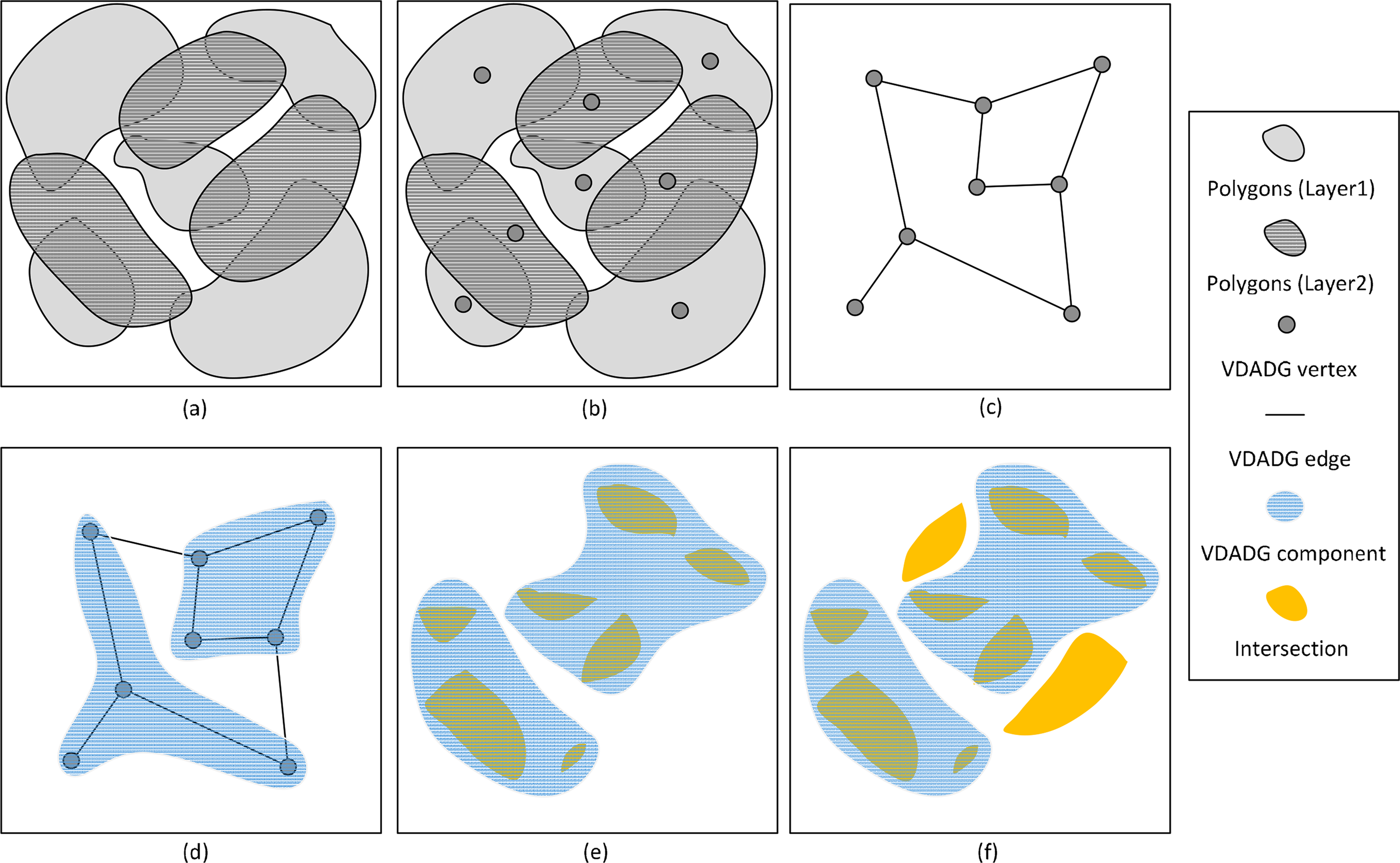
Figure 7 illustrates the procedure of performing the intersection operation for two polygon layers using the graph-based divide and conquer method. In Figure 7a, each polygon in one layer is topologically intersected with some polygons in another layer. All the polygons are represented by the SDDG vertices (see Figure 7b), and the SDDG edges are created for each pair of intersecting polygons (see Figure 7c). Similarly, to speed up the process of building the distance edges for related geometries in Figure 7b, the R-tree spatial index is also used to search the polygons within a bounding box range. For each polygon in one layer, the bounding box is firstly calculated. Then, spatial range query is used to locate the possibly intersecting polygons in another layer with that bounding box. This query can filter out most of the non-intersected geometries. All the result polygons from the query should be further analyzed to determine the topological relations.
As shown in Figure 7d, the METIS package is used to decompose the SDDG into two components with the minimum number of edges, which are straddled. After partitioning the SDDG, two subtasks are created. In Figure 7e, the two subtasks are performed simultaneously. In this step, the work denoted by the inner components is completed, and the result includes seven intersecting polygons. Finally, the finalizer achieves the work denoted by the inter components through intersecting the uncompleted intersected polygons (see Figure 7d).
5. Testing and Discussions
5.1. Testing Environment
The experimental environment is a Two-Way-Six-Core workstation running Microsoft Windows 7. It has two Six-Core Intel Xeon E5645 (2.40 GHz in each core), 64GB DDR3-1600 ECCSDRAM and 2TB hard disk (7200 rpm, 64MB cache). To leverage the power of multi-core processors, OpenMP is used for the thread-level parallelization. In addition, Hyper-Threading Technology makes a single physical processor appear as two logical processors, and the maximum number of threads for the two Six-Core Intel processors is 24. The program is developed in C++ language and compiled with Visual Studio 2010.
5.2. Testing Result of Buffer Operation
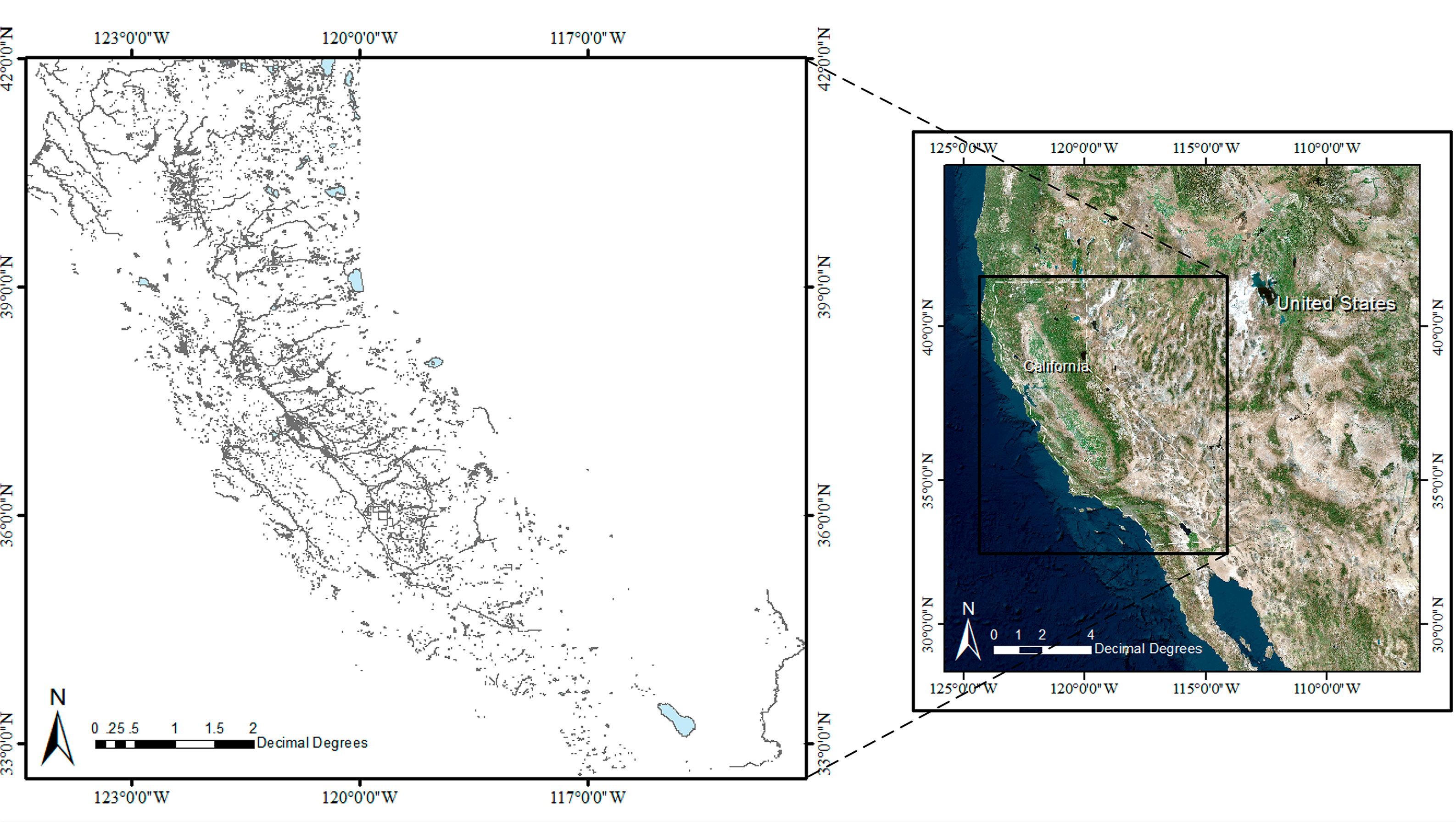
Figure 8 represents the dataset of water resource from California [76], and it contains 56177 polygon features. In addition, all the geometry errors have been corrected in ArcGIS 10.1 before processing. The spatial reference system for this dataset is World Geodetic System 1984 (WGS 84, EPSG: 4326).
The task is to generate buffer zones around each polygon feature with several widths, and the overlapping buffer zones should be dissolved. Firstly, a group of tests are performed in ArcGIS 10.1. Table 1 shows the computing time of the buffer operation in ArcGIS with five different buffer widths, and this group of tests is used to evaluate the accuracy of the results from the SDDG-BUFFER.
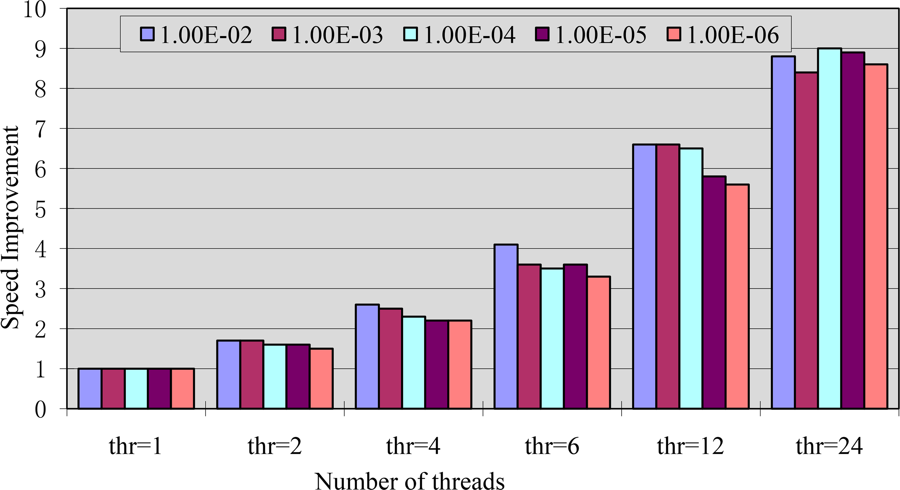
With the same data set, another group of tests in SDDG-BUFFER are performed with different parallel computing threads and five different buffer widths. As illustrated in Table 2, the computing time for each test is listed. Accordingly, the speed improvement for each test is calculated and shown in Figure 9. Moreover, the number of the output polygons varies when the buffer width changes. Obviously, a larger buffer width will need dissolving more proximate polygons, and thus, more computing time will be consumed. The dissolving percentage is used to quantitatively measure the influence of the buffer width, and it can be modeled by the following Formula:
With the increase of the number of the computing threads, the computing time reduced quickly. When the number of the computing threads is constant, a larger buffer width usually costs more time. As listed in Table 3, with the increase of the buffer width, the number of the output polygons reduced gradually, and this is consistent with the changes of the computing time. In comparison, the sequential SDDG-BUFFER (single thread) outperforms ArcGIS 10.1 in efficiency. In addition, parallel SDDG-BUFFER maintains a better scalability.
When performing the buffer operation, another parameter is used to control how many segments should be used to approximate a quadrant. Obviously, more segments will result in more vertices in the resulting buffer polygon, while fewer segments may reduce the accuracy of the output. This parameter in the ArcGIS 10.1 can’t be customized. When performing the buffer operation for a point feature in ArcGIS, 36 segments are generated. Thus, the number of segments for a quadrant herein is set to nine, and this can maintain a similar computing load and accuracy. To compare the results of ArcGIS and SDDG-BUFFER, their symmetric difference is performed, and the total area of the output polygons and the area of the symmetric difference are shown in Table 4. Then, the ratio between them can be calculated, and Table 4 suggests that the calculation errors of SDDG-BUFFER are very small and therefore can be ignored in our study. Moreover, for the same buffer width, the results of SDDG-BUFFER with different computing threads are identical, which verifies the correctness of SDDG-BUFFER.
5.3. Testing Result of Intersection Operation
The test data for the intersection operation includes two polygon datasets. The first data set contains 563133 land polygons [77] (Figure 10a), and the second data set contains 2461 polygons [78] (Figure 10b). The two datasets have the same spatial reference system, i.e., WGS 84. In addition, all the geometry errors have been previously corrected in ArcGIS 10.1.
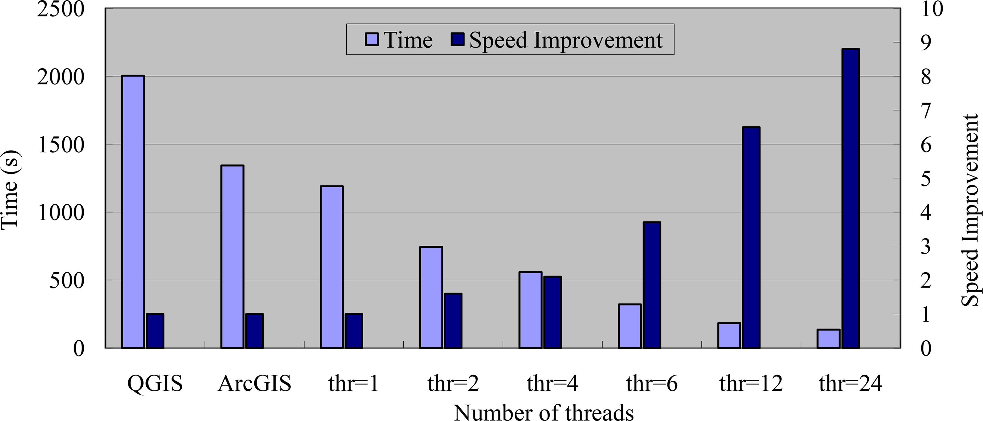
As illustrated in Figure 11, it took 2004 s to perform the intersection operation with the above vector layers in Quantum GIS 2.2-Valmiera (QGIS), and 1343 s to complete the same work in ArcGIS 10.1. After performing this operation, the common intersection contains 186038 polygon features as the output result. With 24 threads, SDDG-INTERSECT achieved a speed improvement of 8.8 times over the sequential version, and 14.7 times faster than QGIS, and 9.9 times faster than ArcGIS in performing the same work.
To compare the results of ArcGIS and QGIS, the symmetric difference is performed, and the output is empty. This shows that the accuracies of the results from these two software programs are extremely similar. Moreover, the results of SDDG-INTERSECT with different parallel computing threads are identical to those of QGIS, because their supporting libraries are identical. This also suggests the correctness of SDDG-INTERSECT.
5.4. Discussion
In this section, buffer operation and intersection operation were both tested in a multi-core computing environment. SDDG enabled the two GIS kernel functions to be partitioned into subtasks with the lowest possible merging cost. Each of the two parallel operations obtains an improved performance in a 12-core physical environment, and the computing performance outperforms the ArcGIS 10.1. The results have demonstrated the feasibility of our method. Moreover, the better reusability has demonstrated the high efficiency in developing parallel algorithms in comparison with a complete re-implementation of a spatial operation. In addition, the accuracy of the testing results have been assessed in the above two sections.
The distance relation in SDDG-BUFFER is considered a metric relation, while the intersecting relation in SDDG-INTERSECTION is considered a topological relationship. In fact, most of the spatial operations depend on these two categories of spatial relations. Therefore, SDDG in GDCMPSO provides a general method to parallelize the computationally intensive spatial operations. Moreover, the performance in GDCMPSO scales well, and no obvious bottlenecks have emerged with the increase in the participating threads.
In this paper, GDCMPSO is used to gain performance improvement for the buffer operation and the intersection operation in GeoCM. However, this method is not limited to GeoCM. According to the principle of the method in Section 3, two typical spatial operations are realized in Section 4. Experiments have suggested the great potential of this method for improving the spatial analysis on vector data. It is thus clear that if the spatial data dependence in a spatial operation can be represented by SDDG, this operation can be transformed to fit the graph-based divide and conquer method. However, an obvious limitation of this approach is that it is not suitable for decomposing individual geometries, and thus parallelism of spatial operations on individual geometries with heavy computing cost should be further exploited. Fortunately, this can be resolved by integrating the hierarchy into SDDG through expanding the graph vertex of a large feature to be a sub-graph. In other words, a large feature can be divided into small parts with adjacent relationships and then can be processed in nested parallel loops. Moreover, we are transforming the GDCMPSO from a standalone-computing node to a clustered computing environment, and we believe it will bring a greater efficiency improvement in the near future.
6. Conclusions
The proposed method, GDCMPSO, provides an effective way to exploit the parallelism for the spatial operations when processing massive geometric features. Particularly, the geometric features are represented as graph vertices (with vertex functions and vertex weights), the data dependence is represented as the graph edges (with edge functions and edge weights). Thus, the data partition is realized by graphs partitioning, and finally the spatial operations can be parallelized. The above steps form a complete solution to parallelizing spatial operations on vector data. The approach is used in parallelizing the buffer operation and the intersection operation. Experiments suggest that the proposed method is more operational and practicable than the existing methods for boosting the performance of the vector data processing. The proposed method mainly contributes to three aspects: (1) a theoretical method on how to exploit the parallelism for spatial operations on vector data; (2) the reusability of the existing software or packages; and (3) two parallelized spatial operations using the multi-core technology.
Acknowledgments
This work is supported by the National Natural Science Foundations of China (NSFC) under Grant 41371405 and the Basic Research Fund of Chinese Academy of Surveying and Mapping under Grant 7771413. We thank all the numerous scientists who released their code under Open Source licenses and made our method possible. We are also grateful to the anonymous reviewers for their helpful comments.
Author Contributions
Both authors contributed extensively to the work presented in this paper. Xiaochen Kang made the contribution on the programming, performing the experiments and writing the manuscript. Xiangguo Lin revised the manuscript extensively.
Conflicts of Interest
The authors declare no conflict of interest.
References
- ESRI (Environmental Systems Research Institute, Inc.). Spatial Operation Functions for St_Geometry. Available online: http://resources.arcgis.com/en/help/main/10.1/index.html#//006z00000020000000 (accessed on 7 May 2013).
- Egenhofer, M.J.; Glasgow, J.; Gunther, O.; Herring, J.R.; Peuquet, D.J. Progress in computational methods for representing geographical concepts. Int. J. Geogr. Inf. Sci 1999, 13, 775–796. [Google Scholar]
- Anselin, L. Gis research infrastructure for spatial analysis of real estate markets. J. House Res 1998, 9, 113–133. [Google Scholar]
- Opengis® Implementation Standard for Geographic Information—Simple Feature Access Part 2: Sql Option, 2010. Available online: http://portal.opengeospatial.org/files/?artifact_id=25354 (accessed on 16 March 2014).
- Sener, S.; Sener, E.; Nas, B.; Karagüzel, R. Combining AHP with GIS for landfill site selection: A case study in the Lake Beysehir catchment area (Konya, Turkey). Waste Manag 2010, 30, 2037–2046. [Google Scholar]
- Comber, A.J.; Sasaki, S.; Suzuki, H.; Brunsdon, C. A modified grouping genetic algorithm to select ambulance site locations. Int. J. Geogr. Inf. Sci 2011, 25, 807–823. [Google Scholar]
- Xiang, W.-N. A GIS method for riparian water quality buffer generation. Int. J. Geogr. Inf. Sci 1993, 7, 57–70. [Google Scholar]
- Li, L.; Wang, J.; Wang, C. Typhoon insurance pricing with spatial decision support tools. Int. J. Geogr. Inf. Sci 2005, 19, 363–384. [Google Scholar]
- Leung, Y.; Wong, M.H.; Wong, K.C.; Zhang, W.; Leung, K.S. A novel web-based system for tropical cyclone analysis and prediction. Int. J. Geogr. Inf. Sci 2012, 26, 75–97. [Google Scholar]
- Gui, D.; Lin, Z.; Zhang, C.; Liu, F. On the national geographical condition monitoring several strategic issues. In Proceedings of the 2012 International Archives of the Photogrammetry, Remote Sensing and Spatial Information Sciences, Melbourne, VIC, Australia, 25 August–1 September 2012; XXXIX-B4, pp. 539–541.
- Zhang, J.; Li, W.; Zhai, L. Understanding geographical conditions monitoring: A perspective from China. Int. J. Digit. Earth 2013. [Google Scholar] [CrossRef]
- Shekhar, S.; Gunturi, V.; Evans, M.R.; Yang, K. Spatial big-data challenges intersecting mobility and cloud computing. In Proceedings of the 2012 ACM International Workshop on Data Engineering for Wireless and Mobile Access, New York, NY, USA, 20 May 2012; pp. 1–6.
- Egenhofer, M.J.; Franzosa, R.D. Point-set topological spatial relations. Int. J. Geogr. Inf. Sci 1991, 5, 161–174. [Google Scholar]
- Palacio, M.P.; Sol, D.; González, J. Graph-based knowledge representation for GIS data. In Proceedings of the 2003 Mexican International Conference on Computer Science (ENC’03), Tlaxcala, Mexico, 8–12 September 2003; pp. 117–124.
- Xiong, B.; Oude Elberink, S.; Vosselman, G. A graph edit dictionary for correcting errors in roof topology graphs reconstructed from point clouds. ISPRS J. Photogramm. Remote Sens 2014, 93, 227–242. [Google Scholar]
- Tobler, W.R. A computer movie simulating urban growth in the Detroit Region. Econ. Geogr 1970, 234–240. [Google Scholar]
- Goodchild, M.F.; Longley, P.A. The practice of Geographic Information Science. In Handbook of Regional Science; Fischer, M.M., Nijkamp, P., Eds.; Springer: Berlin, Germany, 2014; pp. 1107–1122. [Google Scholar]
- Kang, X.; Liu, J.; Lin, X. Streaming progressive tin densification filter for airborne lidar point clouds using multi-core architectures. Remote Sens 2014, 6, 7212–7232. [Google Scholar]
- Lenoski, D.E.; Weber, W.-D. Scalable Shared-Memory Multiprocessing; Morgan Kaufmann Publishers: San Francisco, CA, USA, 1995. [Google Scholar]
- Guan, X.; Wu, H. Leveraging the power of multi-core platforms for large-scale geospatial data processing: Exemplified by generating dem from massive lidar point clouds. Comput. Geosci 2010, 36, 1276–1282. [Google Scholar]
- Dagum, L.; Menon, R. OpenMP: An industry standard API for shared-memory programming. IEEE. Comput. Sci. Eng 1998, 5, 46–55. [Google Scholar]
- Reinders, J. Intel Threading Building Blocks: Outfitting C++ for Multi-Core Processor Parallelism; O’Reilly Media, Inc.: Sebastopol, CA, USA, 2007. [Google Scholar]
- Openshaw, S.; Alvanides, S. Applying geocomputation to the analysis of spatial distributions. Geogr. Inf. Syst 1999, 1, 267–282. [Google Scholar]
- Clarke, K.C. Geocomputation’s future at the extremes: High performance computing and nanoclients. Parallel Comput 2003, 29, 1281–1295. [Google Scholar]
- Abrahart, R.J.; See, L.M. Geocomputation; Taylor & Francis: London, UK, 2014. [Google Scholar]
- Armstrong, M.P.; Marciano, R.J. Massively parallel strategies for local spatial interpolation. Comput. Geosci 1997, 23, 859–867. [Google Scholar]
- Wang, S. A cybergis framework for the synthesis of cyberinfrastructure, GIS, and spatial analysis. Ann. Assoc. Am. Geogr 2010, 100, 535–557. [Google Scholar]
- Huang, F.; Liu, D.; Tan, X.; Wang, J.; Chen, Y.; He, B. Explorations of the implementation of a parallel IDW interpolation algorithm in a Linux cluster-based parallel GIS. Comput. Geosci 2011, 37, 426–434. [Google Scholar]
- Armstrong, M.P.; Pavlik, C.E.; Marciano, R. Parallel processing of spatial statistics. Comput. Geosci 1994, 20, 91–104. [Google Scholar]
- Wang, S.; Armstrong, M.P. A theoretical approach to the use of cyberinfrastructure in geographical analysis. Int. J. Geogr. Inf. Sci 2009, 23, 169–193. [Google Scholar]
- Widener, M.J.; Crago, N.C.; Aldstadt, J. Developing a parallel computational implementation of amoeba. Int. J. Geogr. Inf. Sci 2012, 26, 1707–1723. [Google Scholar]
- Sorokine, A. Implementation of a parallel high-performance visualization technique in GRASS GIS. Comput. Geosci 2007, 33, 685–695. [Google Scholar]
- Zhao, Y.; Padmanabhan, A.; Wang, S. A parallel computing approach to viewshed analysis of large terrain data using graphics processing units. Int. J. Geogr. Inf. Sci 2013, 27, 363–384. [Google Scholar]
- Tabik, S.; Zapata, E.L.; Romero, L.F. Simultaneous computation of total viewshed on large high resolution grids. Int. J. Geogr. Inf. Sci 2013, 27, 804–814. [Google Scholar]
- Gong, Z.; Tang, W.; Bennett, D.A.; Thill, J.-C. Parallel agent-based simulation of individual-level spatial interactions within a multicore computing environment. Int. J. Geogr. Inf. Sci 2013, 27, 1152–1170. [Google Scholar]
- Burstedde, C.; Klauck, K.; Schadschneider, A.; Zittartz, J. Simulation of pedestrian dynamics using a two-dimensional cellular automaton. Phys. A 2001, 295, 507–525. [Google Scholar]
- Kang, X. Graph-based synchronous collaborative mapping. Geocarto Int 2014. [Google Scholar] [CrossRef]
- Wang, S.; Liu, Y. Teragrid GIScience gateway: Bridging cyberinfrastructure and GIScience. Int. J. Geogr. Inf. Sci 2009, 23, 631–656. [Google Scholar]
- Dowers, S.; Gittings, B.M.; Mineter, M.J. Towards a framework for high-performance geocomputation: Handling vector-topology within a distributed service environment. Comput. Environ. Urban. Syst 2000, 24, 471–486. [Google Scholar]
- Yang, C.; Raskin, R. Introduction to distributed geographic information processing research. Int. J. Geogr. Inf. Sci 2009, 23, 553–560. [Google Scholar]
- Zhang, T.; Tsou, M.-H. Developing a grid-enabled spatial web portal for Internet GIServices and geospatial cyberinfrastructure. Int. J. Geogr. Inf. Sci 2009, 23, 605–630. [Google Scholar]
- Yang, C.; Raskin, R.; Goodchild, M.; Gahegan, M. Geospatial cyberinfrastructure: Past, present and future. Comput. Environ. Urban. Syst 2010, 34, 264–277. [Google Scholar]
- Guan, Q.; Clarke, K.C. A general-purpose parallel raster processing programming library test application using a geographic cellular automata model. Int. J. Geogr. Inf. Sci 2010, 24, 695–722. [Google Scholar]
- Qin, C.-Z.; Zhan, L.-J.; Zhu, A.-X.; Zhou, C.-H. A strategy for raster-based geocomputation under different parallel computing platforms. Int. J. Geogr. Inf. Sci 2014, 1–18. [Google Scholar]
- Karypis, G.; Kumar, V. A fast and high quality multilevel scheme for partitioning irregular graphs. SIAM J. Sci. Comput 1998, 20, 359–392. [Google Scholar]
- Hennessy, J.L.; Patterson, D.A. Computer Architecture: A Quantitative Approach, 5th ed.; Morgan Kaufmann: San Fransisco, CA, USA, 2011. [Google Scholar]
- Bernstein, A.J. Analysis of programs for parallel processing. IEEE Trans. Comput 1966, 757–763. [Google Scholar]
- Kuck, D.J.; Kuhn, R.H.; Padua, D.A.; Leasure, B.; Wolfe, M. Dependence graphs and compiler optimizations. In Proceedings of the 8th ACM SIGPLAN-SIGACT Symposium on Principles of Programming Languages, Williamsburg, VA, USA, 26–28 January 1981; pp. 207–218.
- Maydan, D.E.; Hennessy, J.L.; Lam, M.S. Efficient and Exact Data Dependence Analysis; ACM SIGPLAN Notices: Toronto, ON, Canada, 1991; pp. 1–14. [Google Scholar]
- Li, Z.; Yew, P.-C.; Zhu, C.-Q. An efficient data dependence analysis for parallelizing compilers. IEEE Trans. Parallel Distrib. Syst 1990, 1, 26–34. [Google Scholar]
- Rau, B.R. Data flow and dependence analysis for instruction level parallelism. In Languages and Compilers for Parallel Computing; Springer: Berlin, Germany, 1992; Volume 589, pp. 236–250. [Google Scholar]
- Rundberg, P.; Stenström, P. An all-software thread-level data dependence speculation system for multiprocessors. J. Instruction-Level Parallelism 3.
- Adve, S.V.; Gharachorloo, K. Shared memory consistency models: A tutorial. Computer 1996, 29, 66–76. [Google Scholar]
- Lamport, L. How to make a multiprocessor computer that correctly executes multiprocess programs. IEEE Trans. Comput 1979, 100, 690–691. [Google Scholar]
- Haining, R.P. Spatial Data Analysis: Theory and Practice; Cambridge University Press: Cambridge, UK, 2003. [Google Scholar]
- Steiniger, S.; Hunter, A.J. The 2012 free and open source GIS software map—A guide to facilitate research, development, and adoption. Comput. Environ. Urban. Syst 2013, 39, 136–150. [Google Scholar]
- Lipton, R.J.; Tarjan, R.E. A separator theorem for planar graphs. SIAM J. Appl. Math 1979, 36, 177–189. [Google Scholar]
- Deconinck, S. The Algorithm Design Manual, 2nd ed; Springer-Verlag: New York, NY, USA, 2008. [Google Scholar]
- Andreev, K.; Racke, H. Balanced graph partitioning. Theor. Comput. Syst 2006, 39, 929–939. [Google Scholar]
- Hendrickson, B.; Kolda, T.G. Graph partitioning models for parallel computing. Parallel Comput 2000, 26, 1519–1534. [Google Scholar]
- Hendrickson, B.; Leland, R. An improved spectral graph partitioning algorithm for mapping parallel computations. SIAM J Sci Comput 1995, 16, 452–469. [Google Scholar]
- Miller, G.L.; Teng, S.-H.; Thurston, W.; Vavasis, S.A. Automatic Mesh Partitioning. In Graphs theory and Sparse Matrix Computation; George, A., Gilbert, J., Liu, J., Eds.; Springer-Verlag: New York, NY, USA, 1993; Volume 56, pp. 57–84. [Google Scholar]
- Nour-Omid, B.; Raefsky, A.; Lyzenga, G. Solving finite element equations on concurrent computers. In Proceedings of the 1986 Symposium on Parallel Computations and Their Impact on Mechanics, Boston, MA, USA, 13–18 December 1986; pp. 209–227.
- Miller, G.L.; Teng, S.-H.; Vavasis, S.A. A unified geometric approach to graph separators. In Proceedings of the 32nd Annual Symposium on Foundations of Computer Science, San Juan, Philippines, 1–4 October 1991; pp. 538–547.
- Garbers, J.; Promel, H.J.; Steger, A. Finding clusters in VLSI circuits. In Proceedings of the 1990 IEEE International Conference on Digest of Technical Papers, Santa Clara, CA, USA, 11–15 November 1990; pp. 520–523.
- Bui, T.N.; Jones, C. A Heuristic for Reducing Fill-in in Sparse Matrix Factorization; Parallel Processing for Scientific Computing: Philadelphia, PA, USA, 1993; pp. 445–452. [Google Scholar]
- Cheng, C.-K.; Wei, Y.-C. An improved two-way partitioning algorithm with stable performance [VLSI]. IEEE Trans. Comput. Aided Design Integr. Circuits Syst 1991, 10, 1502–1511. [Google Scholar]
- Hendrickson, B.; Leland, R.W. A multi-level algorithm for partitioning graphs. In Proceedings of the 1995 ACM/IEEE Conference on Supercomputing, New York, NY, USA, 4–8 December 1995; pp. 28–41.
- Metis-Serial Graph Partitioning and Fill-Reducing Matrix Ordering. Available online: http://glaros.dtc.umn.edu/gkhome/metis/metis/overview (accessed on 17 April 2014).
- Karypis, G.; Kumar, V. A Software Package for Partitioning Unstructured Graphs, Partitioning Meshes, and Computing Fill-Reducing Orderings of Sparse Matrices; University of Minnesota Department of Computer Science and Engineering, Army HPC Research Center: Minneapolis, MN, USA, 2013. [Google Scholar]
- Neteler, M.; Bowman, M.H.; Landa, M.; Metz, M. GRASS GIS: A multi-purpose open source GIS. Environ. Modell. Softw 2012, 31, 124–130. [Google Scholar]
- Steiniger, S.; Bocher, E. An overview on current free and open source desktop GIS developments. Int. J. Geogr. Inf. Sci 2009, 23, 1345–1370. [Google Scholar]
- GDAL-Geospatial Data Abstraction Library. Available online: http://www.gdal.org/ (accessed on 12 April 2014).
- GEOS-Geometry Engine, Open Source. Available online: http://trac.osgeo.org/geos/ (accessed on 22 March 2014).
- Libspatialindex. Available online: http://libspatialindex.github.iso (accessed on 7 March 2014).
- Download Openstreetmap Data for This Region: California. Available online: http://download.geofabrik.de/north-america/us/california.html (accessed on 2 April 2014).
- Openstreetmap Data. Available online: http://data.openstreetmapdata.com/land-polygons-split-4326.zip (accessed on 26 March, 2014).
- Geodata. Available online: http://www.subject.ch/geo/subject/data/layers/world/freegis_worlddata-0.2/geodata/ (accessed on 7 April 2014).


| Buffer Width (°) | 1.00E–06 | 1.00E–05 | 1.00E–04 | 1.00E-03 | 1.00E–02 |
|---|---|---|---|---|---|
| ArcGIS 10.1 | 3459 | 3497 | 3264 | 1682 | 22,995 |
| Buffer Width (°) | 1.00E–06 | 1.00E–05 | 1.00E–04 | 1.00E–03 | 1.00E–02 |
|---|---|---|---|---|---|
| No. of Threads | |||||
| 1 | 1530 | 1532 | 1564 | 1660 | 2471 |
| 2 | 1002 | 978 | 962 | 983 | 1434 |
| 4 | 703 | 683 | 671 | 669 | 956 |
| 6 | 457 | 429 | 449 | 465 | 608 |
| 12 | 271 | 265 | 242 | 230 | 374 |
| 24 | 178 | 172 | 174 | 198 | 282 |
| Buffer Width (°) | 1.00E–06 | 1.00E–05 | 1.00E–04 | 1.00E–03 | 1.00E–02 |
|---|---|---|---|---|---|
| Number of output polygons | 52,124 | 52,046 | 47,901 | 34,333 | 4199 |
| Dissolving percentage | 7.2% | 7.4% | 14.7% | 38.9% | 92.5% |
| Buffer Width (°) | 1.00E–06 | 1.00E–05 | 1.00E–04 | 1.00E–03 | 1.00E–02 |
|---|---|---|---|---|---|
| Comparing Items | |||||
| Total area of the output polygons | 0.649 | 0.654 | 0.705 | 1.269 | 9.558 |
| Area of the symmetric difference | 3.22E–09 | 2.12E–07 | 8.78E–06 | 6.29E–04 | 6.29E–03 |
| Ratio of the difference | 4.96E–09 | 3.24E–07 | 1.25E–05 | 4.96E–04 | 6.58E–04 |
© 2014 by the authors; licensee MDPI, Basel, Switzerland This article is an open access article distributed under the terms and conditions of the Creative Commons Attribution license (http://creativecommons.org/licenses/by/4.0/).
Share and Cite
Kang, X.; Lin, X. Graph-Based Divide and Conquer Method for Parallelizing Spatial Operations on Vector Data. Remote Sens. 2014, 6, 10107-10130. https://doi.org/10.3390/rs61010107
Kang X, Lin X. Graph-Based Divide and Conquer Method for Parallelizing Spatial Operations on Vector Data. Remote Sensing. 2014; 6(10):10107-10130. https://doi.org/10.3390/rs61010107
Chicago/Turabian StyleKang, Xiaochen, and Xiangguo Lin. 2014. "Graph-Based Divide and Conquer Method for Parallelizing Spatial Operations on Vector Data" Remote Sensing 6, no. 10: 10107-10130. https://doi.org/10.3390/rs61010107
APA StyleKang, X., & Lin, X. (2014). Graph-Based Divide and Conquer Method for Parallelizing Spatial Operations on Vector Data. Remote Sensing, 6(10), 10107-10130. https://doi.org/10.3390/rs61010107