Abstract
Diatoms are the major marine primary producers on the global scale and, recently, several methods have been developed to retrieve their abundance or dominance from satellite remote sensing data. In this work, we highlight the importance of the Southern Ocean (SO) in developing a global algorithm for diatom using an Abundance Based Approach (ABA). A large global in situ data set of phytoplankton pigments was compiled, particularly with more samples collected in the SO. We revised the ABA to take account of the information on the penetration depth (Zpd) and to improve the relationship between diatoms and total chlorophyll-a (TChla). The results showed that there is a distinct relationship between diatoms and TChla in the SO, and a new global model (ABAZpd) improved the estimation of diatoms abundance by 28% in the SO compared with the original ABA model. In addition, we developed a regional model for the SO which further improved the retrieval of diatoms by 17% compared with the global ABAZpd model. As a result, we found that diatom may be more abundant in the SO than previously thought. Linear trend analysis of diatom abundance using the regional model for the SO showed that there are statistically significant trends, both increasing and decreasing, in diatom abundance over the past eleven years in the region.1. Introduction
Phytoplankton is the basis of the marine food web and a key component in the marine ecosystem. The term phytoplankton functional type (PFT, see Table 1 for a list of abbreviations and symbols) is used to distinguish the different roles of the phytoplankton in the biogeochemical cycle of the oceans [1]. Of special interest are the diatoms, which are the major contributors to the oceanic primary production [2] and carbon export [3] and, together with dinoflagellates, the most diverse PFT [4,5]. Diatoms are also one of the largest PFTs in terms of size, ranging from micrometers to a few millimeters [4]. They tend to dominate the phytoplankton community in coastal, polar and upwelling regions, where waters are typically rich in nutrients. In the Southern Ocean (SO), they represent 89% of the primary production [2] and are found in high concentrations in stratified waters near ice edge-zones [6,7], but also frequently form blooms at the Polar Front [8].

Given the biogeochemical and ecological importance of diatoms, it is necessary to understand how they respond to climate variability on global and regional scales, a task that cannot be achieved without knowledge of their temporal and spatial distribution. In the last decade, considerable effort has been invested in developing and improving approaches to retrieve the global distribution of diatoms from satellite data. Examples of these are PHYSAT [9], PhytoDOAS [10] and the Abundance Based Approach (ABA) [1,11–13]. PHYSAT determines dominance of diatoms (in addition to nano-eukaryotes, Prochlorococcus, Synechocococus-like and Phaeocystis-like) by identifying their specific spectral signatures from the normalized water-leaving radiance. Like PHYSAT, PhytoDOAS is based on analyzing optical (hyperspectral) information of satellite data and retrieves diatoms (as well as cyanobacteria, dinoflagellates and coccolithophores) by identifying their specific absorption in the backscattered solar radiation. The ABA, such as that by Hirata et al. [1], in contrast, is an ecological approach which applies satellite-measured chlorophyll-a (Chla) to empirical relationships between TChla and diatoms (as well as dinoflagellates, green algae, haptophytes, prokaryotes, pico-eukaryotes and Prochlorococcus sp.) derived from in situ measurements. However, unlike PHYSAT, both PhytoDOAS and ABA provide a quantitative estimation of the diatom abundance instead of its dominance.
Compared to optically based approaches, a great advantage of the ABA is the smaller computational effort; even if the satellite data volume becomes larger with higher temporal and spatial resolutions, the data processing load is not heavy and re-processing can also be done relatively easily. The ABA can be applied to global level-2 or level-3 products of TChla, which are freely available to the scientific community, as opposed to, for example, PhytoDOAS method that uses the top of atmosphere radiance data (i.e., level-1 product). In addition, the ABA has better global coverage of in situ data for model development and validation. Because ABA is an empirical model, its refinement is needed in the light of additional data to improve the retrieval of diatoms for both global and under-sampled oceans.
This paper focus on the retrieval of diatom abundance of Hirata et al. [1] based on two premises: (i) Diatoms are the major primary producers in the SO [2] and (ii) 90% of the diffusely reflected irradiance measured by ocean color sensors originates from the first optical depth, also referred to as the penetration depth (Zpd) [14]. These premises are also general limitations of the existing ABA. Although Hirata et al. [1] used a large global data set of phytoplankton pigments, new measurements, particularly in the SO (defined here as the region south of 50°S), have become available since then. Main objectives of this paper are:
- (1).
Compilation of a new and larger global data set of in situ phytoplankton pigment profiles, including more measurements in the SO (Figure 1) which was not well covered previously, and to investigate the relationship between fractional contribution of diatoms and TChla using the new data set in comparison to previous findings.
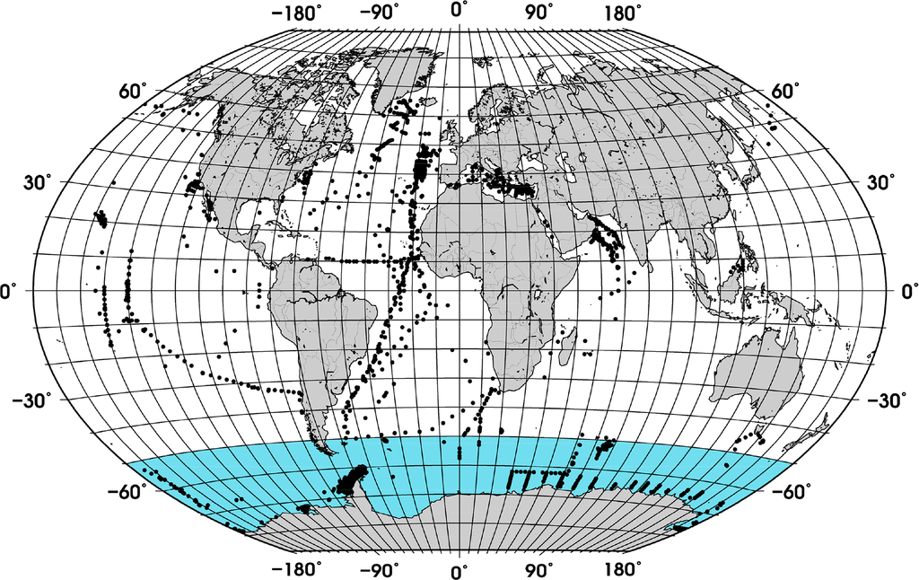 Figure 1. Distribution of the quality controlled in situ measurements. The SO, region south of 50°S, is the portion of the global ocean presented in blue.
- (2).
Refinement of the ABA to account for the pigment information in the Zpd (ABAZpd). In ABA [1], the fractional contribution of diatoms to TChla was estimated based on the previous work of Uitz et al. [15], who used the phytoplankton pigment concentration integrated over the euphotic depth (Zeu). However, the pigment concentration estimated by the satellite sensor is an optically-weighted concentration in the Zpd, which is approximately 4.6 times shallower than the Zeu [16].
- (3).
Evaluation of the performance of the ABA (i.e., ABAZpd) for global oceans and for the SO region.
The Theoretical Basis of the ABA
The ABA calculates the fraction (f) of Chla attributed to a specific PFT (f-PFT) using concentrations of diagnostic pigments of phytoplankton (i.e., Diagnostic Pigment Analysis–DPA, [15,17]). According to Uitz et al. [15], the Chla can be expressed by the sum of seven diagnostic pigments as:
For example, the fraction of Chla that is attributed to diatoms (f-Diatom) is derived as:
Once the f-PFT has been determined, the relationship between f-PFT and Chla can be represented by a model or fit function and quantified, where the relationship varies according to the PFT. The model for f-Diatoms was previously shown [1] as:
With the knowledge of the fit function, its parameters and Chla, it is possible to retrieve the f-Diatom, once Chla, which is operationally produced as a satellite product, is known. To retrieve the diatom abundance in terms of Chla (mg/m3), the f-Diatom is multiplied by the Chla value of each sample.
2. Data and Methods
2.1. In Situ Measurements of Phytoplankton Pigments
A data set of phytoplankton pigment profiles measured with the High-Performance Liquid Chromatography (HPLC) technique was supplemented with data obtained from the SeaWiFS Bio-optical Archive and Storage System (SeaBASS, [18]), Marine Ecosystem Data (MAREDAT, [19]), and from the individual cruises KEOPS ([20]), Bonus Good Hope, ANT-XVIII/2 (EisenEx), ANTXXI/3 (EIFEX, [3]), ANT XXVI/3, ANT XXVIII/3, Sonne SO218 [21], Merian 18-3, Meteor 55 and Meteor 60. The pigments from the cruises Meteor 55, Meteor 60, ANT XXVI/3 and ANT-XVIII/2 were measured in accordance with the method described in Hoffmann et al. [22] and for the cruises Merian 18-3 and ANT XXVIII/3 in accordance with that in Taylor et al. [23].
The data were quality controlled in a way similar to the method used by Uitz et al. [15] and Peloquin et al. [19]: (i) Samples with accessory pigment concentrations below 0.001 mg/m3 were set to zero, (ii) samples with TChla below 0.001 mg/m3 and fewer than 4 accessory pigments were excluded. The TChla was defined as the sum of monovinyl Chla, divinyl Chla, Chla allomers, Chla epimers and chlorophyllidae. To ensure that the profiles had a minimum vertical resolution, we restricted the data set to profiles with at least (i) one sample at the surface (0 to 12 m), (ii) one sample below the surface, (iii) samples collected at four or more different depths, and (iv) with one sample within the Zpd. The last quality control measure was based on the log10-linear relationship between TChlaZpd and the sum of all accessory pigments in the Zpd (TACCZpd). Data that fell outside the 95% confidence interval were removed.
In addition, samples located in coastal waters (<200 m) were excluded using the ETOPO1 bathymetry [24]. The final data set contained 3988 samples, which were randomly split into work (∼70% of the data) and validation (∼30% of the data) subsets (Figure 1). While the whole data set was used to calculate the partial coefficients used for estimating f-DiatomZpd, the work and validation subsets were used for model development and validation of the ABAZpd, respectively.
2.2. Satellite Data
Eleven years (2003–2013) of MODIS Aqua Level 3 4 km binned Chla data (R2013.0) were used. MODIS is a multispectral sensor on board of the Aqua satellite and with global coverage. The data were obtained from the OceanColor website [25] at daily temporal resolution. Monthly averages of diatom abundance were calculated onto a 10 minute grid and used to derive climatological maps of diatom abundance. To avoid coastal waters, where the retrieval of the ABA was not intended, we removed grid cells located in waters shallower than 200 m using the ETOPO1 bathymetry [24].
2.3. An Improved Abundance Based Approach
In previous approach [1], the f-Diatom was calculated using the coefficients of Uitz et al. [15], which take account of the phytoplankton pigment integrated over the Zeu. Here, we extended the ABA to take account of the information in the Zpd. For this purpose, we recalculated the coefficients a (Equation (1)) using an updated global data set of HPLC phytoplankton pigment profiles (N = 3988). The weighted pigment concentration in the Zpd (DPZpd) was calculated as described in Gordon & Clark [26], with the diffusive attenuation coefficient at 490 nm derived from the profiles of TChla as described in Morel & Maritorena [27]. The Zpd was computed as Zpd = Zeu/4.6, and Zeu was derived from the surface TChla as Zeu = 34 × TChla−0.39 (Morel, in Lee et al. [28]). Profiles were interpolated with 1-m increments from the deepest sample to the sample closest to the surface before the calculation of DPZpd.
A limitation of retrieving PFTs from HPLC pigments is the presence of a DP in more than one PFT [1,15]. The quality controlled data set was corrected for Fuco to account for its co-existence in other PFTs, in accordance with Hirata et al. [1].
Nonlinear minimization was used to retrieve the partial coefficients, which represent the estimates of the TChla to the DP ratios [15]. The function to be minimized is expressed as:
Using the new coefficients, the f-DiatomZpd was calculated for each sample of the work and validation subsets. The work subset was then sorted according to the TChlaZpd and smoothed with a 5-point running mean filter to improve the signal-to-noise ratio [1,12]. Next, the relationship between f-DiatomZpd and TChlaZpd was quantified using a nonlinear least-square fit applied to the work subset and represented by a model and its fitting parameters. Once the model has been defined, satellite-derived TChla data was applied to the model to obtain the global distribution of f-DiatomZpd. Diatom abundance (DiatomZpd, mg/m3) is then obtained by multiplying f-DiatomZpd by TChlaZpd.
The accuracy of the new model was tested using the validation subset. The uncertainties were estimated by the mean absolute error (MAE, [29]) and maximum absolute error (Max. Abs. Error) between the modeled and the measured (in situ) DiatomZpd. The models were compared by the difference between the MAE of the original model and the new model, relative to the original model, and expressed in percent (%). The data were log transformed prior to the calculation of the validation statistics. We used log10(data + λ) where λ = 0.00003, approximately one half of the smallest non-zero value of the in situ DiatomZpd validation data, since the data set contained zeroes. In addition, to investigate whether using different partial coefficients results in significant changes in f-Diatom, we estimated f-Diatom using the coefficients of Uitz et al. [15] and Brewin et al. [30] and compared the results based on the coefficient of determination.
A Regional Model for the SO
The main difference between the SO model and the global model is that the relationship between DiatomZpd and TChlaZpd is investigated not in terms of f-DiatomZpd, but instead in terms of the concentration of TChlaZpd that is attributed to diatoms, similar to the approach adopted by Brewin et al. [13] to retrieve phytoplankton size classes. As in Brewin et al. [13], the fit function was applied to log10-transformed data. To develop the regional model for the SO, we selected the samples of the global work and validation data sets that were located in the SO, creating a SO work and a validation data set with 1069 and 460 samples, respectively. The relationship between DiatomZpd and TChlaZpd was investigated and validated. Note that for the work data set we applied the running mean exclusively to the SO data.
2.4. Statistical Analysis of Trends
Linear trends were computed for February from monthly standardized anomalies over the 2003–2013 period in the SO using the regional model. To remove the seasonal cycle we calculated the monthly anomalies in diatom abundance for each grid cell by subtracting the climatological mean from the corresponding monthly mean (e.g., February 2003–climatology of February). The monthly anomalies were divided by the corresponding climatological standard deviation (e.g., standard deviation of February) to enable the direct comparison of trends between different regions (grid cells). The trends were computed using the non-parametric Kendall’s tau test with Sen’s method at the 95% confidence level and in grid cells with 100% temporal coverage.
3. Results and Discussion
3.1. The ABAZpd
Table 3 shows the partial regression coefficients, and their respective standard deviation, calculated with Equation (3). For comparison, we also present the partial coefficients estimated by Uitz et al. [15], Brewin et al. [30] and Fujiwara et al. [31]. Comparing our coefficients with those from Uitz et al. [15], there is a notable difference, except for the coefficients of Fuco and TChlb. These differences result from the inclusion of more profiles, their geographical distribution, the adjustment of Fuco prior to the DPA analysis, and because we used the pigment concentration weighted in the Zpd, while Uitz et al. [15] integrated the pigments over Zeu. When compared to the two other studies, where the partial coefficients were derived from surface measurements, our coefficients are more similar to those described in Brewin et al. [30]. Brewin et al. [30] included measurements of five Atlantic Meridional Transect (AMT) cruises in the Atlantic Ocean, while Fujiwara et al. [31] used measurements from three cruises in the Western Arctic Ocean. Although our data set includes measurements from these regions, the number of samples in the Arctic region is fewer than that from the Atlantic (Figure 1).
Moreover, we have re-run the analysis taking into consideration the surface samples (<12 m) from our profiles and observed only a slight difference in the coefficient of Fuco (1.531) as compared to the weighted Zpd concentrations. Except for Perid and Hexfuco, the standard deviation of our coefficients are much lower than, or similar to, the ones obtained by Uitz et al. [15].
Nonetheless, we observed very similar f-Diatom values when using the partial coefficients of Uitz et al. [15], Brewin et al. [30] and ours. The coefficients of determination are higher than 0.98, suggesting the choice of partial coefficients has no influence on the retrievals of f-Diatom, which is consistent with Brewin et al. [30]. Brewin et al. [30] compared size-fractionated chlorophyll (SFC) estimated from phytoplankton pigment data and calculated using Uitz et al. [15] partial coefficients and their own, with size-fractionated filtration (SFF) measurements. They observed biases between SFC and SFF for nanoplankton and picoplankton size classes; however, the variations in the partial coefficients did not influence the results significantly. The high correlation between the TChlaZpd and DPw, with DPw calculated using Equation (4) (r2 = 0.85, DPw = 0.86 TChlaZpd + 0.074, N = 3988, p < 0.001), gives us confidence to use the partial coefficients to determine the f-Diatom.
Figure 2 shows the change in the f-DiatomZpd with increasing TChlaZpd. The green and blue lines represent the new model (ABAZpd) and the model of Hirata et al. [1] (ABA*), respectively, parameterized with the DPZpd data set. The red line represents the original model and fitting parameters of Hirata et al. [1] (ABA**). It can be seen that diatoms are dominant at high TChlaZpd (Figures 2a,b), which is consistent with previous studies [1] even if a significant number of new samples were added in our dataset. Moreover, we also observed unusually high f-DiatomZpd in low TChlaZpd waters (<0.1 mg/m3, N = 670). Taking a closer look at the profiles, in which FucoZpd corresponded to at least 50% of the TACCZpd, we observed that most of the data sets (12 out of 16) are from samples taken in Antarctic, in the East Antarctic marginal ice zone (BROKE cruise, [6]). On average, the ratio of FucoZpd to TChlaZpd is 0.165 for the entire DPZpd data set, 0.071 excluding the SO data, but 0.317 for the SO data, indicating higher f-DiatomZpd values in low TChlaZpd waters in the SO.
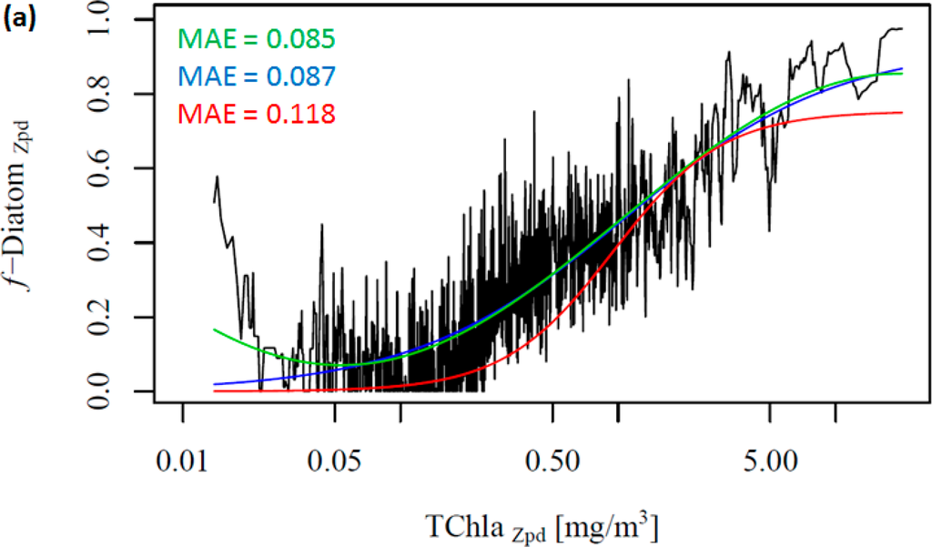
Considering our newer and larger data set, Hirata et al. [1] considerably underestimates f-DiatomZpd in almost the entire TChlaZpd range (Figure 2a-red line). This is partly due to the difference in the data set used. When we fit their model to the new data set, the model is found to fit well to the data, as indicated by the low errors (Table 5 and Figure 2a-blue line). However, it fails when predicting f-DiatomZpd in very low TChlaZpd waters, mostly for the SO. Thus, we test a new model, a sinusoidal function to better fit this observed trend in the SO (Table 4, Figure 2-green line). The ABAZpd and ABA* produce almost identical curves for TChlaZpd above 0.065 mg/m3 and similar fitting and validation statistics. The ABA** model provides accurate retrieval of diatoms globally. However, it produces larger errors than the ABAZpd and the ABA* do for the SO. The ABAZpd improves the MAE by 27.96% for the SO (Table 6 and Figure S1).
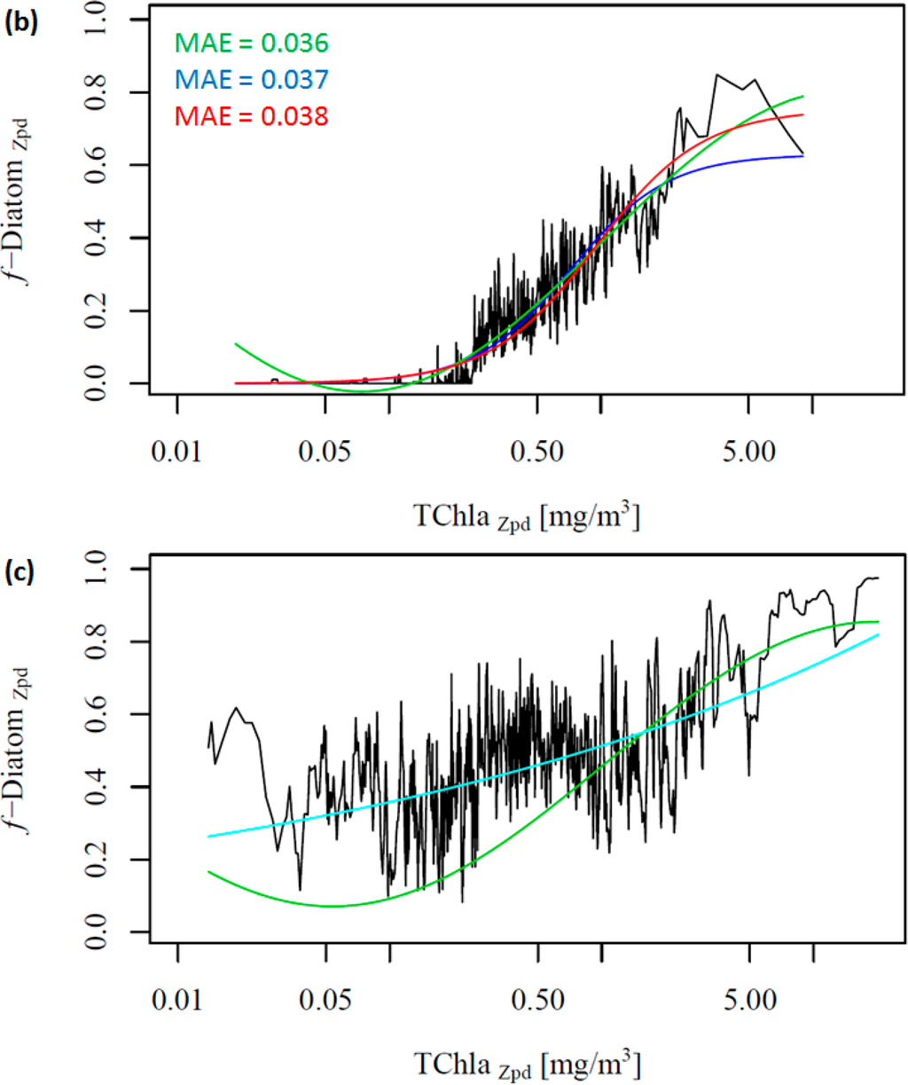
To further investigate the influence of the SO data, we removed these data from the work data set (38% of the data), recalculated f-DiatomZpd, and fitted the models (Figure 2b and Table 4). The comparison of Figure 2a,b shows clearly the influence of the SO data, which is responsible for most of the data spread in Figure 2a as well as for the high f-DiatomZpd in low TChlaZpd waters. When we exclude the SO data from the analysis, the fits improve greatly the MAE decrease to values close to 0.04 (Table 5). In addition, it leads to a better representation of the diatom abundance in oligotrophic waters, as well as to an underestimation of the actual f-DiatomZpd in the SO, as shown in Figure 3. The advantage of including the SO data is a more realistic retrieval of diatoms in the SO, but an overestimation in other regions of low TChlaZpd. While the in situ data show that the f-DiatomZpd might be very low (∼0) at very low TChlaZpd (e.g., in oligotrophic gyres), the predicted f-DiatomZpd presents values higher than zero, overestimating f-DiatomZpd in the oligotrophic gyres.
It should be noted that the model used to retrieve f-DiatomZpd as a function of TChlaZpd was empirically built upon in situ data sets, which showed that diatoms tend to be the dominant PFT at high TChla. However, this may not be the case of blooms of mixed PFTs occur, or with a different PFT (e.g., coccolithophores close to New Zealand [32]), as pointed out by Brewin et al. [13]. In such cases, additional information on PFTs derived from methods that do not depend on this assumption (e.g., PhytoDOAS) may improve the knowledge on the diatom abundance and the distribution pattern.
Moreover, we did not obtain significant results in fitting the two global models to the SO data exclusively (Figure 2c, ABAZpd plotted as reference). The diatoms in the SO exhibit a variability which is different from other oceanic regions (e.g., the North Pacific and the North Atlantic), and there is a need for a regional SO model. Thus, we developed a regional model for the SO, and the relationship between TChlaZpd and DiatomZpd in the SO can be expressed as: log10(y) = 1.1559log10(x) + (−0.2901) (Figure S2 in the Supplementary Information). The validation results of the SO model show that the regional model is consistent and more appropriate than the global ABAZpd model for retrieving diatoms in the SO (Table 6 and Figure S2 in the Supplementary Information). The regional model improved by 17% the retrieval of diatoms abundance in the SO compared with the ABAZpd.
The ideal global retrieval of diatoms should apply the ABAZpd model parameterized with the global data set excluding SO data (Figure 2b green line) to the region north of 50°S, and regional SO model for waters south of 50°S. These two models presented overall the lowest fitting and validation errors for the corresponding regions. This approach would not only provide more accurate retrievals of diatoms in the SO, but also overcome the overestimation of the global ABAZpd model in oligotrophic waters. However, applying two models generated a non-negligible offset between the SO and adjacent oceans (result not shown).
3.2. Satellite Retrieval of Diatoms Using ABAZpd
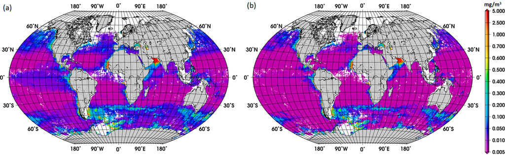
Acknowledging the uncertainties of the satellite Chla product, we first assessed the difference between the satellite retrievals of diatom abundance using the ABAZpd and the original ABA, for the SO and global oceans. As expected from the previous findings (Figure 2a), we observed that, on average, higher abundances of diatoms were retrieved with the ABAZpd than with the original ABA for the entire 2003–2013 period. For the SO, the concentration of diatoms calculated using the global ABAZpd is 0.074 mg/m3 and for the global oceans 0.070 mg/m3. In contrast, estimates of diatoms with the original ABA are 0.049 and 0.050 mg/m3, respectively. For comparison, the concentration of diatoms using the regional SO model is larger, 0.117 mg/m3. This evidence of the enhanced abundance of diatoms retrieved from the global ABAZpd model and from the regional SO model suggests that the production and export of carbon to the deep ocean might be larger than previously expected in the SO.
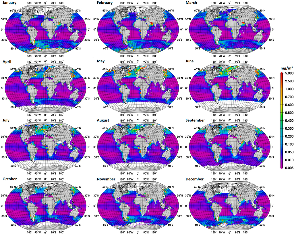
The new global climatology of diatom abundance is presented in Figure 4. The climatology for the SO is presented in the Supplementary Information (Figure S3). The general distribution of the global diatom abundance is in line with current knowledge on the distribution of diatoms, i.e., higher concentrations of diatoms in the upwelling and coastal regions. Low concentrations of diatoms are observed in oligotrophic waters of the subtropical gyres and in high-nutrient low-chlorophyll (HNLC) waters, such as regions in the SO where waters are rich in macronutrients but are lacking in iron. There is also a clear seasonal cycle in the polar regions, with diatoms reaching the highest concentrations during their respective summer months, which is also observed in the climatology for the SO. Among other important patterns is the increase in diatom concentration from December to February and in September in the Arabian Sea. These observed patterns are associated with the Northeast (NE) and Southwest (SW) monsoons, respectively. According to Garrison et al. [33], the monsoon seasons are generally characterized by increased concentrations of diatoms, thus our result shows a consistency with the previous in situ study too.
The climatology mostly covers the spatial variability, within a limited temporal range, whereas the trend gives information for a longer period, and both are important information for the understanding of ocean biogeochemistry. The spatial variability of the linear trends of diatom abundance in the SO is high, and no significant trend was observed for most of the sub regions of the SO (results not shown). The overall the trend for the SO was 0.036 (dimensionless) (standard deviation = 12.84, p-value = 0.019). Clearly, a more detailed analysis is needed to investigate the main driving forces behind these trends.
4. Conclusions
In conclusion, we have shown that the original ABA underestimates the diatom abundance in the Southern Ocean (SO). Our investigation revealed that diatoms in the SO might be more abundant than previous thought, possibly because (1) the lack of in situ phytoplankton pigment data, and that (2) the relationship between TChla and the f-Diatom in the SO is distinct from the global relationship.
We have developed a new global and regional ABAZpd that significantly improve the representativeness of the retrievals in the SO. The mean absolute error (MAE) declined from 0.776 to 0.559 using the global ABAZpd, improving by 28% the estimation of diatoms in the SO. The regional model further improved the MAE by 17% (MAE = 0.465) compared with the global ABAZpd model. This was achieved by re-evaluating the ABA using a large data set of global phytoplankton pigment profiles spanning 24 years (1988–2012). Additionally, the ABA was further improved by considering the information in the Zpd.
We have shown that the ideal global retrieval of diatoms combines the ABAZpd model fitted to the data set (excluding SO data, MAE = 0.883) with the regional SO model. However, applying two models generates an offset between the oceans, thus selective use of the global and the SO algorithms may be necessary depending on the objective of the application.
Satellite retrievals of PFTs are a useful tool for identifying and quantifying their presence in the oceans and in this study we have advanced our knowledge on the retrieval of diatoms from space by identifying limitations and developing improvements. Future studies should focus on optimizing the ABA method also for other PFTs.
Supplementary Information
remotesensing-06-10089-s001.pdfAcknowledgments
We would like to thank all principal investigators and contributors for collecting the in situ data available in SeaBASS, MAREDAT, Lter database, BonusGoodHope project (LOV, Josephine Ras, Amelie Tale, Herve Claustre), KEOPS cruise (Herve Claustre) and from the other individual cruises mentioned in this paper. Data from the Palmer LTER data repository were supported by Office of Polar Programs, NSF Grants OPP-9011927, OPP-9632763 and OPP-0217282. We are also thankful to Werner Wosnok for the statistical advice and Marc Taylor for discussions. We acknowledge the Ocean Biology Processing Group of NASA and the NASA Goddard Space Flight Center's Ocean Data Processing System (ODPS) for the production and distribution of the MODIS data. We would like to thank the three anonymous reviewers, whose comments lead to a significantly improved manuscript. The present study was funded by the Helmholtz Association via the project Helmholtz-University Young Investigators Group PHYTOOPTICS in cooperation with the Institute of Environmental Physics (University Bremen), by the Total Foundation Group via project Phytoscope and by the Japan Aerospace Exploration Agency (JAXA) via the project Global Observation Mission-Climate. The first author is funded by the CAPES, Brazil, by the research grant BEX 3483/09-6.
Author Contributions
Mariana Soppa led the study, performed data analysis and wrote the draft version of the manuscript. Takafumi Hirata and Astrid Bracher supervised the work. Brenner Silva and Tilman Dinter contributed in statistical support and programming. Ilka Peeken provided the pigment data sets collected during ANT XVIII/2, ANT XXVI/3, ANT XXI/3, Meteor 55, Meteor 60 and Sonja Wiegmann was involved with laboratory analysis and sampling of ANT XXVIII/3, Sonne SO218, Merian 18-3 phytoplankton pigment data. All co-authors assisted in writing the manuscript.
Conflicts of Interest
The authors declare no conflict of interest.
References and Notes
- Hirata, T.; Hardman-Mountford, N. J.; Brewin, R.J.W.; Aiken, J.; Barlow, R.; Suzuki, K.; Isada, T.; Howell, E.; Hashioka, T.; Noguchi-Aita, M.; et al. Synoptic relationships between surface Chlorophyll-a and diagnostic pigments specific to phytoplankton functional types. Biogeosciences 2011, 8, 311–327. [Google Scholar]
- Rousseaux, C.S.; Gregg, W.W. Interannual variation in phytoplankton primary production at a global scale. Remote Sens 2014, 6, 1–19. [Google Scholar]
- Smetacek, V.; Klass, C.; Strass, V.H.; Assmy, P.; Montresor, M.; Cisewski, B.; Savoye, N.; Webb, A.; d’Ovidio, F.; et al. Deep carbon export from a Southern Ocean iron-fertilized diatom bloom. Nature 2012, 487, 313–319. [Google Scholar]
- Armbrust, E.V. The life of diatoms in the world’s oceans. Nature 2009, 459, 185–192. [Google Scholar]
- Leblanc, K.; Aristegui, J.; Armand, L.; Assmy, P.; Beker, B.; Bode, A.; Breton, E.; Cornet, V.; Gibson, J.; Gosselin, M.-P.; et al. A global diatom database—Abundance, biovolume and biomass in the world ocean. Earth Syst. Sci. Data 2012, 4, 149–165. [Google Scholar]
- Wright, S.W.; van den Enden, R.L. Phytoplankton community structure and stocks in the East Antarctic marginal ice zone (BROKE survey, January–March 1996) determined by CHEMTAX analysis of HPLC pigment signatures. Deep-Sea Res Pt II-Top St Oce 2000, 47, 2363–2400. [Google Scholar]
- Arrigo, K.R.; Robinson, D.H.; Worthen, D.L.; Dunbar, R.B.; DiTullio, G.R.; VanWoert, M.; Lizotte, M.P. Phytoplankton community structure and the drawdown of nutrients and CO2 in the Southern Ocean. Science 1999, 283, 365–367. [Google Scholar]
- Bracher, A.U.; Kroon, B.M.A.; Lucas, M.I. Primary production, physiological state and composition of phytoplankton in the Atlantic Sector of the Southern Ocean. Mar Ecol Prog Ser 1999, 190, 1–16. [Google Scholar]
- Alvain, S.; Moulin, C.; Dandonneau, Y.; Bréon, F.M. Remote sensing of phytoplankton groups in case 1 waters from global SeaWiFS imagery. Deep-Sea Res Pt I-Oceanog Res 2005, 52, 1989–2004. [Google Scholar]
- Bracher, A.; Vountas, M.; Dinter, T.; Burrows, J.P.; Röttgers, R.; Peeken, I. Quantitative observation of cyanobacteria and diatoms from space using PhytoDOAS on SCIAMACHY data. Biogeosciences 2009, 6, 751–764. [Google Scholar]
- Devred, E.; Sathyendranath, S.; Stuart, V.; Maass, H.; Ulloa, O.; Platt, T. A two-component model of phytoplankton absorption in the open ocean: Theory and applications. J Geophys Res-Oceans 2006, 111. [Google Scholar] [CrossRef]
- Hirata, T.; Aiken, J.; Hardman-Mountford, N.; Smyth, T.J.; Barlow, R.G. An absorption model to determine phytoplankton size classes from satellite ocean colour. Remote Sens Environ 2008, 112, 3153–3159. [Google Scholar]
- Brewin, R.J.W; Sathyendranath, S.; Hirata, T.; Lavender, S.J.; Barciela, R.M.; Hardman-Mountford, N.J. A three-component model of phytoplankton size class for the Atlantic Ocean. Ecol Model 2010, 221, 1472–1483. [Google Scholar]
- Gordon, H.R.; Mccluney, W.R. Estimation of depth of sunlight penetration in sea for remote sensing. Appl Opt 1975, 14, 413–416. [Google Scholar]
- Uitz, J.; Claustre, H.; Morel, A.; Hooker, S.B. Vertical distribution of phytoplankton communities in open ocean: An assessment based on surface chlorophyll. J Geophys Res-Oceans 2006, 111. [Google Scholar] [CrossRef]
- Hyde, K.J.W.; O’Reilly, J.E.; Oviatt, C.A. Validation of SeaWiFS chlorophyll a in Massachusetts Bay. Cont Shelf Res 2007, 27, 1677–1691. [Google Scholar]
- Vidussi, F.; Claustre, H.; Manca, B.B.; Luchetta, A.; Marty, J.C. Phytoplankton pigment distribution in relation to upper thermocline circulation in the eastern Mediterranean Sea during winter. J Geophys Res-Oceans 2001, 106, 19939–19956. [Google Scholar]
- Werdell, P.J.; Bailey, S.; Fargion, G.; Pietras, C.; Knobelspiesse, K.; Feldman, G.; McClain, C. Unique data repository facilitates ocean color satellite validation. EOS Trans AGU 2003, 84, 377–387. [Google Scholar]
- Peloquin, J.; Swan, C.; Gruber, N.; Vogt, M.; Claustre, H.; Ras, J.; Uitz, J.; Barlow, R.; Behrenfeld, M.; Bidigare, R. The MAREDAT global database of high performance liquid chromatography marine pigment measurements. Earth Syst Sci Data 2013, 5, 109–123. [Google Scholar]
- Uitz, J.; Claustre, H.; Griffiths, F.B.; Ras, J.; Garcia, N.; Sandroni, V. A phytoplankton class-specific primary production model applied to the Kerguelen Islands region (Southern Ocean). Deep-Sea Res Pt I-Oceanog Res 2009, 56, 541–560. [Google Scholar]
- Cheah, W.; Taylor, B.B.; Wiegmann, S.; Raimund, S.; Krahmann, G.; Quack, B.; Bracher, A. Photophysiological state of natural phytoplankton communities in the South China Sea and Sulu Sea. Biogeosciences Discuss 2013, 10, 12115–12153. [Google Scholar]
- Hoffmann, L.; Peeken, I.; Lochte, K.; Assmy, P.; Veldhuis, M. Different reactions of Southern Ocean phytoplankton size classes to iron fertilization. Limnol Oceanogr 2006, 51, 1217–1229. [Google Scholar]
- Taylor, B.B.; Torrecilla, E.; Bernhardt, A.; Taylor, M.H.; Peeken, I.; Röttgers, R.; Piera, J.; Bracher, A. Bio-optical provinces in the eastern Atlantic Ocean and their biogeographical relevance. Biogeosciences Discuss 2011, 8, 3609–3629. [Google Scholar]
- Amante, C; Eakins, B.W. Etopo1 1 ARC-Minute Global Relief Model: Procedures, Data Sources and Analysis; U S Government: Washington DC, USA, 2009; p. 19. [Google Scholar]
- OceanColor Web. Available online: http://oceancolor.gsfc.nasa.gov/ (acessed on 10 February 2014).
- Gordon, H.R.; Clark, D.K. Remote sensing optical-properties of a stratified ocean: An improved interpretation. Appl Opt 1980, 19, 3428–3430. [Google Scholar]
- Morel, A.; Maritorena, S. Bio-optical properties of oceanic waters: A reappraisal. J Geophys Res-Oceans 2001, 106, 7163–7180. [Google Scholar]
- Lee, Z.; Du, K.; Arnone, R.; Liew, S.; Penta, B. Penetration of solar radiation in the upper ocean: A numerical model for oceanic and coastal waters. J Geophys Res-Oceans 2005, 110. [Google Scholar] [CrossRef]
- Willmott, C.J.; Matsuura, K. Advantages of the mean absolute error (MAE) over the root mean square error (RMSE) in assessing average model performance. Clim Res 2005, 30, 79–82. [Google Scholar]
- Brewin, R.J.; Sathyendranath, S.; Lange, P.K.; Tilstone, G. Comparison of two methods to derive the size-structure of natural populations of phytoplankton. Deep-Sea Res Pt I-Oceanog Res 2014, 85, 72–79. [Google Scholar]
- Fujiwara, A.; Hirawake, T.; Suzuki, K.; Imai, I.; Saitoh, S.I. Timing of sea ice retreat can alter phytoplankton community structure in the western Arctic Ocean. Biogeosciences 2014, 11, 1705–1716. [Google Scholar]
- Sadeghi, A.; Dinter, T.; Vountas, M.; Taylor, B.; Peeken, I.; Altenburg Soppa, M.; Bracher, A. Improvement to the PhytoDOAS method for identification of coccolithophores using hyper-spectral satellite data. Ocean Sci 2012, 8, 1055–1070. [Google Scholar]
- Garrison, D.L.; Gowing, M.M.; Hughes, M.P.; Campbell, L.; Caron, D.A.; Dennett, M.R.; Shalapyonok, A.; Olson, R.J.; Landry, M.R.; Brown, S.L.; et al. Microbial food web structure in the Arabian Sea: A US JGOFS study. Deep-Sea Res Pt II-Top St Oce 2000, 47, 1387–1422. [Google Scholar]
© 2014 by the authors; licensee MDPI, Basel, Switzerland This article is an open access article distributed under the terms and conditions of the Creative Commons Attribution license (http://creativecommons.org/licenses/by/4.0/).