Non-Vegetated Playa Morphodynamics Using Multi-Temporal Landsat Imagery in a Semi-Arid Endorheic Basin: Salar de Uyuni, Bolivia


Abstract
: Playas in endorheic basins are of environmental value and highly scientific because of their natural habitats of a wide variety of species and indicators for climatic changes and tectonic activities within continents. Remote sensing, due to its capability of acquiring repetitive data with synoptic coverage, provides a unique tool to monitor and collect spatial information about playas. Most studies have concentrated on evaporite mineral distribution using remote sensing techniques but research about grain size distribution and geomorphologic changes in playas has been rarely reported. We analysed playa morphodynamics using Landsat time series data in a semi-arid endorheic basin, Salar de Uyuni in Bolivia. The spectral libraries explaining the relationship between surface reflectance and surficial materials are extracted from the Landsat image on 11 November 2012, the collected samples in the area and the precipitation data. Such spectral libraries are then applied to the classification of the other Landsat images from 1985–2011 using maximum likelihood classifier. Four types of surficial materials on the playa are identified: salty surface, silt-rich surface, clay-rich surface and pure salt. The silt-rich surface is related to crevasse splays and river banks while the clay-rich surface is associated with floodplain and channel depressions. The classification results show that the silt-rich surface tends to have a positive relationship with annual precipitation, whereas the salty surface negatively correlates with annual precipitation and there is no correlation between clay-rich surface and annual precipitation. Salty surfaces seem to consist primarily of clay due to their similar characteristics in response to precipitation changes. The classification results also show the development of a crevasse splay and avulsions. The results demonstrate the potential of Landsat imagery to determine the grain size and sedimentary facies distribution on playas in endorheic basins.1. Introduction
As a common feature of internal drainage basins, playas are vital for understanding the natural habitats of endemic microbes, plants and animals [1] and for interpreting the interrelation between climate and tectonic activity within continents [2]. Studies also proved that playas sediments could be potential hydrocarbon reservoirs [3], as they may contain significant numbers of thin fluvial sheetflood deposits. Many researchers have suggested that a framework for surface sedimentary facies or depositional environments is needed in playas [4–7]. Over the past decades, a number of studies have applied remote sensing techniques to study playas and have demonstrated the usefulness of remote sensing in such studies (e.g., [1,2,8–15]). However, most of these studies have focused on mapping evaporite minerals and water bodies. There are few studies focusing on grain size and sedimentary facies distribution using remote sensing [10,16–20], mostly due to difficult accessibility [2,18] and hazardous environments during peak discharge events [21]. In this paper, we analyse playa morphodynamics by Landsat time series data in the semi-arid endorheic (internal drainage basin) basin of the Salar de Uyuni in Bolivia.
A basic theory about the relationship between sediment and reflectance is used in this paper. If the sediment is very coarse, the porosity is high and thus the scatter effect is strong and the reflectance is low. The high porosity also indicates a high capacity for storing water. As grain size decreases, the water content simultaneously decreases due to a decline in porosity. When the sediment is fine sand or silt, the reflectance is high due to little scattering effect and a large specific area. However, with an increasing content of clay, the capacity of the sediment for storing water increases because of the large internal surface, which is related to adhesive, cohesive and osmotic forces [22]. Due to strong evapo-transpiration in the study area (1500 mm/year), the water in the sediments precipitates salt in the long dry period (normally from April to November in the study area). When the surface is covered by salt it has a strong reflectance, while for clay-rich areas, the reflectance is low due to soil moisture. In addition, crust cracking at clay-rich surface reinforces its roughness and therefore contributes to a low reflectance.
This study documents the use of Landsat imagery in combination with precipitation data and field investigation to analyse playa morphodynamics. First, we establish the relationship between the various types of sediments (e.g., salt-, sand- and clay-rich sediments) and spectral reflectance, and then build spectral libraries for each type. Such spectral libraries are then used to classify the Landsat time series data from 1985–2011 over the study area, with Maximum Likelihood Classification (MLC) method being used as a supervised classifier. Then, we analyse the relationships between different classes and sedimentary facies, and investigate the changes of these classes in combination with precipitation data. Finally, we analyse the geomorphological changes with a time series of classified maps.
2. Study Area
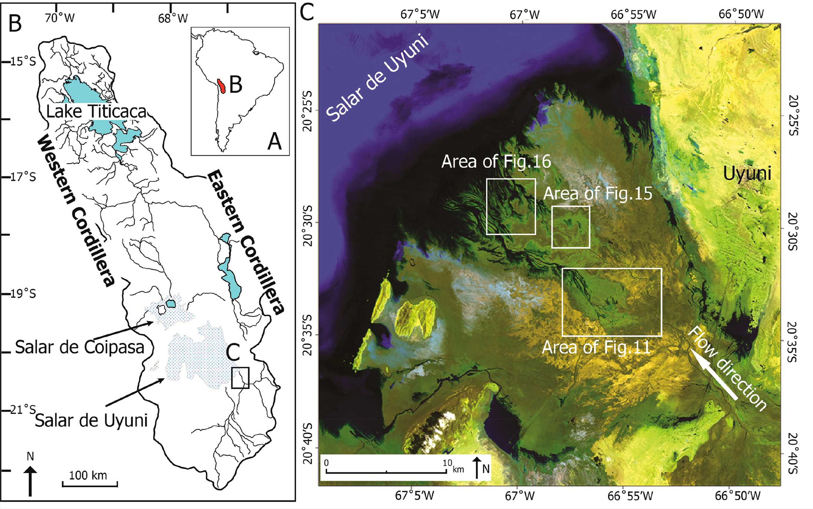
The study area is at the southeast edge of the world’s largest salt lake, Salar de Uyuni, Bolivia, with an area of 10,582 km2 and it is at an elevation of 3656 meters above mean sea level (Figure 1). It is located in the southern part of the Altiplano Basin. The basin formed as part of the Andean ocean-continent convergent margin with eastward subduction of the oceanic Nazca Plate beneath the continental South American Plate [23,24]. The central Andes developed eastward during the Cenozoic and regional horizontal shortening led to increasing thickness of the continental crust [25,26]. The Altiplano Basin, an endorheic basin, is filled with Tertiary to Quaternary fluvial and lacustrine sediments and volcaniclastic deposits [27,28].
The Altiplano Basin has a semi-arid climate with an annual precipitation of more than 800 mm in the north and less than 200 mm in the south [30] and an evapo-transpiration potential of 1500 mm [31,32]. Precipitation shows this clear-cut north-to-south decrease in Altiplano plateau due to the low pressure systems of the Altiplano, strong low-level north-westerly winds with warm, moist, unstable air flow along the eastern flank of the central Andes giving rise to convection precipitation. Moreover, pole-ward low-level air flow helps to maintain the intense convection [33]. The rainy season in the study area is from December to March, and the average annual rainfall is about 185 mm, which is greatly exceeded by potential evapo-transpiration. With SE-to-NW flow direction, the Río Colorado is one of the main inflow rivers for the Salar de Uyuni. In this study, we focus on the terminus of Río Colorado river system, where human interference is limited.
3. Data Acquisition
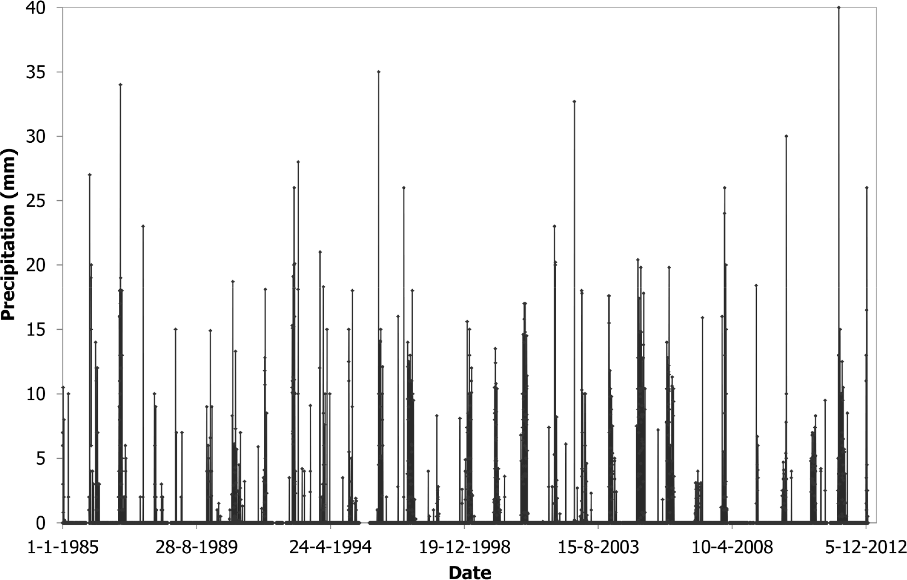
Daily precipitation data were available over the study area for the period 1985–2012 from the Bolivian Servicio Nacional de Meteorología e Hidrología (Figure 2). Using the precipitation datasets from three meteorological stations in the study area over the period 1980–2010, Li et al. [21] has demonstrated that the rainfall distribution in Uyuni is spatially consistent with those of other meteorological stations using the double mass curve technique. This implies that such daily precipitation data in Uyuni can be considered representative of the whole study area. The field survey was carried out from 13–18 November 2012 before the rainy season. The field sampling sites were determined using Landsat ETM+ imagery and land cover samples were collected with geo-located GPS.
Landsat Surface Reflectance Climate Data Record (CDR) data was collected from the USGS website. The surface reflectance CDR, including many Landsat TM and all ETM+ scenes, is a high-level Landsat data product and is derived from specialised software called Landsat Ecosystem Disturbance Adaptive Processing System (LEDAPS). The surface reflectance data were available in the form of 16-bit signed integer with the range of −2000 to 16,000. The studied river terminus is included entirely within Landsat path 233, row 74. Thanks to the available daily precipitation data, we accurately determined the rainy and dry periods of 1985–2012. This allowed us to select Landsat images in the dry periods (Table 1).
4. Methodology
4.1 Landsat CDR Data Pre-Processing
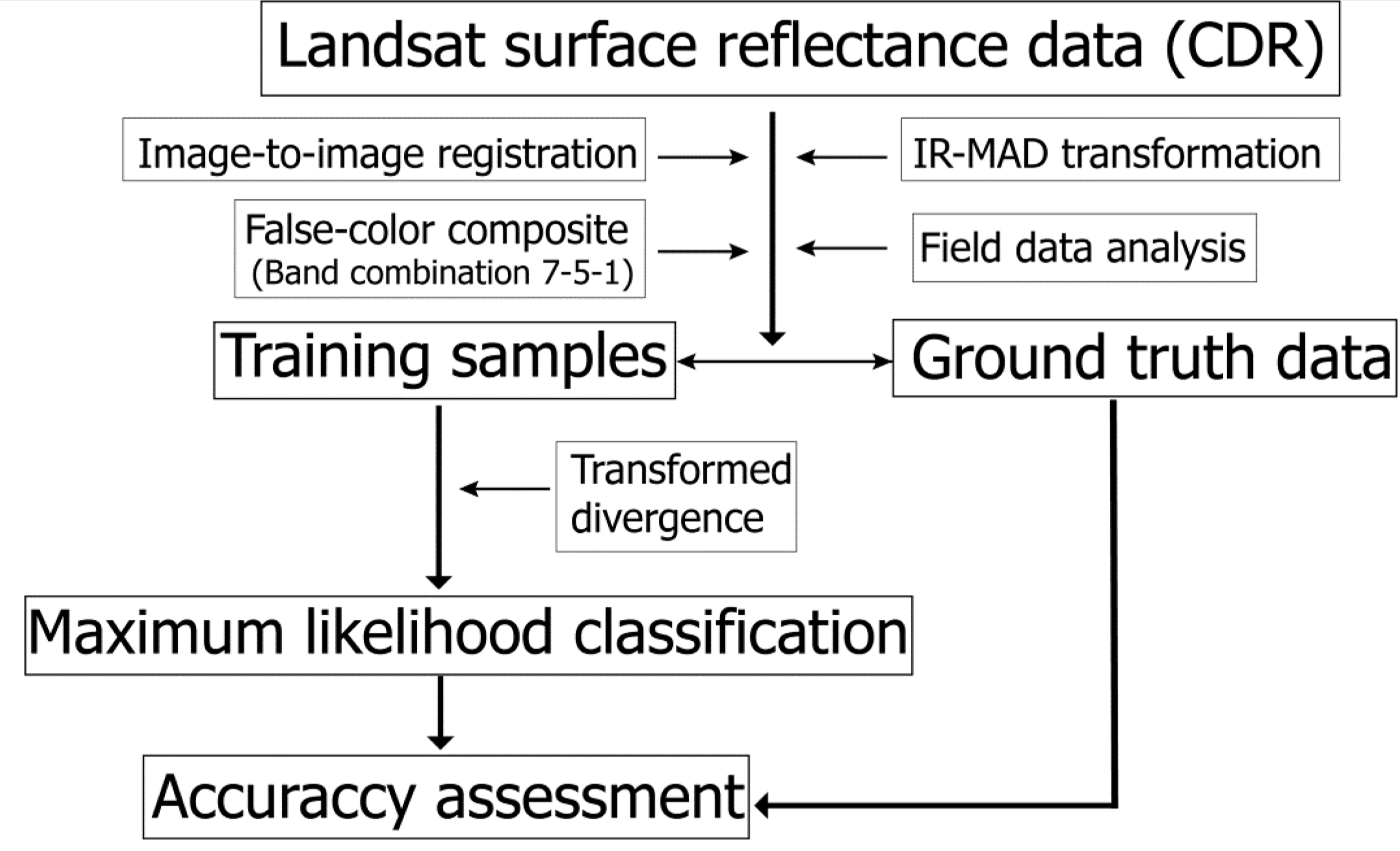
As seen in Figure 3, first of all, image-to-image registration is done to make sure that a certain pixel covers the same area in all the images. The Landsat surface reflectance data are then normalized with Iteratively Reweighted Multivariate Alteration Detection (IR-MAD) transformation to eliminate the unwanted effects due to illumination variation for different dates, although, surface reflectance data as used in this study (Landsat CDR) are supposed to be corrected for such effects which implies that such normalizations may not be strictly required [34]. The false-color composite of the base image in combination with field data analysis were used to select training samples. Prior to classification, it is necessary to check the separability of the target classes. This has been done using the transformed divergence technique, where a low value between two classes indicates similarities between them and hence difficulties in distinguishing two distinct classes by the classifier. The maximum likelihood classifier was then applied for the classification. This is a well-known approach that has been frequently used for classification in semi-arid environments [35–37]. The accuracy assessment of the approach was evaluated by different metrics including overall accuracy, kappa coefficient, producer’s accuracy and user’s accuracy. More detailed explanation of the methodology will be given in the following subsections.
Spectral libraries of different classes (end-members) were built using the Landsat image on 11 November 2012 and ground truth data collected during the field campaign (Figure 3). This image was selected as the base image since this is the closest date corresponding to the ground measurements and there was no TM image available for this year. Bands with a low fraction of saturated pixels have been selected for later normalisation and classification. In this paper, we used three Landsat bands 2, 4 and 7, which have low fractions of saturated pixels for the period 1985–2011 according to digital number statistics of all bands. All these selected bands were subsequently normalized to a referenced image with IR-MAD transformation [38]. The IR-MAD requires a full dataset since it uses the spatial data over the entire scene for the normalization. Therefore, the ETM image of 2012 due to the missing lines (Scan Line Corrector (SLC) failure) cannot be used and we have taken the TM image of 2011 as the reference image for normalization of the other images. This might introduce error into the analysis, however, since the data are surface reflectance (Landsat CDR data) that is supposed to be corrected for illumination, sensor-related and other effects, this error will not be significant over such a homogeneous area. Moreover, the high coefficients of determination (mean R2 > 0.95) indicated strong correlations between the reference image and targeted images.
4.2 Training Samples Selection and Analysis
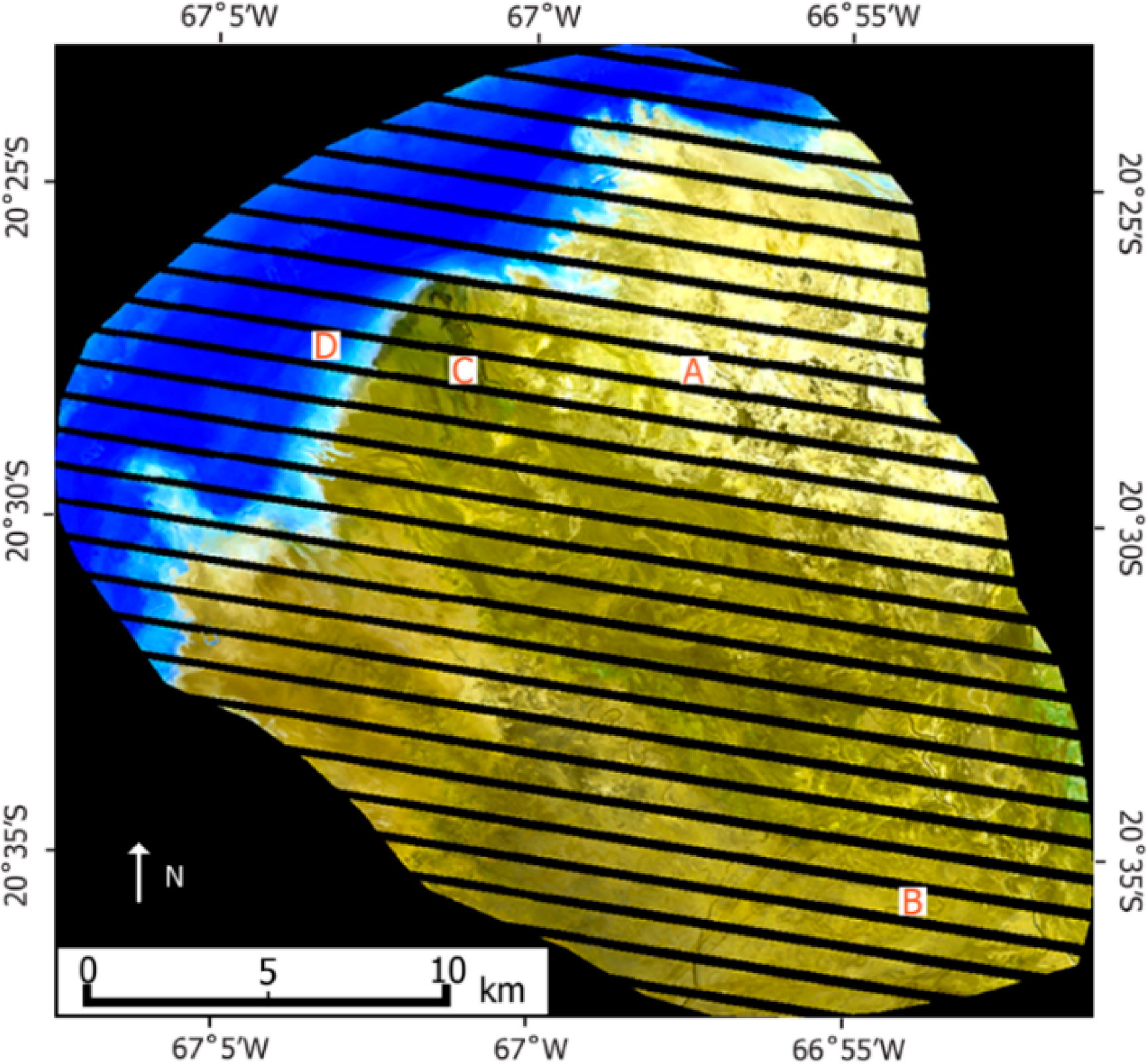
The training samples were selected from a false-color composite image and field sampling data. We used false-color composites of band 7 (2.08–2.35 µm), band 5 (1.55–1.75 µm) and band 1 (0.45–0.52 µm) (Figure 4) to differentiate different surface materials (in particular clay-rich and silt-rich surface). Since both bands 5 and 7 are located in the near-infrared region, they are sensitive to soil moisture and indicate water absorption regions. We identified four surface materials: A, B, C and D (Figure 4).
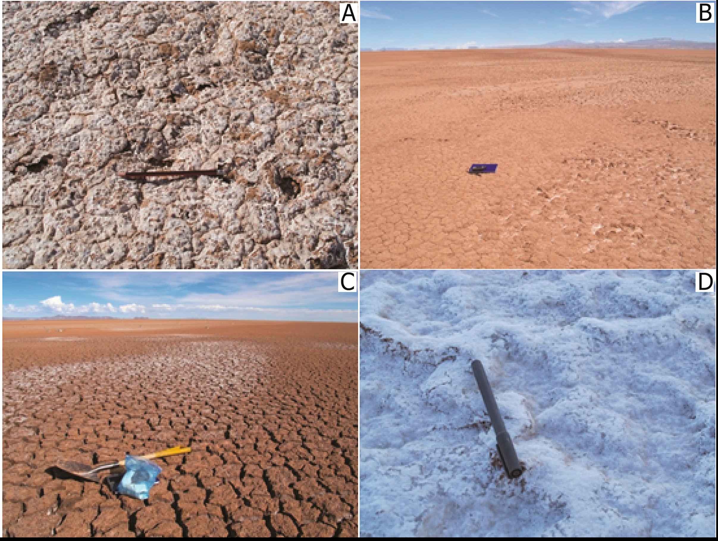
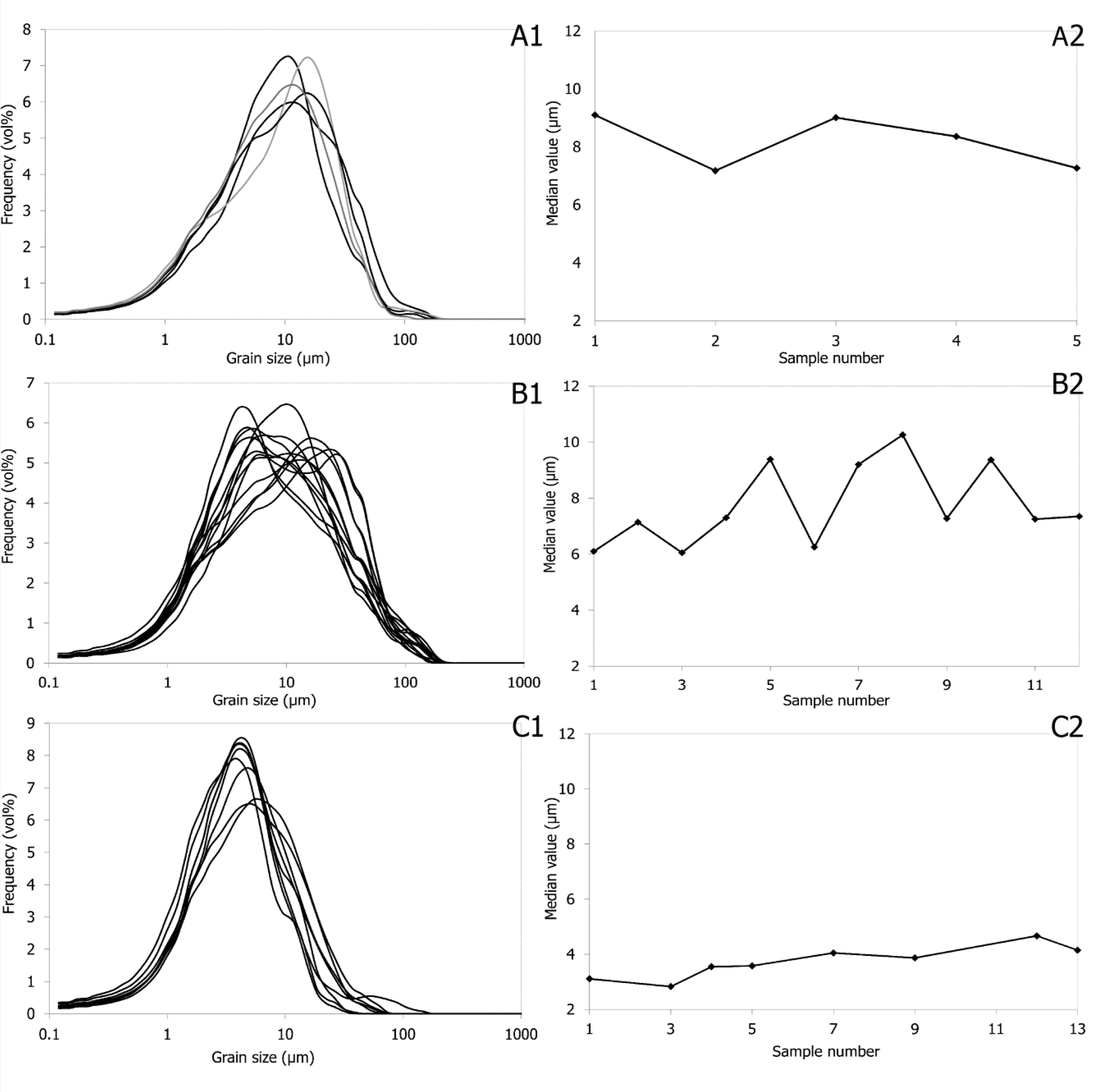
The field campaign included surface color analysis and sampling. Surface color analysis included the four documented types of surface materials based on false-color composite map (Figure 5). The colours of different surface deposits were determined using Munsell colours chart in the field: A is from 2.5 YR 8/2 to 5 YR 8/2 (light pink); B is from 2.5 YR 8/4 to 5 YR 8/4 (pink); C is 7.5 YR 6/3 to 7.5 YR 5/6 (light/strong brown). The samples were then analysed in terms of grain size with a Sympatec HELOS KR laser-diffraction particle sizer with a size range from 0.1–2000 µm. The results of the grain size analysis of field samples were used to validate the analysis of the false-color composite Landsat images on 11 November 2012 (Figure 6).We assigned the following names to the classes: A, salty surface; B, silt-rich surface; C, clay-rich surface; D, salt. Here, salty surface represents mixed sediments of salt and silt or clay with a light pink colour, while the silt-rich surface is coarser than the clay-rich surface. Salt indicated a thick, white salt crust on the surface.
With GPS data of the sampling sites, we collected training pixels of different surface materials on the Landsat image of 11 November 2012. Field observation showed that the surface was flat and homogeneous around each sample point. Therefore, we added training pixels around the sampling sites. We split the spectral datasets randomly into two sets: one set for training samples (Table 2) and the other for ground truth accuracy assessment. The training samples were analysed in terms of separability between classes with transformed divergence method [39].
4.3 Maximum Likelihood Classification
Evans [41] has proved that the prior knowledge of the relationships between input attributes and salinity in the classification of Landsat TM data is of importance for salinity mapping. We used a supervised classification, the MLC method, which employs discriminant functions to assign pixels to the class with the maximum likelihood [42].
4.4 Accuracy Assessment
The classification results were evaluated by different metrics including the overall accuracy, kappa coefficient, producer’s accuracy and user’s accuracy (Table 4). Due to the limited number of ground samples, the cross validation approach was implemented to make use of all the samples in both training the model and for the validation. The average of different runs was then used as the ultimate measure of the classification. The overall accuracy was 92.83% and the Kappa coefficient was 0.90.
4.5 Application to the Other Landsat Images Processing
The established spectral library based on the analysis of Landsat scene of 11 November 2012 was applied to other Landsat scenes for the period 1985–2011. We expanded the spectral libraries and randomly selected more than 1000 pixels with more than 10 polygons to training samples based on the classified map on 11 November 2012 (Figure 7). We used the toolbox “Endmember Collection” to perform classification on Landsat images from 1985–2011 with the remote sensing image processing software ENVI.
5. Results
5.1 Areal Statistical Analysis of the Different Classes
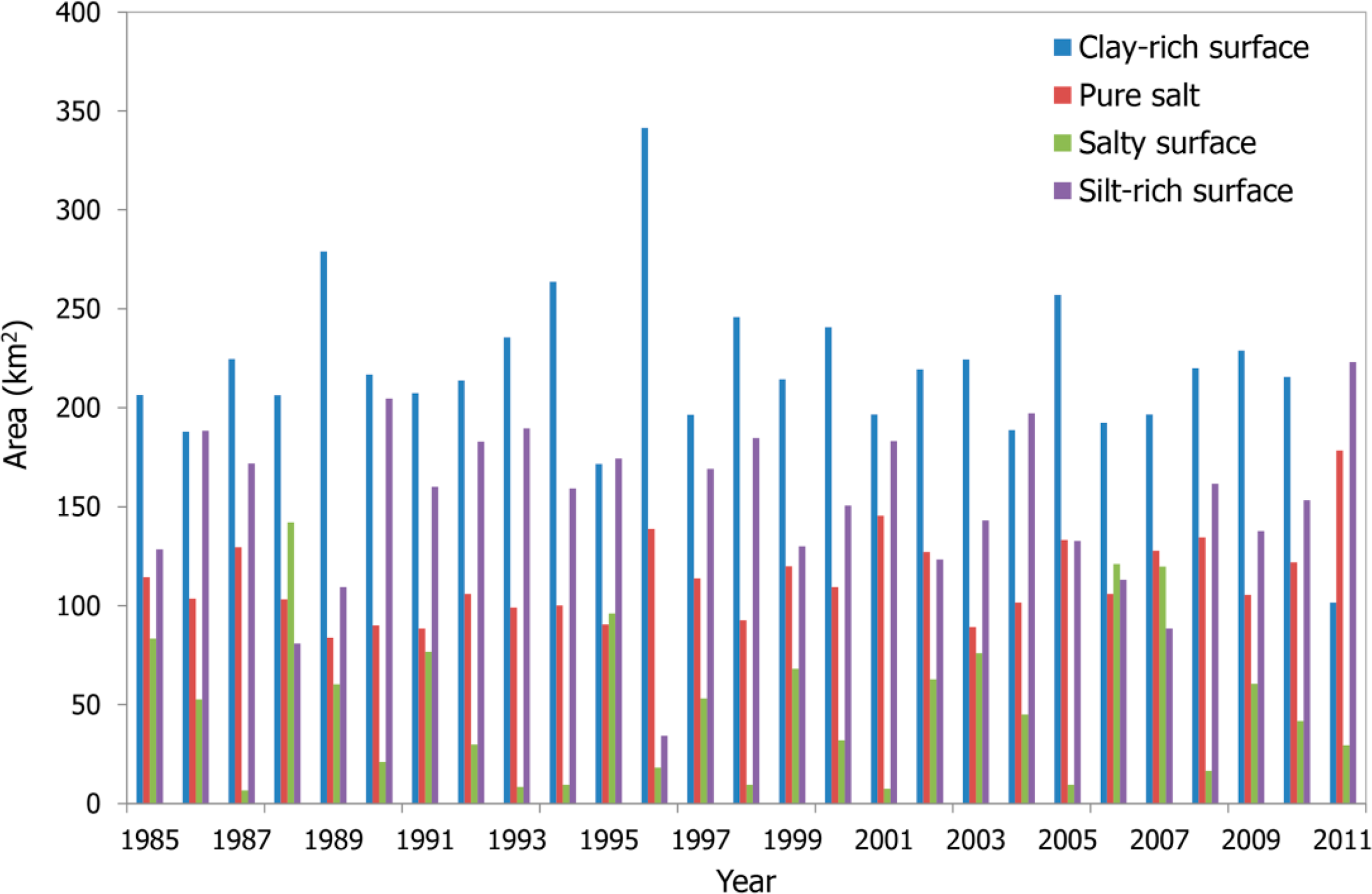
Surface materials change over years in terms of the area that they cover (Figure 8). The clay-rich surface is the most dominated surface material with a few exceptions over the period 1985–2011 (Table 5) covering on average 40% of the study area. According to the standard deviations, the salt remained consistent over time (with standard deviation of 21.48 km2) compared to the other surface materials in the study area. However, in the river terminus, all the three surfaces are characterized with large variations over time with standard deviations of 38.37 km2, 41.96 km2 and 41.27 km2 for salty, silt-rich and clay-rich surfaces, respectively. However, the classification results of the year 1996 showed very large discrepancies compared to the other years for the three surfaces which seemed to be abnormal in this case. We could not identify any specific reason for this discrepancy.
5.2 Interpretation of the Different Classes
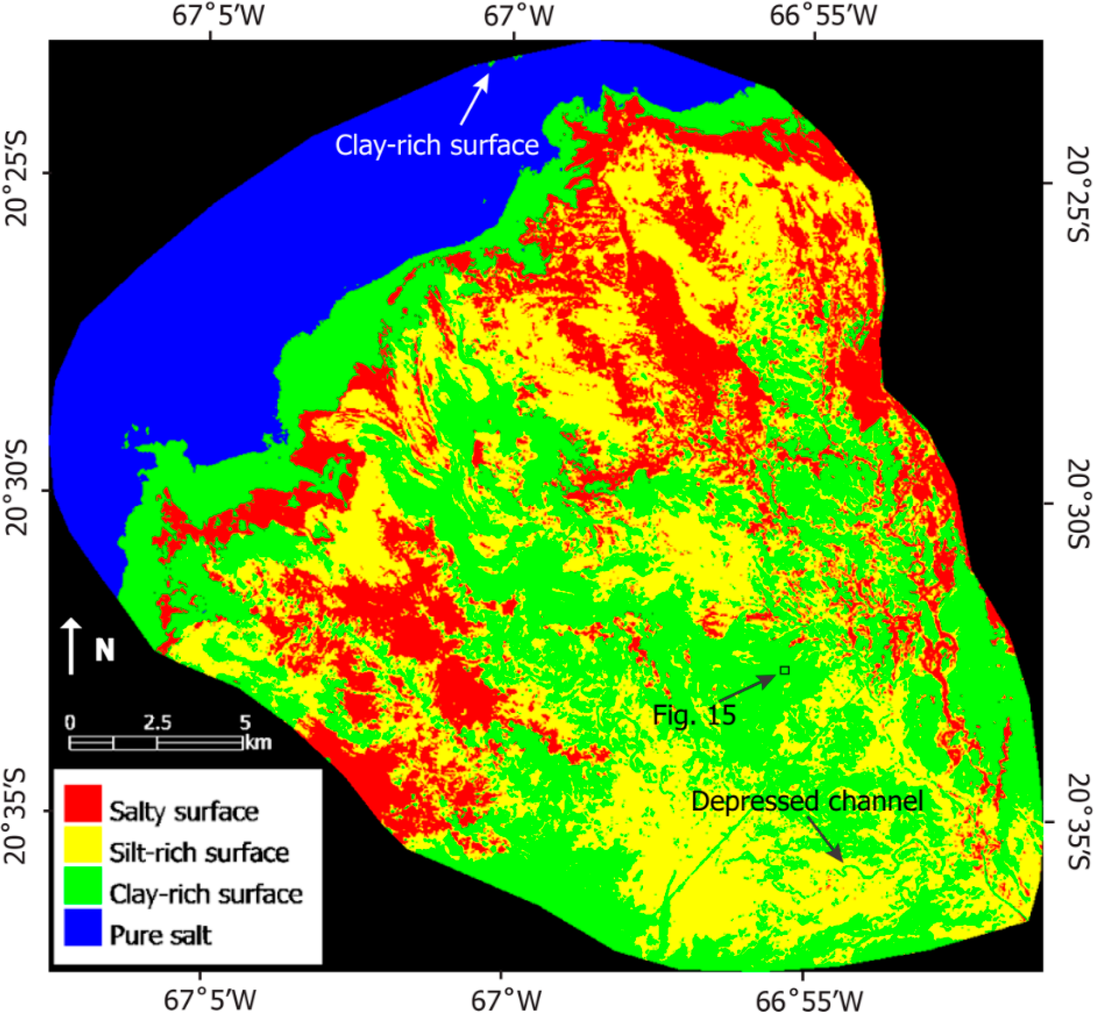
In the river terminus, the silt-rich surface and the clay-rich surface tend to be associated with different sedimentary facies. For example, the silt-rich surface is distributed on crevasse splays and levees along channels, while the clay-rich surface can be found on the floodplain between channels. In addition, the silt-rich surface was generally distributed in the proximal part of the river terminus while the clay-rich surface was commonly seen in the distal part of the terminus. The clay-rich surface sometimes could be seen in the salt lake, probably attributed to peak floods or wind (Figure 9). During peak floods, the water is at its highest level in the salt lake and clay is transported to the salt lake and the edge of the water body. When the water evaporates and salt is precipitated, the clay in the deep water area is covered by salt but clay at the edge of the water body is mixed with salt and exposed. Depressed channels were also covered by the clay-rich surface, although sometimes salt could be found in the present channel (Figure 9). The salty surface was generally distributed in the channels and the distal part of the river terminus, while the salt was generally distributed at the end of the present channel and the salt lake.
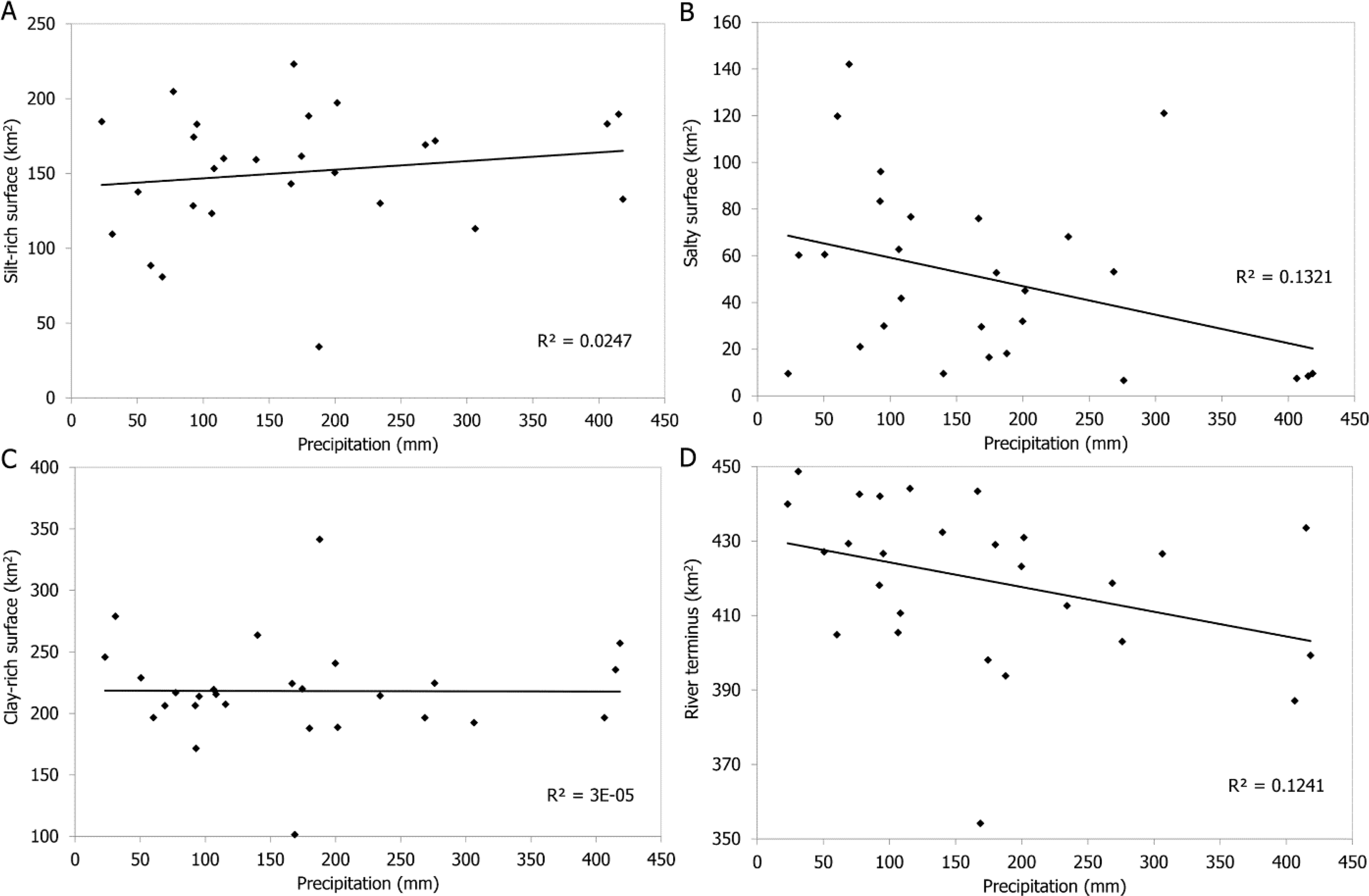
In combination with the annual precipitation, we analysed the areal changes of each class between 1985 and 2011. The silt-rich surface shows a weak correlation with the annual precipitation (Figure 10A) probably because although the annual precipitation is high, the daily precipitation all year around is low. However, some daily precipitation is high in those low annual precipitation periods and Li et al. [21] have demonstrated that high daily precipitation would lead to peak discharges, which result in large flow and sediments transport to the river terminus. During these short-lived and high magnitude of peak floods or multiple successive floods, channels experience massive over-spilling flow due to the downstream decrease in cross-section area on the low-gradient Río Colorado river system [21,43] and the spill-over flow reactivates crevasse splays and levees. For instance, the crevasse splay was partly reactivated in the rainy season of 1999–2000. However, it was completely reactivated in the rainy season of 2000–2001 because of the highest annual precipitation (406.4 mm) in the period from 1985 to 2011 (Figure 11).
By contrast, the salty surface was negatively correlated with the annual precipitation (Figure 10B), i.e., when the annual precipitation increased, the salty surface decreased. For the clay-rich surface, there is no correlation with the annual precipitation (Figure 10C). The area of river terminus, which includes salty surface, silt- and clay-prone surface, tended to be inversely proportional to the annual rainfall (Figure 10D). This is likely due to the fact that the higher the annual rainfall, the more water is draining to the lake, which results in high water levels in the lake. When the water evaporates, salt is precipitated on the surface. Therefore, the salt area will increase and the river terminus shrinks when the annual precipitation increases.
5.3 Geomorphological Change Detection
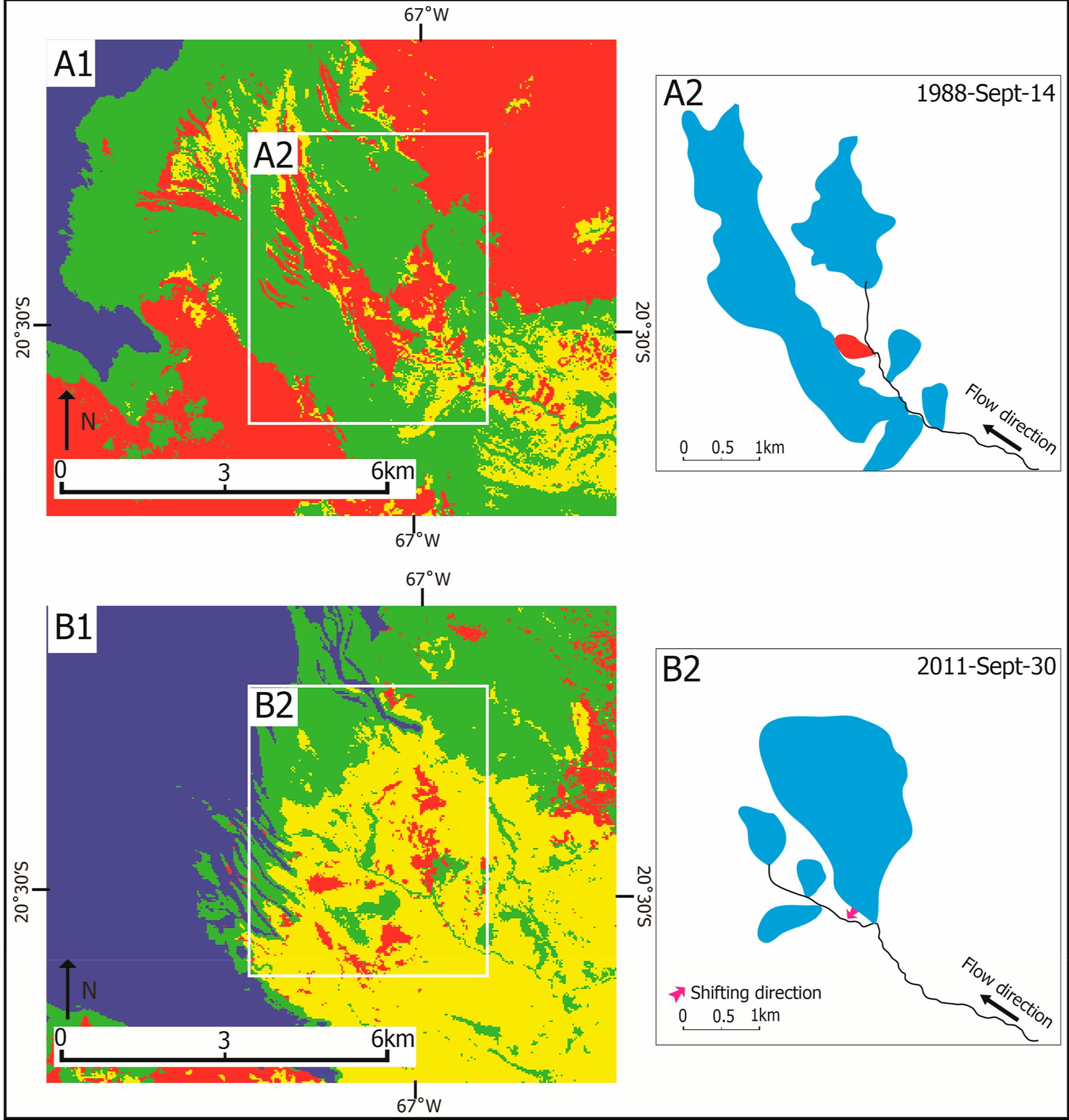
Geomorphological changes can be visualized with comparisons of classification maps. The positive correlation between silt-rich surface and crevasse splays enables us to characterise the expansion of crevasse splays over the observation years. Specifically, the development of a crevasse splay in the distal part of the river terminus was recorded through time-series classification maps. It started with a small crevasse splay and then grew into large splays during the subsequent floods (Figure 12). The expansion of the crevasse splay is in agreement with that by Li et al. [21], which also showed that this new crevasse splay was attributed to a compensational stacking pattern, whereby the new crevasse splay expanded in the topographic low between two adjacent existing splays. The expansion of crevasse splays also contributed to the increasing area of the silt-rich surface.
The avulsion history was reconstructed by comparing classification maps (Figure 13). The observed avulsion was initiated with a crevasse splay and then developed into an avulsion with subsequent floods. Previous studies suggested that the splay-induced avulsions are attributed to downstream decrease in channel cross-section area in the dryland river system [21,43]. Therefore, rivers in the low-gradient dryland region experience massive flow over-spilling onto the floodplain, which reinforces levee breaches during peak floods, and increases the chance of bank failure. In addition, the sediment-laden water would flow back to the trunk channel during the waning flood stage. The returning flow erodes the crevasse floor and deepens the crevasse channels; on the other hand, the process decreases the capacity of the trunk channel because sediments in the returning flow are deposited at the downstream side due to low energy of returning flow [43]. These processes promote avulsions and simultaneously increase the silt-rich surface in the distal part of the river terminus.
6. Discussion
Due to salinity, the Time Domain Reflectometry (TDR), which is used to simultaneously obtain soil water content and electrical conductivity by a single probe with a minimal disturbance [44], did not work properly. However, field observation showed that the clay-rich surface is wetter than the silt-rich surface (Figure 14A). In addition, the density of desiccation cracks (Figure 14B) is also higher on the clay-rich surface than on the silt-rich surface. Both soil moisture and desiccation cracks exert a reduction on reflectance.
In order to check the consistency of the surface reflectance for different years over the study area, we selected an area of 70 pixels located in the centre of a clay-rich surface on both 11 November 2012 and 30 September 2011 images (Figure 15). The tested area is in the centre of a floodplain area (Figure 9) which is marginally influenced by peak discharge. As seen in the figure, the extracted reflectances show good agreement between the two dates. However, some differences are still seen between the two images, partly due to the differences in the sensor configurations and partly due to the pre-processing of the images or changes in the area over time. In general, the absolute difference between the two reflectances is mostly lower than 3% (reflectance), which can be considered as a reasonable threshold for classification.
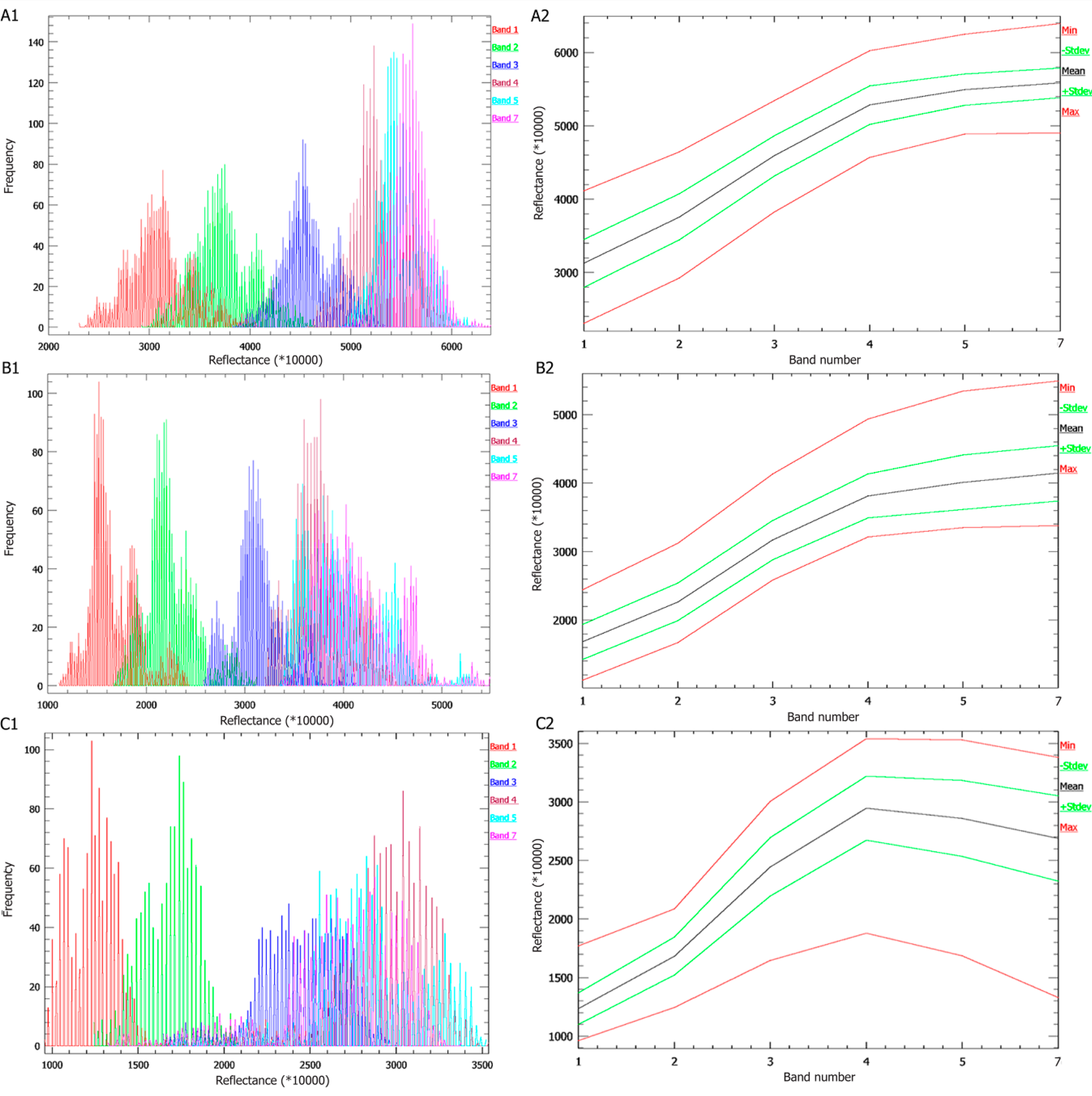
By comparing the reflectance of different classes (see Figure 7), it can be seen that the mean values are very different for each class, though they show similar trends. This might lead to the conclusion that classification methods based on angular mapping would work better in such a case. In order to demonstrate this, we have implemented other classification methods based on angular mapping like Spectral Angle Mapper (SAM) and as well as Support Vector Machine (SVM). However, these two methods showed lower accuracies (not shown) compared to the maximum likelihood method and failed in producing reasonable classification maps. Moreover, the classification results show the tested area is classified the same (i.e., silt-rich surface) in the two images using maximum likelihood method demonstrating that the good performance of the method.
We also suggest that post-processing such as majority/minority analysis, sieve classes should not be performed on classification maps. First of all, the inter-channel deposits are generally clay-rich and, therefore, their reflectance is low. In addition, the inter-channel area is sometimes small (e.g., crevasse channels) with the ground resolution of the Landsat TM images being 30 m by 30 m. Using these post-processing methods tends to blur these sedimentary phenomena and create errors. Therefore, the statistical analysis on playa morphodynamics was found the result of maximum likelihood classification to be better than that with post-processing.
Surface reflectance from false-color composite images was used to differentiate surface materials, and these surface materials correspond to a particular color (Figure 5), but still with some errors. For example, some sampling locations apparently look pink and samples from these places are supposed to be silt-rich, but the grain size analysis shows that these samples belong to clay-rich materials.
7. Conclusions
This paper contributes to the understanding of playa surface dynamics using remotely sensed data over a period of 27 years, from 1985–2011. The study investigates potentials of multi-temporal Landsat surface reflectance in mapping coarse and fine sediments in the river terminus of the Salar de Uyuni, Bolivia. First, spectral libraries were generated based on the Landsat surface reflectance image of 2012 and field data analysis corresponding to the ground truth data for four different surface materials in the river terminus. These surface materials were salty, silt-rich, clay-rich and salt surface. Such spectral libraries were then used to classify the Landsat image using Maximum likelihood method. The cross validation approach was implemented to validate the classified map. The overall accuracy of 92.83% and the Kappa coefficient of 0.90 were achieved. Second, the consistency of the reflectance over time for different images was investigated. For instance, the absolute difference between reflectances of the images of 2011 and 2012 were found to be mostly lower than 3% (reflectance) which was considered as a reasonable threshold for classification. Finally, the spectral libraries were used to classify the other Landsat images from different years over the study area.
According to the classified maps, the clay-rich surface remained the most dominant surface material with a few exceptions over the entire period covering approximately on average 40% of the study area. The salt was relatively stable in terms of area over time (with standard deviation of 21.48 km2) compared to the other surface materials in the study area. However, in the river terminus, all the three surfaces are characterized with large variations over time with standard deviations of 38.37 km2, 41.96 km2 and 41.27 km2 for salty, silt-rich and clay-rich surfaces, respectively. The silt-rich surface and the clay-rich surface are associated with different sedimentary facies in the river terminus. The silt-rich surface was widely distributed along channels and crevasse splays while the clay-rich surface was found in the floodplain and the channels. In addition, the proximal part of the river terminus was dominated by the silt-rich surface while the distal part of the terminus was mainly occupied by the clay-rich surface. The clay-rich surface occurs in the salt lake during floods or through wind-blown influence. The silt-rich surface has a weak correlation with the annual precipitation while the salty surface tends to be inversely proportional to the annual precipitation. High annual precipitations have better chances to reactivate rivers in the playa and lead to over-spilling flows onto levees and crevasse splays due to downstream decrease in bankfull width and depth. Geomorphological changes have been identified such as the formation of crevasse splays and avulsions. High annual precipitation-induced avulsions also led to increased silt-rich surfaces.
Acknowledgments
Jiaguang Li would like to thank the fieldwork sponsors including the Molengraaff Fund and the International Association of Sedimentologists. Jiaguang Li also thanks Seyed Enayat Hosseini Aria for the fruitful discussion in the beginning of the work. The comments and suggestions of the anonymous reviewers are also very much appreciated.
Author Contributions
Jiaguang Li led the research work, proposed the idea and conducted the research work including field sampling and laboratory analysis, as well as well finished the manuscript. Massimo Menenti, Alijafar Mousivand and Stefan M. Luthi deeply contributed to improving the quality of this manuscript.
Conflicts of Interest
The authors declare no conflict of interest.
References
- Castañeda, C.; Herrero, J.; Casterad, M.A. Landsat monitoring of playa-lakes in the Spanish Monegros desert. J. Arid Environ 2005, 63, 497–516. [Google Scholar]
- Bryant, R.G. Validated linear mixture modelling of Landsat TM data for mapping evaporate minerals on a playa surface. Int. J. Remote Sens 1996, 17, 315–330. [Google Scholar]
- McKie, T. A comparison of modern dryland depositional systems with the Rotliegend Group in The Netherlands. In The Permian Rotliegend in The Netherlands; Grotsch, J., Gaupp, R., Eds.; SEPM: Tulsa, OK, USA, 2011; Volume 98, pp. 89–103. [Google Scholar]
- Hardie, L.A.; Smoot, J.P.; Eugster, H.P. Saline lakes and their deposits: A sedimentological approach. In Modern and Ancient Lake Sediments; Mater, A., Tucker, M.E., Eds.; SEPM: Tulsa, OK, USA, 1978; pp. 7–41. [Google Scholar]
- Rosen, M.R. Sedimentologic and geochemical constraints on the evolution of Bristol Dry Lake Basin, California, U.S.A. Palaeogeogr. Palaeoclimatol. Palaeoecol 1991, 84, 229–257. [Google Scholar]
- Bryant, R.G. The Sedimentology Geochemistry of Non-Marine Evaporates on the Chott el Djerid Using both Ground and Remotely Sensed Data. Ph.D Thesis. University of Reading, Reading, UK, 1993. [Google Scholar]
- Bryant, R.G.; Drake, N.A.; Millington, A.C.; Sellwood, B.W. The chemical evolution of the brines of Chott el Dijerid, Southern Tunisia, after an exceptional rainfall event in January 1990. In The Sedimentology and Geochemistry of Modern and Ancient Saline Lakes; Renaut, R.W., Last, W.M., Eds.; SEPM: Tulsa, OK, USA, 1994; pp. 3–12. [Google Scholar]
- Menenti, M.; Lorkeers, A.; Vissers, M. An application of thematic mapper data in Tunesia. ITC J 1986, 1, 35–42. [Google Scholar]
- Menenti, M.; Bastiaanssen, W.G.M.; van Eick, D. Determination of hemispheric reflectance with Thematic Mapper data. Remote Sens. Environ 1989, 28, 327–337. [Google Scholar]
- Townshend, J.R.G.; Quarmby, N.A.; Millington, A.C.; Drake, N.A.; White, K.H. Monitoring playa sediment transport systems using Thematic Mapper data. Adv. Space Res 1989, 9, 177–183. [Google Scholar]
- Drake, N.A.; Bryant, R.G.; Millington, A.C.; Townshend, J.R.G. Playa sedimentology and geomorphology: Mixture modelling applied to Landsat Thematic Mapper data of Chott el Djerid, Tunisia. In The Sedimentology and Geochemistry of Modern and Ancient Saline Lakes; Renaut, R.W., Last, W.M., Eds.; SEPM: Tulsa, OK, USA, 1994; pp. 32–42. [Google Scholar]
- Drake, N.A. Reflectance spectra of evaporite minerals (400–2500nm): Applications for remote sensing. Int. J. Remote Sens 1995, 16, 2555–2571. [Google Scholar]
- Bryant, R.G. Monitoring climatically sensitive playas using AVHRR data. Earth Surf. Proc. Land 1999, 24, 283–302. [Google Scholar]
- Bryant, R.G.; Rainey, M.P. Investigation of flood inundation on playas within the Zone of Chotts, using a time-series of AVHRR. Remote Sens. Environ 2002, 82, 360–375. [Google Scholar]
- Ghrefat, H.A.; Goodell, P.C. Land cover mapping at Alkali Flat and Lake Lucero, White Sands, New Mexico, USA using multi-temporal and multi-spectral remote sensing data. Int. J. Appl. Earth Obs. Geoinf 2011, 13, 616–625. [Google Scholar]
- Chapman, J.E.; Rothery, D.A.; Francis, P.W.; Pontual, A. Remote sensing of evaporate mineral zonation in salt flats (salars). Int. J. Remote Sens 1989, 10, 245–255. [Google Scholar]
- Johnston, R.; Kamprad, J. Application of Landsat Thematic Mapper to geology and salinity in the Murray Basin. BMR J. Aust. Geol. Geophys 1989, 11, 363–366. [Google Scholar]
- Millington, A.C.; Drake, N.A.; Townshend, J.R.G.; Quarmby, N.A.; Settle, J.J.; Reading, A.J. Monitoring salt playa dynamics using Thematic Mapper data. IEEE Trans. Geosci. Remote Sens 1989, 27, 754–761. [Google Scholar]
- Quarmby, N.A.; Townshend, J.R.G.; Millington, A.C.; White, K.H.; Reading, A.J. Monitoring sediment transport systems in a semi-arid area using Thematic Mapper data. Remote Sens. Environ 1989, 28, 305–315. [Google Scholar]
- Rainey, M.P.; Tyler, A.N.; Gilvear, D.J.; Bryant, R.G.; McDonald, P. Mapping intertidal estuarine sediment grain size distributions through airborne remote sensing. Remote Sens. Environ 2003, 86, 480–490. [Google Scholar]
- Li, J.; Donselaar, M.E.; Hosseini Aria, S.E.; Koenders, R.; Oyen, A.M. Landsat imagery-based visualization of the geomorphological development at the terminus of a dryland river system. Quat. Int 2014, 7. [Google Scholar] [CrossRef]
- Hilhorst, M.A.; Dirksen, C.; Kampers, F.W.H.; Feddes, R.A. Dielectric relaxation of bound water versus soil matric pressure. Soil Sci. Soc. Am. J 2001, 65, 311–314. [Google Scholar]
- Dewey, J.F.; Bird, J.M. Mountain belts and the new global tectonics. J. Geophys. Res 1970, 75, 2625–2647. [Google Scholar]
- Horton, B.K.; DeCelles, P.G. Modern and ancient fluvial megafans in the foreland basin system of the central Andes, southern Bolivia: Implications for drainage network evolution in fold-thrust belts. Basin Res 2001, 13, 43–63. [Google Scholar]
- Isacks, B.L. Uplift of the central Andean plateau and bending of the Bolivian orocline. J. Geophys. Res 1988, 93, 3211–3231. [Google Scholar]
- Jordan, T.E.; Reynolds, J.H.; Erikson, J.P. Variability in age of initial shortening and uplift in the central Andes, 16–33°30′S. In Tectonic Uplift and Climate Change; Ruddiman, W.F., Ed.; Plenum Press: New York, NY, USA, 1997; pp. 41–61. [Google Scholar]
- Horton, B.K.; Hampton, B.A.; Waanders, G.L. Paleogene synorogenic sedimentation in the Altiplano plateau and implications for initial mountain building in the central Andes. Geol. Soc. Am. Bull 2001, 113, 1387–1400. [Google Scholar]
- Elger, K.; Oncken, O.; Glodny, J. Plateau-style accumulation of deformation: Southern Altiplano. Tectonics 2005, 24. [Google Scholar] [CrossRef]
- Placzek, C.J.; Quade, J.; Patchett, P.J. A 130 ka reconstruction of rainfall on the Bolivian Altiplano. Earth Planet. Sci. Lett 2013, 363, 97–108. [Google Scholar]
- Argollo, J.; Mourguiart, P. Late Quaternary climate history of the Bolivian Altiplano. Quat. Int 2000, 72, 37–51. [Google Scholar]
- Grosjean, M. Paleohydrology of the Laguna Lejia (north Chilean Altiplano) and climactic implications for late-glacial times. Palaeogeogr. Palaeoclimatol. Palaeoecol 1994, 109, 89–100. [Google Scholar]
- Risacher, F.; Fritz, B. Origin of salts and brine evolution of Bolivian and Chilean salars. Aquat. Geochem 2009, 15, 123–157. [Google Scholar]
- Lenters, J.D.; Cook, K.H. Summertime precipitation variability over South America: Role of the Large-Scale circulation. Mon. Weather Rev 1999, 127, 409–431. [Google Scholar]
- Yuan, F.; Sawaya, K.E.; Loeffelholz, B.C.; Bauer, M.E. Land cover mapping and change analysis in the Twin Cities Metropolitan Area with Landsat remote sensing. Remote Sens. Environ 2005, 98, 317–328. [Google Scholar]
- Stefanov, W.L.; Ramsey, M.S.; Christensen, P.R. Monitoring urban land cover change: An expert system approach to land cover classification of semiarid to arid urban centers. Remote Sens. Environ 2001, 77, 173–185. [Google Scholar]
- Foody, G.M.; Ghoneim, E.M.; Arnell, N.W. Predicting locations sensitive to flash flooding in an arid environment. J. Hydrol 2004, 292, 48–58. [Google Scholar]
- Elnaggar, A.A.; Noller, J.S. Application of remote-sensing data and decision-tree analysis to mapping salt-affected soils over large areas. Remote Sens 2010, 2, 151–165. [Google Scholar]
- Canty, M.J.; Nielsen, A.A. Automatic radiometric normalization of multitemporal satellite imagery with the iteratively re-weighted MAD transformation. Remote Sens. Environ 2008, 112, 1025–1036. [Google Scholar]
- Swain, P.H.; King, R.C. Two effective feature selection criteria for multispectral remote sensing. Proceedings of the First International Joint Conference on Pattern Recognition, Washington DC, USA, 30 October–1 November 1973; pp. 536–540.
- Petropoulos, G.P.; Vadrevu, K.P.; Xanthopoulos, G.; Karantounias, G.; Scholze, M. A comparison of spectral angle mapper and artificial neural network classifiers combined with Landsat TM imagery analysis for obtaining burnt area mapping. Sensors 2010, 10, 1967–1985. [Google Scholar]
- Evans, F. An investigation into the use of maximum likelihood classifiers, decision trees, neural networks and conditional probabilistic networks for mapping and predicting salinity. Master’s Thesis, School of Computer Science. Curtin University of Technology, Perth, WA, Australia, 1998. [Google Scholar]
- Strahler, A.H. The use of prior probabilities in maximum likelihood classification of remotely sensed data. Remote Sens. Environ 1980, 10, 135–163. [Google Scholar]
- Donselaar, M.E.; Cuevas Gozalo, M.C.; Moyano, S. Avulsion processes at the terminus of low-gradient semi-arid fluvial systems: Lessons from the Río Colorado, Altiplano endorheic basin, Bolivia. Sediment. Geol 2013, 283, 1–14. [Google Scholar]
- Noborio, K. Measurement of soil water content and electrical conductivity by time domain reflectometry: A review. Comput. Electron. Agric 2001, 31, 213–237. [Google Scholar]


| Day | Month | Year | Day | Month | Year |
|---|---|---|---|---|---|
| 5 | August | 1985 | 16 | November | 1999 |
| 11 | October | 1986 | 2 | November | 2000 |
| 23 | November | 1987 | 21 | November | 2001 |
| 14 | September | 1988 | 25 | June | 2002 |
| 4 | November | 1989 | 26 | October | 2003 |
| 7 | November | 1990 | 13 | November | 2004 |
| 9 | October | 1991 | 31 | October | 2005 |
| 9 | September | 1992 | 19 | November | 2006 |
| 26 | July | 1993 | 5 | October | 2007 |
| 27 | June | 1994 | 8 | November | 2008 |
| 20 | October | 1995 | 26 | October | 2009 |
| 20 | September | 1996 | 26 | August | 2010 |
| 6 | August | 1997 | 30 | September | 2011 |
| 10 | September | 1998 | 11 | November | 2012 |
| Class | Pixels | Polygons |
|---|---|---|
| Salty surface | 34 | 3 |
| Silt-rich surface | 41 | 6 |
| Clay-rich surface | 60 | 5 |
| Pure salt | 41 | 8 |
| Class-1 | Class-2 | Separability |
|---|---|---|
| Salty surface | Silt-rich surface | 1.998 |
| Salty surface | Clay-rich surface | 2.000 |
| Salty surface | Pure salt | 2.000 |
| Silt-rich surface | Clay-rich surface | 1.980 |
| Silt-rich surface | Pure salt | 2.000 |
| Clay-rich surface | Pure salt | 2.000 |
| Class | Producer’s Accuracy (%) | User’s Accuracy (%) |
|---|---|---|
| Salty surface | 92.5 | 95 |
| Silt-rich surface | 91.96 | 88.48 |
| Clay-rich surface | 91.87 | 92.42 |
| Pure salt | 92.33 | 100 |
| Class | Mean (km2) | Max (km2) | Min (km2) | Standard Deviation (km2) |
|---|---|---|---|---|
| Salty surface | 50.28 | 142.07 | 6.61 | 38.37 |
| Silt-rich surface | 150.92 | 223.09 | 34.22 | 41.96 |
| Clay-rich surface | 218.27 | 341.44 | 101.56 | 41.27 |
| Salt | 113.09 | 178.36 | 83.86 | 21.48 |
© 2014 by the authors; licensee MDPI, Basel, Switzerland This article is an open access article distributed under the terms and conditions of the Creative Commons Attribution license (http://creativecommons.org/licenses/by/4.0/).
Share and Cite
Li, J.; Menenti, M.; Mousivand, A.; Luthi, S.M. Non-Vegetated Playa Morphodynamics Using Multi-Temporal Landsat Imagery in a Semi-Arid Endorheic Basin: Salar de Uyuni, Bolivia. Remote Sens. 2014, 6, 10131-10151. https://doi.org/10.3390/rs61010131
Li J, Menenti M, Mousivand A, Luthi SM. Non-Vegetated Playa Morphodynamics Using Multi-Temporal Landsat Imagery in a Semi-Arid Endorheic Basin: Salar de Uyuni, Bolivia. Remote Sensing. 2014; 6(10):10131-10151. https://doi.org/10.3390/rs61010131
Chicago/Turabian StyleLi, Jiaguang, Massimo Menenti, Alijafar Mousivand, and Stefan M. Luthi. 2014. "Non-Vegetated Playa Morphodynamics Using Multi-Temporal Landsat Imagery in a Semi-Arid Endorheic Basin: Salar de Uyuni, Bolivia" Remote Sensing 6, no. 10: 10131-10151. https://doi.org/10.3390/rs61010131
APA StyleLi, J., Menenti, M., Mousivand, A., & Luthi, S. M. (2014). Non-Vegetated Playa Morphodynamics Using Multi-Temporal Landsat Imagery in a Semi-Arid Endorheic Basin: Salar de Uyuni, Bolivia. Remote Sensing, 6(10), 10131-10151. https://doi.org/10.3390/rs61010131