Characterizing Rainfall Discrepancies Between Landslide Sites and the Nearest Rain Gauges Using Radar Estimates: A Case Study from Italy

Highlights

What are the main findings?

• Analysis of 548 rainfall events triggering landslides in Italy, using 1 km² radar rainfall estimates, reveals potentially significant discrepancies between rainfall at landslide locations and at the nearest rain gauge.
• The probability of large rainfall discrepancies increases with gauge–landslide distance, but substantial differences may occur even at short distances, particularly during convective (summer) events.

What are the implications of the main findings?

• Rain gauge-based estimates of landslide-triggering rainfall may involve substantial uncertainty due to the spatial variability of precipitation.
• High-resolution distributed radar rainfall products can improve the reconstruction of triggering rainfall and support more reliable rainfall thresholds.

Abstract

The spatial representativeness of rain gauges is critical for accurately estimating rainfall that triggers landslides and for defining operational thresholds. This study evaluates the potential error in conventional rain-gauge-based methods for estimating landslide-triggering rainfall, using 548 landslide events across Italy from the e-ITALICA database, which reports the duration of each rainfall event and the location of the nearest available rain gauge. A radar-based assessment, using the Surface Rainfall Intensity (SRI) product (1 km² resolution) provided by the Italian Department of Civil Protection, quantified discrepancies between rainfall at landslide locations and at the nearest rain gauges. Seasonal analysis was performed, considering summer events (April–September), typically associated with convective and spatially variable rainfall, and winter events (October–March), generally more stratiform and uniform rainfall. Results indicate that the probability of large discrepancies increases with distance. Summer events show larger discrepancies at short distances compared to winter events, but seasonal distributions converge at larger distances. These findings provide useful insights into rain gauge representativeness in studies of rainfall-induced landslides.

1. Introduction

Landslides represent one of the major natural hazards worldwide, causing significant human and economic losses. Landslides affect ecosystems, causing biodiversity loss, soil alteration, and environmental degradation. They also produce direct impacts in human-impacted areas, such as fatalities and destruction of buildings and infrastructure, and indirect impacts, including service disruption, productivity loss, and long-term economic costs [1]. Globally, tens of thousands of fatalities are reported each year due to landslide events [2,3], with substantial economic losses estimated in the tens of billions of USD annually [4,5]. Italy is among the most affected European countries, with high annual losses and a considerable number of fatalities [4,5,6,7,8]. Given their substantial environmental, human, and economic impacts, landslide risk therefore represents a critical issue that must be systematically addressed in both research and risk management frameworks, attracting widespread attention from the academic community [9]. Moreover, since landslides are complex phenomena influenced not only by geological and meteorological factors but also by social and economic dynamics, their study requires a multidisciplinary approach [10].

Although landslides can be triggered by earthquakes, volcanic eruptions, or human activities, intense and/or prolonged rainfall remains the dominant factor worldwide [1,2,5,7,11]. The documented increase in extreme precipitation, likely linked to climate change, contributes to a rise in rainfall-induced landslides, increasing the risks for populations living in vulnerable areas [5,10,11,12,13,14].

For accurate characterization of rainfall-induced landslides, assessing the rainfall conditions responsible for initiation is essential. While physically based approaches considering both rainfall and site predisposition would be ideal, they are often impractical over large areas. Consequently, statistical analyses of historical rainfall events are widely adopted, with empirical rainfall thresholds, such as intensity–duration (I–D) or event rainfall–duration (E–D) relationships, commonly used to identify triggering conditions [15,16,17]. Accurate reconstruction of rainfall distribution is therefore essential for reliably assessing landslide hazard and for implementing effective risk assessment and mitigation strategies within Decision Support Systems (DSSs) and early warning systems.

Precipitation is traditionally measured using ground-based rain gauge networks, which provide accurate and high-temporal-resolution data. However, gauges measure precipitation at single points, while rainfall is spatially distributed and structured across multiple scales. Reconstructing rainfall fields from point data is therefore challenging and highly dependent on network density and distribution [18]. Hydrological processes occur across a wide range of spatial and temporal scales, from millimeters to thousands of kilometers and from seconds to decades. The term ‘scale’ refers to the characteristic spatial or temporal extent of a process, or the resolution at which it is best observed. Many studies have classified these scales, focusing particularly on interactions between rainfall and other hydrological processes. Early work [19] introduced a logarithmic framework to represent spatial and temporal variability, which was later expanded by other authors to include urban processes, floods, and droughts. Even dense networks can fail to capture local precipitation maxima, thereby underestimating intense events that often trigger landslides [20,21], especially localized convective events in small catchments [22]. This limitation is likely to become more critical under climate change, which increases the frequency and intensity of extreme convective rainfall [23], and is further exacerbated in mountainous areas, where station density is limited despite higher landslide susceptibility [24].

Uncertainty related to the spatial and temporal variability of rainfall is a major source of error in estimating hydrological response. Many studies have addressed rain gauge errors, rainfall uncertainty, and their impact on rainfall thresholds [25,26,27]. For example, [27] demonstrates that rainfall uncertainty propagates into threshold curves, while [25] shows that thresholds derived from different data sources shift systematically (e.g., satellite vs. gauge). Similarly, [26] identifies rain gauge inaccuracies, timing errors, and poor spatial representativeness as major sources of threshold uncertainty.

New technologies have improved the accuracy and resolution of rainfall measurements. While rain gauges remain the most widely used instruments, weather radars provide high-resolution data, but need to be combined with gauge networks to ensure reliable estimates [28]. Quantitative Precipitation Estimates (QPEs) derived from remote sensing technologies, such as weather radar and satellites [29,30], provide spatially distributed rainfall data. These products play a key role in overcoming the limited spatial coverage of rain gauge networks and better capturing rainfall patterns that trigger landslides. Satellite-based QPEs, for example, allow near real-time monitoring of large areas and can generally identify rainfall events that trigger landslides, which is particularly useful in regions with sparse rain gauge networks [25,31]. However, their performance varies across different satellite products and the areas in which these products are applied [32]. Moreover, the gridded nature of the data can smooth out local peaks, underestimating intense events and sometimes overestimating lighter rainfall, which affects early warning threshold estimates [33]. Careful consideration of spatial resolution is therefore essential when using satellite QPEs to assess landslide-triggering rainfall.

Radar data, which generally offer higher spatial resolution than satellite data, provide significant advantages by better capturing local precipitation peaks and triggering conditions. Several studies have shown that radar-derived rainfall fields improve the estimation of landslide initiation thresholds. For example, [34] used 5 × 5 km² radar data to derive rainfall thresholds for 75 rainfall-induced landslides in Scotland, showing improvements over the use of rain gauges alone. Radar allowed site-specific rain records that reduced uncertainties from distant gauges and better captured localized convective events, particularly in mountainous areas. As shown in [35] for a study in the Sichuan Basin (China), at finer 1 × 1 km² resolution, these benefits are further enhanced: rainfall spatial variability is more accurately characterized, predictive performance of initiation thresholds improves, false alarms are reduced, and the ability to distinguish triggering from non-triggering events is strengthened.

Similar results have been reported in Italy, where radar-based QPEs at 1 × 1 km² spatial resolution are operationally provided by the National Department of Civil Protection (DPC). Radar estimates, particularly when bias correction is applied using rain gauge observations, allow the definition of more accurate rainfall thresholds, for example, for debris-flow initiation [36]. Conversely, thresholds derived solely from gauges often underestimate localized maxima. Even without bias correction, radar-derived fields improve the identification of rainfall peaks at landslide locations, with important implications for estimating triggering rainfall compared to the nearest gauge, even in small areas with relatively dense rain gauge networks [20].

The fine spatial resolution of radar data is therefore crucial for accurately characterizing landslide-triggering rainfall, providing more reliable thresholds and reducing biases associated with the limited spatial representativeness of point measurements.

In the present study, the error associated with using the nearest available rain gauge to estimate rainfall triggering landslides was assessed by comparing rainfall at the gauge with that at the landslide site. Both quantities were derived from 1 km² radar products provided by the DPC. This approach relies on analyzing relative discrepancies between gauge and landslide rainfall, removing the need to calibrate radar data against point measurements. The analysis used a dataset of 548 landslides across Italy between 2010 and 2021, selected from the e-ITALICA database [37]. Discrepancies were examined with respect to the distance between gauge and landslide, and seasonal differences were also considered, distinguishing periods dominated by uniform stratiform precipitation from those with more localized convective events. The results highlight the limitations of relying solely on rain gauge measurements, showing how spatial variability in precipitation can affect the representativeness of point observations at the landslide site. The study also points to the potential of high-resolution radar products for a more accurate characterization of triggering conditions, which could enhance risk assessment and early warning systems.

2. Data

Italy is widely recognized as one of the European countries most exposed to landslide hazards, due to its complex geological and geomorphological setting. A large portion of the national territory is characterized by mountainous and hilly landscapes, combined with heterogeneous lithology, active tectonics, and significant climatic variability, all of which contribute to slope instability [38,39]. In addition, human activities such as urban expansion and land-use changes often exacerbate natural susceptibility. As a result, landslides represent one of the most frequent and damaging natural hazards in Italy, causing significant impacts on infrastructure, the economy, and population [39,40].

Within this framework, the datasets used in this study include a landslide inventory and radar-derived rainfall observations, which are described in the following sub-sections.

2.1. Landslides Data

In this study, the e-ITALICA [33] dataset was used to derive rainfall conditions (rainfall duration D (h) and cumulative event rainfall E (mm)) associated with landslides occurrence. The dataset includes 6312 rainfall-induced landslides that occurred across Italy between 1996 and 2021, and it represents one of the most comprehensive and accurate catalog of rainfall-induced landslides in the country [41].

Information in the e-ITALICA database is derived from various sources, including national, regional, and local newspapers, blogs, online sources, technical reports, and scientific papers. The spatial and temporal information on landslides in e-ITALICA is particularly accurate. Each landslide in the database is assigned a geographic accuracy level (P) in five classes: P0 (very high); P1 < 1 km² (high); 1 km² ≤ P10 < 10 km² (medium); 10 km² ≤ P100 < 100 km² (low); and 100 km² ≤ P300 < 300 km² (very low). Additionally, three temporal accuracy classes are assigned, ranging from T1 (exact time known) to T2 (time of day known) to T3 (only the day is known).

The rainfall conditions responsible for triggering landslides, as recorded in the e-ITALICA database, are calculated using a rigorous and reproducible method [42]. Rainfall data are derived from the national network operated by the DPC and from local networks managed by regional authorities. In the first step, rainfall time series from the rain gauge network are used to identify individual rainfall events and calculate their duration (D) and cumulative rainfall (E). Rainfall events recorded by each rain gauge are identified based on the minimum number of consecutive dry periods that delimit the rainfall intervals, according to specific criteria depending on the station’s location and latitude. For each landslide recorded in the e-ITALICA database, nearby rain gauges within a buffer area (up to 20 km) are selected. For each gauge, one or more rainfall triggering conditions (D, E) are defined and weighted according to rainfall characteristics and distance from the landslide. The condition with the highest weight, known as the Maximum Probability Rainfall Condition (MPRC), identifies the representative rain gauge, which is assumed to provide the most probable rainfall responsible for landslide initiation [42].

2.2. Radar Data

The radar dataset used in this study is derived from the Italian national weather radar network, coordinated by the DPC within the framework of the national early-warning system for multi-risks management [43]. The network currently comprises 26 radar systems distributed across the Italian territory. These are operated either directly by the DPC or by regional authorities, the National Centre for Aerospace Meteorology and Climatology (CNMCA) of the Italian Air Force, and the Italian air traffic control company (ENAV). The network includes both C-band and X-band pulse-Doppler radars, with a subset of dual-polarized systems, as well as radars equipped with Doppler capabilities [44].

Raw measurements from all radar systems are centrally collected and processed by the DPC, where a series of corrections are applied before integrating the data into a national radar mosaic [45]. This mosaic serves as the basis for generating multiple gridded products at the national scale, including the Surface Rainfall Intensity (SRI), a radar-based estimate of surface rainfall rate (mm/h) derived through operational processing chains. To our knowledge, detailed information on the adopted algorithms and associated uncertainties is not available in the literature. The products are disseminated through the Radar-DPC platform [46] as raster data on a regular 1 × 1 km² spatial grid.

For this study, the SRI product was used to reconstruct rainfall accumulations over the duration of individual landslide-triggering events. The dataset covers the period 2010–2021, starting with a temporal resolution of 15 min from 2010 to approximately mid-2014, followed by a resolution of 10 min until around mid-2020, and finally 5 min for the subsequent period. This dataset allows a detailed assessment of spatial rainfall patterns associated with landslide events.

3. Methods

3.1. Events Selection

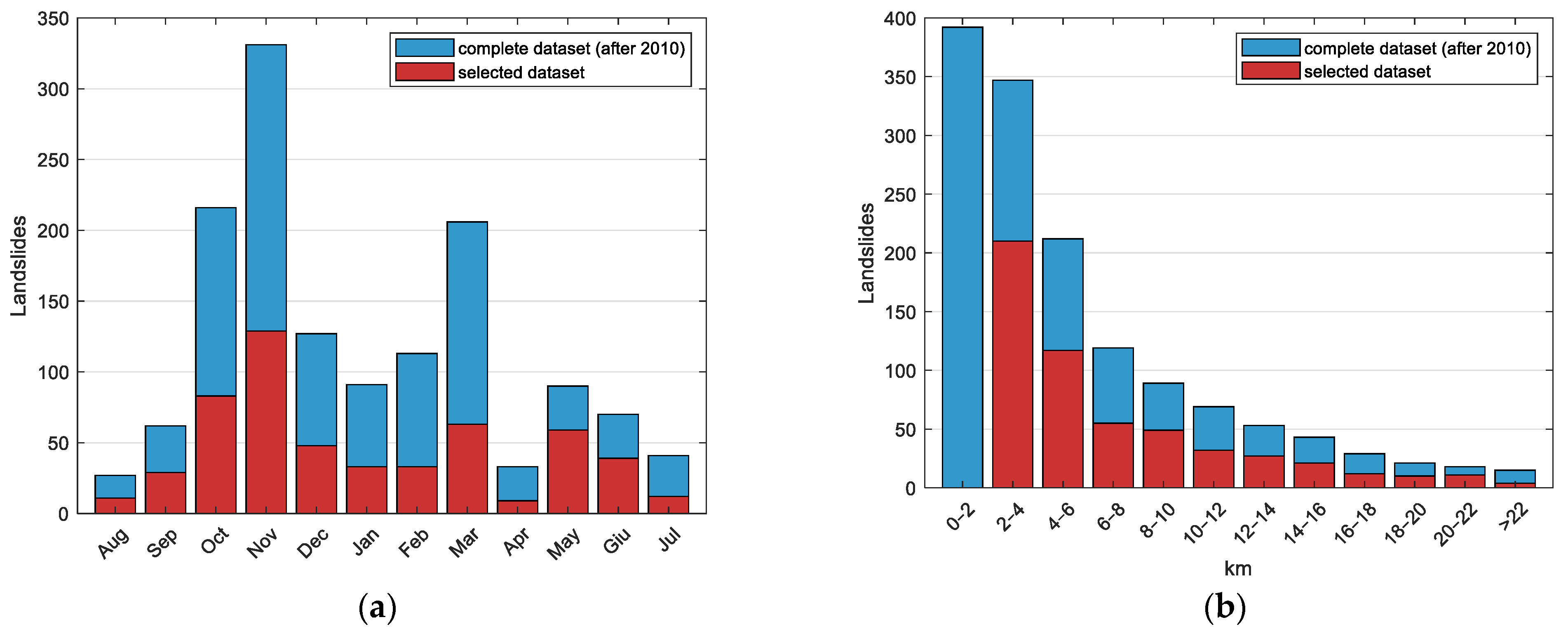
For this study, rainfall events associated with landslides were selected from the e-ITALICA v.4 catalog, based on the availability of radar data from 2010 onward. To reduce uncertainties and ensure high spatial and temporal accuracy, only landslides with high geographic and temporal precision were retained. This selection maximizes the reliability of landslide location and the estimation of the duration of the triggering rainfall event given the available data. Specifically, this included landslides with very high (P0) or high (P1, < 1 km²) spatial accuracy and precise knowledge of the event timing (hourly accuracy, T1). As a result of this filtering process, the dataset was reduced to 1550 landslides, of which 1407 have quantitative rainfall data available. These cases were then extracted from the e-ITALICA database for further analysis. Concerning the temporal distribution, more than 20% of rainfall-induced landslides occurred in November, followed by October and March.

To ensure the reliability of the analysis and the robustness of rainfall comparisons between the landslide site and the nearest rain gauge, a series of additional selection criteria were applied to the selected case studies. First, the distance between each landslide and its corresponding rain gauge, as indicated in the e-ITALICA database, was calculated using QGIS software. Only events with a minimum distance of 2 km were considered to ensure that the radar data, with a 1 km² spatial grid, could effectively differentiate rainfall between the two locations, avoiding spatial overlap and guaranteeing independent sampling. Cases between 1 and 2 km represent approximately 17% of the dataset, indicating that the applied threshold does not exclude a dominant portion of the observations. Next, to ensure that the radar-derived rainfall data provided a sufficiently complete representation of the triggering rainfall event, only cases where the hydrograph derived from the radar product covered at least 90% of the event’s duration were considered. This results in 771 events suitable for analysis. This requirement represents the main source of data reduction, as it ensures a robust estimation of rainfall accumulations.

In addition, a quality control step was implemented to assess the reliability of the radar estimates. The cumulative rainfall derived from the radar product within the grid cell containing the rain gauge was compared with the observed rainfall data recorded by the gauge itself, as reported in the e-ITALICA landslide database. Radar–gauge discrepancies arise from multiple sources, including measurement uncertainties, spatial rainfall variability, and the intrinsic mismatch between areal radar estimates and point rain gauge observations [47,48]. This last factor alone often explains a substantial fraction of the observed variability [47]. In the present study, a factor-of-10 threshold was adopted as a conservative and pragmatic criterion to identify discrepancies that are considered unlikely to represent typical radar–gauge differences and are more plausibly associated with artifacts such as beam blockage, calibration errors, or anomalous propagation. Although no universally accepted quantitative threshold exists in the literature, this choice is consistent with the general range of variability reported in radar–gauge intercomparison studies [47,48,49,50], and is intended to isolate extreme and physically implausible deviations while minimizing the exclusion of meaningful data. With this criterion, slightly less than 9% of the data were excluded, indicating that such cases are limited in frequency and represent a minor portion of the dataset.

Finally, a visual inspection of the spatial patterns in the radar-derived rainfall fields was performed for each landslide event. Radar rainfall accumulations in the area surrounding the landslide, including the grid cell containing the associated rain gauge, were checked to exclude events displaying artifacts, such as residual clutter or effects from the radar mosaicking process.

By applying these criteria, only radar data deemed sufficiently accurate were retained, ensuring that the subsequent analysis of rainfall discrepancies between the landslide site and the rain gauge location was based on reliable, artifact-free data. This process resulted in a final dataset of 548 rainfall events, which were used for further analysis.

Figure 1 shows the monthly distribution and distance classes of the 1407 landslides with high spatial and temporal accuracy available in the e-ITALICA database after 2010, together with the 548 events retained after the quality control procedure. The comparison indicates that, despite the reduction in sample size, the overall distribution shapes remain consistent, suggesting that the selection procedure does not introduce systematic biases in the temporal or spatial representativeness of the dataset.

3.2. Landslide–Rain Gauge Discrepancies Evaluation

For each considered landslide event, radar-derived rainfall accumulations were reconstructed from the SRI products, available at a temporal resolution Δt. Denoting by $SRI\left(t_k\right)$ the radar-estimated precipitation intensity at time $t_k$, the mean intensity between two consecutive time steps was calculated as:

$$\overline{SRI}(t_k)={\displaystyle \frac{SRI\left(t_k\right)+SRI\left(t_{k+1}\right)}{2}}, [\mathrm{mm}/\mathrm{h}]$$

(1)

and converted into partial accumulation E over the interval $∆t$:

$$E_{∆t}\left(t_k\right)=\overline{SRI}\left(t_k\right) ∆t, [\mathrm{mm}]$$

(2)

The total accumulation associated with the event was then obtained by summing all partial contributions:

$$E={\sum }_{k=1}^N{E}_{∆t}\left(t_k\right), [\mathrm{mm}]$$

(3)

where $N$ is the number of intervals $∆t$ required to adequately cover the total event duration $D$. To determine these intervals, all radar observations falling within the event window defined by the landslide occurrence time and the reported event duration were included. The accumulation starts from the first available record preceding the beginning of the event period and ending with the first record following the landslide occurrence. The main outputs of the procedure are the two radar-based accumulation estimates: $E_L$, corresponding to the grid cell containing the landslide, and $E_G$, corresponding to the grid cell containing the nearest available rain gauge to the landslide.

The comparison between the two radar-based accumulation estimates forms the core of the analysis. To minimize the influence of uncertainties in radar Quantitative Precipitation Estimation (QPE), the ratio

$$K={\displaystyle \frac{E_L}{E_G}},$$

(4)

was introduced, to quantify the relative discrepancy between the radar estimates in the two cells. This approach effectively allows to disregard potential multiplicative correction factors in the radar data: even if such factors vary spatially, assuming that these biases remain similar over the short distances involved (a few kilometers), their effect is reduced when computing the ratio. Furthermore, since the study focuses on rainfall events significant enough to trigger landslides, any radar additive biases are reasonably expected to be negligible compared to the radar signal. Thus, in this framework, the ratio (4) serves as a robust measure to characterize rainfall at the landslide site relative to the rain gauge site, allowing consistent analysis without the need for additional radar correction procedures. Values of (4) close to 1 indicate a strong agreement between the rainfall at the rain gauge and at the landslide site, while values significantly deviating from 1 represent either a positive or negative difference, depending on whether the rainfall at the landslide site is greater or smaller than at the gauge location. To treat relative increases and decreases symmetrically, the logarithm of the ratio (4) was considered. Since no systematic over- or underestimation is expected between the two cells, it is reasonable to assume that the sign of the discrepancy is random, reflecting the stochastic nature of the precipitation field. Thus, the absolute value of the logarithm of the ratio (4) was adopted as a proxy for the spatial variability of radar-estimated rainfall between the rain gauge location and the landslide site, and used for the analysis:

$$V=\left|{log}_{10}\left(K\right)\right|.$$

(5)

Higher values of $V$ indicate larger variation between the two radar estimates and therefore a higher degree of spatial variability of rainfall. This formulation expresses discrepancies in logarithmic space, i.e., in terms of orders of magnitude; consequently, values greater than 1 correspond to differences exceeding a factor of 10. Moreover, this formulation ensures equal weighting for discrepancies of the same magnitude, regardless of direction.

From a statistical perspective, it is reasonable to expect that $V$ increases, on average, with the distance $L$ between the landslide and the associated rain gauge. This relationship should not be interpreted in a deterministic or strictly monotonic sense: for individual events, $V$ may be small even at large distances, and vice versa. However, as $L$ increases, the probability of observing large discrepancies is expected to rise, due to the reduced spatial representativeness of more distant rain gauges with respect to the local rainfall at the landslide site.

To investigate this relationship, the data were grouped into distance classes, and for each class, the distribution of (5) was represented using boxplots. Differences among the distributions associated with the various classes were assessed using the non-parametric Kruskal–Wallis test [51], which evaluates the null hypothesis that samples originate from the same distribution without assuming normality, making it suitable for potentially skewed data with pronounced tails. When global significance was detected, a post hoc analysis was performed using Dunn’s test with Bonferroni correction to control the Type I error rate (i.e., false positives) in multiple comparisons [52]. This procedure enabled pairwise comparisons among distance classes, identifying which distributions differed significantly and highlighting possible trends with increasing distance.

To characterize the tails of the distribution of (5), the empirical Complementary Cumulative Distribution Function (CCDF) was estimated from the data. The CCDF is defined as the probability of observing values greater than a given threshold $x$:

$$CCDF\left(x\right)=P(V>x).$$

(6)

This approach allows for the characterization of the probability of large discrepancies, which represent the most relevant cases in assessing the representativeness of rain gauges with respect to local rainfall at landslide sites. The empirical CCDF, directly estimated from the data, also enables robust comparison of distribution tails across different distance classes, without assuming any predefined parametric form.

Finally, the potential influence of rainfall type on the distribution of $V$ was investigated. It is reasonable to expect that, at equal distance, convective events, which are characterized by greater spatial variability, may produce larger discrepancies compared to more spatially uniform stratiform precipitation. Since a direct classification of the rainfall events associated with the landslides was not available in the e-ITALICA database, a seasonal proxy was adopted. This choice is supported by the findings of [53,54], who showed that in the Mediterranean area convective precipitation in summer is substantially higher than stratiform precipitation. In addition, a study on precipitation in Sicily (southern Italy) [55] indicates that stratiform events occur more frequently than convective ones, particularly during winter and spring, whereas from summer to mid-autumn convective events contribute more to the total rainfall depth. Landslide events were divided into two subsets: May–September, corresponding to the period with a higher likelihood of convective activity, and October–April, predominantly associated with stratiform precipitation. For each subset, the distributions of $V$ across distance classes and the corresponding CCDFs were analyzed to assess whether systematic differences emerge between the two groups.

4. Results and Analysis

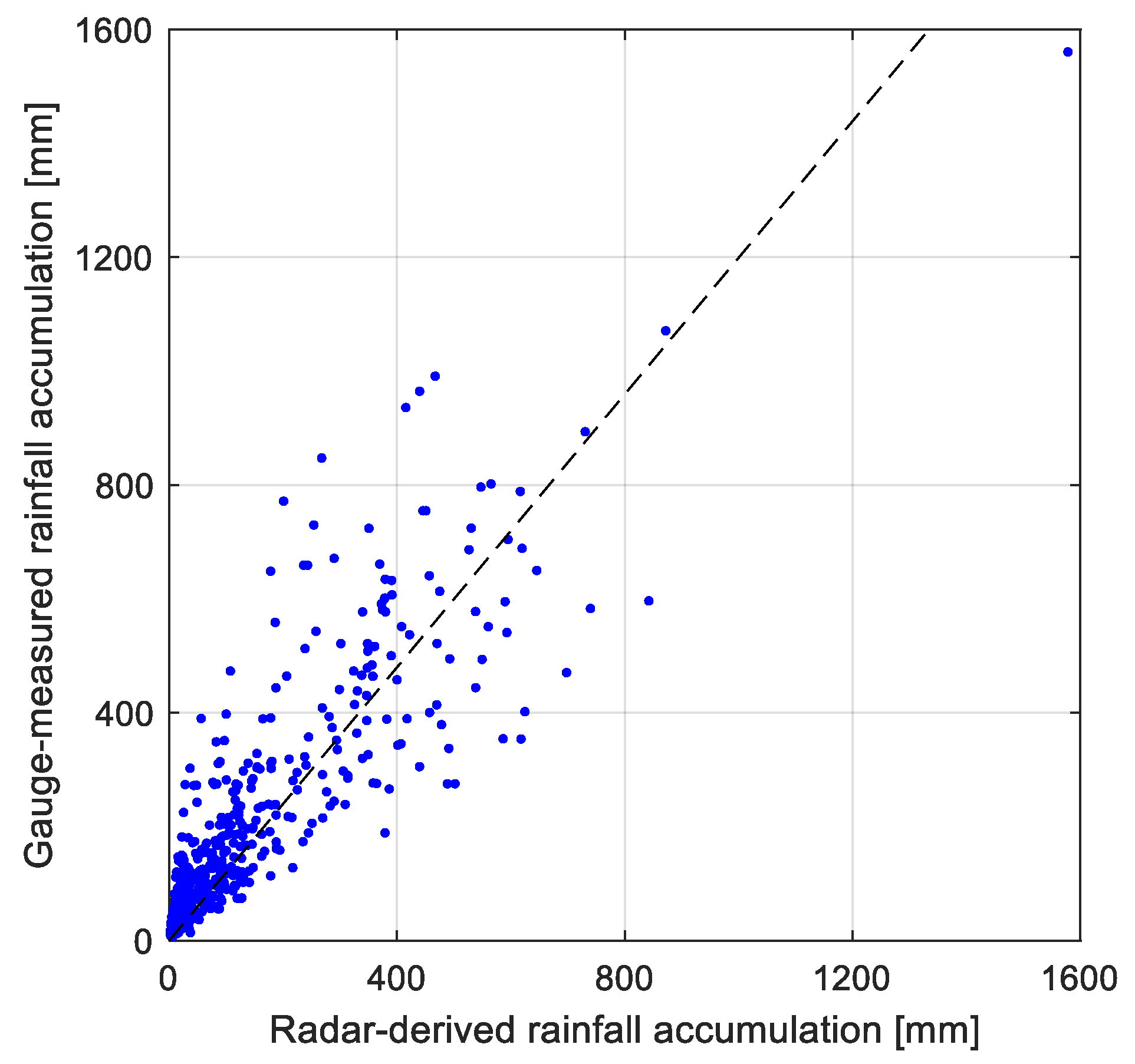
Based on the information available in the e-ITALICA database, an initial check on the reliability of the radar precipitation estimates was performed. For each record, the database provides the duration of the triggering rainfall event, the location of the nearest rain gauge, and the corresponding cumulative rainfall measured by the gauge. This enabled a comparison between radar-derived rainfall for the grid cell containing the rain gauge and the corresponding ground-based measurements.

The result of this comparison is shown in Figure 2 as a scatterplot, where each point represents a single event, with radar-estimated rainfall on the x-axis and the corresponding rainfall measured by the rain gauge on the y-axis. The graph also includes the best-fit line of the form Y = M X, obtained through least squares minimization. The scatterplot shows a good correlation between the two rainfall values at the national scale and for the events considered, with a slight average underestimation by the radar, as indicated by the slope of the best-fit line (M ≅ 1.2, coefficient of determination: $R^2\cong 0.7$). The Pearson correlation between radar-derived and rain gauge measurements is 0.86, which is consistent with values commonly reported in the literature for radar–rain gauge comparisons. Different studies show that discrepancies between radar estimates and rain gauge measurements include both systematic and random components, and may persist even after bias correction [48,49,50], and are also influenced by atmospheric conditions and precipitation processes [56,57]. The variability shown in Figure 2 therefore appears to be consistent with expectations and can be interpreted as confirming the overall reliability of radar estimates at the spatial and temporal scales considered.

This pattern suggests that a multiplicative correction factor could, on average, improve the radar estimate in the situations considered here. However, in the present study, the use of the ratio between two radar estimates allows such multiplicative effects to be largely mitigated. Therefore, the direct use of radar-derived rainfall to compute the ratio between the landslide location and the corresponding rain gauge location is justified and avoids the need for additional calibration.

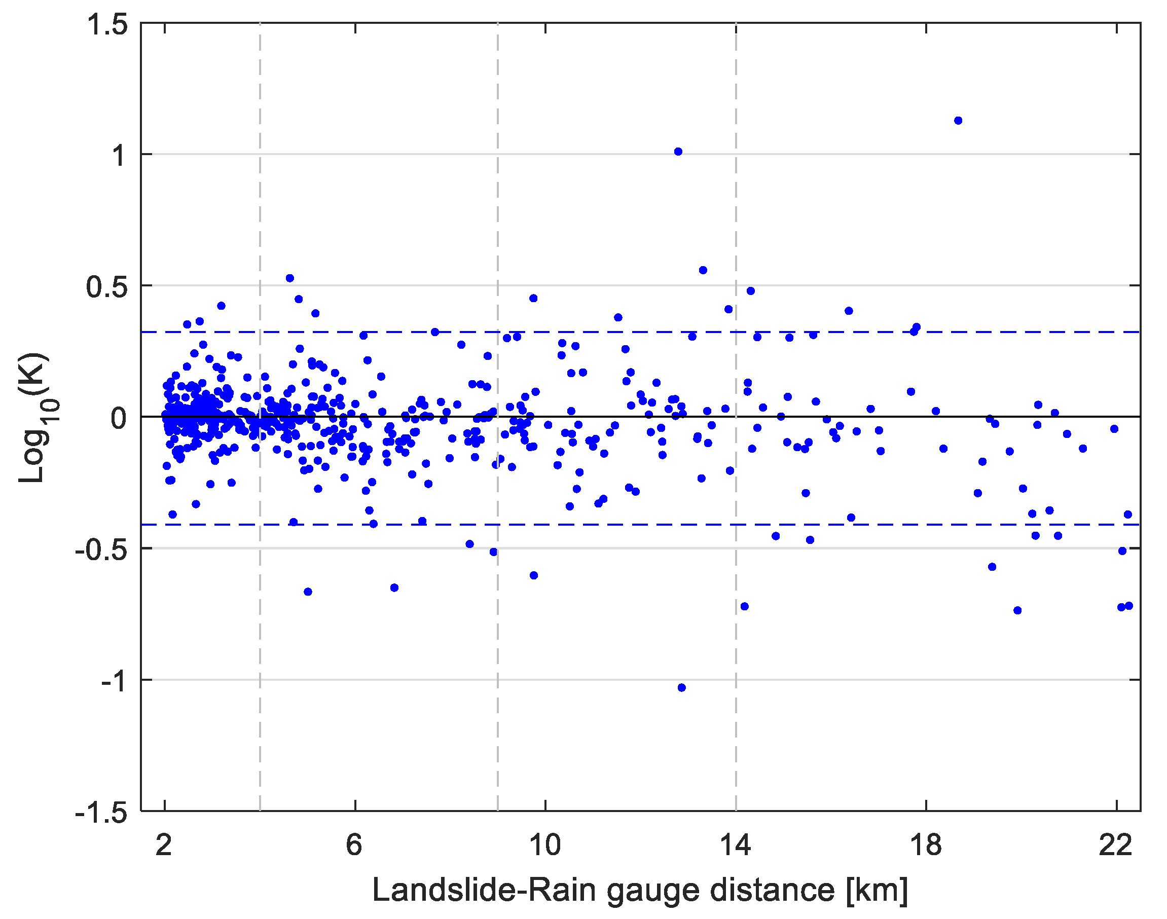
Figure 3 presents the scatterplot of the logarithm of the ratio (4) versus the landslide-to-gauge distance for the 548 landslide events analyzed. The logarithmic transformation allows a symmetrical representation of discrepancies, so that ratios above or below 1 are treated with equal magnitude but opposite signs, thus highlighting the magnitude of the discrepancy irrespective of its sign.

As expected, the points are distributed symmetrically around the x-axis (i.e., $K=1$), indicating the absence of a systematic over- or underestimation between the two locations being compared. This overall symmetry is confirmed by the summary statistics reported in

Table 1. Summary statistics of ${log}_{10}\left(K\right)$ considering all data.

Mean	Median	Standard Deviation	Skewness	Bowley
−0.0214	−0.0136	0.1833	−0.0643	−0.0948

, computed using all available ${log}_{10}\left(K\right)$ values irrespective of distance. In particular, the skewness (−0.06) and Bowley coefficient (−0.094), both very close to zero, indicate the nearly symmetrical nature of the overall distribution and suggest only a slight, negligible asymmetry that can reasonably be interpreted as a random fluctuation.

Consistently with the visual impression provided by Figure 3, the interquartile range shows that for 50% of the events the discrepancy between the two rainfall estimates remains within approximately 20%. However, the distribution also exhibits more extreme situations, as indicated by the 3rd and 97th percentiles, for which the discrepancy between the two estimates can be either less than half or more than double. These cases correspond to the points located far from the x-axis in Figure 3. These points occur at various values of distance. In fact, no deterministic or obvious monotonic trend with respect to distance emerges from Figure 3, in which values with greater discrepancies appear as possible outliers for each landslide-to-gauge distance.

To investigate potential systematic differences with distance, the data were grouped into classes. The definition of distance classes required particular attention due to the uneven data distribution, with a decreasing number of observations at larger distances. To ensure sufficient sample size in each class while preserving the ability to detect trends, four distance classes were defined, i.e., 2–4 km, 4–9 km, 9–14 km, and >14 km, containing 210, 198, 82, and 58 events, respectively. It is worth noting that the results presented in the following sections are robust with respect to the adopted classification. Alternative binning strategies were also tested, including equally spaced and equal-frequency (quantile-based) classes. While both approaches confirmed the overall behavior observed in the data, they present inherent limitations in this context: equally spaced classes lead to poorly populated bins at larger distances, reducing statistical reliability, whereas equal-frequency classes reduce spatial resolution by aggregating wide distance ranges at larger distances. The adopted classification was therefore selected as a compromise between statistical robustness and spatial resolution.

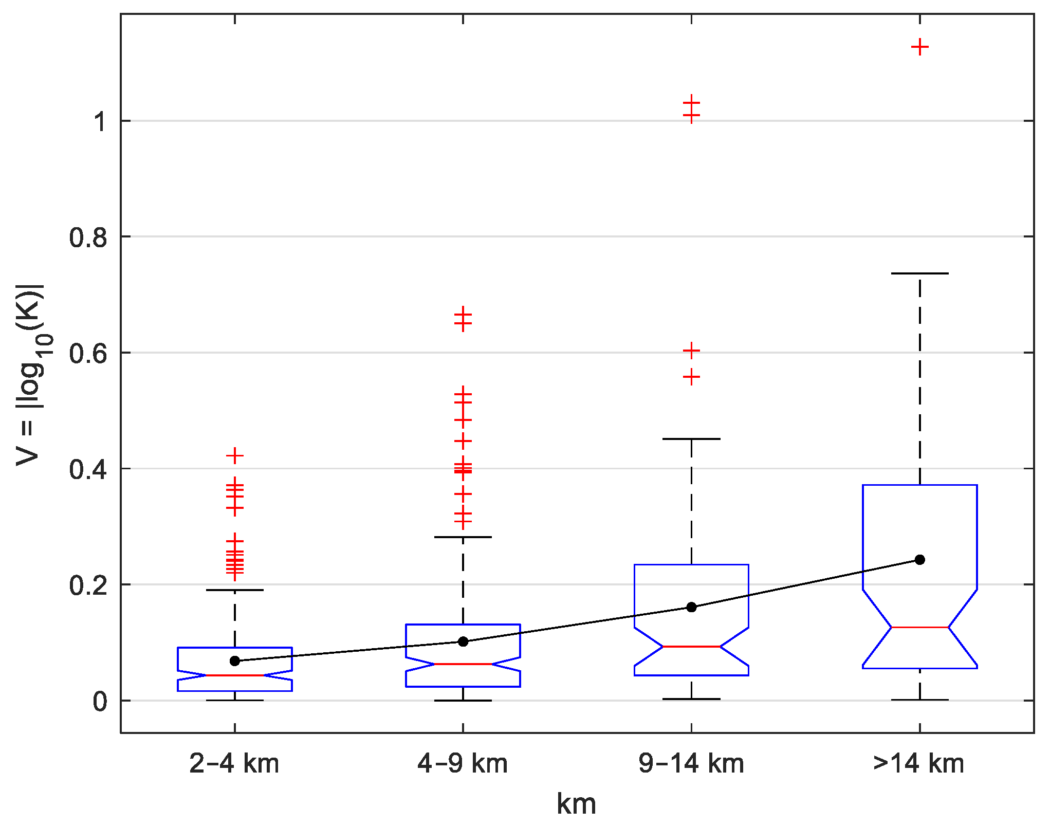
Figure 4 shows the boxplots of the distributions of the discrepancy metric (5) for the four chosen classes, while

Table 2. Summary statistics for the distributions of V, grouped into four distance classes, corresponding to the boxplots shown in Figure 4.

Distance Class	Sample Size	Mean	Median	Standard Deviation	Min	Max	Q1	Q3	97th
2–4 km	210	0.07	0.04	0.08	0.0001	0.42	0.02	0.09	0.26
4–9 km	198	0.10	0.06	0.12	0.0001	0.67	0.02	0.13	0.43
9–14 km	82	0.16	0.09	0.19	0.0028	1.03	0.04	0.23	0.62
>14 km	58	0.24	0.13	0.24	0.0012	1.13	0.06	0.37	0.73

summarizes their main statistical properties. The results indicate a progressive increase in dispersion with distance, reflected in the growth of the median, interquartile range, and upper percentiles. In particular, the right tail of the distribution becomes increasingly pronounced at larger distances, as highlighted by the increase in the third quartile and the 97th percentile. This behavior suggests that differences between rainfall estimates tend to become more significant as the distance increases.

To quantitatively assess the differences between the distributions of the four distance classes, a Kruskal–Wallis test [51] was performed, which returned a p-value significantly lower than 0.05, indicating that at least one of the distributions differs from the others. Subsequently, a post hoc test with Bonferroni correction for multiple comparisons [52] was conducted. The results show that the first three classes differ significantly from each other (1 vs. 2: p-value = 0.024; 1 vs. 3: p-value ~7.8·10⁻⁷; 2 vs. 3: p-value = 0.013), as do the more distant classes compared to the first ones (1 vs. 4: p-value ~8.8·10⁻¹⁰; 2 vs. 4: p-value ~4.9·10⁻⁵). In contrast, the difference between the third and fourth class is not significant (3 vs. 4: p-value = 0.748).

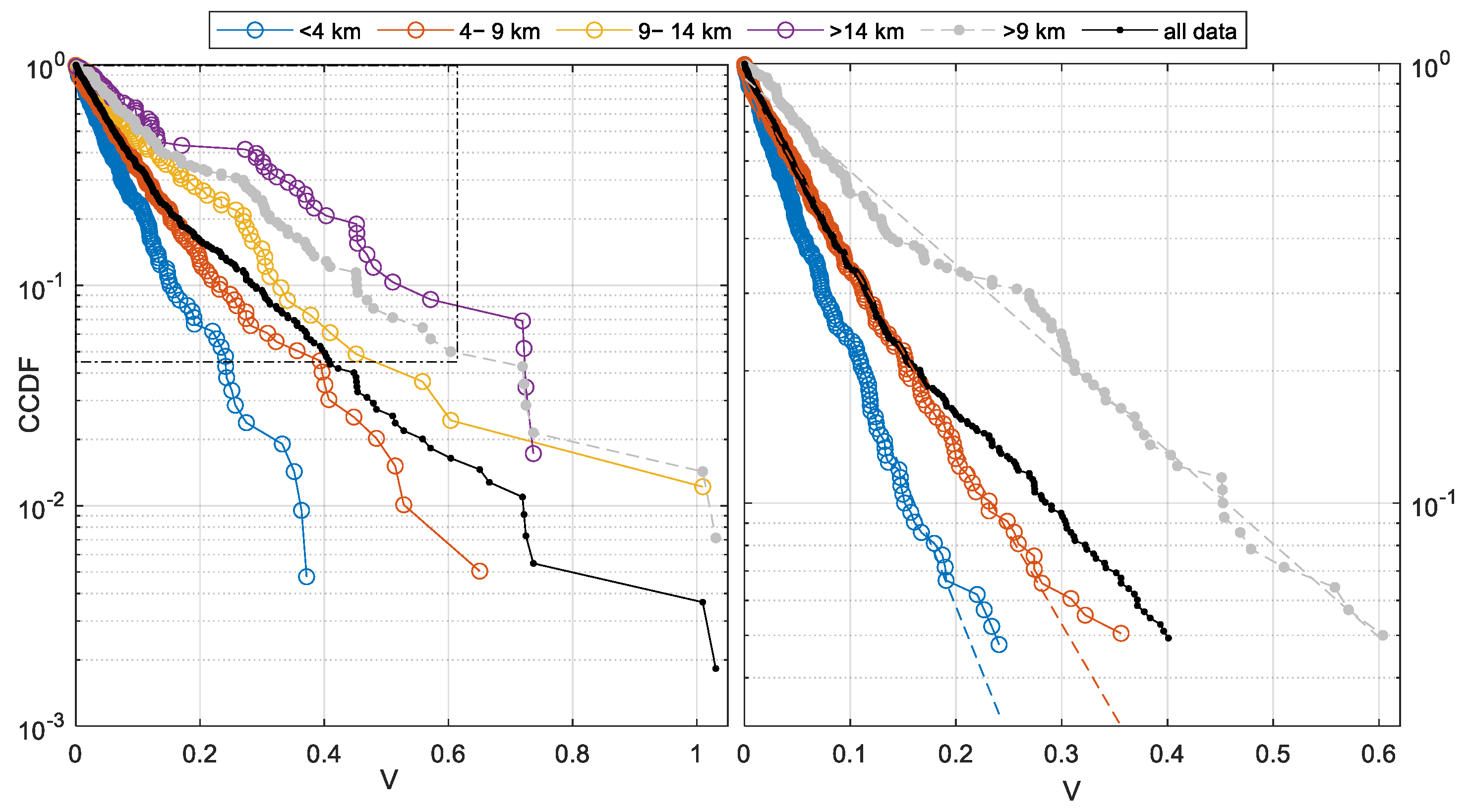
To further characterize the behavior of the distribution tails as a function of distance, the empirical complementary cumulative distribution functions (CCDFs) were calculated. These allow analysis of how the probability of exceeding a given threshold changes with distance. Figure 5 shows the overall CCDF (computed from the entire dataset) and the corresponding curves for the four distance classes, with the y-axis plotted on a logarithmic scale. The upper tail of an empirical CCDF is inevitably influenced by the limited sample size beyond a certain threshold. This effect is particularly evident for classes III (distances between 9 and 14 km) and IV (distances >14 km), which contain fewer events and therefore exhibit more pronounced fluctuations in the tails. To address this issue, Figure 5 also shows the CCDF obtained by aggregating data from these two classes, corresponding to events with a landslide–rain gauge distance greater than 9 km. In addition, the right panel presents a zoom where each curve is truncated at the 95th percentile, reducing fluctuations caused by limited sample size. This allows the main trends to be highlighted more clearly, minimizing noise-like fluctuations caused by the limited number of extreme points (for clarity, only the curve corresponding to the aggregation of classes III+ IV is shown).

Figure 5 indicates that all distance classes exhibit approximately linear trends on a semi-log scale, consistent with an exponential decay of the exceedance probability (6) of the form $~e^{-\lambda V}$. The $\lambda$ coefficients estimated from linear fits for the first two classes and the aggregated class are approximately 13.8, 9.5, and 4.9, with coefficients of determination of 0.990, 0.990, and 0.988, respectively.

This decay pattern is characteristic of a heavy-tailed distribution, which, as shown in Appendix A, can be associated with a Pareto distribution for the variable (4), with the shape parameter proportional to $\lambda$. The Pareto distribution [58] is known for its heavy tails, meaning that while extreme discrepancies between rainfall estimates at the two locations are rare, they are not negligible.

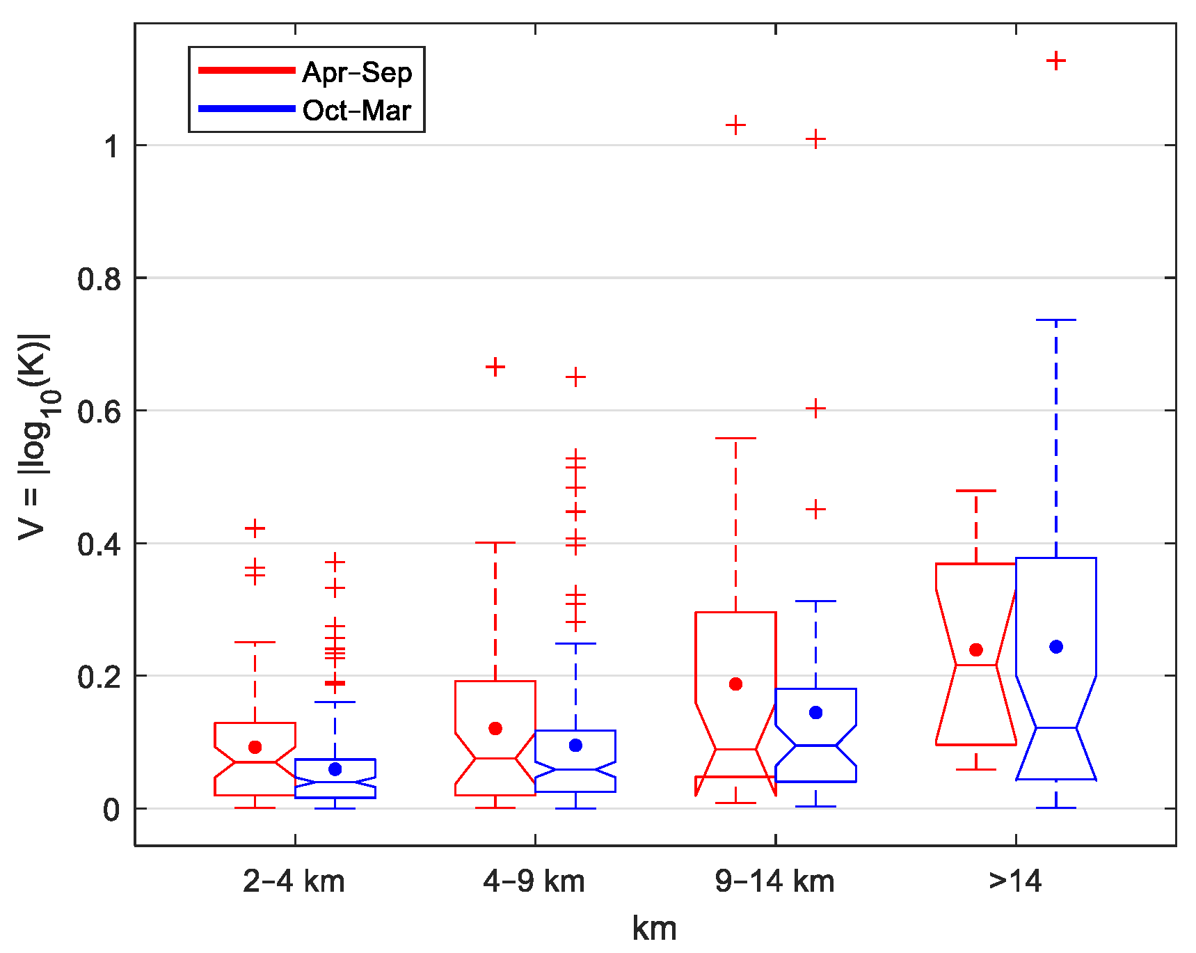
To investigate the effect of precipitation type (convective or stratiform) on the distribution of discrepancies, the dataset was divided into two seasonal periods: April–September (summer) and October–March (winter), chosen to ensure a sufficiently large number of events in both periods. This resulted in 150 events in the summer period and 398 in the winter period. Although this division does not guarantee a perfect separation between convective and stratiform events, it is reasonable to expect a predominance of convective events in summer and stratiform events in winter.

The data were then further divided into the same four distance classes that were previously used, resulting in 56, 49, 31, and 14 summer events, and 154, 149, 51, and 44 winter events for the respective classes. Histograms of the two V distributions were then calculated for each class. The results are shown in Figure 6, while a summary of the main statistical characteristics of the distributions is provided in

Table 3. Summary statistics for the distributions of V, grouped by season and distance classes, corresponding to the boxplots shown in Figure 6. For each distance class, the upper row corresponds to data for the Apr–Sep period, while the lower row corresponds to data for the Oct–Mar period.

Distance Class	Sample Size	Mean	Median	Standard Deviation	Min	Max	Q1	Q3	97th
2–4 km	56	0.09	0.07	0.10	0.00080	0.42	0.020	0.13	0.36
	154	0.06	0.04	0.07	0.00011	0.37	0.016	0.07	0.24
4–9 km	49	0.12	0.08	0.13	0.00054	0.67	0.020	0.19	0.41
	149	0.10	0.06	0.11	0.00009	0.65	0.025	0.12	0.45
9–14 km	31	0.19	0.09	0.21	0.0084	1.03	0.048	0.30	0.83
	51	0.14	0.09	0.17	0.0028	1.01	0.040	0.18	0.60
>14 km	14	0.24	0.22	0.16	0.0584	0.48	0.096	0.37	0.48
	44	0.24	0.12	0.26	0.0012	1.13	0.044	0.38	0.81

.

In the first distance class, the difference between the summer and winter distributions results statistically significant, with a p-value of 0.03 according to the Kruskal–Wallis test. In the subsequent classes, although no statistically significant differences were found, summer events consistently exhibit higher mean values and a longer right tail compared to winter events. Only in the last class (>14 km) the two distributions appear to largely overlap.

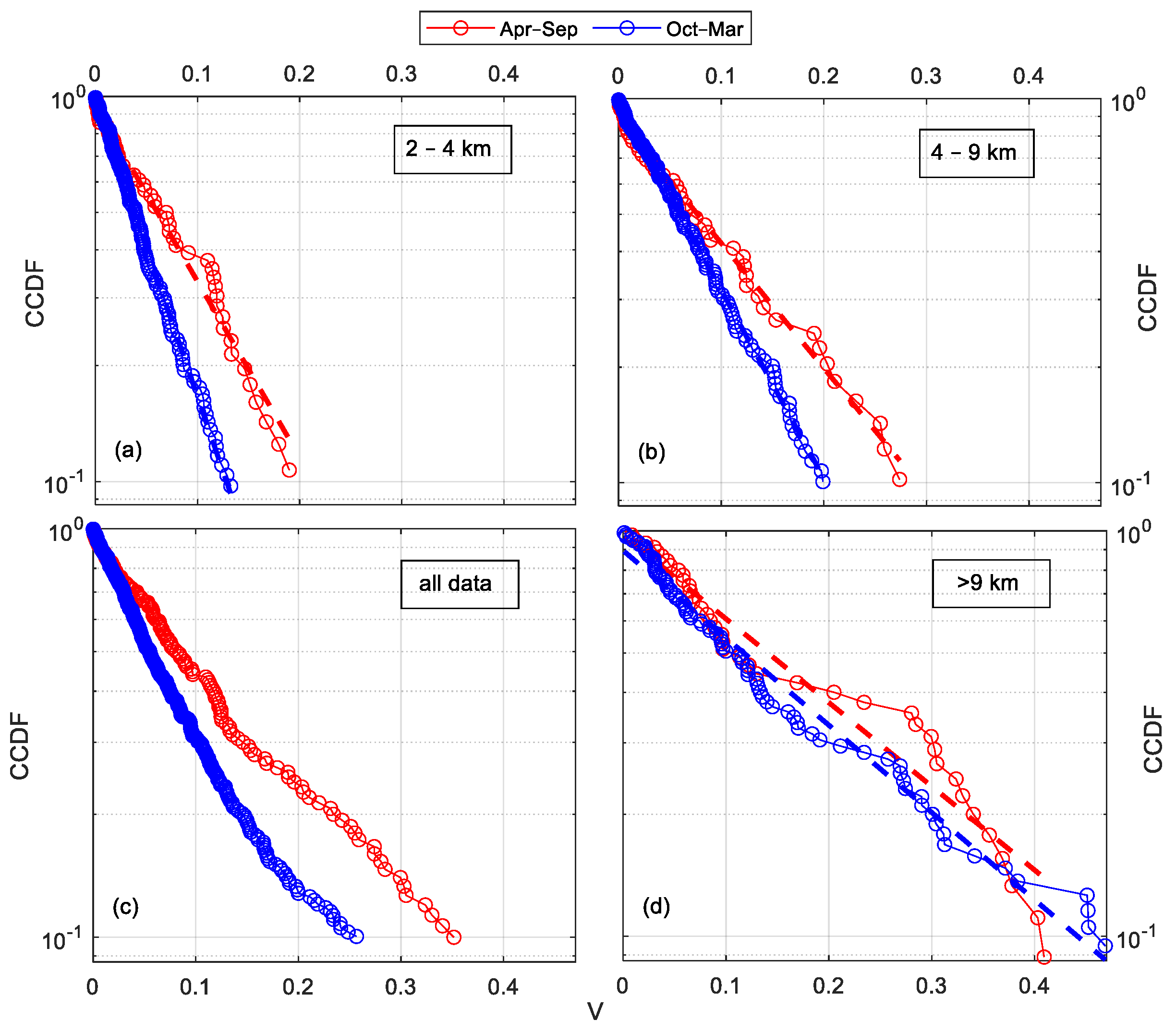
Finally, CCDFs were calculated for the two seasonal groups, both for the entire dataset and separately for the distance classes. In the latter case, the two largest distance classes were combined into a single class (>9 km) to increase the number of observations. The results are shown in Figure 7. Given the relatively small sample sizes, all curves were truncated at the 90th percentile to reduce statistically insignificant tail oscillations that could interfere with the visual interpretation of the trends.

Figure 7a,b,d show the CCDFs for the three distance classes considered (2–4 km, 4–9 km, >9 km, arranged clockwise from the top-left), while Figure 7c presents the CCDFs computed for all data. In all panels, blue curves correspond to winter events and red curves to summer events.

It can be seen that the curves are approximately linear, with slopes decreasing as the distance class increases. For the first two classes, the summer curves exhibit smaller slopes than the winter curves, indicating a slower decay of the probability of exceeding a given V value. In the largest distance class, the curves are more oscillatory due to the limited sample size, but essentially the same slope is observed. Specifically, denoting ${\lambda }_w$ and ${\lambda }_s$ as the slopes of the winter and summer curves, respectively, the following values are obtained: ${\lambda }_w=17.9$ and ${\lambda }_s=10.5$ for the class 2–4 km, ${\lambda }_w=11.3$ and ${\lambda }_s=7.5$ for the class 4–9 km, and ${\lambda }_w=5.0$ and ${\lambda }_s=4.8$ for the largest-distance class.

The CCDFs computed for the entire dataset summarize these results, confirming an approximately linear overall trend, with smaller slopes for summer events.

5. Discussion

The results indicate that distance influences rain gauge representativeness, but no monotonic or deterministic relationship emerges between distance and the magnitude of the discrepancy between the two rainfall estimates (Figure 3). At any distance, cases of close agreement between rainfall at the rain gauge and at the landslide location coexist with situations of substantial differences. Therefore, the effect of distance must be interpreted in probabilistic terms, by examining how the frequency and magnitude of discrepancies vary with distance through the statistical distribution of the observed values.

The analysis of the discrepancy distributions (Figure 5 and Figure 7) confirms that the tails of the distributions become progressively heavier as the distance class increases. As shown in Appendix A, the observed discrepancies are approximated by a Pareto distribution, which implies that, although events with large discrepancies are rare, they remain significant and have a non-negligible probability of occurring, especially as the distance between the landslide point and the rain gauge increases. In practical terms, this implies that rainfall estimates based on nearby gauges may occasionally deviate substantially from actual conditions at the landslide site, even at relatively short distances.

In fact, even at the shortest distance considered (2–4 km), notable differences can occur in some cases (Table 2). The median of index (5) corresponds to an error of about 4% between the two radar estimates considered, indicating close agreement for the most events. However, the third quartile already shows that this error rises to 23%, while the 97th percentile, which can be seen as a threshold for extreme cases, exceeds 80%. The situation worsens as distance increases. For half of the data, the median error rises to over 15%, 23%, and 35% across the successive distance classes. Moreover, for a quarter of the data from the second distance class onward, the error exceeds 35%. Extreme cases show errors exceeding 160% in the second class, reaching over 400% in the last class.

Importantly, this behavior is primarily driven by a limited number of extreme cases, which control the elongation of the right tail and increases both mean and median values, while most events show relatively similar rainfall estimates at the two locations. The observed increase in the median is statistically significant for the first three distance classes, as indicated by the notched boxplots, while differences between more distant classes become less pronounced. This may reflect either a saturation effect in spatial variability at larger distances or the reduced statistical power associated with smaller sample sizes.

The robustness of this behavior has been verified by testing alternative distance classifications, including different interval definitions and subdivisions into three and five classes. Across all configurations, the same general pattern emerges: distributions differ significantly at shorter distances, while differences become less distinct as distance increases. This consistency further supports the interpretation that the observed behavior is not an artifact of the chosen class definition, but rather reflects an intrinsic property of the data.

Further insight is provided by the analysis of the complementary cumulative distribution functions (CCDFs), which show that the probability of large discrepancies decays more slowly with increasing distance. The decrease in the parameter λ with distance indicates a slower decay in the probability of large discrepancies, i.e., more persistent tails in the V distribution. Some irregularities occur in the aggregated class, especially at high values. Nonetheless, the overall pattern is coherent and supports the interpretation of a systematic distance effect on extreme discrepancies.

Seasonal analysis highlights the effect of precipitation type (Table 3): summer precipitation, which is more likely to be convective, at the shortest distances actually show larger discrepancies than winter precipitation. The median discrepancy for summer events indicates an error of approximately 17%, compared to 10% for winter events, with the third quartile indicating that in a quarter of the cases, the error is already greater than 35% (compared to 17% for winter events). As the distance increases these differences progressively diminish.

These patterns highlight the role of precipitation type in controlling the spatial variability of rainfall. Convective events, which are more frequent in summer, indeed tend to produce higher discrepancies even at short distances, reflecting their inherently localized and spatially highly variable nature. Stratiform rainfall, on the other hand, generally produces more homogeneous rainfall fields, which typically require greater distances to give rise to situations with large discrepancies.

Therefore, the results emphasize that rain gauges, even when located relatively close to a landslide, may not always provide fully representative measurements. Although cases of large discrepancies are still rare, they are not negligible, and their frequency increases with distance, with convective rainfall amplifying these discrepancies even at short distances. Consequently, rainfall thresholds derived from rain gauges should take these findings into account to estimate potential errors in precipitation estimation, related to both the landslide–rain gauge distance and the type of rainfall event. In this sense, these findings highlight a limitation of purely gauge-based hydrological approaches, which may not fully capture the spatial variability of rainfall relevant for landslide triggering. At the same time, the statistical structure of the discrepancy distributions suggests that, while large deviations are not the dominant condition, their non-negligible probability makes them relevant for hazard assessment. The results therefore suggest that the use of distributed rainfall data, such as radar estimates, can substantially improve the characterization of triggering rainfall and reduce potential errors in landslide hazard assessment.

Despite the robustness of the proposed methodology and the consistency of the observed results, some limitations should be acknowledged to properly frame the scope of the study. The analysis is entirely based on radar-derived precipitation estimates, which are affected by multiple sources of uncertainty, including measurement errors, variability in reflectivity–rainfall relationships, beam blockage, and inconsistencies in radar mosaicking. In addition, intrinsic differences between areal radar observations and point rain gauge measurements inevitably introduce discrepancies. The ratio-based approach adopted here is specifically intended to reduce the impact of multiplicative biases, assuming that these are reasonably spatially coherent over short distances. If such uncertainties were the dominant source of the observed variability, a predominantly random pattern would be expected, with no systematic dependence on distance or consistent differences between rainfall regimes. In effect, known sources of radar bias are primarily related to radar-centric factors (e.g., range, beam geometry, and partial beam blockage), rather than to the distance between two arbitrary points on the ground, such as the landslide location and the nearest available rain gauge, making it physically implausible for such effects to generate the observed distance-dependent patterns. However, the results clearly depart from this expectation, revealing structured statistical patterns, including an increase in discrepancy with distance and distinct seasonal contrasts. These features are consistent with the well-established spatial organization of precipitation, characterized by a decay of correlation with distance [59] and fundamental differences between convective and stratiform precipitation systems [60], which exhibit markedly different spatial variability. Within this framework, the observed discrepancies are interpreted as primarily reflecting the intrinsic spatial variability of precipitation, while radar-related uncertainties are considered to play a secondary role. This interpretation is further supported by the theoretical analysis presented in Appendix B. Under general and physically plausible assumptions, residual bias variability can be modeled by treating the local gradient of the bias correction factor as a zero-mean random variable at the considered scales. This leads to a light-tailed perturbation, which cannot generate slowly decaying tails in the discrepancy distributions. Therefore, such uncertainties are expected to mainly contribute to increased noise in the discrepancy metrics, rather than to the emergence of the systematic structures observed in the results. At the same time, residual radar-related uncertainties cannot be completely excluded. Future developments could address this aspect by incorporating radar bias correction procedures based on rain gauge data or by adopting dedicated validation frameworks to quantify radar uncertainty across spatial scales.

Another limitation concerns the spatial resolution of the radar data (1 km²). Although this represents a significant improvement over point-based measurements, it may still be insufficient to fully capture sub-kilometer variability, particularly in the presence of convective cores. As a result, localized rainfall peaks may remain partially unresolved, potentially leading to an underestimation of rainfall variability at very short distances. Future studies could benefit from higher-resolution radar products or from the integration of complementary observations to better resolve fine-scale precipitation structures.

The definition of rainfall events is based on rain gauge data from the e-ITALICA database. While radar accumulations were reconstructed using time windows designed to fully encompass the reported events, minor inconsistencies in timing and structure between the two measurement systems may still occur. A possible improvement would be to define events directly from radar time series at landslide locations, allowing a more consistent comparison between radar- and gauge-based representations.

The interpretation of the results in terms of precipitation type relies on a seasonal classification used as a proxy for convective and stratiform regimes. Although this approach is supported by climatological evidence, it does not ensure a perfect separation between rainfall types, and some degree of misclassification is expected. Importantly, such uncertainty is likely to reduce the contrast between the two groups; therefore, the fact that statistically significant differences are observed despite this limitation suggests that the identified patterns are robust and may represent a conservative estimate of the actual differences. Future work could refine this aspect by adopting event-based classification methods based on radar signatures or atmospheric data.

Finally, the statistical analysis is influenced by the uneven distribution of sample sizes across distance classes, with fewer observations at larger distances. Although the robustness of the results has been verified through sensitivity analyses, conclusions, especially in distribution tails, should be interpreted cautiously for smaller subsets. This limitation could be mitigated in future studies by expanding the dataset.

The study also focuses exclusively on rainfall as a triggering factor, without explicitly accounting for antecedent conditions such as soil moisture or hydrological response. While this choice is consistent with the objective of assessing rainfall representativeness, it limits the direct applicability of the results to more complex landslide models. Future research could integrate additional hydrological variables to better capture the combined effects of rainfall and preconditioning factors on landslide initiation.

6. Conclusions

This study assessed the spatial representativeness of rain gauge measurements for rainfall-triggered landslides by comparing cumulative rainfall at landslide locations and at the nearest gauges, using radar-derived estimates at 1 km² resolution. The analysis, based on 548 events across Italy, quantifies how rainfall discrepancies vary with distance and precipitation type. Results show that distance influences rain gauge representativeness, but not deterministically. At all distances, close agreement and large discrepancies coexist, indicating that the effect of distance is inherently probabilistic. However, the likelihood and magnitude of large discrepancies increase with distance.

Discrepancy distributions exhibit progressively heavier tails with distance, consistent with Pareto-type behavior. This indicates that extreme discrepancies, although infrequent, are non-negligible and become increasingly relevant at larger distances. These extremes play a dominant role in shaping the distributions and summary statistics. Precipitation type further modulates these patterns. Convective events, more common in summer, generate larger discrepancies even at short distances, whereas stratiform precipitation, more frequent in winter, produces more homogeneous rainfall fields, with significant differences emerging mainly at larger distances.

Overall, rain gauges, even when located close to a landslide, may not always provide representative estimates of triggering rainfall. While large discrepancies are not the dominant condition, their non-negligible probability, especially under convective regimes, should be considered when deriving and applying rainfall thresholds. These findings support the use of spatially distributed rainfall products, such as radar estimates, to improve the characterization of triggering rainfall and reduce uncertainty in landslide hazard assessment. Future developments should focus on higher-resolution observations, radar–gauge integration, and improved discrimination between convective and stratiform precipitation.

Ultimately, this study highlights the need to move beyond point-based rainfall representations toward a more spatially explicit characterization of precipitation, to achieve more reliable and physically consistent landslide hazard assessments.