Satellite-Based Chlorophyll-a Prediction Reveals Salinity-Dominated Regime Shifts in the East China Sea: A 22-Year Multi-Sensor Analysis with Explainable AI

Highlights

What are the main findings?

• A geography-free XGBoost model achieves $R^2=0.802$ on 1.4 million satellite observations, and dual salinity thresholds (11.62 and 34.03 psu) mark ecological regime shifts missed by traditional physical definitions.
• The SSS Triple-Role Framework reveals that salinity serves as turbidity proxy, nutrient proxy, and dilution signal across the estuary-to-ocean gradient, resolving contradictory salinity effects.

What are the implications of the main finding?

• Non-additive SSS × SST coupling (61% modulation) demonstrates that climate warming effects on productivity depend on nutrient availability, requiring non-additive ecosystem models.
• Data-driven salinity thresholds extend the ecological Changjiang influence 20,000 ${\mathrm{km}}^2$ beyond physical definitions, providing operational benchmarks for satellite-based ecosystem monitoring.

Abstract

We developed an explainable machine learning framework combining 22 years (2003–2024) of multi-sensor satellite data (MODIS Aqua, CMEMS, C3S) with zone-specific SHAP attribution to quantify chlorophyll-a (Chl-a) mechanisms in the East China Sea. A geography-free XGBoost model achieved $R^2=0.802$ on 1.4 million pixel-month observations, and counterfactual experiments confirmed its superior environmental sensitivity over location-dependent models. Multi-strategy threshold detection identified two critical salinity boundaries—11.62 psu marking the turbidity-to-productivity transition (Cohen’s $d=-2.92$) and 34.03 psu at the Kuroshio Front ($d=-1.04$)—neither of which coincides with traditional physical definitions. Zone-specific SHAP analysis revealed that sea surface salinity (SSS) dominates Chl-a attribution across all zones but through fundamentally different mechanisms. We propose an “SSS Triple-Role Framework” in which salinity serves as turbidity proxy in estuarine waters, nutrient proxy in transitional waters, and dilution signal offshore, resolving the apparent contradiction of simultaneous positive and negative salinity effects. Non-additive interactions—including SSS × SST coupling (61% modulation) and SST × sea level amplification during Kuroshio intrusions—further demonstrate hierarchical controls missed by additive models. These findings provide quantitative benchmarks for ecosystem monitoring in river-dominated marginal seas.

1. Introduction

1.1. Background and Importance

Chlorophyll-a (Chl-a) concentration serves as a fundamental proxy for phytoplankton biomass and primary productivity in marine ecosystems, playing a critical role in biogeochemical cycling, fishery productivity, and ecosystem health assessment [1]. In coastal marginal seas, particularly those influenced by large river discharge, Chl-a dynamics exhibit pronounced spatial and temporal variability driven by complex interactions among physical, chemical, and biological processes [2,3]. The East China Sea (ECS), receiving massive freshwater and nutrient inputs from the Changjiang (Yangtze River)—the world’s third-largest river by discharge—represents an ideal natural laboratory for investigating how environmental gradients control phytoplankton productivity across river-dominated continental shelves [4,5,6]. The ECS circulation system, including the Changjiang Diluted Water, Taiwan Warm Current, and Kuroshio intrusion, creates a complex mosaic of nutrient supply and water mass mixing that modulates seasonal and interannual Chl-a variability [7,8]. Nutrient inputs from the Changjiang have been linked to recurrent phytoplankton blooms, hypoxia, and long-term eutrophication trends, underscoring the tight coupling between physical forcing and biological response in this system [9,10].

Satellite ocean color remote sensing has revolutionized our ability to monitor Chl-a dynamics at synoptic scales, with sensors such as MODIS Aqua providing continuous global coverage since 2002 [11]. However, translating satellite-derived Chl-a patterns into mechanistic understanding remains challenging, particularly in optically complex coastal waters where traditional bio-optical algorithms exhibit significant uncertainties [6]. The integration of multi-source satellite observations—encompassing ocean color, sea surface temperature (SST), sea surface salinity (SSS), sea level anomaly, and photosynthetically active radiation (PAR)—offers unprecedented opportunities to disentangle the environmental drivers of Chl-a variability across spatial gradients.

1.2. Challenges in Coastal Chl-a Prediction

Four fundamental challenges limit current understanding of ECS Chl-a dynamics. First, the transition from turbid estuarine to oligotrophic oceanic waters creates sharp environmental gradients where dominant drivers shift from sediment-modulated light availability to nutrient-limited productivity over distances of <100 km [12]. Traditional correlation-based analyses cannot capture these regime shifts because the same variable (e.g., salinity) may promote Chl-a in one region while suppressing it in another.

Second, environmental controls are fundamentally non-stationary across the estuary-to-ocean gradient: river discharge simultaneously affects turbidity, nutrient supply, stratification, and frontal dynamics, such that a single variable (e.g., SSS) can switch from promoting to suppressing Chl-a within a single study domain. The “nutrient-light paradox”—where nutrient-rich estuarine waters exhibit lower productivity than moderately diluted transitional waters—exemplifies how additive models fail in river-dominated systems [13].

Third, while machine learning models achieve high predictive accuracy for Chl-a [14,15], most operate as “black boxes” providing no mechanistic insight. Recent advances in explainable AI, particularly SHAP (SHapley Additive exPlanations) [16], offer a principled solution. SHAP is a game-theory-based attribution method that assigns each input variable a contribution score (Shapley value) for every individual prediction, thereby decomposing model outputs into additive feature effects and revealing which environmental drivers are responsible for predicted Chl-a variations at each pixel and time step. This approach has shown growing promise in environmental and oceanographic applications [17,18,19,20,21,22], enabling rigorous attribution of predictions to input features and bridging the gap between predictive power and ecological understanding.

Fourth, beyond identifying individual drivers, their pairwise non-additive interactions—such as how nutrient availability modulates temperature effects on phytoplankton growth, or how circulation regime alters the ecological meaning of warm water—remain poorly quantified in river-dominated systems, limiting our ability to predict ecosystem responses under compound environmental changes (e.g., concurrent warming and Kuroshio intensification).

1.3. Objectives

This study aims to understand the environmental mechanisms controlling chlorophyll-a variability across the East China Sea’s estuary-to-ocean gradient, with implications for ecosystem monitoring under climate change. Specifically, we address four objectives: (1) develop a geography-free machine learning model that learns transferable environment–Chl-a relationships rather than spatial memorization, enabling counterfactual reasoning about how environmental perturbations affect phytoplankton productivity; (2) quantify zone-specific driver hierarchies using SHAP attribution to reveal how the dominant controls on Chl-a shift from turbidity-mediated processes in estuarine waters to nutrient dilution in offshore waters; (3) identify and validate critical salinity thresholds marking ecological regime shifts in Chl-a dynamics; and (4) characterize multi-scale environmental interactions—such as nutrient-temperature coupling—that govern non-additive controls on phytoplankton productivity.

2. Materials and Methods

2.1. Study Area

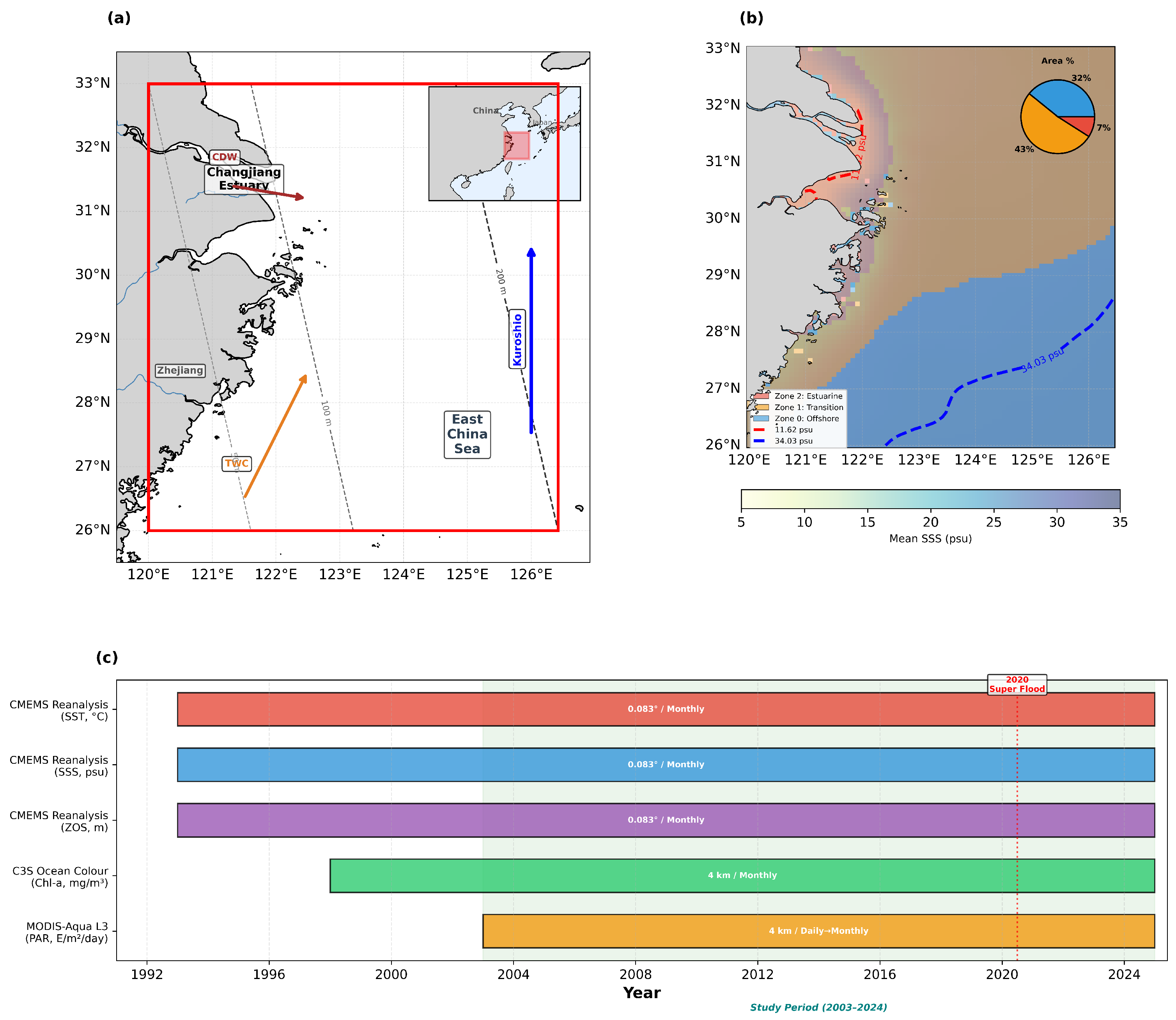
The East China Sea (120.00–126.42°E, 26.00–33.00°N) encompasses the Changjiang estuary, the broad continental shelf, and the Kuroshio Current influence zone (Figure 1). This region features dramatic environmental gradients: salinity ranges from <5 psu near the river mouth to >34 psu in Kuroshio-influenced waters, with corresponding transitions in turbidity, nutrient concentrations, and phytoplankton community structure. Three ecologically distinct zones were identified through K-means clustering of long-term mean salinity fields [23]: the estuarine zone (SSS range 5–28 psu, mean $17.73\pm 7.12$), the transition zone (28–32 psu, mean $31.63\pm 0.89$), and the offshore zone (>32 psu, mean $33.78\pm 0.45$) (The K-means algorithm assigned numeric labels (Zones 2, 1, and 0) based on cluster centroid ordering rather than geographic sequence; for clarity, we use descriptive names throughout and provide numeric equivalents where needed for cross-referencing with figures). Detailed zone characteristics are summarized in

Table 1. Ecological zone characteristics identified through K-means clustering of satellite environmental features in the East China Sea (2003–2024). SSS: sea surface salinity; SST: sea surface temperature.

Zone	Depth (m)	SSS Range (psu)	Mean SSS ± SD	Mean SST ± SD (°C)
Estuarine (Zone 2)	<50	5–28	17.73 ± 7.12	17.93 ± 4.82
Transition (Zone 1)	50–100	28–32	31.63 ± 0.89	19.87 ± 3.21
Offshore (Zone 0)	>100	>32	33.78 ± 0.45	24.03 ± 2.76

. Across the 22-year study period, the dataset contained 44,017 valid pixel-month observations in the estuarine zone (4.1% of total), 592,084 in the transition zone (55.2%), and 436,587 in the offshore zone (40.7%), totaling 1,072,688 Chl-a records (see Supplementary Table S1 for annual breakdown). The lower observation count in the Estuarine zone reflects both its smaller spatial extent and higher data loss due to cloud contamination and optical complexity in turbid nearshore waters.

2.2. Multi-Source Satellite Data

Six environmental features were derived from multi-source satellite and reanalysis products spanning 2003–2024 at monthly temporal resolution. All variables used in this study are monthly mean fields, which integrate the full diurnal cycle and sub-monthly variability:

Sea surface temperature (SST) was obtained from CMEMS Global Ocean Physics Reanalysis (GLORYS12V1, 0.083°), a gap-free product that assimilates in situ and satellite observations through data assimilation. Sea surface salinity (SSS) was sourced from the same CMEMS reanalysis product; SSS exhibits relatively low diurnal variability compared to SST and PAR, and monthly averaging further suppresses sub-monthly fluctuations. Sea level anomaly (ZOS) was derived from CMEMS GLORYS12V1 reanalysis, which assimilates satellite altimetry (e.g., Jason and Sentinel-3) and in situ measurements; the monthly mean product captures seasonal steric height variations, mesoscale circulation features including Kuroshio intrusion events (which typically persist for weeks to months), and geostrophic current anomalies but does not resolve tidal signals or storm surges, which are filtered during the reanalysis process. Photosynthetically active radiation (PAR) was obtained from MODIS-Aqua Level-3 monthly composites (9 km resolution), derived from daytime overpasses (∼1:30 PM local equatorial crossing time). Unlike the gap-free reanalysis products (SST, SSS, and ZOS), MODIS-Aqua PAR retains observational gaps due to cloud contamination—particularly severe during the ECS mei-yu season—that monthly compositing may not fully resolve. Furthermore, PAR represents surface (above-water) irradiance, not underwater light availability; in the turbid estuarine zone where euphotic depth can be <3 m, surface PAR is a poor proxy for the light actually available to phytoplankton. Seasonality was encoded as cyclical features using $sin(2\pi \times \mathrm{month}/12)$ and $cos(2\pi \times \mathrm{month}/12)$.

At the monthly temporal resolution employed here, the analysis can resolve seasonal cycles, interannual variability, monsoon-driven salinity changes, and Kuroshio intrusion events lasting weeks to months. However, sub-monthly bloom dynamics (which can peak and decay within 1–2 weeks), tidal-scale mixing events, diurnal PAR and SST cycles, and transient storm effects cannot be captured. The monthly resolution therefore acts as a low-pass filter that may dampen short-lived but ecologically significant events.

Chl-a concentration, the prediction target, was obtained from the C3S (Copernicus Climate Change Service) Ocean Colour merged satellite product at 9 km monthly resolution. Chl-a values were log-transformed using $\ln (1+\text{Chl-a})$ prior to all analyses to reduce right-skewness and stabilize variance, consistent with the log-normal distribution characteristic of coastal Chl-a. All datasets were regridded to a common 9 km grid using bilinear interpolation.

2.3. Geography-Free Feature Design

A critical innovation of this study is the exclusion of spatial coordinates (latitude and longitude) asmodel input features, forcing the algorithm to learn relationships between Chl-a and environmental conditions rather than geographic memorization. We term this design “geography-free” to describe the model architecture: the XGBoost model receives only environmental variables and has no access to spatial location during training or prediction. This design enables: (1) detection of transferable mechanisms operating across spatial gradients; (2) robustness during extreme events when spatial patterns shift; and (3) physically interpretable SHAP attributions reflecting environmental rather than positional effects. We note that the subsequent zone-specific SHAP interpretation (Section 2.5) deliberately reintroduces spatial context by stratifying results across ecologically defined zones. This stratification is an analytical choice for post hoc interpretation, not a model feature—the model itself remains geography-free throughout.

2.4. XGBoost Configuration and Training

XGBoost (eXtreme Gradient Boosting) [24] is an ensemble machine learning algorithm that builds a sequence of decision trees, where each successive tree corrects the residual errors of the preceding ones through gradient optimization. It was selected for its demonstrated effectiveness in environmental remote sensing applications [25] and its ability to capture nonlinear relationships, handle missing data, and provide built-in feature importance metrics. The model was implemented using the XGBoost Python library (v2.0.0) with hyperparameters optimized through Optuna Bayesian optimization with 5-fold cross-validation (mean CV $R^2=0.863$; see

Table 2. XGBoost hyperparameters used in the geography-free Chl-a prediction model, optimized through Optuna Bayesian optimization with 5-fold cross-validation (mean CV $R^2=0.863$).

Hyperparameter	Value	Description
n_estimators	3937	Final boosting rounds after early stopping
max_depth	5	Maximum tree depth
learning_rate	0.018	Learning rate ($\eta$)
subsample	0.697	Sample fraction per tree
colsample_bytree	0.843	Feature fraction per tree
min_child_weight	28	Minimum child weight
gamma	0.039	Minimum loss reduction
reg_alpha	0.052	L1 regularization
reg_lambda	0.287	L2 regularization
objective	reg:squarederror	Regression objective
random_state	42	Random seed

for details).

The total dataset comprised 1,423,366 valid pixel-month observations after removing land pixels and missing values from the original 1,437,744 entries. The dataset was split temporally: training on 2003–2019 ($n=\mathrm{1,099,621}$) and independent testing on 2020–2024 ($n=\mathrm{323,745}$), ensuring no temporal leakage. This split deliberately places the extreme 2020 Changjiang flood [26] in the test period to evaluate robustness under unprecedented conditions.

2.5. SHAP Attribution Framework

TreeSHAP [27] was applied to compute exact Shapley values for all predictions, enabling: (1) global feature importance ranking via mean $|{\varphi }_i|$; (2) zone-specific attribution through spatial aggregation; (3) dependence analysis revealing nonlinear feature–response relationships; and (4) interaction detection quantifying non-additive effects. TreeSHAP has $O\left(TL{D}^2\right)$ complexity per sample (where T is the number of trees, L the maximum leaves, and D the depth), making full-dataset computation on $n=\mathrm{1,423,366}$ observations with $T=3937$ trees prohibitively expensive. SHAP values were therefore computed on a stratified random subsample of 5000 observations, preserving the zone distribution of the full dataset. We verified subsample stability by computing SHAP values across five sample sizes (1000 to 20,000) with five independent random draws each. Global feature importance rankings were perfectly consistent across all 25 runs (SSS > ZOS > SST; Spearman $\rho =1.000$ between $n=5000$ and $n=\mathrm{20,000}$), with SSS normalized importance varying by <1% (range: 0.464–0.469). The coefficient of variation decreased from 1.2% at $n=1000$ to 0.2% at $n=\mathrm{20,000}$, confirming that the 5000-sample subset provides stable estimates for all reported attribution metrics. All SHAP-derived statistics reported hereafter (feature importance, dependence plots, interaction analyses) are based on this subsample unless otherwise noted.

To examine how the same environmental variable operates through different mechanisms across distinct ecological settings, SHAP analysis was conducted independently for each of the three K-means-defined zones (Section 2.1). This zone-stratified interpretation enables detection of mechanism transitions across the salinity gradient. We emphasize that this stratification is a post hoc analytical choice—the underlying XGBoost model remains geography-free throughout (Section 2.3), and the zone labels are used only to partition SHAP results for interpretation, not as model inputs.

2.6. Threshold Detection

Threshold detection was applied to sea surface salinity (SSS) as it was identified as the dominant driver of Chl-a attribution across all zones (Section 3.2). The ecological motivation is to identify critical salinity boundaries that mark regime shifts in phytoplankton productivity—specifically, the turbidity-to-productivity transition in the estuarine environment (where salt-induced flocculation releases phytoplankton from light limitation) and the Kuroshio front boundary (where oligotrophic oceanic water begins to suppress nutrient-driven productivity). A multi-strategy approach combined: (1) SHAP gradient analysis identifying inflection points in the SSS–SHAP response curve, which indicate salinity values where the ecological role of SSS changes abruptly; (2) Welch’s t-tests comparing SHAP distributions across candidate thresholds to assess whether the regime shift is statistically significant; (3) Cohen’s d effect sizes quantifying the ecological magnitude of regime shifts beyond mere statistical significance—a large $\left|d\right|$ indicates that the threshold separates fundamentally different Chl-a regimes, not just statistically distinguishable ones; and (4) non-parametric Mann–Whitney U tests providing robustness verification independent of distributional assumptions and sample size imbalance. Bootstrap resampling (1000 iterations) provided 95% confidence intervals for threshold location.

3. Results

3.1. Model Performance and Validation

The geography-free XGBoost model achieved strong predictive performance ($R^2=0.802$) despite excluding spatial coordinates—comparable to or exceeding recent Chl-a prediction studies in optically complex coastal waters that include geographic features [14,15]. Performance was consistent across zones, with $R^2$ ranging from 0.78 (offshore) to 0.83 (estuarine), demonstrating that environmental features alone can explain >80% of Chl-a variance without geographic information. Full training and testing metrics are presented in

Table 3. Model performance comparison between geography-free and +Location XGBoost models across training and testing conditions. RMSE and MAE are reported in original Chl-a space (${\mathrm{mg/m}}^3$) after back-transformation from $\ln (1+\text{Chl-a})$ predictions. $\Delta R^2$ represents change from training performance.

Model	Period	n	${\mathit{R}}^2$	RMSE (${\mathrm{mg/m}}^3$)	MAE (${\mathrm{mg/m}}^3$)	$\mathbf{\Delta }{\mathit{R}}^2$
Geo-Free	Train (2003–2019)	1,099,621	0.864	1.11	0.56	—
	Test (2020–2024)	323,745	0.802	1.32	0.68	−0.062
+Location	Train (2003–2019)	1,099,621	0.959	0.61	0.33	—
	Test (2020–2024)	323,745	0.954	0.64	0.36	−0.005

.

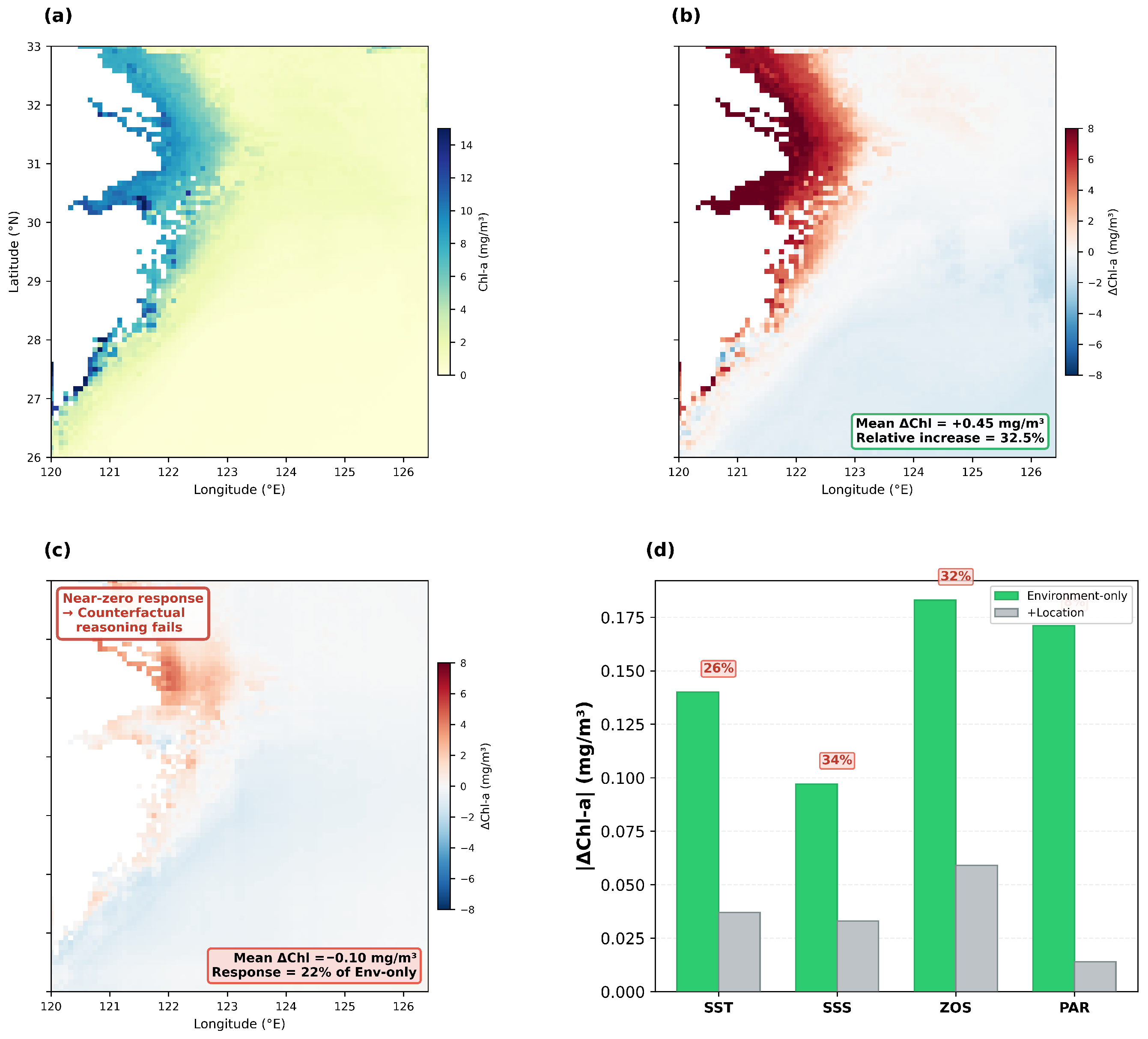
Critically, comparison with a location-dependent baseline model (with lat/lon features) revealed an instructive tradeoff between predictive accuracy and mechanistic interpretability (Table 3). The +Location model achieved higher overall test $R^2$ (0.954 versus 0.802), but counterfactual flood experiments (Figure 2) exposed its reliance on geographic memorization: when SSS was perturbed to 2020 flood conditions, the geography-free model responded with ecologically meaningful Chl-a increases in the estuarine zone, while the +Location model showed near-zero response—retaining only 4.6% of environmental sensitivity where it matters most. This demonstrates that high predictive $R^2$ can mask a fundamental failure of counterfactual reasoning: the +Location model learns “where” Chl-a is high by memorizing spatial patterns, not “why” it responds to environmental perturbations. Overall, the +Location model retained only 34.3% of the geography-free model’s counterfactual sensitivity in the 2020 flood scenario (

Table 4. Multi-scenario counterfactual experiments comparing geography-free and +Location model sensitivity. $\Delta$Chl values are reported in ln$(1+\text{Chl-a})$ space (the model’s native prediction space); percentage changes are computed accordingly. Sensitivity ratio indicates the fraction of geography-free response retained by the +Location model. All scenarios use paired t-tests at the pixel level.

Scenario	Perturbation	$\mathbf{\Delta }$${\mathrm{Chl}}_{\mathbf{GF}}$	% Change	ΔChl+Loc	Ratio	p-Value
2020 Extreme Flood	$\Delta$SSS → hist. mean	$+0.088$	$+5.2\%$	$+0.030$	34.3%	<0.001
Moderate Flood	$\Delta$SSS $=-5$ psu (estuarine)	$-0.036$	$-2.4\%$	$-0.011$	31.7%	<0.001
El Niño Warming	$\Delta$SST $=+{1.5 }^{\circ }$C (domain)	$+0.222$	$+10.6\%$	$+0.060$	27.1%	<0.001
Winter Storm	$\Delta$ZOS $=+0.15$ m (domain)	$-0.289$	$-11.1\%$	$-0.069$	24.0%	<0.001
Mean					29.3%

; note that Figure 2 reports $\Delta$Chl-a in original ${\mathrm{mg/m}}^3$ space while Table 4 reports values in the model’s native ln$(1+\text{Chl-a})$ space, accounting for numerical differences between the two). The feature-level sensitivity comparison (Figure 2d) reveals that this suppression varies by feature: PAR sensitivity is most severely compromised (8% retention), while SSS and ZOS retain approximately one-third of the geography-free response, indicating that geographic memorization disproportionately absorbs light-related variability.

To further validate the geography-free model’s environmental sensitivity beyond the 2020 extreme flood, we conducted multi-scenario counterfactual experiments spanning distinct perturbation types (Table 4). Perturbation magnitudes were chosen to reflect physically realistic anomalies: the moderate flood scenario ($\Delta$SSS $=-5$ psu in estuarine waters) corresponds to ∼1 SD of interannual SSS variability in Zone 2; El Niño-like warming ($\Delta$SST $=+{1.5 }^{\circ }$C domain-wide) approximates the ECS SST anomaly observed during strong El Niño events (e.g., 2015–2016) and aligns with near-term climate projections [28], and winter storm conditions ($\Delta$ZOS $=+0.15$ m) represent a typical Kuroshio intrusion-associated sea level perturbation in the ECS [29]. A synthetic moderate flood produced a 2.4% Chl-a response (paired $t=-12.8$, $p<0.001$), demonstrating sensitivity to sub-extreme freshwater events. El Niño-like warming yielded a $+10.6\%$ change ($p<0.001$), consistent with the SSS × SST hierarchical control identified in Section 3.6. Winter storm conditions produced a $-11.1\%$ response ($p<0.001$), confirming the model captures sea level-mediated Kuroshio effects. Across all four scenarios, the +Location model retained only 29% of the geography-free model’s counterfactual sensitivity on average (ranging from 24% for ZOS perturbations to 34% for SSS perturbations), reinforcing that spatial memorization suppresses counterfactual environmental reasoning regardless of perturbation type.

3.2. Global Feature Importance from Satellite Observations

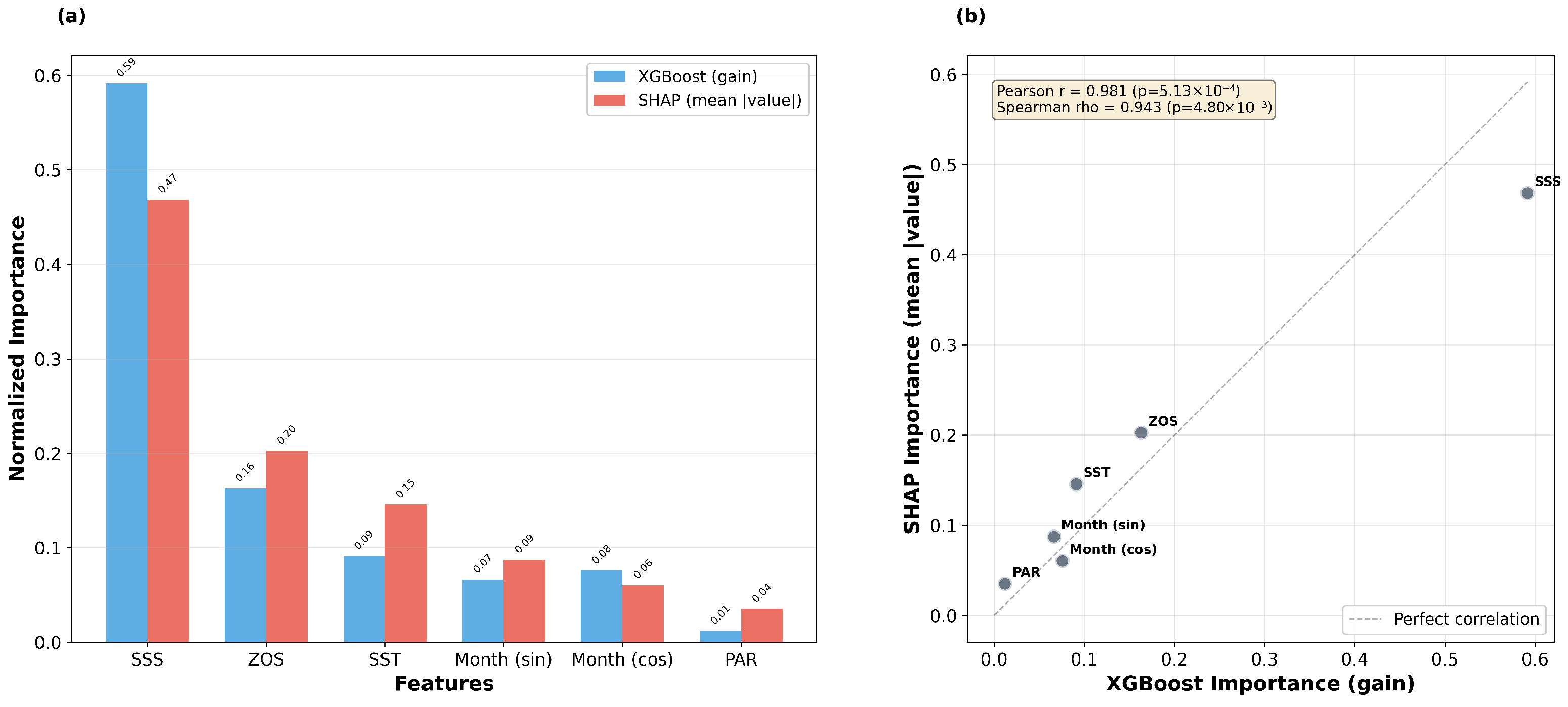
Global SHAP analysis across a stratified random subsample of 5000 pixel-month observations (from 1,423,366 total; see Section 2.5) revealed sea surface salinity as the overwhelmingly dominant driver of Chl-a variance, accounting for nearly half of total attribution (Figure 3a). This dominance was confirmed by strong agreement between SHAP-based and XGBoost gain-based importance rankings (Figure 3b), validating SHAP as a reliable attribution method for satellite-derived environmental drivers.

Secondary drivers followed a clear hierarchy: ZOS > SST > seasonal indicators > PAR. The unexpectedly low importance of PAR contradicts traditional light-limitation paradigms for estuarine systems. Rather than direct light availability controlling Chl-a variance, SSS appears to act as a “master proxy” encoding multiple co-varying processes—turbidity, nutrients, and stratification—that collectively govern the underwater light and nutrient environment more effectively than surface PAR alone. This “master proxy” role of SSS is further explored in the zone-specific analysis below and discussed in Section 4.4.

3.3. Zone-Specific SHAP Attribution

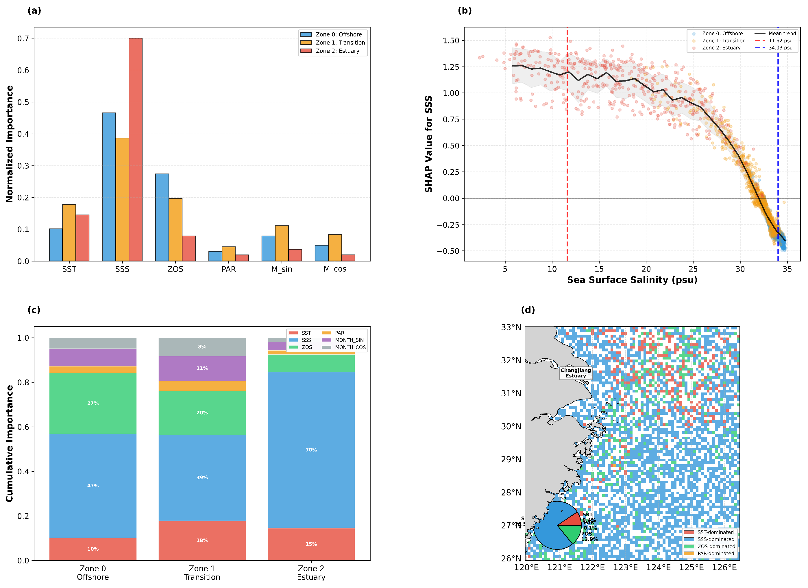
K-means clustering identified three ecologically distinct zones with markedly different driver hierarchies (Figure 4a,c;

Table 5. Zone-specific SHAP attribution analysis revealing spatial heterogeneity in environmental driver importance. Mean $\left|\mathrm{SHAP}\right|$ represents the average absolute SHAP value; contribution percentages sum to 100% within each zone.

	Zone 2 (Estuarine)		Zone 1 (Transition)		Zone 0 (Offshore)
Feature	$\left|\mathbf{SHAP}\right|$	Contrib.	$\left|\mathbf{SHAP}\right|$	Contrib.	$\left|\mathbf{SHAP}\right|$	Contrib.
SSS	1.026	70.0%	0.271	38.7%	0.315	46.7%
SST	0.213	14.6%	0.125	17.8%	0.067	10.0%
ZOS	0.116	7.9%	0.138	19.6%	0.185	27.5%
PAR	0.028	1.9%	0.031	4.4%	0.020	2.9%
Seasonality	0.083	5.7%	0.137	19.5%	0.087	12.9%

):

Zone 2 (Estuarine Core): SSS overwhelmingly dominated attribution, reflecting salinity’s role as a turbidity proxy in this highly turbid environment (suspended sediment > 500 mg/L). In these waters, Chl-a variability is governed primarily by when flocculation and sediment settling create windows of light availability for phytoplankton, rather than by direct light (PAR) or temperature fluctuations.

Zone 1 (Transition): A more balanced multi-driver structure emerged, with SSS, ZOS, SST, and seasonal indicators all contributing substantially (Table 5). This balanced attribution reflects the ecological character of the transition zone: light limitation has eased as turbidity declines seaward, but nutrients from the Changjiang remain available, creating conditions where multiple environmental factors jointly regulate Chl-a.

Zone 0 (Offshore): SSS remained the most important driver but with negative SHAP values, indicating that increasing salinity (Kuroshio intrusion) suppresses Chl-a through nutrient dilution. ZOS emerged as a strong secondary driver, consistent with the role of sea level anomalies in tracking Kuroshio intrusion events that bring warm, oligotrophic water onto the shelf.

The SSS SHAP dependence plot (Figure 4b) revealed a monotonically decreasing relationship across the full salinity gradient, with distinct zone separation—visually demonstrating the mechanism transition from SSS promoting Chl-a in estuarine waters (positive SHAP) to suppressing it offshore (negative SHAP). The pixel-level spatial dominant driver map (Figure 4d) confirmed SSS dominance across the majority of the study domain, with SST- and ZOS-dominated pixels concentrated near the Kuroshio boundary where oceanic circulation processes become the primary control on Chl-a.

3.4. Environmental Limitation Regimes

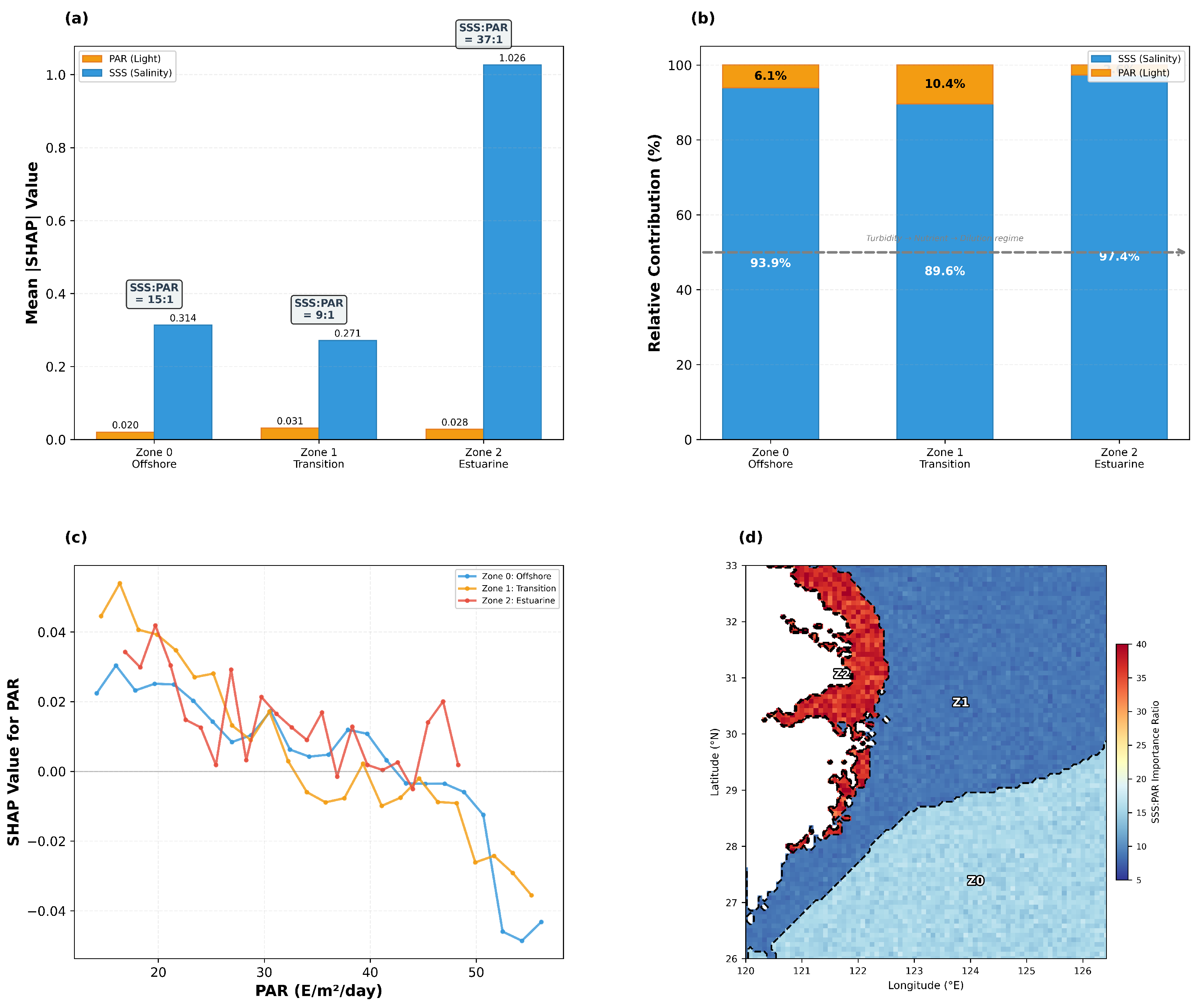
Quantitative limitation regime analysis compared PAR versus SSS importance to diagnose whether estuarine systems are light-limited or nutrient/turbidity-controlled (Figure 5a,b). To isolate the light-versus-salinity competition, SSS and PAR attributions were renormalized to sum to 100% (i.e., considering only the SSS–PAR pair). This pairwise comparison does not account for potential light information encoded in other features (e.g., seasonal indicators partially reflecting photoperiod); however, it provides a direct and interpretable contrast between the two most relevant proxies. The results decisively reject the light-limitation hypothesis across all three zones:

In the estuarine zone (Zone 2), SSS-mediated processes explain ∼37 times more Chl-a variance than direct light availability (Figure 5a). This aligns with physical oceanography: suspended sediment concentrations > 500 mg/L restrict euphotic depth to <3 m near the estuary [30,31], but Chl-a variability is governed by when flocculation releases phytoplankton from aggregates (salinity > 10 psu), not by PAR fluctuations. In the transition zone (Zone 1), the SSS:PAR ratio decreases as light limitation begins to ease seaward, but nutrient-mediated processes still dominate the Chl-a variance. In the offshore zone (Zone 0), SSS importance reflects Kuroshio nutrient dilution (negative effect) rather than turbidity, and light is rarely limiting despite deeper euphotic depths (Figure 5b).

The PAR SHAP dependence analysis (Figure 5c) revealed that all zones show a transition from positive SHAP values at low PAR to negative values at high PAR, consistent with photoinhibition at extreme irradiance. However, the magnitude was uniformly small compared to SSS effects, confirming that direct light availability plays a secondary role to salinity-mediated processes across the entire domain. We note that a data quality asymmetry may partially contribute to the low PAR attribution: unlike the gap-free reanalysis-based SST, SSS, and ZOS fields, MODIS-Aqua PAR is subject to cloud contamination—particularly severe during the ECS mei-yu season—that monthly compositing may not fully resolve. Additionally, because different levels of PAR can have different ecological effects depending on season (e.g., a given PAR level may be sufficient for growth in winter but not in spring), the monthly-averaged surface PAR used here cannot capture such context-dependent effects. Nevertheless, the physical argument that SSS proxies the underwater light field more effectively than surface PAR in turbid waters (where euphotic depth < 3 m) remains the primary explanation (see Section 4.4 for further discussion).

The spatial SSS:PAR importance ratio map (Figure 5d) visualizes the gradient from extreme SSS dominance near the coast to moderate dominance offshore, with zone boundaries clearly delineated by ratio transitions.

3.5. Salinity Threshold Detection and Validation

Multi-strategy threshold analysis identified two ecologically critical salinity boundaries with robust statistical support (Figure 6;

Table 6. Statistical validation of data-driven salinity thresholds identified through SHAP gradient analysis. Effect sizes quantified using Cohen’s d; significance assessed via Welch’s t-test.

Threshold	Detection Method	95% CI	Cohen’s d	p-Value	n (Below/Above)
11.62 psu	SHAP gradient peak	10.0–14.0	$-2.92$	<0.001 ***	95/4905
∼34 psu	SHAP local minimum	33.0–34.6	$-1.04$	<0.001 ***	4178/822
31 psu a	Physical definition	—	$-0.14$	$0.14$	1102/3898

^a Traditional 31 psu boundary; no detectable ecological signal. *** $p<0.001$. Sample sizes refer to the SHAP random subsample ($n=5000$); see Section 2.5. Non-parametric Mann–Whitney U tests confirmed both thresholds ($U=\mathrm{456,441}$ for 11.62 psu; $U=\mathrm{3,314,094}$ for ∼34 psu; both $p<0.001$), providing validation robust to sample size asymmetry.

):

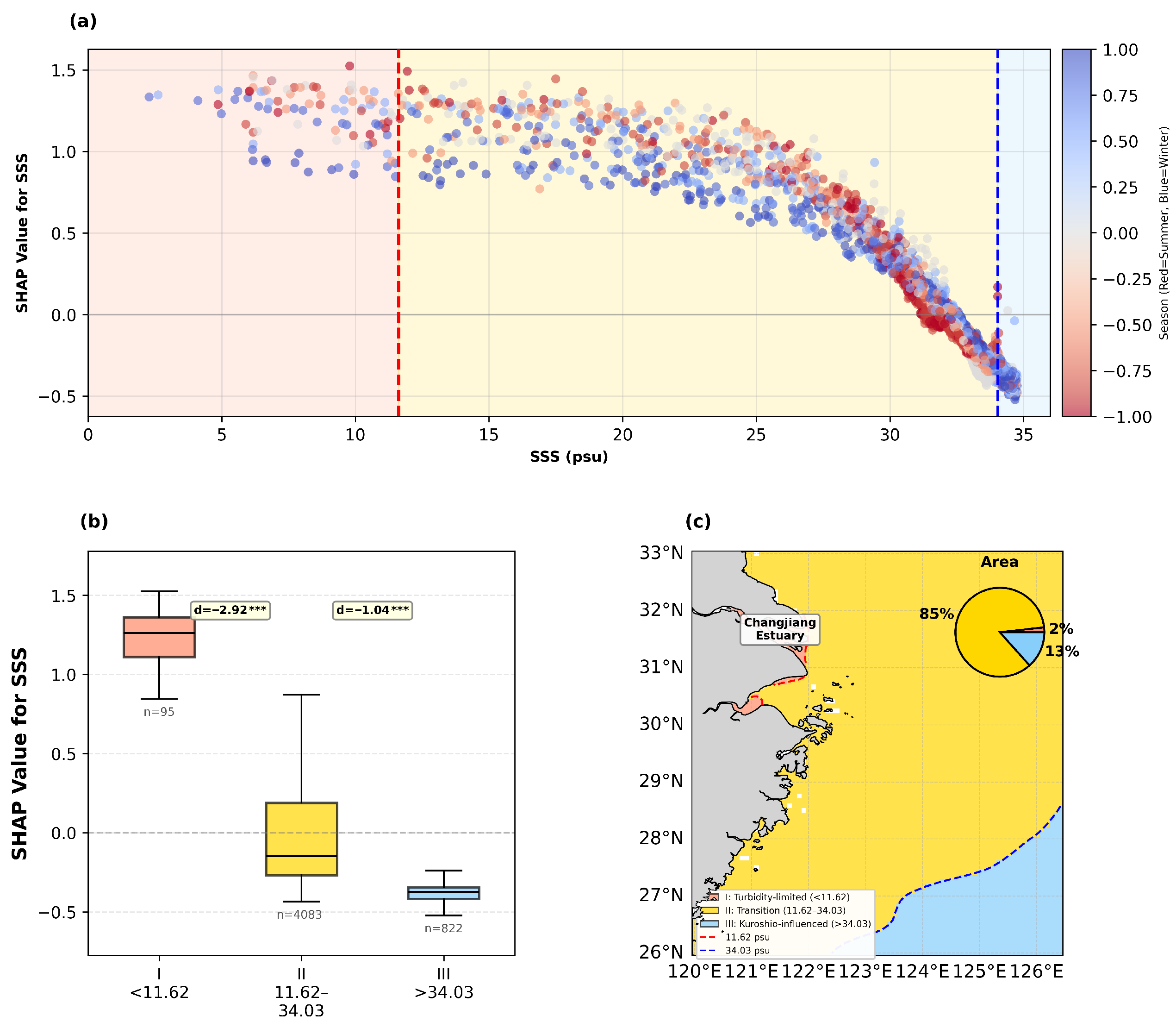
Low-salinity threshold (11.62 psu): SHAP gradient analysis revealed a prominent inflection in the SSS–Chl-a relationship at 11.62 psu, marking the turbidity-to-productivity transition. Below this threshold, high turbidity from riverine sediment suppresses phytoplankton productivity despite abundant nutrients; above it, salt-induced flocculation settles suspended particles and releases phytoplankton from light limitation, producing a 93% increase in mean Chl-a concentration. This ecological regime shift was confirmed by an extreme effect size (Cohen’s $d=-2.92$; Table 6), and the finding is consistent with recent observations of a salinity inflection near 10 psu at the estuarine turbidity maximum. The below-threshold group ($n=95$) is small, reflecting the genuine rarity of very low salinity observations in the 9 km gridded dataset (∼1.9% of the domain); robustness was verified using both non-parametric Mann–Whitney U tests and oversampling experiments (see Table 6 footnote for details).

High-salinity threshold (34.03 psu): A secondary inflection at the Kuroshio Front boundary ($d=-1.04$; Table 6) marks the transition from nutrient-supported to oligotrophic conditions. This threshold extends the ecological footprint of Changjiang influence ∼3 psu beyond the traditional 31 psu CDW physical boundary, encompassing approximately 20,000 ${\mathrm{km}}^2$ of additional ecologically productive area. Notably, the traditional 31 psu boundary showed no detectable ecological signal ($p=0.14$, $d=-0.14$; Table 6), underscoring the value of data-driven threshold detection.

The scatter plot with regime backgrounds (Figure 6a) demonstrated clear seasonal patterns: summer points (red) cluster in the low-salinity/high-SHAP region (CDW expansion), while winter points (blue) occupy the high-salinity/low-SHAP region. The spatial regime classification (Figure 6c) mapped three regimes based on mean SSS: Regime I (turbidity-limited, <11.62 psu, 2% area), Regime II (transition, 11.62–34.03 psu, 13% area), and Regime III (Kuroshio-influenced, >34.03 psu, 85% area).

3.6. Multi-Scale Environmental Interactions

SHAP interaction analysis revealed significant non-additive environmental couplings that traditional additive models cannot capture (Figure 7;

Table 7. Quantification of multi-scale environmental interactions detected through SHAP interaction analysis. Modulation percentage indicates relative effect size change between conditional states.

Interaction	Zone	Conditional State	Mean SHAP ± SD	Modulation
SSS × SST	Zone 1	Nutrient-rich (SSS < 32.6 psu)	0.313 ± 0.83	—
		Nutrient-depleted (SSS ≥ 32.6 psu)	0.123 ± 0.50	$-60.8\%$ ***
SST × ZOS	Zone 0	Low sea level (ZOS < 0.49 m)	−0.032 ± 0.05	—
		High sea level (ZOS ≥ 0.49 m)	−0.084 ± 0.06	×2.6 ***

*** $p<0.001$.

):

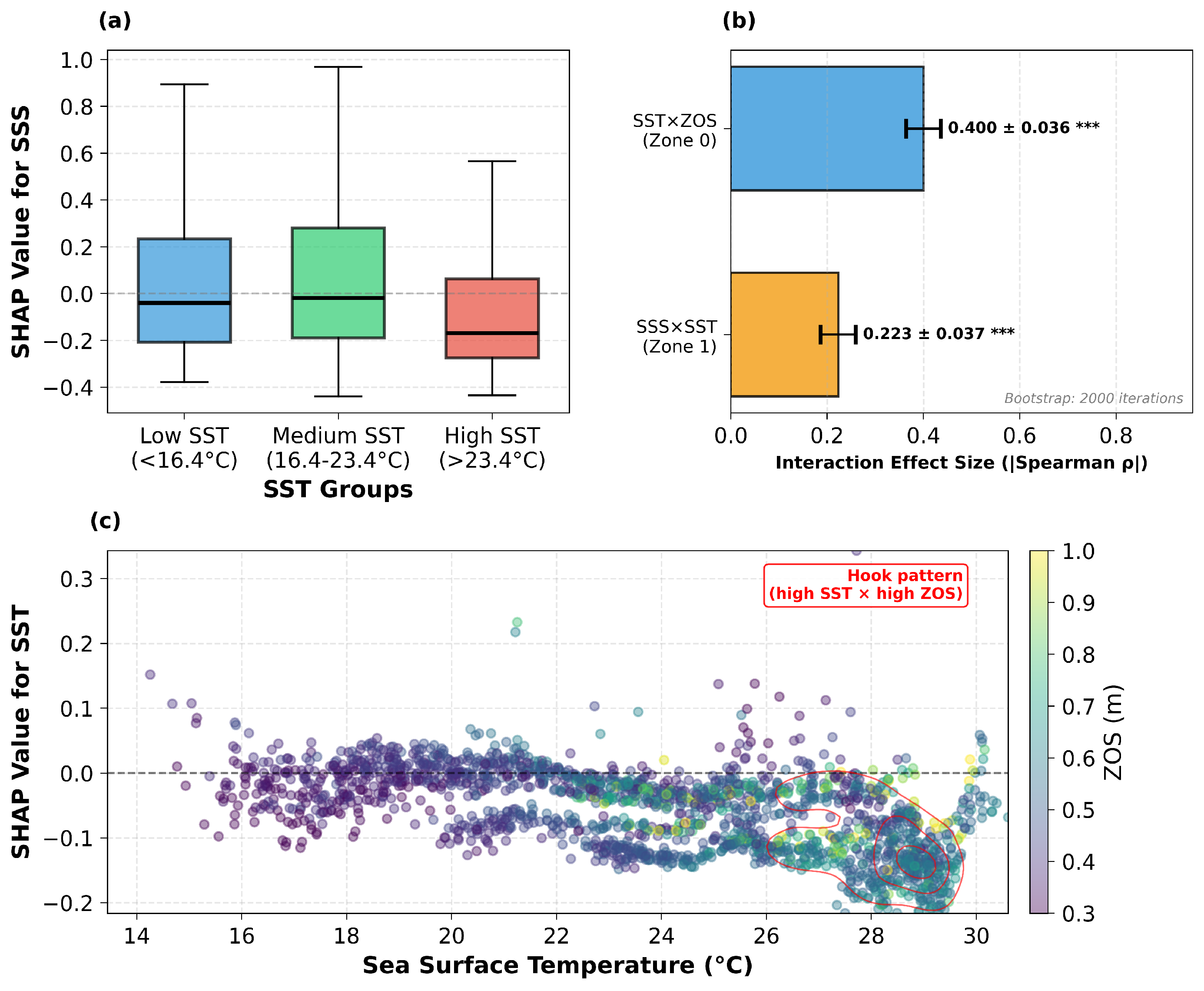
SSS × SST Interaction (Zone 1, Transition): Temperature effects on Chl-a are hierarchically controlled by nutrient availability. In the transition zone, warming accelerates phytoplankton growth rates and Chl-a accumulation—but only when nutrients are available to support increased metabolism. Under nutrient-rich conditions (lower SSS), the positive SST effect on Chl-a was ∼2.5 times stronger than under nutrient-depleted conditions, representing a 61% reduction in temperature importance when nutrients become limiting (Table 7). This hierarchical limitation was independently confirmed by SST-grouped analysis (Figure 7a), which showed significant differences in SSS SHAP values across temperature categories (Kruskal–Wallis $p<{10}^{-27}$). This finding has direct implications for climate projections: traditional additive models that assume uniform warming effects across nutrient gradients will systematically overestimate productivity gains in nutrient-poor waters.

SST×ZOS Interaction (Zone 0, Offshore): Warm water produces fundamentally different ecological outcomes depending on circulation context. Kuroshio-transported warm water (indicated by elevated ZOS) is oligotrophic, strongly suppressing Chl-a, while coastally retained warm water preserves terrestrial nutrients and has near-neutral Chl-a effects. The Kuroshio amplification of negative SST effects is quantified in Table 7, and a distinctive “hook pattern” in the SST–SHAP relationship (Figure 7c) reveals this mechanism visually: at equivalent high temperatures (>${27 }^{\circ }$C), SST SHAP values diverge sharply between high-ZOS (Kuroshio) and low-ZOS (coastal) conditions. This provides a satellite-detectable signature for identifying when Kuroshio intrusion events are suppressing shelf productivity.

4. Discussion

4.1. Methodological Advances in Satellite–AI Integration

This study demonstrates three methodological advances for coastal ecosystem analysis. First, the geography-free XGBoost framework learned transferable environmental relationships rather than geographic memorization, as validated by counterfactual experiments (Figure 2; Table 4). Although the +Location model achieved higher overall accuracy, it showed dramatically reduced sensitivity to environmental perturbations—demonstrating that high predictive $R^2$ can mask a fundamental failure of counterfactual reasoning. The +Location model predicts “where” Chl-a is high by memorizing spatial patterns, not “why” it responds to environmental perturbations. We note that these counterfactual perturbations test model-learned associations rather than true causal interventions; nevertheless, the geography-free model’s ability to respond appropriately to physically plausible environmental changes supports its utility for mechanistic attribution.

Second, SHAP attribution provided rigorous quantification of driver importance with zone-specific and interaction detection capabilities that correlation analysis cannot achieve. Third, multi-strategy threshold detection combining SHAP gradients, Welch’s t-tests, and Cohen’s d effect sizes ensured ecological boundaries are statistically robust rather than artifacts.

4.2. Ecological Significance of Dual Salinity Thresholds

The 11.62 psu threshold marks the turbidity-to-productivity transition where salt-induced flocculation releases phytoplankton from light limitation [32]. This mechanism, previously conceptual [33], is now quantified with extreme effect size ($d=-2.92$; Table 6). The threshold operates consistently over 22 years, confirming flocculation as an interannual-scale control. Critically, SSS proxies the underwater light environment better than satellite-derived PAR, explaining why direct light observations showed weak importance (1.9–4.4% of total attribution) across all zones.

The 34.03 psu threshold (bootstrap 95% CI: 33.0–34.6 psu) extends the ecological footprint of Changjiang influence ∼3 psu beyond the traditional 31 psu CDW physical boundary [23], encompassing 20,000 ${\mathrm{km}}^2$ additional area. We note that the relatively wide confidence interval reflects the gradual nature of the Kuroshio front transition; the precise threshold value should be interpreted as ∼34 psu rather than implying sub-psu precision. This discrepancy arises because nutrients persist beyond the physical front [34,35]; dissolved inorganic nitrogen and phosphate supplied by the Changjiang remain bioavailable well into the shelf region where physical salinity signatures have already been diluted [12,36,37]. The Kuroshio intrusion further modulates this extended boundary by supplying warm, oligotrophic water that sharpens the ecological gradient [29]. Notably, the traditional 31 psu threshold showed no ecological signal ($p=0.14$, $d=-0.14$), underscoring the value of data-driven over inherited definitions.

4.3. SSS Triple-Role Framework

While the multi-faceted role of salinity in river-influenced coastal systems has been qualitatively recognized—including its associations with turbidity [32], nutrient supply [34], and water mass mixing [23]—no prior study has quantitatively partitioned these roles using pixel-level attribution across a continuous salinity gradient. The most significant contribution of this study is the SHAP-based quantification showing that SSS plays three mechanistically distinct roles with sharply delineated transitions (Figure 8), forming a unified “SSS Triple-Role Framework”:

Role 1: Turbidity Proxy (Zone 2, SSS < 11.62 psu). In the estuarine core, low SSS indicates high freshwater input carrying massive sediment loads. SSS SHAP values are strongly positive (mean $=+1.026$), meaning that when salinity decreases (more river water), the model predicts higher Chl-a because flocculation-mediated light release dominates. Here, 100% of SHAP values are positive, and SSS acts as a proxy for the turbidity–light regime [38].

Role 2: Nutrient Proxy (Zone 1, 11.62–34.03 psu). In transitional waters, SSS reflects the balance between nutrient-rich river water and nutrient-poor oceanic water. SSS SHAP values are weakly positive (mean $=+0.040$), with only 40% of individual pixel-month SHAP values being positive (versus 100% in Zone 2), indicating that the SSS–Chl-a relationship is highly context-dependent in this zone. SSS here integrates nutrient supply and dilution signals, modulated by SST (61% interaction effect).

Role 3: Dilution Signal (Zone 0, SSS > 34.03 psu). In offshore waters, high SSS signals Kuroshio intrusion carrying warm, oligotrophic water. SSS SHAP values are negative (mean $=-0.310$), with only 2% positive, meaning that increasing salinity suppresses Chl-a through nutrient dilution. This “dilution paradox”—where more oceanic water reduces productivity—is consistently captured by the model.

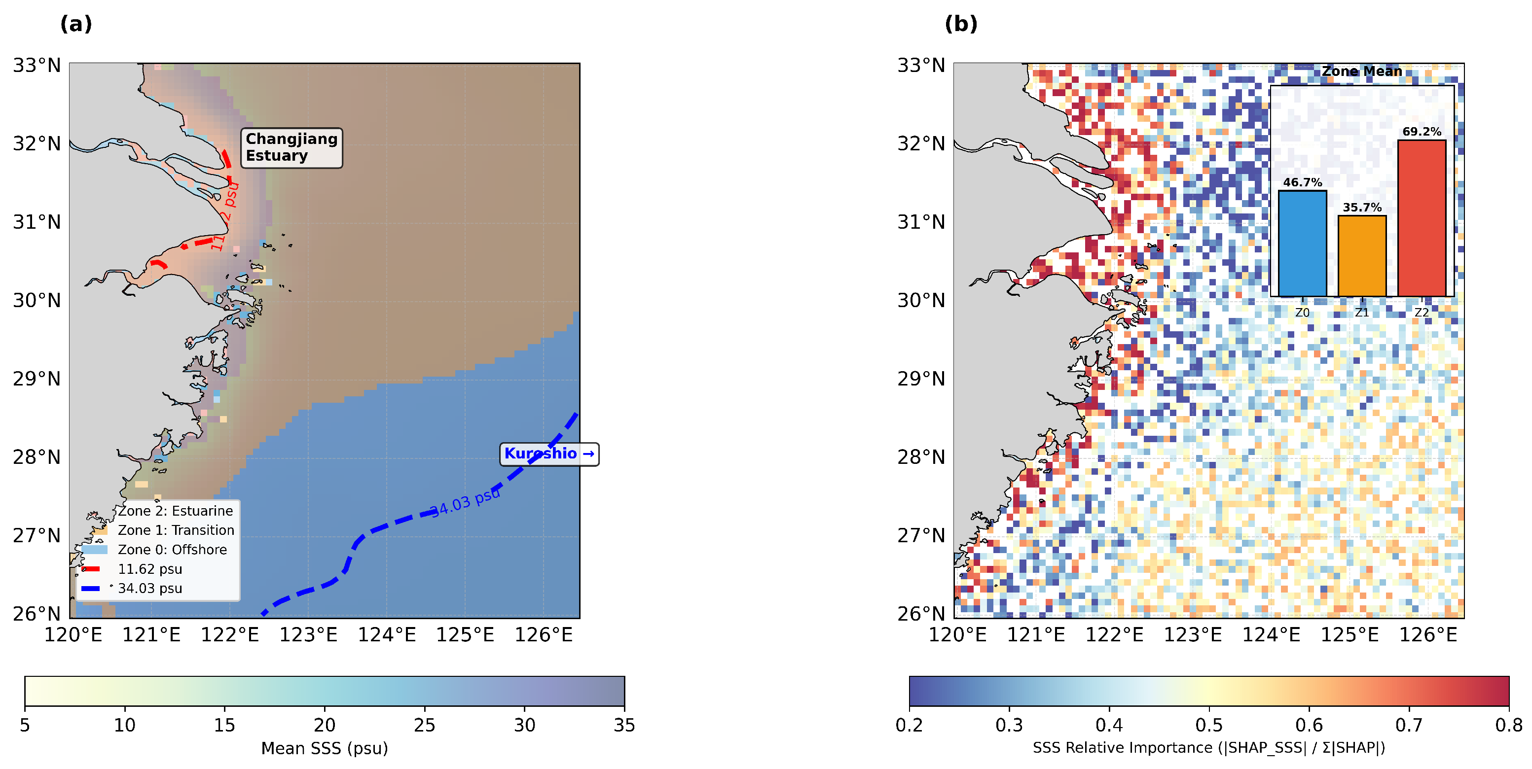
This triple-role transition is quantitatively confirmed by the directional SHAP analysis (Figure 8b), which shows mean SSS SHAP values shifting from strongly positive in Zone 2 ($+1.026$) through weakly positive in Zone 1 ($+0.040$) to negative in Zone 0 ($-0.310$). Spatially, this corresponds to positive SHAP values (promoting Chl-a) dominating near-coast and estuarine waters, transitioning to negative SHAP values (inhibiting Chl-a) in offshore Kuroshio-influenced regions, with the zone boundary contours at 11.62 and 34.03 psu delineating the mechanistic transitions (see also Figure 6c for spatial regime mapping). This framework resolves the apparent contradiction of SSS being both the dominant positive and negative driver: it is not the salinity value per se but the ecological processes SSS proxies that change across the gradient.

4.4. Hierarchical Control and Climate Change Implications

The 97.4% SSS versus 2.6% PAR attribution in estuarine waters (renormalized SSS–PAR pair; Section 3.4) challenges light-limitation paradigms: while PAR mechanistically limits productivity, salinity-mediated turbidity governs variance. This hierarchical structure—where SSS acts as a “gatekeeper” integrating flocculation, turbidity, nutrients, residence time, and frontal dynamics—explains weak Chl-a–PAR correlations commonly observed in field studies. The PAR SHAP dependence analysis (Figure 5c) confirmed that light effects are uniformly weak across all zones, supporting SSS as the master environmental proxy.

We note that the ecological effect of a given PAR level is inherently season-dependent: for instance, a particular irradiance may be sufficient for phytoplankton growth in winter (when community metabolic demands are lower) but insufficient in spring (when bloom-forming diatoms require higher photon fluxes). Because the model uses monthly-averaged surface PAR—which cannot capture such context-dependent light thresholds—it is unsurprising that SSS, which integrates information about the underwater light environment through its correlation with turbidity, emerges as the more informative predictor. This does not imply that light is ecologically unimportant but rather that at the spatiotemporal scales of this analysis, SSS encodes the relevant light information more effectively than surface PAR.

The 61% modulation of SST effects by nutrient status (Table 7) has direct climate implications. Traditional additive models assuming uniform warming effects will systematically err: temperature-driven productivity gains are approximately 2.5 times larger in nutrient-rich versus nutrient-poor waters. Furthermore, Kuroshio intensification under climate change [28,39] may expand the “dilution paradox” regime where warming combined with oligotrophy reduces productivity, a pattern potentially exacerbated by evolving ENSO dynamics [40,41].

The seasonal modulation revealed by Figure 8a provides additional nuance: estuarine SSS effects are slightly stronger in winter ($S/W=0.9\times$), consistent with winter peak sediment discharge, while offshore effects show minimal seasonal variation, reflecting the relatively stable Kuroshio influence.

4.5. Applications for Ecosystem Monitoring

The identified thresholds enable operational satellite-based monitoring: SSS crossing 11.62 psu anticipates 93% Chl-a increase; crossing 34 psu signals oligotrophic transition. The SST × ZOS interaction—2.6-fold overall amplification, reaching ∼7-fold under warm-water conditions (SST $>{27 }^{\circ }$C)—provides a satellite-detectable indicator for Kuroshio intrusion events affecting offshore fisheries. Zone-specific driver hierarchies guide management: sediment control for estuarine zones, nutrient reduction for transitional zones, and Kuroshio forecasting for offshore areas.

The SSS Triple-Role Framework (Figure 8) provides a unifying conceptual model for interpreting satellite-derived salinity patterns in river-dominated marginal seas globally, with potential application to the Amazon Plume, Ganges–Brahmaputra Delta, and Mississippi River systems.

4.6. Limitations and Future Directions

Key limitations are as follows: (1) CMEMS SSS is a reanalysis product whose effective spatial resolution may be coarser than the nominal 0.083° grid due to data assimilation smoothing, potentially underrepresenting sub-mesoscale salinity fronts. (2) MODIS-Aqua PAR, as a satellite-derived composited product, is subject to cloud contamination that is particularly severe in the ECS during the mei-yu (plum rain) season, potentially smoothing out ecologically relevant short-term light variability; unlike the reanalysis-based SST, SSS, and ZOS fields which provide gap-free coverage through data assimilation, the PAR product retains observational gaps that monthly compositing may not fully resolve—this data quality asymmetry could partially contribute to the low PAR attribution (1.9–4.4%), though the physical argument that SSS proxies the underwater light field more effectively than surface PAR in turbid waters remains the primary explanation. (3) SSS–nutrient correlation weakens with sewage discharge. (4) The temporal split places the extreme 2020 Changjiang flood in the test period, which deliberately tests robustness under unprecedented conditions but may yield conservative performance estimates compared to a test set spanning only non-extreme years. (5) Both zone delineation (K-means on SSS) and threshold detection (SHAP gradients on SSS) share dependence on salinity as the primary signal. Although the two methods are independent (unsupervised clustering versus supervised attribution) and the detected thresholds (11.62 and 34.03 psu) do not coincide with K-means zone boundaries (∼28 and ∼32 psu), we encourage future validation using alternative zonation criteria such as bathymetric contours or T-S diagram–based water mass classification [42]. (6) SHAP analysis was performed on a stratified subsample of 5000 observations (0.35% of the full dataset); while convergence tests confirmed consistent results across sample sizes from 1000 to 20,000 (Section 2.5), future studies employing GPU-accelerated SHAP implementations could enable full-dataset attribution, potentially refining threshold precision in data-sparse regimes. (7) The counterfactual experiments tested model-learned associations under perturbation rather than true causal interventions—unmeasured confounders or nonlinear feedbacks not captured in the training data could alter real-world responses, and the results should therefore be interpreted as evidence of learned environmental sensitivity rather than strict causation. (8) Unequal data volumes across zones may affect statistical power: the SHAP subsample ($n=5000$) preserves original zone proportions, meaning offshore observations dominate, while there are fewer estuarine observations—this reflects the genuine spatial distribution but implies that zone-specific interaction analyses with additional conditioning (e.g., SST × ZOS in Zone 0 for SST $>{27 }^{\circ }$C, where $n=21$ in the SHAP subsample) have limited statistical power and should be interpreted with caution. Bootstrap confidence intervals partially address this, but future studies should consider zone-stratified oversampling strategies for interaction analyses. Future work should integrate NASA PACE hyperspectral data, apply CMIP6 projections under the hierarchical control framework, and validate thresholds in other river-dominated systems (Amazon, Ganges–Brahmaputra, and Mississippi). Additionally, future studies comparing the geography-free approach with spatiotemporal feature integration strategies could further clarify the tradeoff between predictive accuracy and mechanistic interpretability.

5. Conclusions

Integrating 22 years of multi-source satellite data with SHAP attribution revealed four major findings for East China Sea Chl-a dynamics:

(1) Dual thresholds: 11.62 psu ($d=-2.92$) marks the turbidity-to-productivity transition; 34.03 psu ($d=-1.04$) extends the ecological CDW boundary 20,000 ${\mathrm{km}}^2$ beyond physical definitions.

(2) SSS Triple-Role Framework: SSS plays three mechanistically distinct roles—turbidity proxy (estuarine, SHAP $=+1.026$), nutrient proxy (transition, SHAP $=+0.040$), and dilution signal (offshore, SHAP $=-0.310$)—resolving the apparent contradiction of simultaneous positive and negative salinity effects.

(3) Non-additive interactions: SSS × SST coupling (61% modulation) and SST × ZOS Kuroshio detection (2.6-fold overall, ∼7-fold under warm-water conditions) demonstrate hierarchical control missed by additive models.

(4) Geography-free interpretability: Although the +Location model achieved higher overall accuracy ($R^2=0.954$ versus 0.802), counterfactual experiments revealed it retains only 4.6% environmental sensitivity in the flood-critical estuarine zone (34.3% overall). Multi-scenario validation across four distinct perturbation types (SSS, SST, and ZOS) confirmed this pattern, with the +Location model retaining only 29% sensitivity on average, confirming that geography-free design is essential for counterfactual-based mechanistic attribution and climate change applicability.

This satellite–AI framework provides quantitative benchmarks for ecosystem monitoring in river-dominated marginal seas globally.

References

1. Behrenfeld, M.J.; O’Malley, R.T.; Siegel, D.A.; McClain, C.R.; Sarmiento, J.L.; Feldman, G.C.; Milligan, A.J.; Falkowski, P.G.; Letelier, R.M.; Boss, E.S. Climate-driven trends in contemporary ocean productivity. Nature 2006, 444, 752–755. [Google Scholar] [CrossRef] [Scilit] [PubMed]
2. Zhou, Z.X.; Yu, R.C.; Zhou, M.J. Resolving the complex relationship between harmful algal blooms and environmental factors in the coastal waters adjacent to the Changjiang River estuary. Harmful Algae 2017, 62, 60–72. [Google Scholar] [CrossRef] [Scilit]
3. Chen, C.C.; Shiah, F.K.; Gong, G.C.; Chen, T.Y. Impact of upwelling on phytoplankton blooms and hypoxia along the Chinese coast in the East China Sea. Mar. Pollut. Bull. 2021, 167, 112288. [Google Scholar] [CrossRef] [Scilit] [PubMed]
4. Zhou, M.J.; Shen, Z.L.; Yu, R.C. Responses of a coastal phytoplankton community to increased nutrient input from the Changjiang (Yangtze) River. Cont. Shelf Res. 2008, 28, 1483–1489. [Google Scholar] [CrossRef] [Scilit]
5. Bai, Y.; He, X.; Pan, D.; Chen, C.T.A.; Kang, Y.; Chen, X.; Cai, W.J. Summertime Changjiang River plume variation during 1998–2010. J. Geophys. Res. Ocean. 2014, 119, 6238–6257. [Google Scholar] [CrossRef] [Scilit]
6. Siswanto, E.; Tang, J.; Yamaguchi, H.; Ahn, Y.H.; Ishizaka, J.; Yoo, S.; Kim, S.W.; Kiyomoto, Y.; Yamada, K.; Chiang, C.; et al. Empirical ocean-color algorithms to retrieve chlorophyll-a, total suspended matter, and colored dissolved organic matter absorption coefficient in the Yellow and East China Seas. J. Oceanogr. 2011, 67, 627–650. [Google Scholar] [CrossRef] [Scilit]
7. Gong, G.C.; Wen, Y.H.; Wang, B.W.; Liu, G.J. Seasonal variation of chlorophyll a concentration, primary production and environmental conditions in the subtropical East China Sea. Deep-Sea Res. Part II Top. Stud. Oceanogr. 2003, 50, 1219–1236. [Google Scholar] [CrossRef] [Scilit]
8. Lie, H.J.; Cho, C.H. Seasonal circulation patterns of the Yellow and East China Seas derived from satellite-tracked drifter trajectories and hydrographic observations. Prog. Oceanogr. 2016, 146, 121–141. [Google Scholar] [CrossRef] [Scilit]
9. Zhu, Z.Y.; Zhang, J.; Wu, Y.; Zhang, Y.Y.; Lin, J.; Liu, S.M. Hypoxia off the Changjiang (Yangtze River) Estuary: Oxygen depletion and organic matter decomposition. Mar. Chem. 2011, 125, 108–116. [Google Scholar] [CrossRef] [Scilit]
10. Chen, C.T.A. Chemical and physical fronts in the Bohai, Yellow and East China seas. J. Mar. Syst. 2009, 78, 394–410. [Google Scholar] [CrossRef] [Scilit]
11. Hu, C.; Lee, Z.; Franz, B. Chlorophyll-a algorithms for oligotrophic oceans: A novel approach based on three-band reflectance difference. J. Geophys. Res. Ocean. 2012, 117, C01011. [Google Scholar] [CrossRef] [Scilit]
12. Wu, H.; Shen, J.; Zhu, J.; Zhang, J.; Li, L. Characteristics of the Changjiang plume and its extension along the coast of the East China Sea. Cont. Shelf Res. 2019, 183, 33–48. [Google Scholar] [CrossRef] [Scilit]
13. Cloern, J.E. Turbidity as a control on phytoplankton biomass and productivity in estuaries. Cont. Shelf Res. 1987, 7, 1367–1381. [Google Scholar] [CrossRef] [Scilit]
14. Sauzeède, R.; Bittig, H.C.; Claustre, H.; Pasqueron de Fommervault, O.; Gattuso, J.P.; Legendre, L.; Johnson, K.S. Estimates of water-column nutrient concentrations and carbonate system parameters in the global ocean: A novel approach based on neural networks. Front. Mar. Sci. 2016, 3, 128. [Google Scholar] [CrossRef] [Scilit]
15. Blix, K.; Pálffy, K.; Tóth, V.R.; Eltoft, T. Remote sensing of water quality parameters over Lake Balaton by using Sentinel-2 and Sentinel-3. Water 2018, 10, 1428. [Google Scholar] [CrossRef] [Scilit]
16. Lundberg, S.M.; Lee, S.I. A unified approach to interpreting model predictions. In Proceedings of the Advances in Neural Information Processing Systems 30 (NeurIPS 2017); Curran Associates, Inc.: Red Hook, NY, USA, 2017; pp. 4765–4774. [Google Scholar]
17. Mamalakis, A.; Ebert-Uphoff, I.; Barnes, E.A. Neural network attribution methods for problems in geoscience: A novel synthetic benchmark dataset. Environ. Data Sci. 2022, 1, e8. [Google Scholar] [CrossRef] [Scilit]
18. Mattei, F.; Scardi, M. Embedding ecological knowledge in machine learning to map spatial distributions of chlorophyll-a in the Mediterranean Sea. Ecol. Inform. 2024, 79, 102424. [Google Scholar] [CrossRef] [Scilit]
19. Luo, Y.; Zhao, T.; Mao, J.; Shi, J. Explainable AI for environmental science: A review. Artif. Intell. Rev. 2023, 56, 13473–13527. [Google Scholar]
20. El Hourany, R.; Pierella Karlusich, J.J.; Zinger, L.; Loisel, H.; Levy, M.; Bowler, C. Linking satellites to genes with machine learning to estimate phytoplankton community structure from space. Ocean. Sci. 2024, 20, 217–239. [Google Scholar] [CrossRef] [Scilit]
21. Han, J.W.; Kim, T.; Lee, S.; Kang, T.; Im, J.K. Machine learning and explainable AI for chlorophyll-a prediction in Namhan River Watershed, South Korea. Ecol. Indic. 2024, 166, 112361. [Google Scholar] [CrossRef] [Scilit]
22. Kruk, M. Prediction of environmental factors responsible for chlorophyll a-induced hypereutrophy using explainable machine learning. Ecol. Inform. 2023, 75, 102047. [Google Scholar] [CrossRef] [Scilit]
23. Kim, H.C.; Yamaguchi, H.; Yoo, S.; Zhu, J.; Okamura, K.; Kiyomoto, Y.; Tanaka, K.; Kim, S.-W.; Park, T.; Oh, I.S.; et al. Distribution of Changjiang Diluted Water detected by satellite chlorophyll-a and its interannual variation during 1998–2007. J. Oceanogr. 2009, 65, 129–135. [Google Scholar] [CrossRef] [Scilit]
24. Chen, T.; Guestrin, C. XGBoost: A Scalable Tree Boosting System. In Proceedings of the 22nd ACM SIGKDD International Conference on Knowledge Discovery and Data Mining; ACM: New York, NY, USA, 2016; pp. 785–794. [Google Scholar] [CrossRef] [Scilit]
25. Georganos, S.; Grippa, T.; Vanhuysse, S.; Lennert, M.; Shimoni, M.; Wolff, E. Very high resolution object-based land use–land cover urban classification using extreme gradient boosting. IEEE Geosci. Remote Sens. Lett. 2018, 15, 607–611. [Google Scholar] [CrossRef] [Scilit]
26. Zhou, X.; Ge, J.; Wallhead, P.; Shi, S. Contrasting impacts of flooding and tropical cyclones on estuarine plume environments. Limnol. Oceanogr. 2025, 70, e10152. [Google Scholar] [CrossRef] [Scilit]
27. Lundberg, S.M.; Erion, G.; Chen, H.; DeGrave, A.; Prutkin, J.M.; Nair, B.; Katz, R.; Himmelfarb, J.; Bansal, N.; Lee, S.I. From local explanations to global understanding with explainable AI for trees. Nat. Mach. Intell. 2020, 2, 56–67. [Google Scholar] [CrossRef] [Scilit] [PubMed]
28. Lee, D.G.; Oh, J.H.; Noh, K.M.; Kwon, E.Y.; Kim, Y.H.; Kug, J.S. What controls the future phytoplankton change over the Yellow and East China Seas under global warming? Front. Mar. Sci. 2023, 10, 1010341. [Google Scholar] [CrossRef] [Scilit]
29. Tseng, Y.H.; Shen, M.L.; Jan, S.; Dietrich, D.E.; Chiang, C.P. Validation of the Kuroshio current system in the dual-domain Pacific Ocean model framework. Prog. Oceanogr. 2014, 123, 30–43. [Google Scholar] [CrossRef] [Scilit]
30. Dijkstra, Y.M.; Schuttelaars, H.M.; Schramkowski, G.P.; Brouwer, R.L. Modeling the transition to high sediment concentrations as a response to channel deepening in the Ems River Estuary. J. Geophys. Res. Ocean. 2019, 124, 1578–1594. [Google Scholar] [CrossRef] [Scilit]
31. Li, W.; Ge, J.; Ding, P.X.; Ma, J.; Glibert, P.M.; Liu, D. Effects of dual fronts on the spatial pattern of chlorophyll-a concentrations in and off the Changjiang River Estuary. Estuaries Coasts 2021, 44, 1–11. [Google Scholar] [CrossRef] [Scilit]
32. Asmala, E.; Bowers, D.G.; Autio, R.; Kaartokallio, H.; Thomas, D.N. Qualitative changes of riverine dissolved organic matter at low salinities due to flocculation. J. Geophys. Res. Biogeosci. 2014, 119, 1919–1933. [Google Scholar] [CrossRef] [Scilit]
33. Bianchi, T.S.; Allison, M.A. Large-river delta-front estuaries as natural “recorders” of global environmental change. Proc. Natl. Acad. Sci. USA 2010, 107, 8685–8690. [Google Scholar] [CrossRef] [Scilit] [PubMed]
34. Wang, B.D.; Chen, J.F.; Jin, H.Y.; Li, H.L.; Huang, D.J.; Cai, W.J. Diatom bloom-derived bottom water hypoxia off the Changjiang estuary, with and without typhoon influence. Limnol. Oceanogr. 2014, 59, 1679–1689. [Google Scholar] [CrossRef] [Scilit]
35. Jiang, Z.; Liu, J.; Chen, J.; Chen, Q.; Yan, X.; Xuan, J.; Zeng, J. Responses of summer phytoplankton community to drastic environmental changes in the Changjiang (Yangtze River) Estuary during the past 50 years. Water Res. 2014, 54, 1–11. [Google Scholar] [CrossRef] [Scilit]
36. Kwon, H.K.; Kim, G.; Hwang, J.; Lim, W.A.; Park, J.W.; Kim, T.H. Significant and conservative long-range transport of dissolved organic nutrients in the Changjiang diluted water. Sci. Rep. 2018, 8, 12693. [Google Scholar] [CrossRef] [Scilit]
37. Wei, Q.; Wang, B.; Zhang, X.; Ran, X.; Fu, M.; Sun, X.; Yu, Z. Contribution of the offshore detached Changjiang (Yangtze River) Diluted Water to the formation of hypoxia in summer. Sci. Total Environ. 2021, 764, 142838. [Google Scholar] [CrossRef] [Scilit] [PubMed]
38. Sun, Q.; Li, D.; Wang, B.; Xu, Z.; Miao, Y.; Lin, H.; Jin, H.; Jiang, Z.; Zeng, J.; Zhou, F.; et al. Massive nutrients offshore transport off the Changjiang Estuary in flooding summer of 2020. Front. Mar. Sci. 2023, 10, 1076336. [Google Scholar] [CrossRef] [Scilit]
39. Jang, C.J.; Park, J.; Park, T.; Yoo, S. Response of the ocean mixed layer depth to global warming and its impact on primary production: A case for the North Pacific Ocean. ICES J. Mar. Sci. 2011, 68, 996–1007. [Google Scholar] [CrossRef] [Scilit]
40. Cai, W.; Santoso, A.; Collins, M.; Dewitte, B.; Karamperidou, C.; Kug, J.S.; Lengaigne, M.; McPhaden, M.J.; Stuecker, M.F.; Taschetto, A.S.; et al. Changing El Niño–Southern Oscillation in a warming climate. Nat. Rev. Earth Environ. 2021, 2, 628–644. [Google Scholar] [CrossRef] [Scilit]
41. Lee, D.G.; Oh, J.H.; Kam, J.; Kug, J.S. Phytoplankton blooming mechanisms over the East China Sea during post-El Niño summers. Biogeosciences 2025, 22, 3165–3180. [Google Scholar] [CrossRef] [Scilit]
42. Longhurst, A.R. Ecological Geography of the Sea, 2nd ed.; Academic Press: Burlington, MA, USA, 2007. [Google Scholar] [CrossRef] [Scilit]
Figure 1. Study area and data overview. (a) Oceanographic setting of the East China Sea showing the Changjiang Estuary, major current pathways, and study domain. (b) K-means zone classification with mean salinity background and dual salinity thresholds overlaid. Inset pie chart shows zone area proportions. (c) Multi-source satellite data temporal coverage, with the green-shaded region highlighting the common study period (2003–2024).
Remotesensing 18 01392 g001
Figure 2. Counterfactual flood experiment comparing the Environment-only (geography-free) and +Location models during the 2020 extreme event. All Δ Chl-a values are in original Chl-a space ( mg/m 3 ). (a) Factual Chl-a distribution (July 2020). (b) Δ Chl-a from the Environment-only model. (c) Δ Chl-a from the +Location model. (d) Feature-level sensitivity comparison. Scenario-level sensitivity ratios in ln ( 1 + Chl-a ) space are reported in Table 4.
Remotesensing 18 01392 g002
Figure 3. XGBoost versus SHAP feature importance comparison for Chl-a prediction. (a) Normalized importance scores from XGBoost gain (blue) and SHAP mean absolute values (red). (b) Correlation analysis between the two importance metrics, with dashed line indicating perfect correlation.
Remotesensing 18 01392 g003
Figure 4. Zone-specific SHAP attribution analysis. (a) Feature importance by zone. (b) SSS SHAP dependence across the full salinity gradient, colored by zone, with dual threshold annotations. (c) Driving force composition as stacked bars by zone. (d) Pixel-level spatial dominant driver map with inset pie chart.
Remotesensing 18 01392 g004
Figure 5. Environmental limitation regimes: SSS versus PAR across ecological zones. (a) Absolute SHAP importance for PAR and SSS with SSS:PAR ratios annotated. (b) Relative contributions as stacked bars showing SSS-mediated dominance across all zones. (c) PAR SHAP dependence by zone. (d) Spatial SSS:PAR importance ratio map with zone boundary contours.
Remotesensing 18 01392 g005
Figure 6. Dual salinity threshold validation and ecological regime classification. (a) SSS–SHAP dependence colored by season with regime backgrounds and dual threshold lines. (b) SHAP distribution by regime as box plots with effect sizes and sample sizes. (c) Spatial regime classification with area proportions and isohaline contours. *** p < 0.001.
Remotesensing 18 01392 g006
Figure 7. Multi-scale environmental interactions. (a) SSS SHAP grouped by SST categories in Zone 1 (Transition). (b) Interaction effect summary with bootstrap 95% CI. (c) SST × ZOS interaction in Zone 0 (Offshore): SST versus SST SHAP colored by ZOS, revealing a “hook pattern” under Kuroshio intrusion. Asterisks denote statistical significance (*** p < 0.001 ).
Remotesensing 18 01392 g007
Figure 8. Mechanistic synthesis: SSS Triple-Role Framework. (a) Seasonal modulation of SSS effects by zone. (b) Cross-zone SSS mechanism transition: directional SHAP values shifting from positive (Chl-a promotion) in estuarine waters to negative (Chl-a inhibition) offshore.
Remotesensing 18 01392 g008