Physics-Aware Hybrid CNN–Transformer Network for GNSS-R Sea Surface Wind Speed Estimation

Highlights

What are the main findings?

• The proposed Physics-Aware Hybrid CNN–Transformer Network (PA-HCTN) achieves a global RMSE of 1.35 m/s and an R² of 0.75 for sea surface wind speed estimation from CYGNSS data, outperforming existing deep learning benchmarks.
• The model significantly mitigates the high-wind-speed underestimation bias (reducing it to −3.90 m/s for winds > 15 m/s) by integrating a GMF-constrained loss function and a cross-attention mechanism for the dynamic fusion of auxiliary physical parameters.

What are the implications of the main findings?

• The work demonstrates the effectiveness of synergizing a CNN’s local feature extraction with a Transformer’s global context modeling, coupled with physics-guided fusion, providing a novel architecture paradigm for GNSS-R geophysical parameter retrieval.
• The successful integration of physical constraints into the deep learning framework enhances model robustness and physical consistency, offering a viable solution to improve the accuracy of extreme weather monitoring using spaceborne GNSS-R.

Abstract

Global Navigation Satellite System Reflectometry (GNSS-R) provides a promising approach for global ocean wind monitoring with high temporal resolution. However, accurate wind speed retrieval remains challenging due to the complex scattering mechanisms and the nonlinear coupling between delay–Doppler maps (DDMs) and observation geometries. To address these limitations, a Physics-Aware Hybrid CNN–Transformer Network (PA-HCTN) is proposed accordingly. The model integrates a CNN for local DDM feature extraction, a Transformer encoder for global context modeling, and a cross-attention module to dynamically fuse auxiliary physical parameters. A geophysical model function (GMF)-constrained loss is incorporated to enhance physical consistency. Evaluated on CYGNSS and ERA5 data, the PA-HCTN achieves an RMSE of 1.35 m/s and an R² of 0.75, outperforming existing benchmarks and significantly mitigating high-wind-speed underestimation. In addition, through independent validation using NDBC buoy data from four sites, the results demonstrate the effectiveness of the hybrid architecture and physics-aware design for GNSS-R wind retrieval.

1. Introduction

Sea surface wind speed (SSWS) is a core driving parameter in oceanography research and meteorological applications, holding great significance for studying global energy balance, ocean circulation, and air–sea interactions [1,2]. Traditional global wind observation methods primarily include in situ buoys, ship-based observations, and spaceborne remote sensing techniques like microwave scatterometers [3,4], radiometers, and Synthetic Aperture Radar (SAR). However, while buoy observations offer high accuracy, their spatial distribution is extremely sparse and maintenance is costly [5]. Some traditional satellite remote sensing techniques, such as Synthetic Aperture Radar (SAR), are often constrained by narrow swaths, while polar-orbiting radiometers and scatterometers, despite their wide swaths, typically have limited temporal resolution (long revisit times). This makes it difficult to capture the full lifecycle of rapidly evolving, small-scale meteorological events [6]. For coastal zones, high-frequency (HF) radar and X-band marine radar offer high-resolution wind mapping [7,8]. However, the limitations of these technologies in coastal areas have driven the development of GNSS-R technology on a global scale.

Global Navigation Satellite System Reflectometry (GNSS-R), as a bistatic radar remote sensing technology, utilizes existing navigation satellites in Earth orbit as signal sources to receive L-band signals reflected from the sea surface. It exhibits significant potential due to its low power consumption, low cost, high revisit rate, and all-weather monitoring capability [9,10]. GNSS-R technology offers an innovative, low-cost, weather-independent, and high-frequency monitoring pathway for achieving global wind observations [11]. Beyond wind speed retrieval, GNSS-R applications have expanded to various fields, including significant wave height retrieval [12], sea ice detection [13], sea ice type classification [14], and soil moisture monitoring [15]. Since the PARIS concept was proposed by Martin-Neira in 1993 [16], GNSS-R technology has undergone rapid iteration from ground-based, airborne to spaceborne experiments [17,18]. Early missions like UK-DMC and TechDemoSat-1 (TDS-1) successfully demonstrated the feasibility of detecting ocean features from space [19,20]. Subsequently, the NASA-launched Cyclone Global Navigation Satellite System (CYGNSS) constellation, comprising eight microsatellites, achieved high-frequency coverage of wind speeds in tropical regions, pushing GNSS-R towards operational application [21,22].

Table 1. Development history of spaceborne GNSS-R missions.

Mission Name	Launch Year	Agency	Orbit Feature	Primary Signal Source	Key Contribution
UK-DMC	2003	SSTL (UK)	Polar	GPS	First space-based validation
TDS-1	2014	SSTL (UK)	Polar	GPS	First publicly available large dataset
CYGNSS	2016	NASA (USA)	Tropical Low-Inclination	GPS	High revisit, typhoon monitoring
BuFeng-1	2019	CAST (China)	Low Earth Orbit	GPS, BeiDou	First detection of BeiDou reflected signals
FSSCat	2020	ESA (EU)	Polar	GPS, Galileo	CubeSat multi-element monitoring
FY-3E	2021	CMA (China)	Dawn–Dusk Orbit	GPS, BeiDou, Galileo	Multi-mode/multi-frequency, global operation
PRETTY	2023	ESA (EU)	Polar (SSO)	GPS, Galileo (L5/E5a)	The world’s first low-angle-of-incidence CubeSat
Tianmu-1 Constellation	2024	CASIC (China)	Polar	GPS, BeiDou, Galileo, GLONASS	The world’s largest GNSS-R constellation (22 satellites)
HydroGNSS	2025	ESA (EU)	Polar	GPS, Galileo	First dedicated dual-satellite GNSS-R mission for hydrometeorology

outlines the development history of the Space GNSS-R missions.

In the evolution of GNSS-R wind speed retrieval, the initial methodology centered on geophysical model functions (GMFs) derived from the Zavorotny–Voronovich (Z-V) scattering model [23]. They established empirical mapping relationships with wind speed by extracting key observable variables from the DDM [24]. Clarizia et al. developed the retrieval algorithm for the CYGNSS Level 2 sea surface wind speed data product based on a method described in 2014, proving the feasibility of using DDMs for ocean wind speed estimation [25]. However, GMF-based methods have significant limitations. Their dependence on a small number of feature parameters means they struggle to model the full complexity of the wind-scattering relationship. Additionally, their retrievals are sensitive to confounding influences from factors like viewing geometry, antenna characteristics, and sea surface temperature.

In recent years, data-driven machine learning (ML) and deep learning (DL) techniques have provided new avenues to address the nonlinear modeling challenges of GNSS-R [26]. Early studies tried methods like Multi-layer Perceptron (MLP) [27], Support Vector Regression (SVR) [28], and Random Forest [29], demonstrating superior prediction performance compared to traditional GMFs. Wang et al. analyzed variable importance by comparing the wind speed retrieval performance of seven machine learning methods on CYGNSS data [30]. Liu et al. effectively enhanced global retrieval robustness by constructing an FA-RDN hybrid neural network that integrated geometric features, instrument status, and spatial auxiliary information [31]. Heng et al. proposed the MF-ANN method, combining feature selection and outlier filtering modules to optimize ANN-based wind speed retrieval, reducing the RMSE by 29.08% compared to a single ANN [32]. With the success of convolutional neural networks (CNNs) in image processing, using CNNs to extract features from DDM images has become a mainstream approach, as demonstrated by the CYGNSSnet model, which significantly reduced the global average error [33]. Sequence modeling techniques like Long Short-Term Memory (LSTM) and Transformer have also provided new ideas for GNSS-R wind speed retrieval. In particular, for continuous observation data sequences, such models can effectively capture the spatiotemporal correlation characteristics between adjacent DDMs [34]. Since 2023, the Transformer architecture, native to Natural Language Processing (NLP), has begun to emerge in the GNSS-R field. Zhao et al. proposed Transformer-based GNSS-R wind speed retrieval, which can compute correlations between any two positions in the input sequence through self-attention mechanisms to capture global information, and learn discriminative features between different wind speeds through sequence-level attention mechanisms, specifically addressing the issue of scarce high-wind-speed samples and imbalanced data distribution [35]. Qiao et al. proposed a CNN–Transformer hybrid network, introducing a weighted MSE loss function to address data imbalance, achieving RMSEs of 1.417 m/s for ECMWF data and 1.620 m/s for NDBC buoy data. A substantial gain was observed for high wind speeds (>15 m/s), where the RMSE was reduced by 20.3% [36]. Du et al. proposed a Deep Residual Fully Connected Network (RFCN), which effectively mitigates the degradation issues in deep networks by incorporating residual connections and multidimensional auxiliary information such as ocean current velocity. This approach significantly improves inversion accuracy at low to moderate wind speeds and explains the model’s physical mechanisms using SHAP theory [37]. In another study, Xu et al. addressed the limitations of traditional CNNs—namely, their limited receptive fields and difficulty in capturing global features of delayed Doppler maps (DDMs)—by proposing a dual-path network (WsCBAM) based on convolutional block attention modules. This approach enhances the model’s ability to fuse features from effective scattering regions and auxiliary parameters, thereby improving the accuracy and robustness of global wind speed inversion [38].

Although machine learning methods have greatly addressed the problems of low accuracy in traditional GNSS-R wind speed retrieval, existing models still face several challenges: On one hand, the inherent inductive bias of traditional CNNs limits their ability to capture long-range pixel correlations in DDM images, and their limited receptive field poses a challenge for capturing long-range dependencies within DDMs. While Transformer’s global self-attention mechanism excels at capturing long-distance dependencies, it lacks inductive bias for extracting local features. DDM images exhibit a significant physical structure, with primary energy concentrated near the specular reflection point and possessing a specific shape. The Transformer structure overlooks the strong correlation between adjacent pixels [34]. On the other hand, due to the scarcity of extreme wind speed samples, deep learning models often exhibit significant underestimation in the high-wind-speed range (>15 m/s). A common practice is to introduce auxiliary parameters such as GNSS-R signal and system data into the model. However, current multimodal fusion methods often only perform simple concatenation. This fusion strategy prevents image features and physical parameters from interacting throughout the feature extraction process. In reality, certain physical parameters greatly influence the DDM shape and amplitude. Simple concatenation causes the network to process DDMs without awareness of physical auxiliary information, potentially hindering its correct understanding of the physical meaning behind DDM shapes.

To address these issues, this paper proposes a Physics-Aware Hybrid CNN–Transformer Network. The architecture consists of three core components: (1) a CNN backbone for extracting local textures and scattering features from multi-channel DDMs; (2) a Transformer encoder for capturing long-range dependencies in the delay–Doppler domain; and (3) a cross-attention-based fusion module that dynamically integrates physical parameters into the DDM feature space. Unlike simple concatenation, this mechanism uses image features as queries and physical scalars as keys/values, guiding the model to focus on wind-sensitive regions under different conditions. Additionally, a GMF-based physical constraint loss term is introduced during training to enhance consistency between learned representations and theoretical scattering models, improving retrieval robustness under high-wind-speed conditions. This work aims to combine a CNN’s local feature extraction capability with Transformer’s global context modeling, together with multimodal fusion and physical constraints, to break through the accuracy limitations of existing methods.

The structure of the remaining sections is as follows: Section 2 describes the dataset and quality control procedures; Section 3 details the PA-HCTN architecture and training methodology; Section 4 presents the experimental setup and results analysis; and Section 5 concludes the paper and suggests directions for future research.

2. Data

2.1. Data Sources

(1) CYGNSS: This study uses the CYGNSS Level 1 Version 3.1 dataset [39], a standardized scientific product from NASA’s Cyclone Global Navigation Satellite System mission. The data used in this work cover the entire year of 2024. The CYGNSS constellation provides measurements over the latitude range of approximately ± 38°, which covers the majority of tropical cyclone formation and evolution regions. The Level 1 data processing involves rigorous steps including raw data decoding, instrument calibration, geometric positioning, and the generation of standardized geophysical observables, with the DDM as the core data entity. Furthermore, 14 auxiliary parameters covering signal characteristics and geometric dynamics are selected from this dataset, as detailed in

Table 2. List of ancillary parameters.

Input Parameters		Descriptions	Potential Value
Signal Characteristics	ddm_nbrcs	Normalized Bistatic Radar Cross Section	Affects the Doppler–delay output
	ddm_les	Slope of the leading edge of the DDM waveform
	ddm_snr	SNR of the leading edge of the DDM waveform	Signal strength and reliability related
	sp_rx_gain	Antenna gain of the receiver in the direction of the specular reflection point	Affects reflected signal DDM power waveform
	gps_eirp	GPS Effective Isotropic Radiated Power	System bias correction
Geometric Dynamics	sp_inc_angle	Angle of incidence at the specular reflection point	Affects how the signal interacts with the reflector
	rx_to_sp_range	Distance from receiver constellation to the specular reflection point	Affects signal power and delay
	tx_to_sp_range	Distance from transmitter constellation to the specular reflection point
	sc_vel_x, sc_vel_y, sc_vel_z	Receiver constellation velocities in the X, Y, and Z directions	Affects the Doppler–delay output
	tx_vel_x, tx_vel_y, tx_vel_z	Transmitter constellation velocities in the X, Y, and Z directions

.

The selection of the 14 ancillary parameters listed in Table 2 is guided by three primary considerations. Firstly, from a physical perspective, these parameters are known to directly influence the characteristics of DDMs and the reflected signal power. Secondly, prior studies on GNSS-R wind speed retrieval have widely adopted these variables as inputs to both geophysical model functions and machine learning models, demonstrating their effectiveness in reducing retrieval bias and capturing observational geometry effects. Thirdly, all selected parameters are operationally available from the CYGNSS Level 1 dataset, ensuring the reproducibility and applicability of the proposed model. By incorporating this comprehensive set of signal characteristics and geometric dynamics, the model is expected to better decouple the complex interactions between sea surface roughness and observation conditions.

(2) ERA5: The reference data come from the European Centre for Medium-Range Weather Forecasts’ fifth-generation reanalysis (ERA5) data [40]. ERA5 is generated by the ECMWF’s advanced Integrated Forecasting System (IFS Cy41r2), which dynamically assimilates vast amounts of heterogeneous global observational system data spanning decades into a numerical model, producing a physically consistent, spatiotemporally complete optimal estimation dataset describing multiple Earth system state variables. This study uses the ERA5 sea surface 10 m wind speed, including zonal (U₁₀) and meridional (V₁₀) components. With an hourly temporal resolution and a 0.25° × 0.25° horizontal grid, it captures the evolution of wind processes more finely. This study utilized data from the entire year of 2024, The period from 1 January to 30 June constitutes the training set, while 1 July to 31 August forms the validation set. The remaining data are used for testing.

(3) NDBC Buoy Data: To further validate the performance of the proposed model against independent in situ measurements, data from the National Data Buoy Center (NDBC) are utilized. Four buoy stations, namely 41002, 41049, 42060, and 51000, are selected based on data availability and their location covering different ocean regions and wind regimes during the test period. The buoy wind speeds, originally measured at various anemometer heights, are adjusted to the standard 10 m reference level using a power-law wind profile to ensure consistency with the model output and ERA5 references. A spatiotemporal matching window of 15 min and 0.25° is applied to collocate CYGNSS observations with buoy measurements. These data are available at https://www.ndbc.noaa.gov/historical_data.shtml (accessed on 14 March 2026).

2.2. Data Preparation

(1) Quality Control: Due to the long propagation distances inherent in spaceborne measurements, hardware limitations, and complex ocean dynamics, raw CYGNSS data contain many samples with extremely weak signals, nearly drowned out by thermal noise. To ensure the correctness and reliability of the dataset used, the following quality control is applied to the CYGNSS data:

• Quality flag filtering is performed. Data from “open ocean” are ensured, excluding land or near-land data.
• Data points missing key information are removed. If any of the selected features contains NaN for a given timestamp, that data point is discarded.
• Data with RCG < 3 or LES < 0 are removed. This typically effectively removes data at the antenna beam edge or with a very poor SNR.

$$\mathrm{RCG}={\displaystyle \frac{G_{\mathrm{sp}}^R\times {10}^{27}}{{(R_T^{\mathrm{sp}}{R}_R^{\mathrm{sp}})}^2}}$$

(1)

where $G_{\mathrm{sp}}^R$ is the receiver antenna gain, and $R_T^{\mathrm{sp}}$ and $R_R^{\mathrm{sp}}$ are the transmitter and receiver ranges to the specular point, respectively.

4.

Only data with the nanosat tracking status flag ‘0’ (indicating good status) are retained.

5.

Data with a signal-to-noise ratio < 3 or receiver antenna gain towards SP < 0 are removed.

It is worth noting that the quality control criterion of SNR ≥ 3, while effective in excluding noise-contaminated measurements, inevitably leads to a reduction in the number of valid samples under high-wind-speed conditions. This may introduce sampling bias, thereby hindering the model’s ability to learn true scattering behavior under extreme wind conditions. To mitigate this issue, the proposed PA-HCTN incorporates a GMF-constrained loss function and a cross-attention mechanism to enhance the utilization of auxiliary physical parameters, thereby improving retrieval robustness despite the limited availability of high-wind SNR observations.

(2) Data Labeling: Firstly, the final scalar wind speed is derived by synthesizing the ERA5 zonal ($U_{10}$) and meridional ($V_{10}$) components via Equation (2). Subsequently, spatial bilinear interpolation and temporal linear interpolation are employed to collocate each sample with the corresponding ERA5 wind data. This process precisely maps the ERA5 grid data—characterized by coarser spatiotemporal resolution—onto the unstructured coordinates of the CyGNSS observation points. Finally, a masking operation excludes invalid values (NaNs) to establish a strict one-to-one correspondence between the feature data and the target labels.

$$S=\sqrt{{U_{10}}^2+{V_{10}}^2}$$

(2)

3. Methods

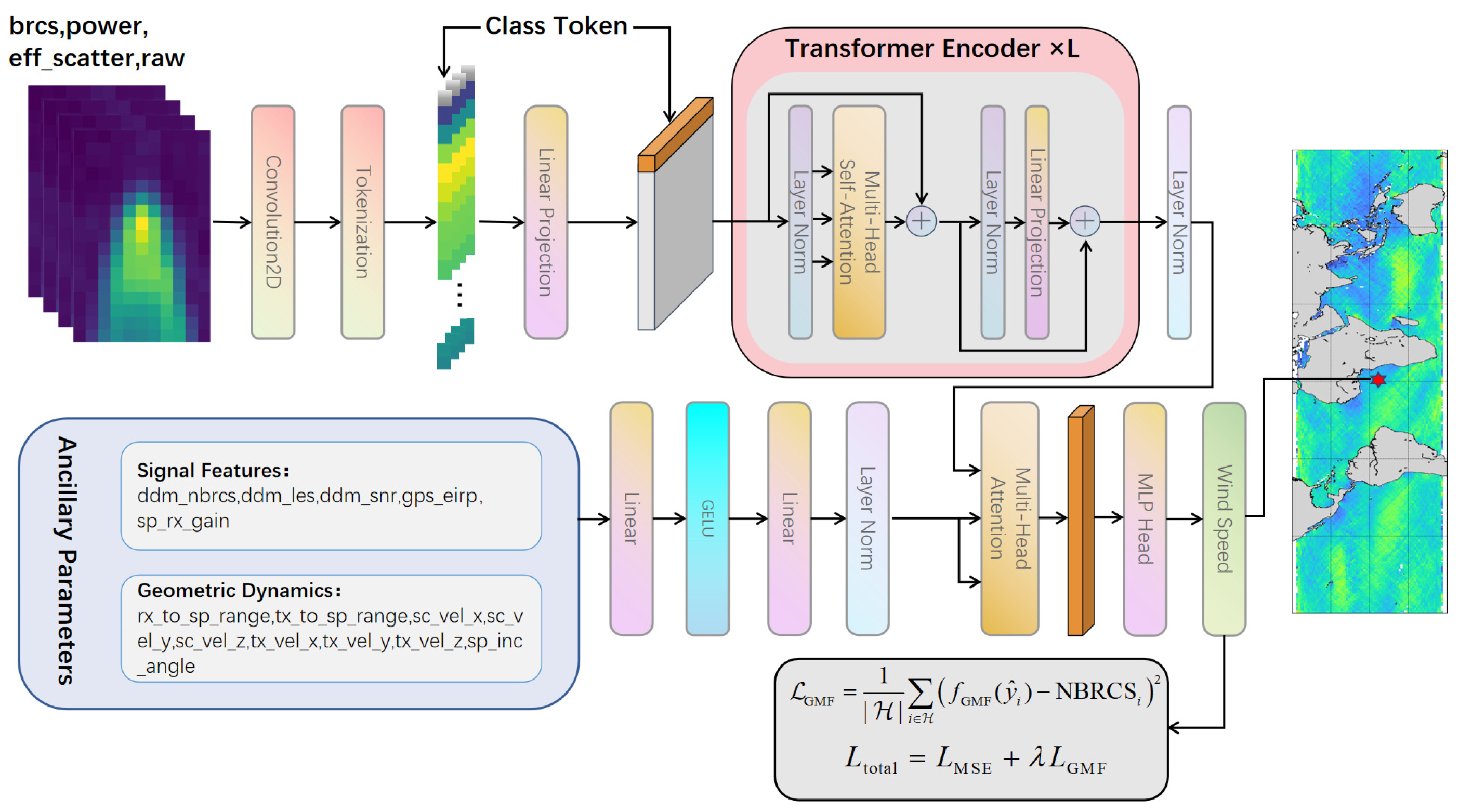
This section provides a detailed description of the PA-HCTN method. The model is designed to extract features from DDMs while incorporating multiple auxiliary features for wind speed retrieval. Figure 1 outlines the main structure of the model.

3.1. DDMs’ Feature Extraction Branch

This branch aims to extract deep spatiotemporal features from multi-channel DDMs. The overall architecture consists of three stages: CNN local feature extraction, serialization embedding with positional encoding, and global feature modeling based on a Transformer encoder.

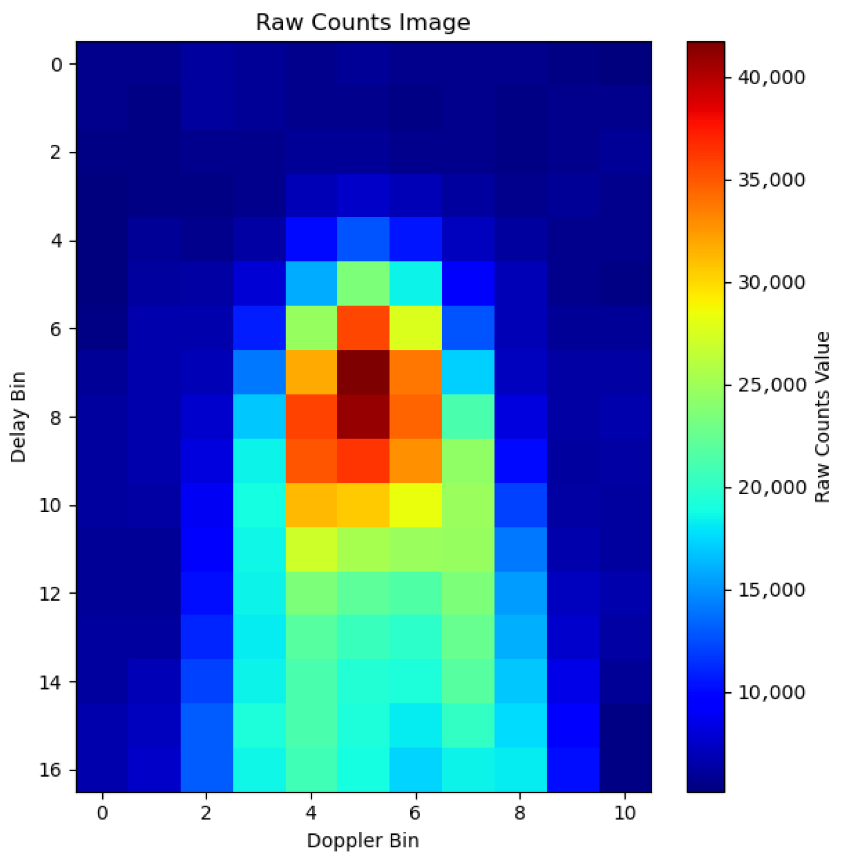
(1) CNN Local Feature Extraction: Considering the local spatial correlation of the physical “horseshoe” features present in DDM images (as shown in Figure 2), the model first encodes the raw input through a lightweight convolutional module. The input DDM data are represented as a tensor $X_{DDM}\in R^{B\times C_{\mathrm{i}n}\times H\times W}$, where $H=17,W=11$ are the spatial dimensions, and $C_{in}=4$ is the number of channels, corresponding to brcs, power, eff_scatter, raw_crds. To capture local correlations in the DDM image, a three-layer CNN module is designed, each with batch normalization and a ReLU activation function. The number of kernels is (16, 32, 32). Notably, DDMs are very small images. Using pooling layers would cause significant loss of spatial detail; therefore, pooling operations are omitted.

Let the CNN module be the mapping function $F_{cnn}(\cdot )$; its output feature map $F_{map}$ can be expressed as follows:

$$F_{map}=F_{cnn}(X_{DDM})\in R^{B\times C_{cnn}\times H\times W}$$

(3)

(2) Serialization and Class Token Embedding: To leverage the Transformer for processing global information, the 2D feature map must be converted into a sequence format. Firstly, $F_{map}$ is flattened along the spatial dimensions, obtaining the DDM pixel feature sequence $E_{pixels}\in R^{N\times C_{\mathrm{cnn}}}$, where $N=H\times W$. A learnable class token $E_{ct}\in R^{1\times C_{cnn}}$ is introduced to represent global information. This token is prepended to the DDM pixel sequence, forming the augmented sequence:

$$E_{seq}=[E_{ct};E_{pixels}]\in R^{(N+1)\times C_{cnn}}$$

(4)

Subsequently, a linear projection layer maps the feature dimension from $C_{cnn}$ to the Transformer’s hidden dimension $D$, and learnable positional encodings $P_{emb}$ are added to retain spatial positional information. The final embedded representation $E_0$ input to the encoder is as follows:

$$E_0=E_{seq}{W}_{proj}+P_{emb}$$

(5)

where $W_{proj}\in R^{C_{cnn}}\times D$ is the projection matrix, $E_0\in R^{(N+1)\times D}$.

(3) Transformer Encoder: This module is used to establish global contextual connections between the class token and all pixels. The module consists of $L$ stacked encoder layers, each containing layer normalization (LN), Multi-Head Self-Attention (MHSA), and a Feed-Forward Network (FFN).

Firstly, the input sequence $E_{l-1}$ undergoes layer normalization,

$$E_l^{\prime }=\mathrm{LA}(E_{l-1})$$

(6)

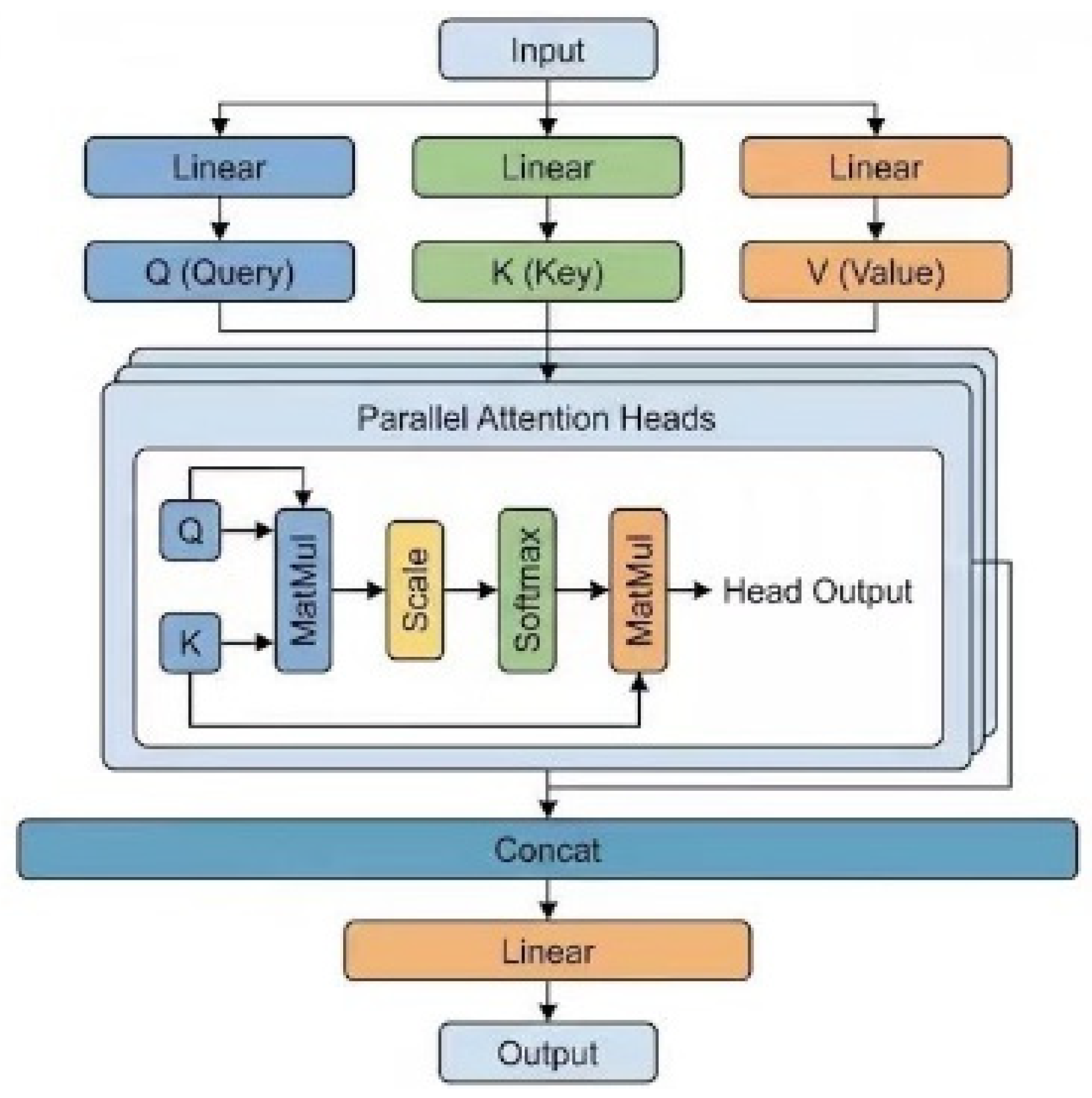
After LN, the MHSA mechanism establishes long-range dependencies within $E^{\prime }$. MHSA projects the input into queries (Q), keys (K), and values (V) using three learnable weight matrices $W^Q,W^K,W^V\in R^{D\times D}$. To enrich the feature subspace, the projected matrices are split along the feature dimension $D$ into $H$ heads, as shown in Figure 3. Mathematically, for the $i$-th head:

$$\begin{array}{l}Q=E_l^{\prime }{W}^Q=\{Q_1,Q_2,\dots ,Q_h\}\\ K=E_l^{\prime }{W}^K=\{K_1,K_2,\dots ,K_h\}\\ V=E_l^{\prime }{W}^V=\{V_1,V_2,\dots ,V_h\}\end{array}$$

(7)

where $Q_i,K_i,V_i\in R^{(N+1)\times (D/h)}$ represent the query, key, and value matrices for the $i$-th head respectively. Attention calculations are based on scaled dot products. The output of the $i$-th head is calculated as follows:

$$Hea{d}_i=Soft\max ({\displaystyle \frac{Q_i{K}_i^T}{\sqrt{d_k}}})V_i$$

(8)

The outputs of all heads are concatenated and fused via a linear transformation, followed by a residual connection, yielding the intermediate variable $Z_l$:

$$Z_l=E_{l-1}+Concat(Hea{d}_1,\dots ,Hea{d}_h)W^o$$

(9)

Finally, the features pass through a second LN layer and the FFN, outputting the final features $E_l$ for layer $l$:

$$E_l=Z_l+FFN(LA(Z_l))$$

(10)

After processing through $L$ layers, the feature vector at the first position of the sequence aggregates global information from the entire map and serves as the query vector for the subsequent cross-attention module.

3.2. Ancillary Parameters’ Feature Extraction Branch

The input data consist of 14 physical scalars. Z-Score normalization is first applied to eliminate scale effects and accelerate network convergence. To elevate the low-dimensional physical features to the same dimension $D$ as the image features, a nonlinear encoding module based on a Multi-Layer Perceptron (MLP) is constructed. This module comprises two fully connected layers, GELU activation, and layer normalization (LN).

$$H_{mid}=Dropout(GELU(S{W}_1+b_1)$$

(11)

$$S_{emb}=LA(H_{mid}{W}_2+b_2)$$

(12)

where $W_1\in R^{M\times D}$ and $b_1\in R^D$ are the weight matrix and bias term of the first layer, and $W_2\in R^{D\times D}$ and $b_2\in R^D$ are the parameters of the second layer.

3.3. Fusion Module

To effectively fuse the high-dimensional spatiotemporal features of DDM images with the physical environmental features of scalar data, the model designs a Multi-Head Cross-Attention module. This module breaks away from the simple linear superposition of features in traditional multimodal fusion, achieving pixel-level weighted enhancement of image features by physical features through asymmetric query–key–value mapping.

The fusion module receives feature inputs from two independent branches. Let the output from the image branch (Transformer encoder) be $E_{ing}\in R^{(N+1)\times D}$, where $N+1$ represents the sequence length (including the class token and pixel features). The output from the scalar branch (scalar encoder) is $E_{sca}\in R^{M\times D}$. $M$ represents the encoded global physical context vector. The cross-attention mechanism has a clear directionality: image features act as the “querier,” aiming to retrieve auxiliary information from scalar features. The query matrix $Q$ is generated solely from image features, while the key $K$ and value $V$ matrices are generated from scalar features. This process is expressed as follows:

$$Q=E_{img}{W}^Q, K=E_{sca}{W}^K, V=E_{sca}{W}^V$$

(13)

where $W^Q,W^K,W^V\in R^{D\times D}$ are learnable linear projection matrices. To capture semantic associations in different subspaces, the multi-head mechanism is similarly employed, splitting the above matrices into $h$ heads along the feature dimension.

The core of fusion lies in computing the correlation scores between image features and physical scalar features. For the $i$-th head, the attention weight matrix $A_i$ is calculated via the scaled dot product:

$$A_i=\mathrm{Softmax}\left({\displaystyle \frac{Q_i{K}_i^T}{\sqrt{d_k}}}\right)$$

(14)

Here, $A_i\in R^{(N+1)\times M}$ indicates the degree of attention each position in the image sequence pays to the physical scalar features. Subsequently, this weight is used to aggregate a weighted sum of the scalar feature values $V_i$, obtaining the feature representation $H_i$ fused with physical priors:

$$H_i=A_i{V}_i$$

(15)

The physical implication of this step lies in dynamically determining, based on the current texture state of the DDM image, how much information should be incorporated from the physical parameters, thereby refining the original DDM features.

The fused features are integrated via a linear layer $W^O$, and a residual connection is introduced. The final output $Z_{fused}{\in }^{(N+1)\times D}$ of the fusion module is mathematically expressed as follows:

$$Z_{fused}=\mathrm{LayerNorm}\left(E_{img}+\mathrm{Concat}(H_1,\dots ,H_h)W^O\right)$$

(16)

From the above formula, it can be seen that the output feature $Z_{fused}$ maintains the same sequence length and dimension as the input image feature $E_{img}$, but its internal representation is infused with physical environmental information injected via cross-attention. Finally, the model extracts only the first positional vector from this sequence for wind speed regression prediction.

Let the extracted feature vector be $Z_{final}\in R^D$. The regression head is designed as a three-layer MLP structure, aiming to achieve nonlinear mapping from the high-dimensional space to a one-dimensional variable.

$$\begin{array}{l}{h}_1=\mathrm{Dropout}(\mathrm{GELU}(z_{\mathrm{final}}{W}_i+b_1))\\ h_2=\mathrm{Dropout}(\mathrm{GELU}(h_1{W}_2+b_2))\\ \widehat{y}=h_2{W}_3+b_3\end{array}$$

(17)

3.4. Loss Function

Existing deep learning models primarily rely on the mean squared error (MSE) loss, defined as follows:

$$L_{MSE}={\displaystyle \frac{1}{N}}{\displaystyle \sum _{i=1}^n{(y_i-{\widehat{y}}_i)}^2}$$

(18)

where $N$ is the number of samples, and $y_i$ and ${\widehat{y}}_i$ represent the actual and estimated wind speed for the $i$-th sample, respectively.

To address the severe data imbalance, particularly the underrepresentation of samples with wind speeds > 15 m/s, models trained solely on the mean squared error tend to overfit in the low-to-medium speed range. Therefore, a physics-constrained composite loss function is adopted to ensure geophysically consistent wind speed estimations and enhance model robustness under high-wind conditions.

The adopted physical constraint is based on the GMF widely used in GNSS-R wind speed estimation. The relationship $f_{GMF}\left(u\right)$ can be piecewise expressed as follows:

$$NBRCS=f_{\mathrm{GMF}}\left(S\right)=\left\{\begin{array}{ll}{a}_0+a_1{S}^{-1}+a_2{S}^{-2},\hfill & S\le 15\mathrm{m}/\mathrm{s}\hfill \\ b_0+b_{1}S+b_2{S}^2,\hfill & S>15\mathrm{m}/\mathrm{s}\hfill \end{array}\right.$$

(19)

where $S$ denotes the wind speed, and $\{a_0,a_1,a_2\}$ and $\{b_0,b_1,b_2\}$ are empirical coefficients. The physical constraint loss term $L_{GMF}$ is incorporated, defined as follows:

$$L_{\mathrm{GMF}}={\displaystyle \frac{1}{\left|H\right|}}{\displaystyle \sum _{i\in H}(}{f}_{\mathrm{GMF}}({\widehat{y}}_i)-NBRC{S}_i{)}^2$$

(20)

where $H$ denotes the set of indices $i$ for which the reference wind speed $y_i>15$ m/s, $\left|H\right|$ is the number of such samples, ${\mathrm{NBRCS}}_i$ is the actual NBRCS value for the $i$-th sample, and $f\left({\widehat{y}}_i\right)$ is the NBRCS value calculated via Equation (19). The final total loss function $L_{total}$ is as follows:

$$L_{total}=L_{MSE}+\lambda L_{\mathrm{GMF}}$$

(21)

where $\lambda$ = 0.1 is a weighting hyperparameter balancing the MSE loss and the physical GMF constraint.

4. Experiments

To evaluate the performance of the proposed PA-HCTN model, a series of experiments were conducted in this paper. Firstly, a GMF model was fitted to establish the foundation for constructing the physical information loss function. Subsequently, the experimental setup is detailed, covering evaluation metrics, computational environment, and training strategies. Next, ablation studies are conducted to thoroughly analyze the contribution of each component within the model. Finally, the proposed method is compared with various deep learning models, with the results validating its superior performance in GNSS-R sea surface wind field inversion tasks.

4.1. GMF Model Fitting

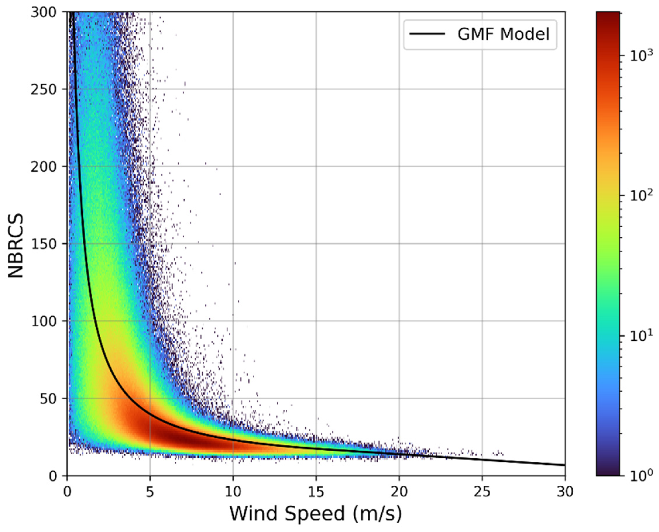
To fit the GMF model describing the relationship between wind speed and NBRCS, a constrained nonlinear least squares method is applied to the training and validation datasets. An iterative algorithm seeks the parameter set $\beta =[a_0,a_1,a_2,b_1,b_2]$. To prevent non-physical upward curvature in the high-wind-speed segment and ensure continuity and smooth transition at $u=15$, $b_2$ is constrained to be non-positive, and $b_0$ is not treated as a free fitting parameter but is calculated analytically using the continuity condition.

It is worth noting that the specific piecewise form of the GMF adopted in Equation (19) is not arbitrary, which typically employs a single analytical function over the full wind speed range; the piecewise strategy applied here offers greater flexibility in capturing the scattering saturation effect that occurs under high sea states. Specifically, the transition at 15 m/s decouples the retrieval into two regimes: a wind-dominated regime where NBRCS decreases monotonically with wind speed, and a roughness-saturated regime where the sensitivity of NBRCS to wind speed diminishes. By constraining $b_2\le 0$ during fitting, we enforce this physical saturation behavior, preventing the unphysical growth of NBRCS at extreme wind speeds that is sometimes observed in purely empirical fits.

The fitted scatter density plot is shown in Figure 4, with the curve representing the fitted GMF model. This model reflects the nonlinear dependency between wind speed and NBRCS. The obtained GMF model coefficients are [5.8744, 174.507, −23.531, 28.0192, −0.7077, −2.838 × 10⁻²].

4.2. Experimental Settings

This study builds and trains all deep learning models based on the PyTorch framework (version 2.0.1). Experiments are conducted on a machine equipped with an NVIDIA GeForce RTX 4090 GPU. To systematically evaluate the performance of each method, three common metrics are adopted: root mean square error (RMSE), bias and the coefficient of determination (R²), providing a multi-angle performance analysis. Models are trained for 100 epochs. If no decrease occurs for 10 consecutive epochs, an early stopping mechanism is triggered, improving training efficiency. The AdamW optimizer is used with an initial learning rate of 0.0005. We standardize all input data to enhance training stability and promote model convergence. The batch size is set to 512.

4.3. Ablation Study

To comprehensively evaluate the effectiveness of each core component in the proposed method and quantify its contribution, a systematic ablation study is conducted. These components include ancillary parameters, the physical loss function, the convolutional neural network, and the cross-attention mechanism. Exp. i serves as the baseline model, which employs only a Transformer encoder to extract features from the DDM, without any ancillary parameters, physical loss function, CNN, or cross-attention fusion. The results are shown in

Table 3. Ablation studies of specific components.

Exp.	Ancillary	LGMF	CNN	Cross-Attention	RMSE	Bias	R2
i					1.58	0.36	0.62
ii	√				1.46	0.30	0.68
iii		√			1.61	0.42	0.60
iv			√		1.52	0.31	0.62
v	√			√	1.32	0.13	0.77
vi	√	√			1.51	0.33	0.69
vii	√		√	√	1.31	0.15	0.77
viii	√	√	√		1.45	0.31	0.69
ix	√	√	√	√	1.35	0.22	0.75

.

(1) Impact of Ancillary Parameters: Based on the ablation results, we evaluate the performance gain after introducing ancillary data. Comparing the baseline experiment with the experiment group after introducing ancillary data (Exp. i vs. Exp. ii), it is found that introducing ancillary data significantly enhances the model’s overall retrieval capability. With only ancillary data introduced and no change to other modules, the RMSE decreases from 1.58 m/s to 1.46 m/s, and the R² increases from 0.62 to 0.68. The overall bias decreases from 0.36 m/s to 0.30 m/s, indicating that ancillary data provide the necessary physical constraints for the model, effectively correcting systematic bias arising from relying solely on DDMs. This suggests that DDM image features alone are insufficient to fully deconstruct the complex nonlinear relationship of sea surface wind fields, while the observational geometry and system parameters contained in ancillary data provide crucial prior information, complementing the limitations of unimodal data.

As shown in

Table 4. Ablation studies of specific components in different wind speed zones.

Exp.	Wind Speed < 5 m/s		5 m/s < Wind Speed < 10 m/s		10 m/s <Wind Speed < 15 m/s		Wind Speed > 15 m/s
	RMSE	Bias	RMSE	Bias	RMSE	Bias	RMSE	Bias
i	1.36	0.52	1.44	0.34	2.27	−1.47	5.14	−5.02
ii	1.24	0.64	1.31	0.09	2.01	−1.23	4.83	−4.54
iii	1.41	0.72	1.43	0.35	2.47	−1.36	4.74	−4.11
iv	1.28	0.49	1.36	0.10	2.42	−1.75	5.33	−4.99
v	1.16	0.40	1.19	0.02	1.92	−1.08	5.06	−4.42
vi	1.27	0.71	1.14	0.12	2.05	−1.06	4.53	−3.83
vii	1.13	0.40	1.15	0.07	2.14	−1.18	5.10	−4.77
viii	1.22	0.56	1.21	0.11	2.07	−0.81	4.62	−3.75
ix	1.29	0.67	1.15	0.18	2.02	−1.14	4.51	−3.90

, segmented error statistics further reveal the differential contribution of ancillary data across wind speed intervals. Comparing Exp. i and Exp. ii, in the 5–10 m/s interval, the RMSE significantly drops from 1.44 m/s to 1.31 m/s, and the bias sharply decreases from 0.34 m/s to 0.09 m/s. In the < 5 m/s interval, the RMSE decreases from 1.36 m/s to 1.24 m/s. These results indicate that in the low-to-medium wind speed range where sea surface roughness changes are more sensitive, the influence of geometric parameters on signal scattering characteristics is particularly significant. By fusing these scalar features, the model can more accurately decouple the joint effects of geometry and wind speed on NBRCS, enhancing stability in the low-to-medium wind speed range.

(2) Impact of the Physical Loss Function: Introducing ${\mathcal{L}}_{GMF}$ aims to regularize the purely data-driven neural network through the physical model (GMF). By comparing Exp. i vs. Exp. iii and Exp. ii vs. Exp. vi, the unique role of this physical constraint in addressing the high-wind-speed retrieval bottleneck and the performance trade-offs it brings can be observed.

The most significant change in experimental data is observed in the >15 m/s high-wind-speed interval. In GNSS-R retrieval, purely data-driven models often tend to underestimate extreme wind speeds. Comparing Exp. i vs. Exp. iii, the bias in the >15 m/s interval is reduced from 5.02 m/s to 4.11 m/s. This indicates that ${\mathcal{L}}_{GMF}$ successfully introduces physical scattering mechanisms into the loss function, maintaining a more reasonable response across the large dynamic range, thereby effectively suppressing severe negative bias at high wind speeds.

Comparing Exp. i vs. Exp. iii and Exp. ii vs. Exp. vi, it can be observed that after introducing ${\mathcal{L}}_{GMF}$, the global RMSE and R² show a slight performance regression or fluctuation. This phenomenon is typical in multi-objective optimization. The essence of ${\mathcal{L}}_{GMF}$ is a strong regularization term that forces predictions to conform to an empirical physical formula. However, the empirical GMF itself may have fitting errors, and the complexity of real sea states may deviate from the ideal GMF curve. When forcing the network to satisfy physical constraints for high wind speeds, some statistical goodness of fit in the low-to-medium-wind-speed segments is sacrificed. This can also be seen in the segmented table: in the < 5 m/s and 5–10 m/s intervals, the RMSE after introducing the GMF is typically slightly higher than in groups without it.

(3) Impact of the Convolutional Neural Network: Introducing the CNN module aims to replace simple linear projection to capture the local spatial structure with significant physical meaning in DDM images.

Compared to the baseline experiment, the CNN module demonstrates superior feature encoding capability over fully connected layers. Without using ancillary data or a GMF, replacing the feature extractor from a linear layer to a CNN reduces the RMSE from 1.58 m/s to 1.52 m/s and optimizes the bias from 0.36 m/s to 0.31 m/s. On a stronger baseline already including ancillary data and a GMF, introducing the CNN still brings performance improvement, with the bias remaining stable. DDM images are not unordered pixel sets; their energy distribution exhibits high spatial correlation along the delay and Doppler axes. CNN kernels can effectively extract local texture features and preserve key spatial topological information through pooling or stride operations, thereby more accurately characterizing sea surface roughness than simple linear mapping.

Segmented error statistics reveal the CNN’s unique advantage in the low-wind-speed segment (<5 m/s). In the <5 m/s interval, introducing the CNN reduces the RMSE from 1.36 m/s to 1.28 m/s. By comparing Exp. vi and Exp. viii, similarly in the <5 m/s interval, the CNN group’s RMSE is 1.22 m/s, superior to the non-CNN group’s 1.27 m/s. Under low wind speeds, the sea surface is relatively smooth, and the “horseshoe” region in DDM images is narrow with concentrated energy. Linear layers easily overlook these subtle morphological changes, while the CNN, through its local receptive field, can sensitively capture edge features in signal-concentrated regions, achieving finer low-wind-speed retrieval.

However, comparing Experiment v with Experiment vii, we can see that, when the model already incorporates cross-attention mechanisms and auxiliary parameters, the additional inductive bias introduced by the CNN can sometimes lead to overfitting due to the extremely imbalanced sample distribution, or conflict with the global modeling capabilities of the Transformer—particularly under high-wind-speed conditions where data are scarce. This explains why incorporating a CNN actually degrades performance at higher wind speeds, further highlighting the critical role of a GMF in mitigating the underestimation of high-wind-speed samples.

(4) Impact of the Cross-Attention Mechanism: The cross-attention mechanism is designed to replace traditional feature concatenation, enabling dynamic interaction between DDM image features and auxiliary scalar features.

The introduction of the cross-attention mechanism yields the most significant performance improvement among all ablation modules. From Exp. ii vs. Exp. v, it is found that with the same input data, merely changing the fusion method from concatenation to cross-attention reduces the RMSE from 1.46 m/s to 1.32 m/s, and increases the R² from 0.68 to 0.77. The global bias decreases from 0.30 m/s to 0.13 m/s. This result strongly proves that simple feature concatenation cannot fully exploit nonlinear inter-modal associations. The cross-attention mechanism allows image features to adaptively “retrieve” relevant geometric or system information from ancillary data based on their own needs, achieving deep alignment in feature space.

Segmented error statistics show that cross-attention demonstrates advantages across all wind speed intervals. The RMSE for Exp. v decreased to 1.16 m/s, significantly better than Exp. ii’s 1.24 m/s. The attention mechanism can more precisely utilize auxiliary parameters like the SNR to weight image features. In the >15 m/s interval, despite lacking a GMF constraint, Exp. v’s RMSE and bias are still slightly better than Exp. i’s baseline, and the final integrated model Exp. ix achieves an RMSE of 4.51 m/s in this interval.

Although Experiment vii achieved the best overall performance, its predicted values were significantly lower for samples with higher wind speeds; in contrast, Experiment ix, which ultimately integrated all modules, performed excellently across all wind speed ranges, with a root mean square error (RMSE) of 1.35 m/s, a bias of 0.22 m/s, and a coefficient of determination (R²) of 0.75.

4.4. Comparison with Other Deep Learning Methods

In this section, the proposed PA-HCTN is compared with several deep learning methods for GNSS-R wind speed retrieval, including the traditional retrieval algorithm Minimum Variance Estimator (MVE), MCNN, which uses CNN for wind speed estimation, and PA-CNN [41].

Table 5. Comparative study of different models.

Model	RMSE (m/s)	Bias (m/s)	R2 (-)
MVE	1.57	0.37	0.61
MCNN	1.44	0.25	0.67
PA-CNN	1.41	0.28	0.71
PA-HCTN	1.35	0.22	0.75

presents the quantitative estimation results for all comparative methods. From the perspective of global metrics, the PA-HCTN achieved a reduced RMSE of 1.35 m/s and an improved coefficient of $R^2$ of 0.75. Compared to the MVE, this represents an approximate 14% reduction in the RMSE. Furthermore, the performance gain over the peer physics-aware model, PA-CNN, validates the superiority of the proposed Hybrid CNN–Transformer architecture. This demonstrates that in the fusion of physical scalars and image features, the dynamic interaction mechanism based on cross-attention can more effectively uncover deep cross-modal correlations compared to traditional CNN feature concatenation strategies. Regarding the bias, the PA-HCTN, with an overall bias of only 0.22 m/s, outperforms both the MCNN and PA-CNN.

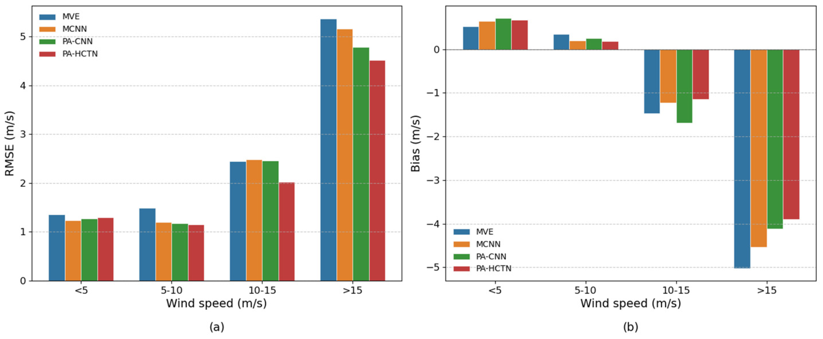
The segmented error statistics, presented in

Table 6. Comparative study of different models in different wind speed zones.

Model	Wind Speed < 5 m/s		5 m/s < Wind Speed < 10 m/s		10 m/s < Wind Speed 5 m/s		Wind Speed > 15 m/s
	RMSE	Bias	RMSE	Bias	RMSE	Bias	RMSE	Bias
MVE	1.36	0.52	1.49	0.34	2.44	−1.47	5.36	−5.02
MCNN	1.24	0.64	1.20	0.20	2.48	−1.23	5.15	−4.54
PA-CNN	1.27	0.71	1.17	0.25	2.46	−1.69	4.78	−4.11
PA-HCTN	1.29	0.67	1.15	0.18	2.02	−1.14	4.51	−3.90

, reveal the varying capabilities of different models in coping with complex sea states, with the PA-HCTN demonstrating optimal performance in the medium-to-high-wind-speed regimes. Specifically, in the 10–15 m/s interval—a transitional interval where retrieval difficulty increases steeply—existing models deteriorate to an RMSE exceeding 2.44 m/s. In contrast, the PA-HCTN successfully reduces this value to 2.02 m/s and significantly mitigates the bias to −1.14 m/s. For the range > 15 m/s, the PA-HCTN achieves an RMSE of 4.51 m/s and a bias of −3.90 m/s, significantly outperforming the MVE. This illustrates that by fusing physical constraints via cross-attention, the model can more accurately reconstruct nonlinear scattering relationships under high sea states, effectively mitigating severe underestimation. Figure 5 shows the histogram of the segmentation results.

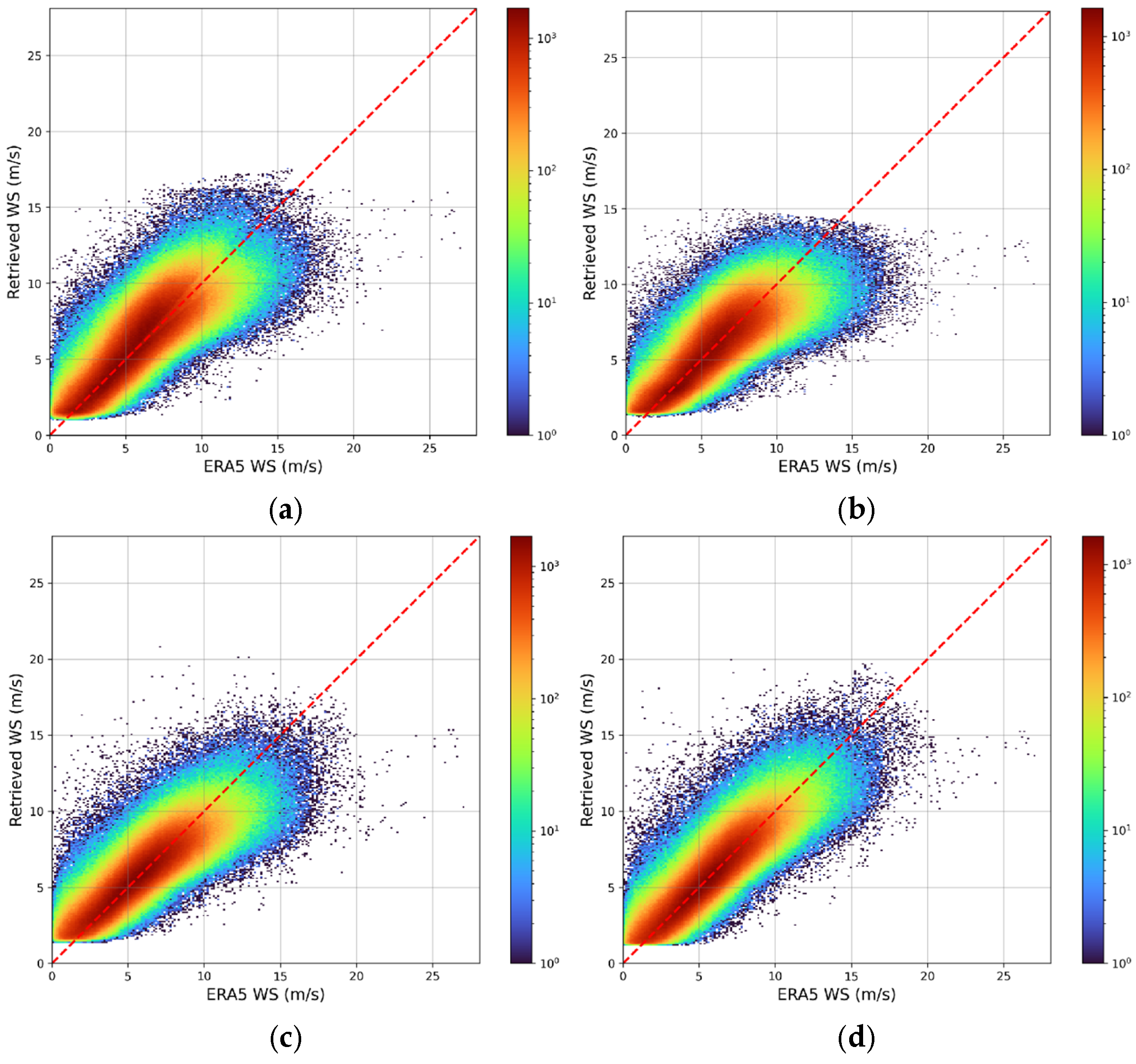
Figure 6 visually presents the scatter density plots comparing the retrieved wind speeds (y-axis) against the ERA5 reference wind speeds (x-axis) for the four comparative models across the entire test set. The color gradient, ranging from deep blue to dark red, represents the logarithmic density of the data points, with the red dashed line indicating the ideal $y=x$ diagonal.

The high-density core region of the PA-HCTN exhibits the most compact morphology and aligns most closely along the $y=x$ diagonal. In contrast, the core regions of the MVE and MCNN display a broader divergence, indicating larger prediction variance and a greater prevalence of estimates deviating from the ground truth. Furthermore, it is notable that both baselines exhibit significant underestimation for high-wind-speed samples. The PA-CNN demonstrates a marked convergence compared to the former two, and the incorporation of the GMF partially mitigates the underestimation issue; however, it still retains a degree of dispersion in the high-wind regime. By contrast, the scatter cloud of the PA-HCTN exhibits the optimal linear extension trend in the high-wind-speed segment. Although minor underestimation persists, its point cloud distribution adheres more closely to the diagonal. This further confirms the effectiveness of integrating the GMF and the cross-attention mechanism.

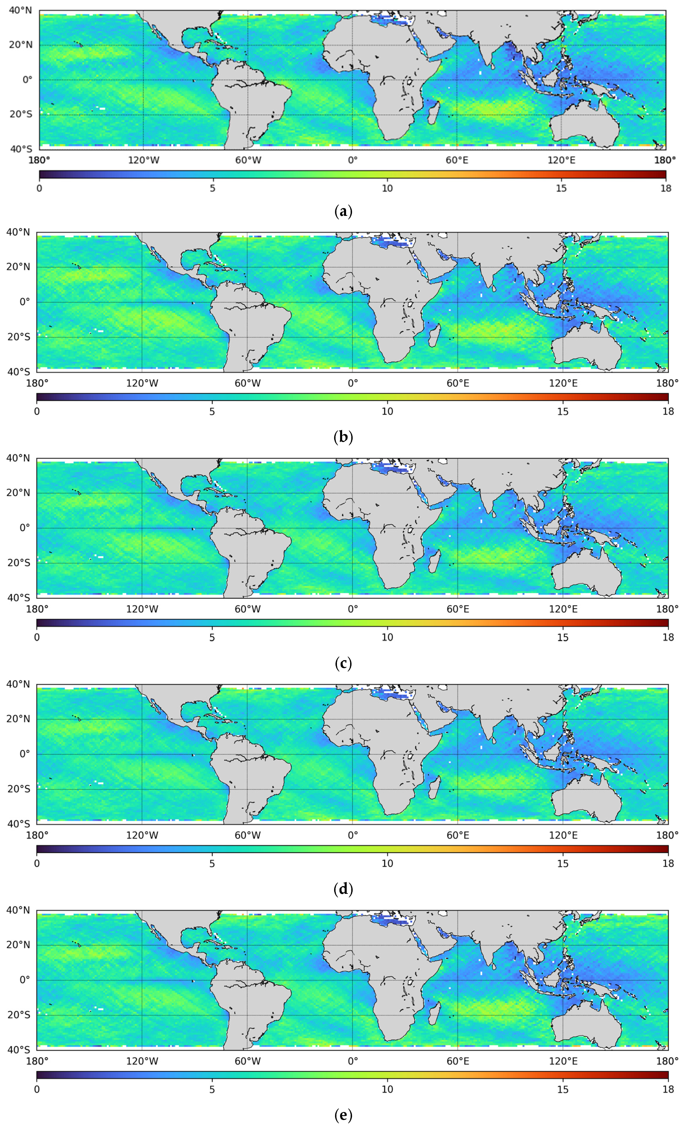
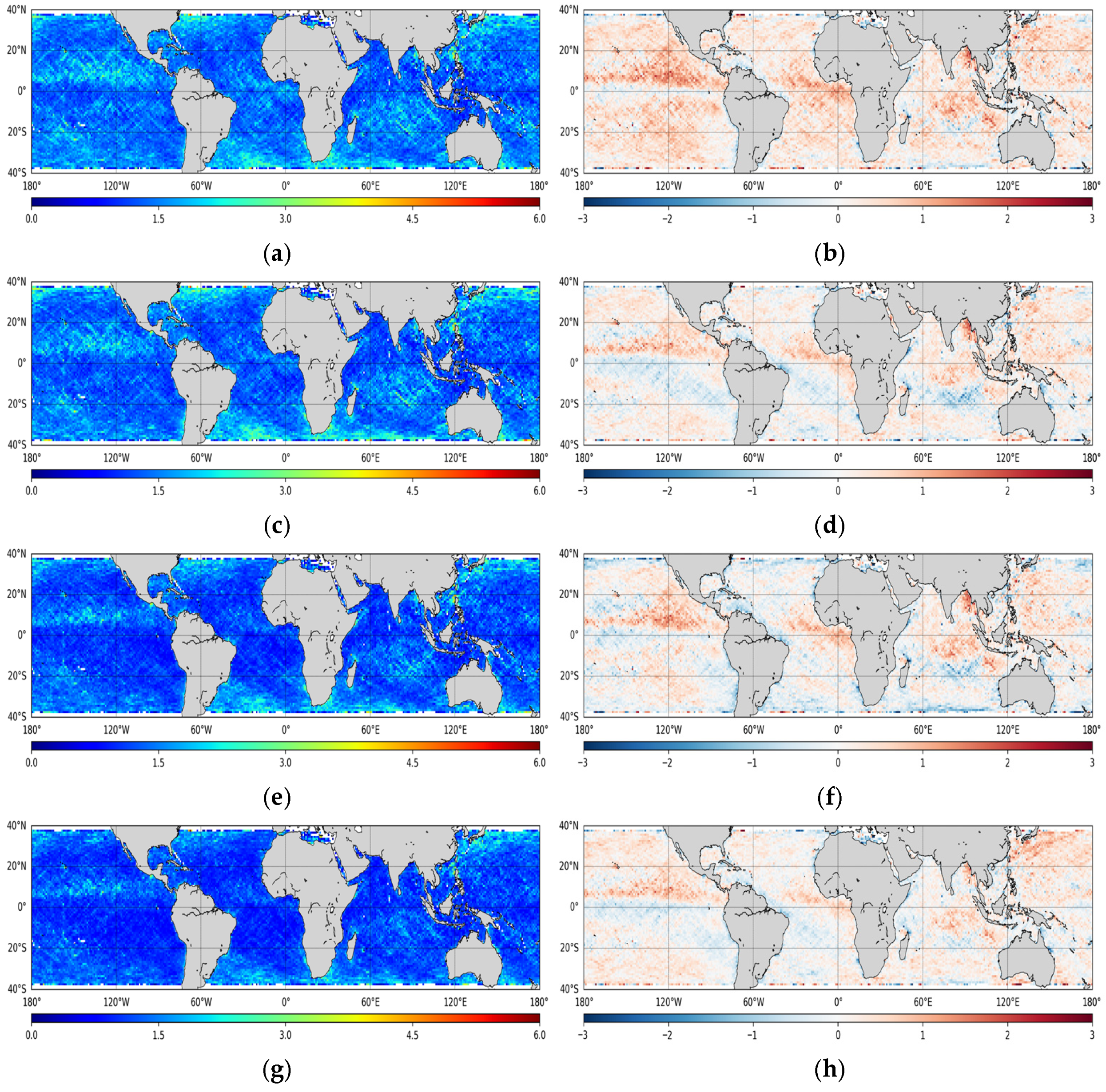
Figure 7 displays the global distribution of wind speeds averaged over a four-month test period at a 1° resolution, comparing ERA5 labels with retrievals from the four models. It can be observed that high wind speeds are predominantly located in open ocean regions. Quantitative comparison of these wind maps indicates that the global overall trends align well with the ground truth, with the PA-HCTN model’s estimates showing the closest agreement with ERA5. When examining the RMSD distribution maps in Figure 8, the proposed method also demonstrates superior performance; the generated map exhibits more deep blue regions, indicating RMSD values close to zero, whereas other methods show a higher RMSD. These qualitative results reflect the high consistency between the estimated wind speeds and the ERA5 reference data, validating the effectiveness of the proposed method in producing accurate and spatially consistent wind speed retrievals.

4.5. Validation with NDBC Buoy Measurements

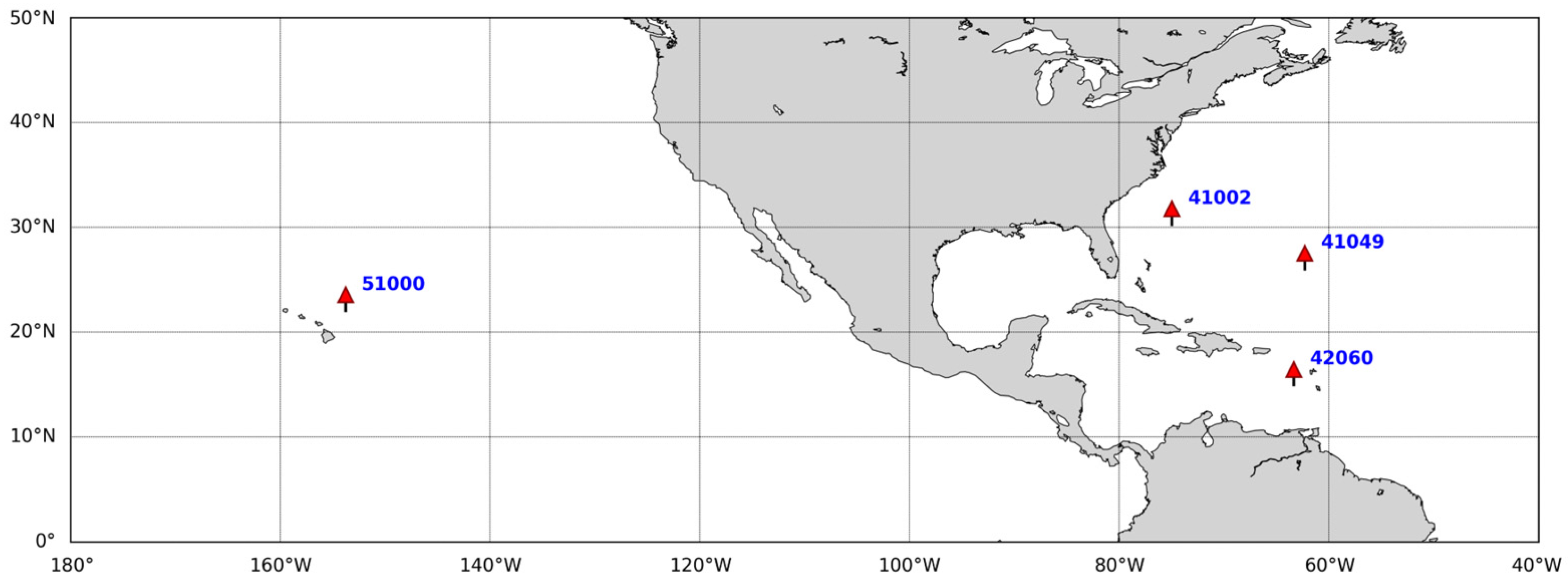
While ERA5 reanalysis provides a globally consistent reference, it is itself a model product with inherent uncertainties. To provide a more rigorous assessment of the PA-HCTN model’s performance in real-world conditions, we further validate it against independent in situ observations from NDBC buoys. NDBC buoy data provide in situ measurements from various locations, serving as a more accurate foundation for evaluating the performance of different models. In this study, four NDBC buoy stations were selected, as illustrated in Figure 9, The red arrows indicate the locations of the buoy stations. The dataset covers the time period from 1 September to 31 December 2024, which aligns with the time range of the test data.

Table 7. Comparison of different models against NDBC buoy measurements.

Buoy Station	Latitude (°N)	Longitude (°W)	MVE (m/s)	MCNN (m/s)	PA-CNN (m/s)	PA-HCTN (m/s)
41002	31.743	74.955	1.62	1.59	1.55	1.49
41049	27.505	62.271	1.57	1.53	1.49	1.45
42060	14.536	53.136	1.69	1.66	1.61	1.57
51000	23.534	153.752	1.70	1.61	1.56	1.54

presents a comparison between wind speeds estimated by four models and those measured by buoys, detailing the selected NDBC buoy stations and the root mean square errors for each model. Notably, the RMSE of the PA-HCTN model ranges from 1.45 to 1.51 m s⁻¹. Compared with the ERA5 validation results, an increase in the RMSE is expected, attributable to representative errors arising from comparing point-based buoy measurements with satellite-derived spatial coverage, as well as inherent uncertainties in the buoy measurements themselves. Across all four stations, the PA-HCTN consistently outperforms the other models. This consistent performance across diverse geographic locations robustly demonstrates the effectiveness and generalization capability of the proposed physically aware hybrid network.

5. Conclusions

In this study, we proposed the Physics-Aware Hybrid CNN–Transformer Network. By synergizing a CNN–Transformer hybrid encoder with a physics-guided cross-attention mechanism, our model effectively fuses delay–Doppler image features with auxiliary parameters. Furthermore, the integration of a GMF-constrained loss function explicitly enforces physical consistency, preventing the model from violating scattering laws and thus effectively combating underestimation in data-sparse high-wind regimes.

Utilizing CYGNSS Level 1 data, our experiments demonstrate that the model achieves a global RMSE of 1.35 m/s, representing a 14% improvement over standard Transformer baselines. Most critically, it significantly mitigates the persistent underestimation problem in high-wind-speed conditions (>15 m/s), reducing the bias to −3.90 m/s and exhibiting superior robustness compared to existing methods.

Despite these advancements, limitations remain. The current physical constraint relies on an empirical GMF, which may not fully capture complex sea state interactions. In addition, the computational complexity of this model poses challenges for real-time deployment. Future work will focus on two key directions: firstly, incorporating more rigorous theoretical electromagnetic scattering models to further enhance physical interpretability; and secondly, optimizing the model’s computational efficiency to enable lightweight deployment for real-time, on-board processing on future GNSS-R satellites.

References

1. Zheng, C.W.; Li, C.Y.; Pan, J.; Liu, M.Y.; Xia, L.L. An overview of global ocean wind energy resource evaluations. Renew. Sustain. Energy Rev. 2016, 53, 1240–1251. [Google Scholar] [CrossRef] [Scilit]
2. Han, Y.; Mi, L.; Shen, L.; Cai, C.; Liu, Y.; Li, K.; Xu, G. A short-term wind speed prediction method utilizing novel hybrid deep learning algorithms to correct numerical weather forecasting. Appl. Energy 2022, 312, 118777. [Google Scholar] [CrossRef] [Scilit]
3. Carswell, J.R.; Knapp, E.J.; Chang, P.S.; Black, P.; Marks, F. Limitations of scatterometry high wind speed retrieval. In Proceedings of the IEEE 2000 International Geoscience and Remote Sensing Symposium (IGARSS), Honolulu, HI, USA, 24–28 July 2000; Volume 3, pp. 1226–1228. [Google Scholar]
4. Shi, X.; Duan, D.; Ren, K. A More Accurate Field-to-Field Method towards the Wind Retrieval of HY-2B Scatterometer. Remote Sens. 2021, 13, 2419. [Google Scholar] [CrossRef] [Scilit]
5. Ding, F.; Zhao, C.; Chen, Z.; Deng, M.; Wang, T. Wind speed extraction from first-order sea echoes using a small-aperture multifrequency high-frequency radar. IEEE Trans. Geosci. Remote Sens. 2022, 60, 4206908. [Google Scholar] [CrossRef] [Scilit]
6. La, T.V.; Messager, C. Different Observations of Sea Surface Wind Pattern Under Deep Convection by Sentinel-1 SARs, Scatterometers, and Radiometers in Collocation. IEEE J. Sel. Top. Appl. Earth Obs. Remote Sens. 2022, 15, 3686–3696. [Google Scholar] [CrossRef] [Scilit]
7. Huang, W.; Liu, X.; Gill, E.W. Ocean Wind and Wave Measurements Using X-Band Marine Radar: A Comprehensive Review. Remote Sens. 2017, 9, 1261. [Google Scholar] [CrossRef] [Scilit]
8. Wyatt, L.R. Progress towards an HF Radar Wind Speed Measurement Method Using Machine Learning. Remote Sens. 2022, 14, 2098. [Google Scholar] [CrossRef] [Scilit]
9. Jing, C.; Li, W.; Wan, W.; Lu, F.; Niu, X.; Chen, X.; Rius, A.; Cardellach, E.; Ribó, S.; Liu, B.; et al. A review of the BuFeng-1 GNSS-R mission: Calibration and validation results of sea surface and land surface. Geo-Spat. Inf. Sci. 2024, 27, 638–652. [Google Scholar] [CrossRef] [Scilit]
10. Li, Z.; Guo, F.; Chen, F.; Zhang, Z.; Zhang, X. Wind speed retrieval using GNSS-R technique with geographic partitioning. Satell. Navig. 2023, 4, 4. [Google Scholar] [CrossRef] [Scilit]
11. Xing, J.; Yu, B.; Yang, D.; Li, J.; Shi, Z.; Zhang, G.; Wang, F. A real-time GNSS-R system for monitoring sea surface wind speed and significant wave height. Sensors 2022, 22, 3795. [Google Scholar] [CrossRef] [Scilit]
12. Bu, J.; Yu, K.; Ni, J.; Huang, W. Combining ERA5 data and CYGNSS observations for the joint retrieval of global significant wave height of ocean swell and wind wave: A deep convolutional neural network approach. J. Geod. 2023, 97, 81. [Google Scholar] [CrossRef] [Scilit]
13. Yan, Q.; Huang, W. Spaceborne GNSS-R sea ice detection using delay-Doppler maps: First results from the UK TechDemoSat-1 mission. IEEE J. Sel. Top. Appl. Earth Obs. Remote Sens. 2016, 9, 4795–4801. [Google Scholar] [CrossRef] [Scilit]
14. Rodriguez-Alvarez, N.; Holt, B.; Jaruwatanadilok, S.; Podest, E.; Cavanaugh, K.C. An Arctic sea ice multi-step classification based on GNSS-R data from the TDS-1 mission. Remote Sens. Environ. 2019, 230, 111202. [Google Scholar] [CrossRef] [Scilit]
15. Jin, Y.; Ji, M.; Zheng, N.; Zhang, Z.; Ding, P.; Zhao, Q. Soil moisture retrieval from TM-1 GNSS-R reflections with auxiliary geophysical variables: A multi-cluster and seasonal evaluation. Land 2025, 15, 36. [Google Scholar] [CrossRef] [Scilit]
16. Martín-Neira, M. A passive reflectometry and interferometry system (PARIS): Application to ocean altimetry. ESA J. 1993, 17, 331–355. [Google Scholar]
17. Rodriguez-Alvarez, N.; Munoz-Martin, J.F.; Morris, M. Latest advances in the global navigation satellite system—Reflectometry (GNSS-R) field. Remote Sens. 2023, 15, 2157. [Google Scholar] [CrossRef] [Scilit]
18. Zhang, L.; Qin, W.; Gao, F.; Kang, W.; Zhu, Y. Drone Height from Ground Determination Using GNSS-R Based on Dual-Frequency GPS/BDS Signals. Remote Sens. 2025, 17, 1722. [Google Scholar] [CrossRef] [Scilit]
19. Zhang, C.; Liu, X.; Ni, J.; Bu, J.; Zhan, Y.; Tao, D. SCAWaveNet: A Spatial-Channel Attention-based Network for Global Significant Wave Height Retrieval. arXiv 2025, arXiv:2507.00701. [Google Scholar] [CrossRef] [Scilit]
20. Foti, G.; Gommenginger, C.; Jales, P.; Unwin, M.; Shaw, A.; Robertson, C.; Roselló, J. Spaceborne GNSS reflectometry for ocean winds: First results from the UK TechDemoSat-1 mission. Geophys. Res. Lett. 2015, 42, 5435–5441. [Google Scholar] [CrossRef] [Scilit]
21. Carreno-Luengo, H.; Crespo, J.A.; Akbar, R.; Bringer, A.; Warnock, A.; Morris, M.; Ruf, C. The CYGNSS mission: On-going science team investigations. Remote Sens. 2021, 13, 1814. [Google Scholar] [CrossRef] [Scilit]
22. Rahmani, M.; Asgari, J.; Asgarimehr, M. Soil moisture retrieval using space-borne GNSS reflectometry: A comprehensive review. Int. J. Remote Sens. 2022, 43, 5173–5203. [Google Scholar] [CrossRef] [Scilit]
23. Jin, S.; Camps, A.; Jia, Y.; Wang, F.; Martin-Neira, M.; Huang, F.; Yan, Q.; Zhang, S.; Li, Z.; Edokossi, K.; et al. Remote sensing and its applications using GNSS reflected signals: Advances and prospects. Satell. Navig. 2024, 5, 19. [Google Scholar] [CrossRef] [Scilit]
24. Ruf, C.S.; Balasubramaniam, R. Development of the CYGNSS geophysical model function for wind speed. IEEE J. Sel. Top. Appl. Earth Obs. Remote Sens. 2019, 12, 66–77. [Google Scholar] [CrossRef] [Scilit]
25. Clarizia, M.P.; Ruf, C.S. Wind speed retrieval algorithm for the cyclone global navigation satellite system (CYGNSS) mission. IEEE Trans. Geosci. Remote Sens. 2016, 54, 4419–4432. [Google Scholar] [CrossRef] [Scilit]
26. Guo, W.; Du, H.; Cheong, J.W.; Southwell, B.J.; Dempster, A.G. GNSS-R wind speed retrieval of sea surface based on particle swarm optimization algorithm. IEEE Trans. Geosci. Remote Sens. 2021, 60, 4202414. [Google Scholar] [CrossRef] [Scilit]
27. Yan, Q.; Huang, W.; Moloney, C. Neural networks based sea ice detection and concentration retrieval from GNSS-R Delay-Doppler maps. IEEE J. Sel. Top. Appl. Earth Obs. Remote Sens. 2017, 10, 3789–3798. [Google Scholar] [CrossRef] [Scilit]
28. Yan, Q.; Huang, W. Detecting sea ice from TechDemoSat-1 data using support vector machines with feature selection. IEEE J. Sel. Top. Appl. Earth Obs. Remote Sens. 2019, 12, 1409–1416. [Google Scholar] [CrossRef] [Scilit]
29. Wang, C.; Yu, K.; Zhang, K.; Bu, J.; Qu, F. Significant wave height retrieval based on multivariable regression models developed with CYGNSS data. IEEE Trans. Geosci. Remote Sens. 2023, 61, 4200415. [Google Scholar] [CrossRef] [Scilit]
30. Wang, C.; Yu, K.; Qu, F.; Bu, J.; Han, S.; Zhang, K. Spaceborne GNSS-R wind speed retrieval using machine learning methods. Remote Sens. 2022, 14, 3507. [Google Scholar] [CrossRef] [Scilit]
31. Liu, X.; Bai, W.; Xia, J.; Huang, F.; Yin, C.; Sun, Y.; Du, Q.; Meng, X.; Liu, C.; Hu, P.; et al. FA-RDN: A hybrid neural network on GNSS-R sea surface wind speed retrieval. Remote Sens. 2021, 13, 4820. [Google Scholar] [CrossRef] [Scilit]
32. Xie, H.; Cheng, X.; He, S.; Li, Y.; Pang, J.; Li, S. MF-ANN: A novel artificial neural network-based method for ocean wind speed retrieval on spaceborne GNSS-R signal. IEEE Trans. Geosci. Remote Sens. 2023, 61, 5802617. [Google Scholar] [CrossRef] [Scilit]
33. Asgarimehr, M.; Arnold, C.; Weigel, T.; Ruf, C.; Wickert, J. GNSS reflectometry global ocean wind speed using deep learning: Development and assessment of CYGNSSnet. Remote Sens. Environ. 2022, 269, 112801. [Google Scholar] [CrossRef] [Scilit]
34. Arabi, S.; Asgarimehr, M.; Kada, M.; Wickert, J. Hybrid CNN-LSTM deep learning for track-wise GNSS-R ocean wind speed retrieval. Remote Sens. 2023, 15, 4169. [Google Scholar] [CrossRef] [Scilit]
35. Zhao, D.; Heidler, K.; Asgarimehr, M.; Arnold, C.; Xiao, T.; Wickert, J.; Zhu, X.X.; Mou, L. DDM-Former: Transformer networks for GNSS reflectometry global ocean wind speed estimation. Remote Sens. Environ. 2023, 294, 113629. [Google Scholar] [CrossRef] [Scilit]
36. Qiao, X.; Yan, Q.; Huang, W. Hybrid CNN-Transformer Network With a Weighted MSE Loss for Global Sea Surface Wind Speed Retrieval from GNSS-R Data. IEEE Trans. Geosci. Remote Sens. 2025, 63, 4207013. [Google Scholar] [CrossRef] [Scilit]
37. Du, H.; Li, W.; Cardellach, E.; Ribó, S.; Rius, A.; Nan, Y. Deep residual fully connected network for GNSS-R wind speed retrieval and its interpretation. Remote Sens. Environ. 2024, 313, 114375. [Google Scholar] [CrossRef] [Scilit]
38. Xu, Y.; Han, M.; Zheng, N.; Feng, Y.; Dai, Y. WsCBAM: A novel CBAM-based method for ocean wind speed retrieval from CYGNSS L1 by spaceborne GNSS-R technology. Meas. Sci. Technol. 2025, 36, 106140. [Google Scholar] [CrossRef] [Scilit]
39. CYGNSS. CYGNSS Level 1 Science Data Record Version; CYGNSS: Ann Arbor, CA, USA, 2021. [Google Scholar]
40. Hersbach, H.; Bell, B.; Berrisford, P.; Hirahara, S.; Horányi, A.; Muñoz-Sabater, J.; Nicolas, J.; Peubey, C.; Radu, R.; Schepers, D.; et al. The ERA5 global reanalysis. Q. J. R. Meteorol. Soc. 2020, 146, 1999–2049. [Google Scholar] [CrossRef] [Scilit]
41. Qiao, X.; Huang, W. Ocean Surface Wind Speed Estimation from GNSS-R Data Using Physics-Informed Attention-Aided Convolutional Neural Network. IEEE Trans. Geosci. Remote Sens. 2025, 63, 4210116. [Google Scholar] [CrossRef] [Scilit]
Figure 1. Overall structure of the PA-HCTN.
Remotesensing 18 01053 g001
Figure 2. Typical sea surface DDM image.
Remotesensing 18 01053 g002
Figure 3. Schematic diagram of Multi-Head Self-Attention mechanism.
Remotesensing 18 01053 g003
Figure 4. GMF fitting model.
Remotesensing 18 01053 g004
Figure 5. RMSE of different models across wind speed ranges: (a) RMSE, (b) bias.
Remotesensing 18 01053 g005
Figure 6. Density plots in log-scale for four methods against ERA5 wind speeds. Results of (a) MVE, (b) MCNN, (c) PA-CNN, (d) PA-HCTN.
Remotesensing 18 01053 g006
Figure 7. Geographical distribution of average wind speed: (a)ERA5, (b) MVE, (c) MCNN, (d) PA-CNN, (e) PA-HCTN.
Remotesensing 18 01053 g007
Figure 8. Average RMSE and bias spatial distributions. (a,b) MVE, (c,d) MCNN, (e,f) PA-CNN, (g,h) PA-HCTN.
Remotesensing 18 01053 g008
Figure 9. Location of NDBC buoy station.
Remotesensing 18 01053 g009