MSF-PhyDRNN: A Physics-Driven Multi-Source Fusion Recurrent Neural Network for Short-Term Thunderstorm Gale Nowcasting

Highlights

What are the main findings?

• The proposed MSF-PhyDRNN model effectively integrates radar and surface wind data using a novel multi-source fusion module and a lightweight PredRNN++ based recurrent unit.
• By introducing a dynamic weighted mean squared error loss function, the model significantly improves extreme wind prediction, achieving average increases of 14.3% in CSI, 27.2% in POD, and 19.7% in HSS compared to the advanced MFWPN model.

What are the implications of the main findings?

• This physics-driven framework successfully addresses the limitations of existing deep learning approaches, particularly mitigating performance decay at high wind speed thresholds.
• Accurate short-term nowcasting of highly destructive thunderstorm gales provides a critical and robust tool for mitigating wind-related disasters and protecting life and property.

Abstract

Accurate nowcasting of thunderstorm gales, a highly destructive form of severe convective weather, is critical for mitigating wind-related disasters and ensuring the safety of life and property. Existing deep learning approaches face challenges such as performance decay at high wind speed thresholds, limited capability in capturing extreme events, and difficulties in processing high-resolution data. To address these issues, this paper proposes a novel physics-driven multi-source fusion recurrent neural network named MSF-PhyDRNN. The model incorporates a multi-source fusion module that integrates radar composite reflectivity and surface wind field data through feature decoupling and hierarchical fusion. Additionally, we improved the recurrent unit in PhyDNet to enhance short-term wind capture and reduce redundancy, leveraging its cascaded memory and spatiotemporal propagation mechanisms. Experimental results indicate that, compared to the advanced MFWPN model, MSF-PhyDRNN achieves an average increase of 14.3% in the Critical Success Index (CSI), 27.2% in the Probability of Detection (POD), and 19.7% in the Heidke Skill Score (HSS) across the Jiangsu and South China datasets.

1. Introduction

Thunderstorm gale nowcasting refers to the utilization of historical meteorological observations to predict the future occurrence and evolution of severe convective weather. Essentially, it is a wind speed prediction task that fundamentally centers on the spatiotemporal forecasting of near-surface wind speeds. This process provides critical data support for severe convective weather warnings and plays a pivotal role in mitigating the impacts of sudden and destructive wind disasters. Accurate nowcasting significantly enhances the timeliness and reliability of early warnings, bearing profound implications for disaster prevention and mitigation, public safety, and the safeguarding of infrastructure and transportation. Consequently, in-depth research and the optimization of thunderstorm gale nowcasting methods are crucial for advancing modern meteorological disaster prevention systems and emergency management practices.

Current wind speed prediction methods are broadly categorized into physics-based modeling and data-driven approaches. Physics-based methods simulate atmospheric flow dynamics by solving complex systems of thermodynamic and hydrodynamic equations. Representative models include the Weather Research and Forecasting (WRF) model and various Integrated Forecasting Systems (IFS) [1,2]. These methods can yield high spatiotemporal resolution and physically interpretable wind field predictions when supported by high-quality input data. However, they face critical limitations in real-time operational nowcasting. Specifically, the complex data assimilation processes and iterative solving of partial differential equations demand continuous high-performance computing resources during the execution phase, often resulting in prolonged lag times. This inherent latency makes it difficult to provide the rapid, minute-level updates required for 0–2 h short-term severe convective forecasting, thereby limiting their operational flexibility and timeliness [3,4].

Data-driven methods mainly include statistical models and traditional machine learning algorithms. Classical statistical models such as ARIMA capture temporal wind speed variations [5,6,7], and improved versions combined with wavelet transforms or detrending operations have also been proposed [8,9]. However, their linear assumptions make them incapable of modeling strong nonlinear and non-stationary characteristics of wind fields, especially for long forecasting horizons and rapidly changing intensities. Traditional machine learning methods including SVM, artificial neural networks, and support vector regression have been widely adopted in wind speed prediction [10,11,12,13]. Despite reasonable performance on small datasets, these shallow models lack sufficient feature extraction ability for large-scale regional spatiotemporal data and rely on inefficient manual parameter tuning, making it difficult to satisfy real-time and high-precision forecasting requirements [14,15].

Deep learning, with its superior nonlinear feature modeling and automated representation learning capabilities, has garnered significant attention in wind speed forecasting [16]. Compared to traditional machine learning methods, deep learning models leverage deeper network architectures and hierarchical feature extraction to more accurately capture and fit the complex nonlinear spatiotemporal relationships in wind fields. Long Short-Term Memory (LSTM) networks [17], a cornerstone of time series forecasting, utilize unique memory and forget gate mechanisms to effectively capture long- and short-term temporal dependencies in sequential data. Building on this, Li et al. proposed a hybrid framework combining gated recurrent units with variational mode decomposition for interval prediction of short-term wind speeds [18]. Farah et al. developed a forecasting framework integrating data decomposition techniques with bidirectional LSTM to achieve precise short-term wind speed estimation [19]. Similarly, Wei et al. employed autoencoders and singular value decomposition to extract critical features from wind speed and related meteorological variables, followed by GRU-based modeling for single-point wind speed time series prediction [20]. These approaches, collectively termed single-point forecasting methods, primarily focus on time series modeling for individual observation sites. However, the wind, as a fluid medium, exhibits significant spatial correlations. Analyzing single-site data in isolation or simplistically modeling spatial correlations among limited sites, while neglecting regional spatiotemporal interactions, inevitably limits the model’s ability to represent complex wind field dynamics, thus constraining prediction accuracy.

Moving beyond the constraints of spatially isolated modeling, extensive research on spatiotemporal prediction has employed models like ConvLSTM, which integrates convolutional and recurrent networks to capture wind field dynamics. Yang et al. developed a deep attention convolutional recurrent model incorporating K-means clustering and enhanced memory mechanisms, leveraging attention layers, CNNs, and recurrent neural networks (RNNs) to deeply mine and represent spatiotemporal wind field features, significantly enhancing prediction performance [21]. Similarly, ref. [22], by combining UNet’s robust feature extraction and reconstruction capabilities with ConvLSTM’s spatiotemporal modeling, achieved accurate hourly solar radiation forecasts. However, LSTM-based models face challenges with gradient propagation in multi-layer architectures, leading to insufficient information aggregation and suboptimal accuracy in multi-step forecasting scenarios. The STDGN employs a self-attention separation strategy to effectively integrate spatial, temporal, and multivariate information, optimized with an uncertainty loss function for precise multi-variable meteorological forecasting [23]. Lin et al. proposed a model combining attention mechanisms and convolutional operations to enhance spatiotemporal feature extraction for high-accuracy offshore wind speed forecasting [24]. In wind speed prediction, model errors are primarily systematic, stemming from inadequate representation of deterministic physical processes, and uncertainty errors, arising from wind’s inherent randomness and uncontrollable factors [25]. Zhang et al. developed a deep learning model based on a convolution-self-attention architecture, integrating wind speed, temperature, terrain, and topography data through a spatiotemporal fusion module and composite loss function optimization, achieving high-precision short-term low-altitude wind field forecasts [26]. Although incorporating multivariate data, such as temperature and pressure, reduces prediction uncertainty, current multi-task forecasting methods have limitations. Notably, scalar wind speed forecasting offers distinct advantages over vector wind field analysis in disaster prevention. Unlike wind power generation, which requires precise vector UV wind field data for turbine angle adjustments, disaster mitigation prioritizes wind speed magnitude as a direct indicator of threats to structures, facilities, and human safety, providing clear risk quantification for emergency decision-making. Moreover, scalar wind speed forecasting avoids the computational complexity of resolving coupled wind direction and speed components, reducing model complexity and data processing costs, enabling rapid response in complex convective weather scenarios. Therefore, scalar wind speed forecasting presents a practical and efficient approach well-suited to the demands of real-time risk assessment and disaster prevention.

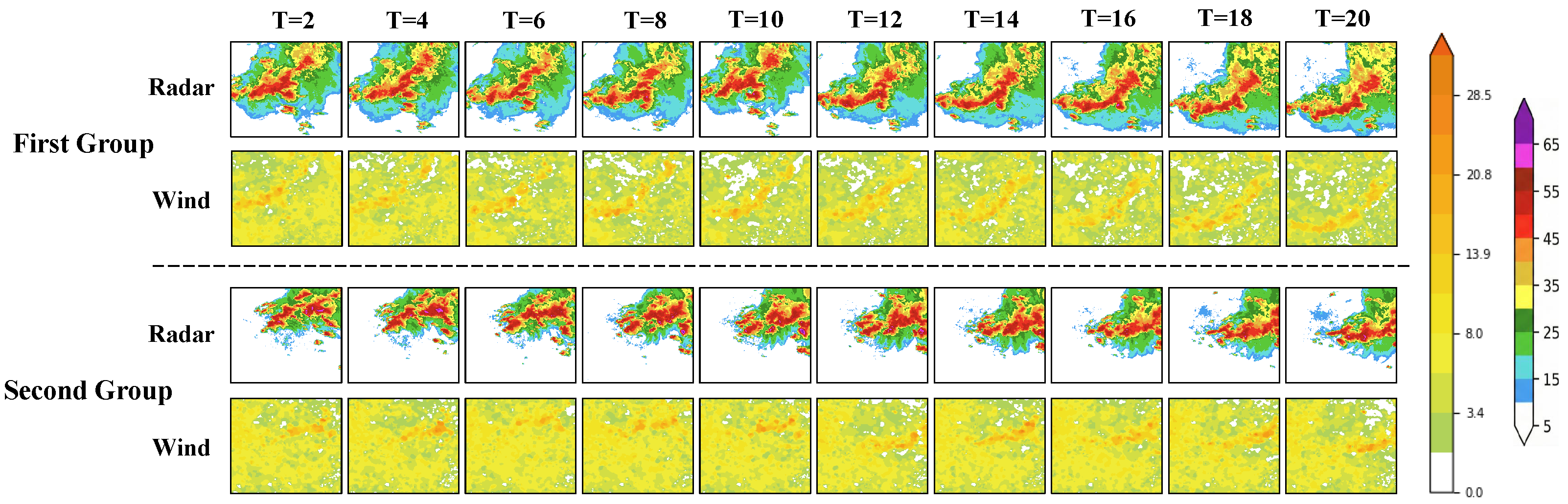
However, an efficient forecasting target must be supported by comprehensive and high-quality input data. Single data sources are inherently insufficient for the precise analysis and prediction of complex wind generation mechanisms. Integrating high-resolution radar composite reflectivity, which captures the vertical structure, horizontal extent, and movement of convective systems, with surface wind field observations reflecting near-surface wind speed, direction, and pulsation, enables highly complementary insights. As convective precipitation systems are primarily driven by higher-altitude steering flows rather than near-surface winds, the movement of radar reflectivity aloft serves as a crucial physical proxy representing the large-scale motion of these weather systems. This higher-altitude motion, in turn, dynamically guides the trajectories of large-scale variations in the near-surface wind field. Specifically, comparative analyses of historical weather events reveal that high-echo regions in S-band radar composite reflectivity exhibit a high degree of spatiotemporal coincidence and consistent movement trajectories with areas of high surface wind speed, as shown in Figure 1.

Although weather radars generally lack data in clear-air regions, thunderstorm gales are strongly coupled with intense precipitation cores. Thus, tracking these high-echo regions provides sufficient kinematic context for forecasting extreme winds. Furthermore, Doppler (radial) velocity is currently excluded due to physical and operational constraints. Physically, radial velocity primarily reflects mid-to-high altitude winds, whereas gale disasters are defined by near-surface winds (e.g., 10-m height), making automatic station observations an indispensable ground truth. Operationally, raw Doppler velocity suffers from severe aliasing (folding) in extreme winds. The massive computational overhead required for real-time de-aliasing poses a significant challenge for 0–2 h nowcasting. Therefore, fusing quality-controlled composite reflectivity with surface data ensures optimal model stability and computational efficiency while effectively addressing observational gaps. Ultimately, this targeted approach captures the physical lifecycle linking mesoscale systems to thunderstorm gales, improving overall forecast accuracy.

The main contributions of this work are summarized as follows:

To address these observational and methodological limitations, we propose MSF-PhyDRNN, a novel framework for fine-scale scalar wind speed forecasting. This method addresses the need for deterministic modeling of wind speed using a CNN-RNN-based spatiotemporal feature evolution module, incorporating a multi-source fusion module and a spatial feature encoder–decoder. To enable feature decoupling and integration of radar composite reflectivity and surface wind field data, we designed a multi-source fusion module employing a spatial attention mechanism and a cascaded cross-source feature refinement strategy. This preserves the integrity of features from both data sources while uncovering their spatiotemporal correlations through the attention mechanism. Additionally, to significantly reduce model parameters, we implemented a lightweight recurrent unit based on PredRNN++ [27] using a parameter-sharing strategy. By sharing convolutional kernels and gating parameters across layers and time steps, this approach mitigates overfitting risks and improves the consistency of feature learning. We then replaced the original ConvLSTM cell in PhyDNet [28] with this lightweight spatiotemporal unit, leveraging its superior spatiotemporal feature capture and long-term modeling capabilities to enhance the representation of nonlinear abrupt changes in convective systems. Finally, we designed a dynamic weighted mean squared error loss function that couples maximum wind speed physical boundaries with disaster assessment thresholds, assigning higher weights to convective winds approaching or exceeding these thresholds to enhance model accuracy for high-impact wind speeds.

• We propose a multi-source data fusion module that employs a spatial attention mechanism and a cascaded feature refinement approach to decouple and integrate radar composite reflectivity and surface wind field data. This module preserves the distinct characteristics of each data source while effectively capturing their spatiotemporal relationships.
• To enhance the PhyDNet architecture, we initially design a lightweight recurrent unit based on PredRNN++, utilizing a parameter-sharing strategy. We then replace the original ConvLSTM unit within PhyDNet with this lightweight cell. This modification leverages PredRNN++’s advanced spatiotemporal modeling to significantly reduce parameters without compromising generalization performance.
• We design a dynamic weighted mean squared error loss function that couples maximum wind speed physical constraints with disaster impact thresholds, assigning higher weights to thunderstorm gale samples to improve the model’s prediction accuracy for extreme wind events.
• Comprehensive experiments conducted on the Jiangsu and South China datasets validate the effectiveness and superiority of our method for thunderstorm gale nowcasting over state-of-the-art prediction approaches.

2. Data

The experiment was conducted on the South China 2021–2023 dataset and the 2022 Jiangsu Meteorological AI Algorithm Challenge dataset.

The South China 2021–2023 dataset comprises radar composite reflectivity data and surface wind speed observations from 2021 to 2023 in the South China region. The radar composite reflectivity data have a temporal resolution of 6 min and a spatial resolution of 0.01° (approximately 1 km), while the surface wind speed data have a temporal resolution of 5 min and a matching spatial resolution of 0.01°. The radar data were interpolated to align with the spatiotemporal resolution of the surface wind speed data. The data cover a region spanning 109.45°E to 117.20°E and 20.09°N to 25.31°N. This region, characterized by a subtropical monsoon climate, is a hotspot for thunderstorm gales. Influenced by land-sea thermal contrasts, it experiences frequent convergence of cold and warm air masses during summer, often compounded by typhoons and disturbances of the subtropical high, making it an ideal case study for wind speed forecasting. The dataset includes 13,294 wind events, each consisting of 24 consecutive frames (2 h), with an original spatial resolution of 600 × 800 pixels per frame. Due to computational constraints, the data were downsampled to 120 × 140 pixels using bilinear interpolation. From the total events, 11,136 samples were allocated to the training set and 2158 to the validation set, with pixel values normalized to the [0, 1] range.

The 2022 Jiangsu Meteorological Artificial Intelligence Algorithm Challenge dataset comprises radar composite reflectivity and automatic weather station data from Jiangsu, China, spanning April to September of 2019–2021. It includes quality-controlled, mosaicked S-band radar reflectivity factor data at a 3-km altitude and 6-min mean wind observations. The data cover a region from 116.18°E to 121.57°E and 30.45°N to 35.20°N. Located in the lower-middle Yangtze River Plain and near coastal and riverine areas, this region is influenced by disturbances from the subtropical high, low-pressure vortices, and northeast cold vortices. These conditions lead to frequent and complex thunderstorm gales, making the region an ideal area for wind speed forecasting studies related to wind disasters. The dataset has a spatial resolution of 0.01° (approximately 1 km) and a temporal resolution of 6 min, covering a grid of 480 × 560 pixels. Radar reflectivity ranges from 0 to 70 dBZ, while mean wind speed data, ranging from 0 to 30 m/s, are generated by interpolating automatic weather station observations onto a uniform grid using Inverse Distance Weighting (IDW) [29]. Although this interpolation introduces some errors and may not fully represent actual observations, it effectively utilizes sparse data to capture the spatial distribution of meteorological variables. Due to computational constraints and the large size of the original images, bilinear interpolation was applied to downsample the data to a 120 × 140 pixel resolution, with all values normalized to the [0, 1] range. A sliding window mechanism with a 40-time-step length was used, where the first 20 frames serve as model input and the subsequent 20 frames as prediction targets, forming input–output sample pairs. From the dataset, 26,328 valid sequence samples were obtained, split in a 9:1 ratio, with 23,695 samples for training and 2633 for validation.

3. Methods

3.1. Problem Definition

This study focuses on predicting thunderstorm gales in large-scale, fine-resolution grid-based wind fields, a task inherently defined as a four-dimensional modeling problem involving spatial (longitude, latitude), temporal, and variable dimensions. Specifically, the wind field is discretized into grid cells based on geographic coordinates, with each cell serving as an observation node for scalar wind speed, collectively forming a spatiotemporal dynamic system for prediction. Let $x_i\in {\mathbb{R}}^{C\times H\times W}$ denote the spatial distribution of the multidimensional variables at a specific time step i. A historical sequence of observation data over a period T can be expressed as ${\chi }^{T,t}=\{x_i\mid i\in [t-T+1,t]\}$, where t denotes the current time step, T denotes the historical time length, C denotes the number of variable channels, H denotes the latitudinal height, and W denotes the longitudinal width. In this study, the Jiangsu and South China datasets include radar composite reflectivity and mean scalar wind speed data; therefore, C is set to 2. Based on the historical sequence ${\chi }^{T,t}$, the wind speed sequence at the subsequent $T^{\prime }$ time steps, denoted as ${\mathrm{Y}}^{t,T^{\prime }}=\{x_i\mid i\in [t+1,t+T^{\prime }]\}$, can be obtained as:

$${\mathrm{Y}}^{t,T^{\prime }}={\mathcal{F}}_{\theta }\left({\chi }^{T,t}\right)$$

(1)

where ${\mathcal{F}}_{\theta }$ denotes the proposed MSF-PhyDRNN model parameterized by $\theta$.

3.2. MSF-PhyDRNN Overall Architecture

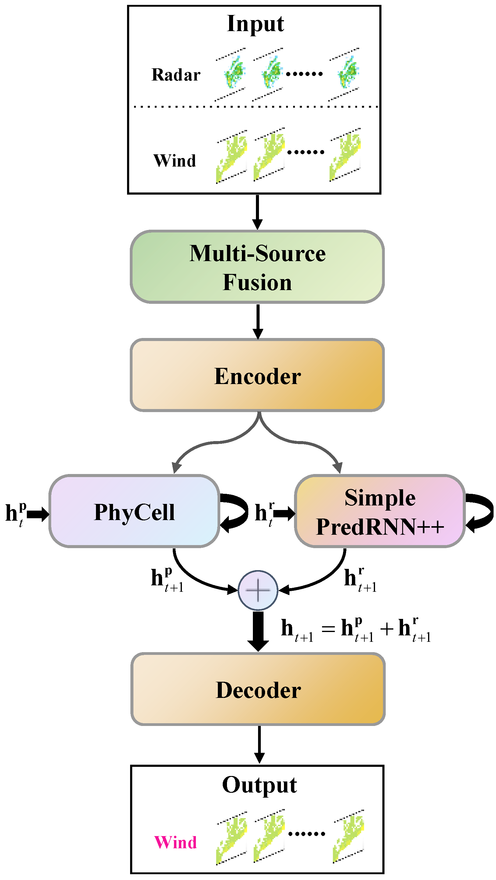
The model structure of MSF-PhyDRNN is shown in Figure 2. This model takes 20 consecutive frames (2 h) of radar composite reflectivity and surface wind field data as input and predicts the subsequent 20 frames (2 h) of scalar wind fields. The key components of the architecture include the Multi-Source Fusion module, the encoder, a dual-branch recurrent core consisting of PhyCell and Simple PredRNN++, and the decoder.

Specifically, the input sequences of radar composite reflectivity and surface wind field data are first integrated by the Multi-Source Fusion module and mapped into a high-dimensional hidden state space by the Encoder. The architecture then employs a disentangled spatiotemporal modeling strategy, routing these encoded features into two parallel recurrent branches. The PhyCell branch explicitly models the deterministic physical dynamics of the convective systems, updating the physical hidden state from $h_t^p$ to $h_{t+1}^p$. Operating in parallel, the Simple PredRNN++ branch captures the complex, nonlinear spatiotemporal residual features that physical equations cannot fully resolve, updating the residual hidden state from $h_t^r$ to $h_{t+1}^r$. The outputs from these two complementary branches are then aggregated via element-wise addition, formulated precisely as $h_{t+1}=h_{t+1}^p+h_{t+1}^r$, to form a comprehensive spatiotemporal representation for the current time step. Finally, the Decoder progressively maps this aggregated hidden state back to the original spatial resolution to generate the final output sequence of future scalar wind fields.

3.3. Multi-Source Fusion Module

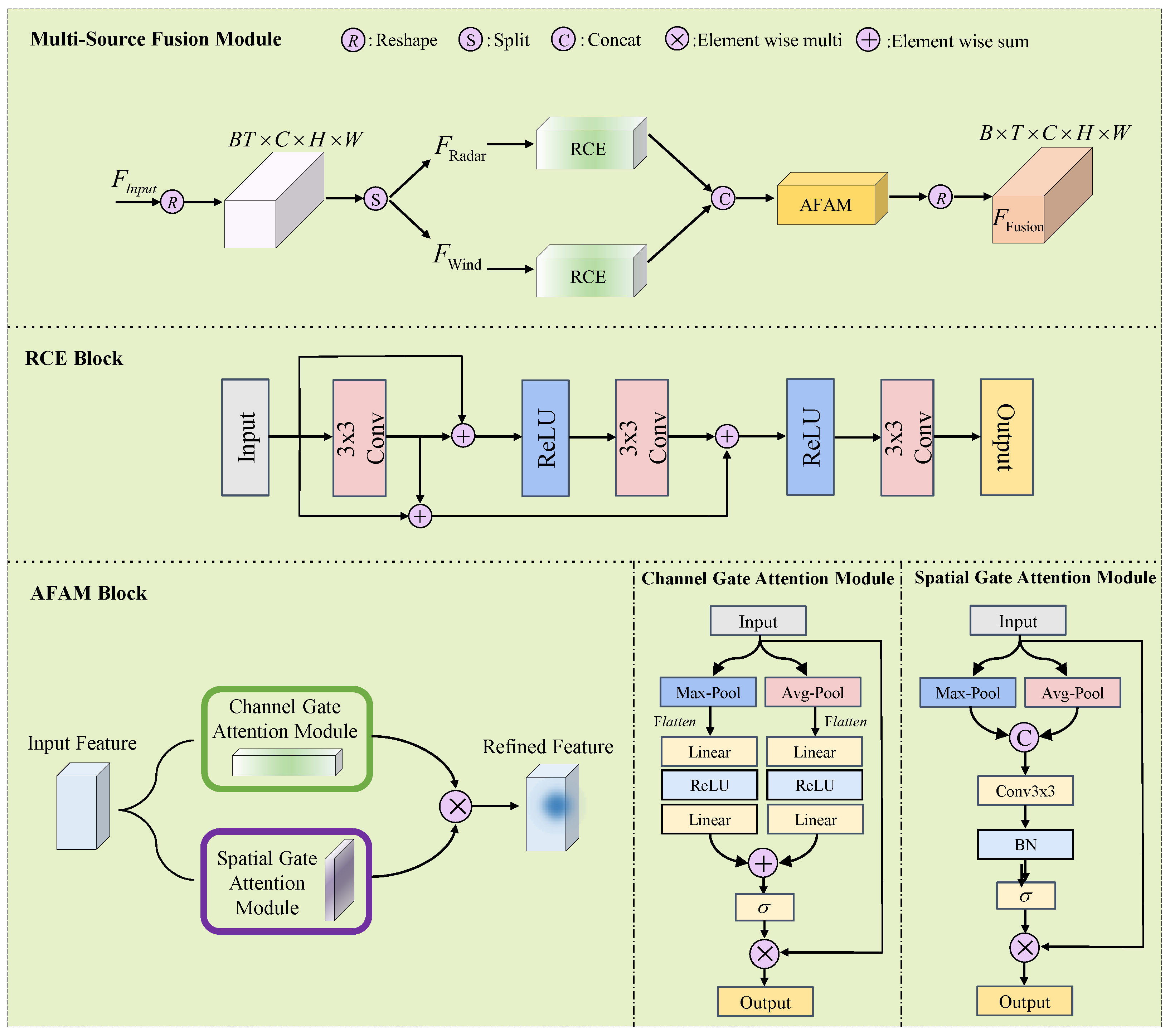
To effectively utilize radar composite reflectivity data for correcting wind field characteristics, we propose a multi-source data fusion module. Residual connections [30], which mitigate gradient vanishing in deep networks by combining raw inputs with convolved features, have proven effective in preserving feature integrity. Inspired by this, we introduce a Residual Convolution Enhancement (RCE) unit into the fusion module, employing a three-stage convolution with residual fusion to enhance the feature representation of both radar composite reflectivity and wind field data. Additionally, CBAM [31], known for enhancing key features through channel and spatial attention, inspires our Adaptive Fusion Attention Module (AFAM). AFAM integrates Channel Gated Attention (CGA) and Spatial Gated Attention (SGA) to precisely refine wind field evolution features using radar composite reflectivity data. Specifically, CGA aggregates channel statistics via global average and max pooling, generating channel weights through a multilayer perceptron to scale feature maps and emphasize channels strongly correlated with wind field evolution. SGA produces dual-channel feature maps by fusing mean and max values across channels, applying convolution and batch normalization to generate spatial weights that focus on key regions associated with high-wind cores. The output of AFAM acts on the original feature map by applying element-wise multiplication with the channel weights generated by CGA and the spatial weights generated by SGA, thereby achieving adaptive enhancement of wind field evolution features. This mechanism effectively suppresses irrelevant noise interference and significantly strengthens the feature signals of regions with strong wind cores and high wind shear.

As shown in Figure 3, the multi-source data fusion module consists of a residual convolutional enhancement unit and an adaptive fusion attention module. Specifically, the input tensor $F_{\mathrm{Input}}\in {\mathbb{R}}^{B\times T\times 2\times H\times W}$ is split along the channel dimension into $F_{\mathrm{Radar}}$ and $F_{\mathrm{Wind}}$, where $F_{\mathrm{Radar}},F_{\mathrm{Wind}}\in {\mathbb{R}}^{B\times T\times 1\times H\times W}$. These separated features are then fed into the corresponding RCE units for feature enhancement, which can be expressed as follows:

$$F_{\mathrm{Radar}},F_{\mathrm{Wind}}=\mathrm{Split}\left[R\left(F_{\mathrm{Input}}\right)\right]$$

(2)

$$F_{\mathrm{Radar}}^{\mathrm{E}}=\mathrm{RCE}\left(F_{\mathrm{Radar}}\right)$$

(3)

$$F_{\mathrm{Wind}}^{\mathrm{E}}=\mathrm{RCE}\left(F_{\mathrm{Wind}}\right)$$

(4)

where R denotes the dimension transformation from $B\times T\times C\times H\times W$ to $BT\times C\times H\times W$, and $\mathrm{Split}$ represents the segmentation computation. Taking $F_{Wind}\in {\mathbb{R}}^{BT\times 1\times H\times W}$ as an example, the calculation process of the RCE unit can be summarized as follows:

$$F_{Wind}^1=W_{3\times 3}^1\left(F_{Wind}\right)$$

(5)

$$F_{Wind}^2=W_{3\times 3}^2(ReLU(F_{Wind}^1+F_{Wind}))$$

(6)

$$F_{Wind}^{\mathrm{E}}=W_{3\times 3}^3(ReLU(F_{Wind}^1+F_{Wind}^2+F_{Wind}))$$

(7)

where $W_{3\times 3}$ denotes a $3\times 3$ convolution, and ReLU denotes the ReLU activation function. After that, $F_{Radar}^{\mathrm{E}}\in R^{BT\times 16\times H\times W}$ and $F_{Wind}^{\mathrm{E}}\in R^{BT\times 16\times H\times W}$ are concatenated along the channel dimension to form a multi-channel feature map. This concatenated feature map is then fed into the AFAM. The overall process can be summarized as follows:

$$F_{RW}=Cat[F_{Radar}^{\mathrm{E}};F_{Wind}^E]\in R^{BT\times 32\times H\times W}$$

(8)

$${\widehat{F}}_{\mathrm{Fusion}}=\mathrm{AFAM}\left(F_{RW}\right)\in R^{BT\times 32\times H\times W}$$

(9)

where $\mathrm{Cat}$ denotes feature splicing, and $\mathrm{AFAM}$ denotes an adaptive fusion attention module, which is designed to explore intrinsic relationships between radar reflectivity information and surface wind field information. The calculation process of this module can be summarized as follows:

$$\begin{array}{cc}\hfill SGA\left(F_{RW}\right)& =F_{RW}\odot \sigma \left(BN\right(W_{3\times 3}\left(Cat\right[\hfill \\ \hfill & \mathrm{AvgPool}\left(F_{RW}\right);MaxPool\left(F_{RW}\right)\left]\right)\left)\right)\hfill \end{array}$$

(10)

$$\begin{array}{cc}\hfill CGA\left(F_{RW}\right)=F_{RW}& \odot \sigma (MLP\left(\mathrm{AvgPool}\left(F_{RW}\right)\right)\hfill \\ \hfill & +MLP\left(MaxPool\left(F_{RW}\right)\right))\hfill \end{array}$$

(11)

$${\widehat{F}}_{\mathrm{Fusion}}=\mathrm{CGA}\left(F_{\mathrm{RW}}\right)\odot \mathrm{SGA}\left(F_{\mathrm{RW}}\right)$$

(12)

where $\mathrm{SGA}$ denotes the spatial gated attention, $\sigma$ denotes the sigmoid activation function, BN denotes the normalization layer, $\mathrm{Cat}$ denotes feature splicing, $\mathrm{AvgPool}$ and $\mathrm{MaxPool}$ denote average pooling and maximum pooling, $\mathrm{CGA}$ denotes the channel gated attention, MLP denotes a multilayer perceptron composed of two fully connected layers and ReLU activation functions, and ⊙ denotes element-wise multiplication. Finally, the dimension of ${\widehat{F}}_{\mathrm{Fusion}}\in R^{BT\times 32\times H\times W}$ is reshaped to obtain $F_{Fusion}\in R^{B\times T\times 32\times H\times W}$.

3.4. Simple PredRNN++ Recurrent Unit

The thunderstorm gale nowcasting task requires a spatiotemporal unit capable of stable long-term modeling, accurate capture of nonlinear abrupt changes, and seamless integration with the physics-constrained PhyDNet framework. Mainstream units struggle to meet these demands simultaneously. The classic ConvLSTM [15] relies on a single hidden state memory, making it highly susceptible to gradient vanishing in multi-layer, long-sequence scenarios, which leads to rapid accuracy degradation in 1–2 h forecasts. Furthermore, while MIM [32] introduces a high-order memory module, its underlying assumption of sequence stationarity limits its ability to capture the strongly nonlinear and abrupt dynamics of extreme thunderstorm gale events. In contrast, PredRNN++ effectively addresses these limitations. It employs a causal LSTM structure for decoupled spatial and temporal memory and introduces the Gradient Highway Unit (GHU). The GHU builds a direct gradient connection across time steps, fundamentally alleviating gradient vanishing and allowing for the stable transmission of key convective features over long sequences. Finally, its latent state representations can be seamlessly aggregated and jointly optimized with the physical hidden states of the PhyDNet branch without significant adaptation costs. Therefore, PredRNN++ serves as the ideal baseline for our lightweight recurrent unit design.

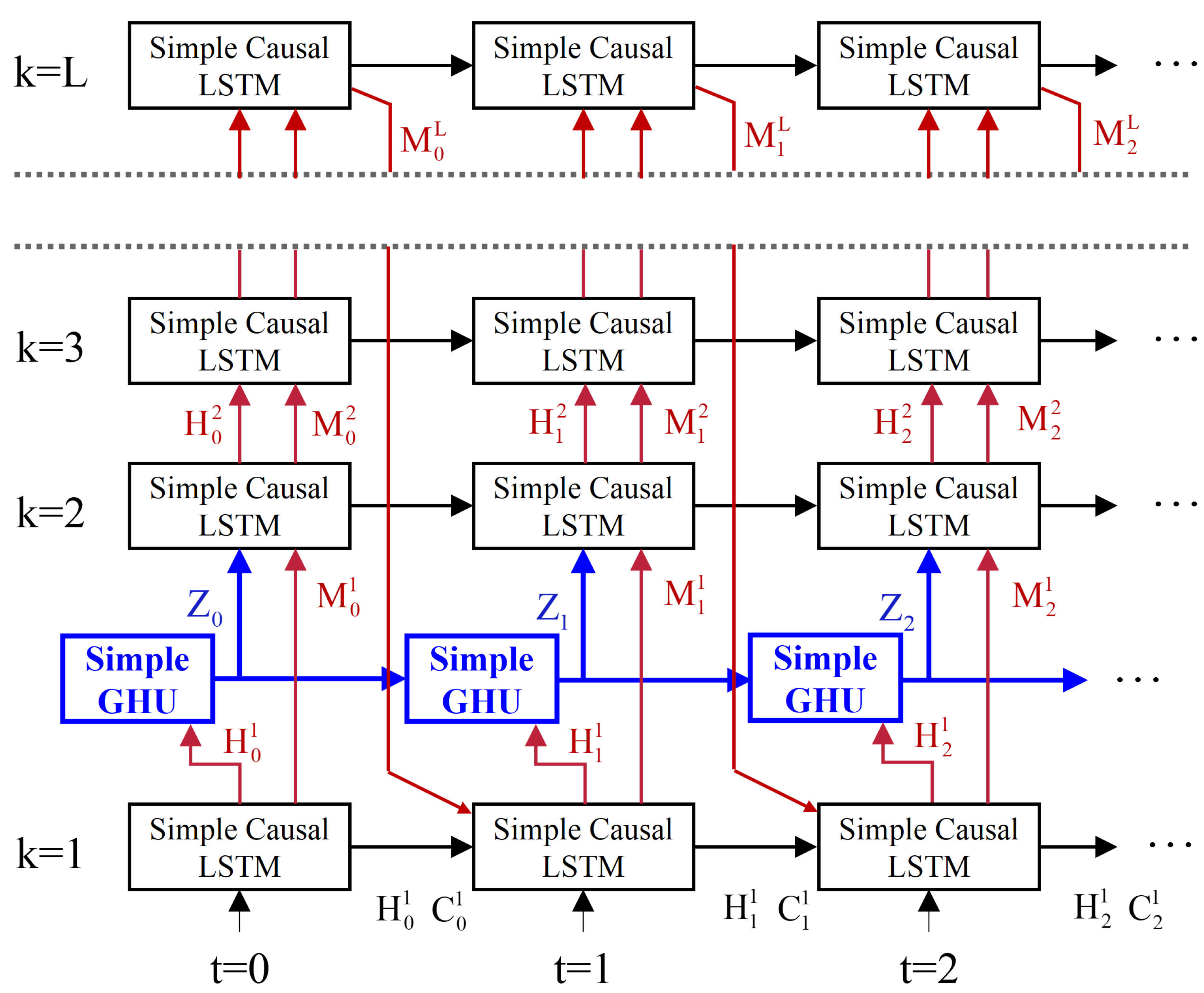
Building upon these theoretical advantages, we further tailored the PredRNN++ architecture specifically for high-resolution wind field temporal modeling by introducing optimizations centered on parameter sharing. The resulting lightweight recurrent unit retains the enhanced memory cell structure and spatiotemporal gating mechanisms of PredRNN++. By implementing a parameter-sharing strategy across time steps and model branches, the recurrent unit significantly reduces computational complexity and mitigates overfitting risks, all while preserving its robust capacity to capture long-term spatiotemporal dependencies. The detailed architecture is illustrated in Figure 4. Specifically, we stack three SimpleCausalLSTM layers and integrate a SimpleGHU (Gradient Highway Unit) between the first and second layers. This design effectively alleviates the difficulty of long-term gradient propagation inherent in stacked LSTMs, prevents the temporal memory from discarding critical historical wind field information, and enhances the overall stability of the recurrent architecture under complex disturbances or periodic variations.

As depicted in the structural design, SimpleCausalLSTM denotes a lightweight, improved version of CausalLSTM, designed to enhance computational efficiency without compromising temporal modeling capability. It consolidates multi-path convolutional operations by concatenating the input, the hidden state, and the memory unit before applying a single convolution to generate the gating signals, thereby significantly reducing computational branches. Furthermore, the gating mechanism is simplified by replacing multi-path convolutional additions with a direct splitting of the unified convolutional output. This effectively lowers parameter sensitivity and mitigates overfitting. Additionally, while retaining the core functionality of the gradient highway, SimpleGHU also features the advantages of a smaller parameter scale and higher computational efficiency. Ultimately, SimpleGHU and SimpleCausalLSTM achieve seamless collaboration, which are respectively used to capture long-term temporal dependencies and short-term dynamic changes in wind fields.

4. Experiments and Analysis

4.1. Implementation Details

In this study, all experiments were implemented using the PyTorch (version 2.1.2) deep learning framework and conducted on an NVIDIA RTX 4090 GPU (24 GB). To ensure scientific reproducibility, the specific model configurations and training hyperparameters are explicitly provided. Following the multi-source fusion module, the spatial encoder consists of a general encoder with 3 convolutional layers (with strides of 2, 1, and 2) and a specific encoder with 2 convolutional layers. This structure extracts deep hierarchical features, downsampling the spatial resolution by a factor of 4 while mapping the channel dimension to 64. The disentangled recurrent core operates through two parallel branches: the PhyCell branch consists of 1 layer with a hidden dimension of 64 and a $7\times 7$ convolutional kernel, while the Simple PredRNN++ branch is stacked with 3 layers, uniformly utilizing a hidden dimension of 64 and $5\times 5$ convolutional kernels for its spatiotemporal gates. The decoder symmetrically mirrors the encoder using transposed convolutions to progressively upsample the latent representations, culminating in a $1\times 1$ convolution that maps the final 32-channel features back to a single-channel scalar wind speed prediction at the original $120\times 140$ resolution. During the training phase, all models were trained for 80 epochs with a batch size of 8. The network weights were optimized using the Adam optimizer with an initial learning rate of $1\times {10}^{-3}$. To more accurately focus on the prediction error within high-wind regions, the model utilizes a Weighted Mean Squared Error (WMSE) loss function, which is an improved variant of the standard Mean Squared Error (MSE). This loss function incorporates a dynamic weighting mechanism specifically designed for high-wind characteristics. The weighting is based on the maximum wind speed value, applying an exponentially scaled weight to the true wind speed. This process generates a weight matrix that varies with wind speed, with its magnitude constrained within a threshold suitable for severe wind assessment. This design assigns higher weights to high-wind areas and lower weights to low-wind regions, thereby intensifying the model’s focus on learning high-wind features during training and ultimately enhancing prediction accuracy for high-wind events. The formula for the loss function is defined as follows:

$$W_{t,h,w}={10}^{\left({\displaystyle \frac{Y_{t,h,w}-10{log}_{10}\left(k\right)}{\alpha }}\right)}$$

(13)

$$L_{\mathrm{WMSE}}={\displaystyle \frac{1}{T\times H\times W}}\sum _{t=1}^T\sum _{h=1}^H\sum _{w=1}^W{W}_{t,h,w}·{(Y_{t,h,w}-{\tilde{Y}}_{t,h,w})}^2$$

(14)

where $Y_{t,h,w}$ denotes the actual wind speed value of the target sequence at pixel coordinates $(h,w)$ at timestamp t, ${\tilde{Y}}_{t,h,w}$ is the corresponding predicted wind speed value, and $W_{t,h,w}$ represents the dynamically calculated weight matrix for that specific pixel. Furthermore, k is the weight baseline coefficient used to establish the initial baseline for weight changes, and $\alpha$ is a constant scaling factor that controls the rate of the weight variation. In our experiments, k and $\alpha$ are empirically set to $16.0$ and $8.05$, respectively, which are optimized through extensive tuning in operational scenarios to appropriately penalize extreme wind errors. T is the total length of the predicted sequence, while H and W represent the height and width of the wind speed prediction field, respectively.

4.2. Evaluation Metrics

To comprehensively evaluate the performance of our model in the wind speed prediction task, we employed three standard meteorological evaluation metrics: the Critical Success Index (CSI) [33], Probability of Detection (POD) [34], and Heidke Skill Score (HSS) [35]. These metrics objectively quantify the predictive capacity and accuracy of the model. For performance evaluation, we applied a threshold $\tau$ to convert the predicted and ground-truth fields into binary matrices. Specifically, wind speed values above $\tau$ were set to 1, and 0 otherwise. Based on these binary matrices, a confusion matrix was further constructed to analyze the model’s wind speed prediction performance. In binary classification tasks, the confusion matrix, a standard tool for performance assessment, tabulates the correspondence between predicted and actual labels. As shown in

Table 1. Confusion Matrix for Binary Classification.

	Prediction: 1	Prediction: 0
Truth: 1	TP (true positive)	FN (false negative)
Truth: 0	FP (false positive)	TN (true negative)

, it includes true positives (prediction = 1, truth = 1, denoted as TP), false positives (prediction = 1, truth = 0, denoted as FP), true negatives (prediction = 0, truth = 0, denoted as TN), and false negatives (prediction = 0, truth = 1, denoted as FN). These statistics enable the calculation of CSI, POD, and HSS. In this study, experiments were conducted using three intensity thresholds: 1.6 m/s, 5.5 m/s, and 10.8 m/s.

The CSI, also known as the threat score (TS), is an essential measure of the accuracy of predicted wind events. In practical forecasting, it effectively penalizes both misses and false alarms, making it crucial for evaluating extreme wind speed warnings. The CSI value is calculated as follows:

$$\mathrm{CSI}={\displaystyle \frac{\mathrm{TP}}{\mathrm{TP}+\mathrm{FN}+\mathrm{FP}}}$$

(15)

The POD reflects the proportion of correct events predicted by the model to all actual correct events. In operational early warning systems, a higher POD indicates a stronger sensitivity to detecting hazardous winds, ensuring fewer actual thunderstorm gale events are missed. It is calculated as follows:

$$\mathrm{POD}={\displaystyle \frac{\mathrm{TP}}{\mathrm{TP}+\mathrm{FN}}}$$

(16)

HSS measures the predictive efficacy of the model by comparing the difference between the actual and stochastic prediction. It provides a robust assessment of forecasting skill, especially when the frequency of background non-events is overwhelmingly high. The formula for calculating the HSS is as follows:

$$\mathrm{HSS}={\displaystyle \frac{2\times (\mathrm{TP}\times \mathrm{TN}-\mathrm{FN}\times \mathrm{FP})}{(\mathrm{TP}+\mathrm{FN})\times (\mathrm{FN}+\mathrm{TN})+(\mathrm{TP}+\mathrm{FP})\times (\mathrm{FP}+\mathrm{TN})}}$$

(17)

The values of CSI and POD range from 0 to 1, and the HSS value varies between −1 and 1. The CSI, POD, and HSS can intuitively reflect the model’s performance for real-world applications, with higher values indicating better predictive performance.

4.3. Comparative Experiments

To thoroughly validate the advanced capabilities and effectiveness of the proposed MSF-PhyDRNN model, we compared it against several state-of-the-art benchmarks. The selected models include ConvLSTM [15], PredRNN++ [27], PhyDNet [28], MIM [32], SimVP [36], Earthfarsser [37], Diffcast [38], and MFWPN [26]. Among them, ConvLSTM, PredRNN++, and MIM represent classical spatiotemporal prediction algorithms, while PhyDNet, SimVP, Earthfarsser, Diffcast, and MFWPN are recognized as state-of-the-art nowcasting algorithms that have been widely applied to standard spatiotemporal tasks such as meteorological forecasting. The hyperparameters for all comparative models were configured based on their respective open-source implementations and were further fine-tuned according to the specific characteristics of our experimental task to ensure optimal performance. To guarantee a fair comparison, all models were trained on identical datasets and subjected to the same training protocols, including the use of a unified optimizer, learning rate, and number of training epochs.

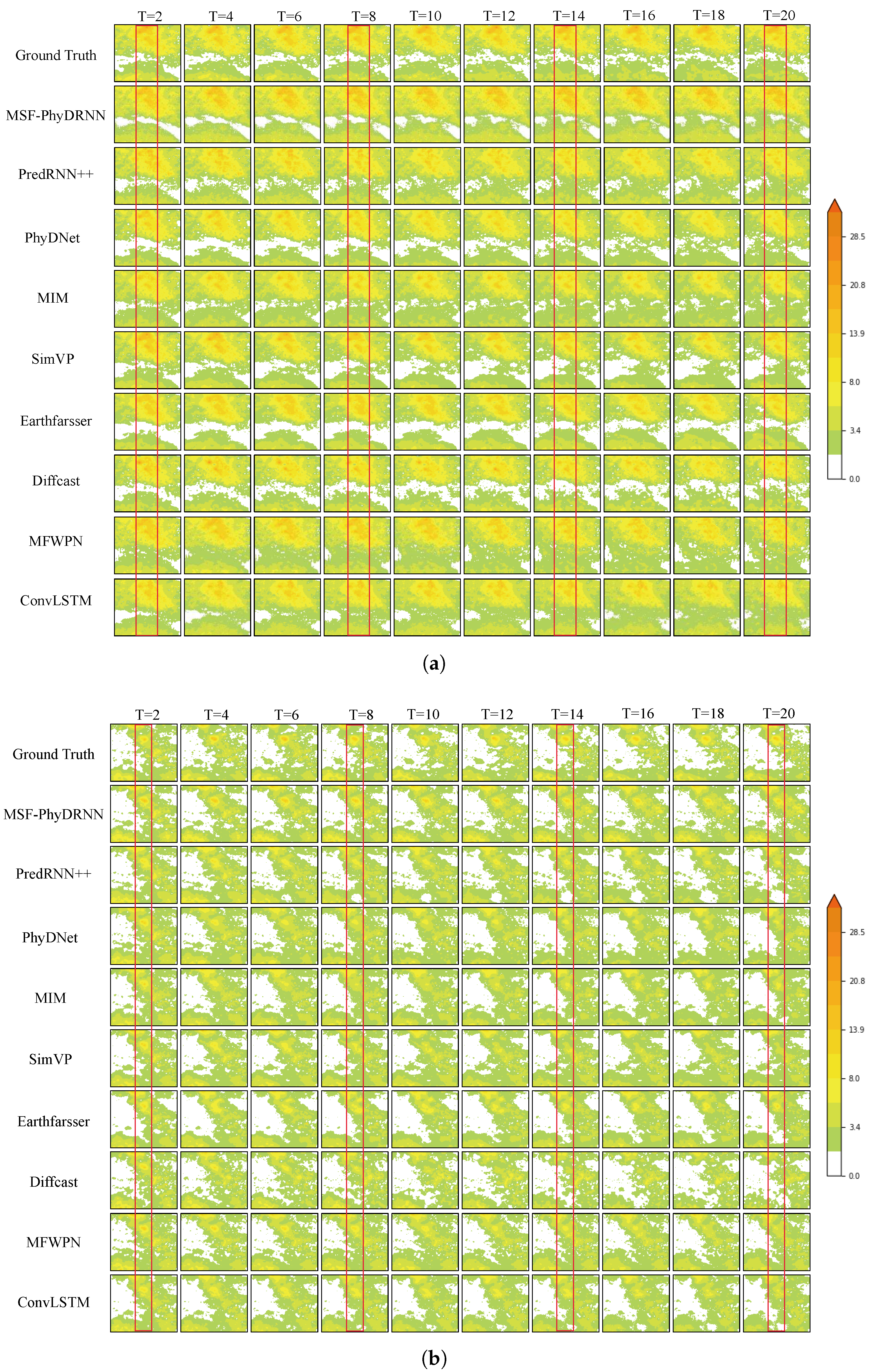
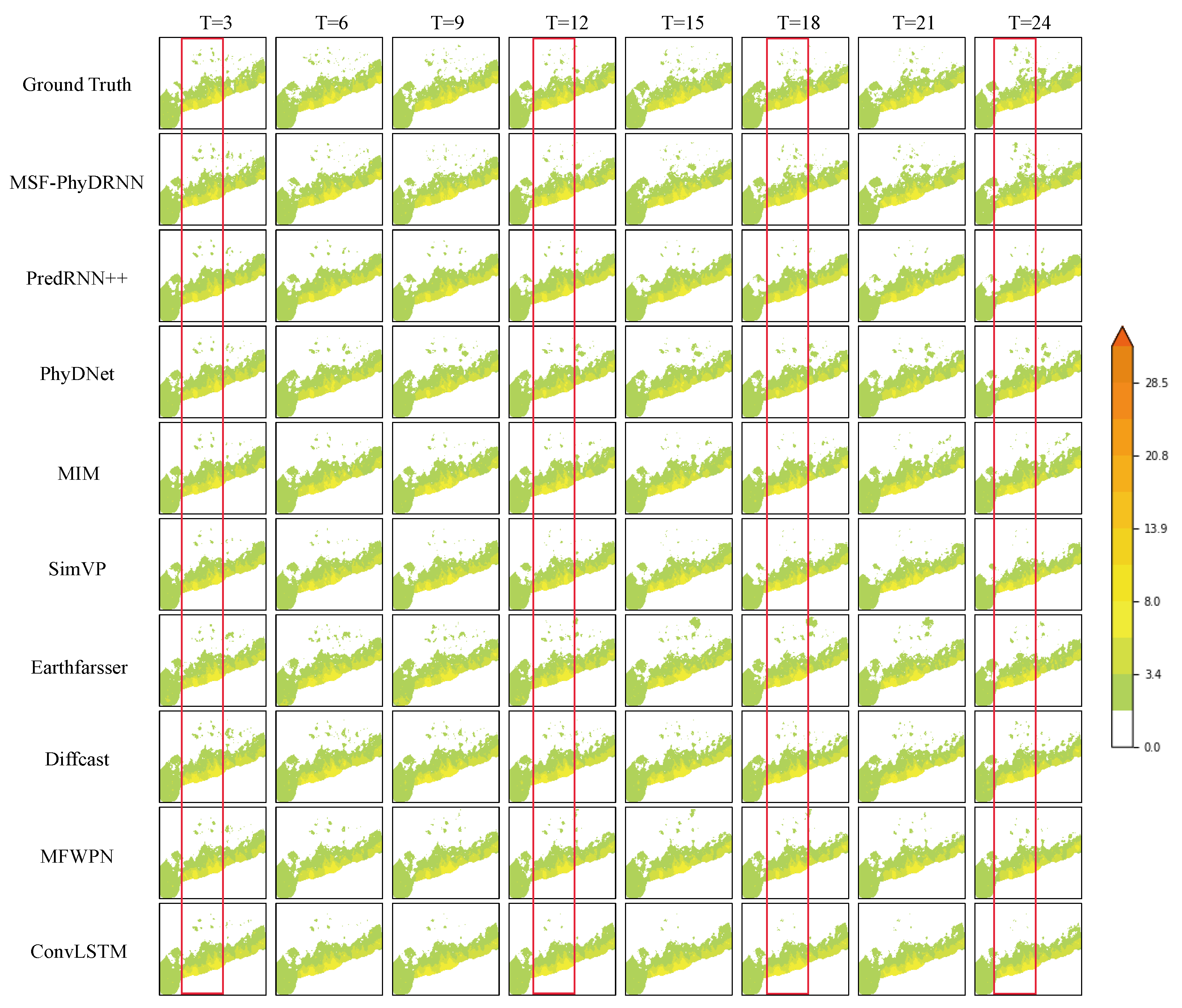
Figure 5a,b and Figure 6 illustrate the predictive performance of the proposed model across three distinct thunderstorm gale systems: multi-cell clusters, supercells, and boundary-layer convergence lines.

As depicted in Figure 5a, capturing a severe thunderstorm gale in Jiangsu Province, the observed wind field exhibits a concentrated spatial distribution moving from southwest to northeast. Qualitatively, all baseline models struggle to maintain the intensity of high-threshold wind regions, displaying varying degrees of underestimation compared to ground truth. Diffcast performs the poorest; its diffusion architecture lacks the adaptability needed for the abrupt spatiotemporal dynamics of severe convection. While ConvLSTM, PhyDNet, and MIM capture basic structural features, they degrade significantly in long-term forecasts due to constraints in modeling long-range spatiotemporal dependencies. SimVP and Earthfarsser predict motion trends relatively well, but their intensity predictions deteriorate markedly after the 12th time step ($t=12$). Benefiting from its multi-source fusion, MFWPN effectively captures morphological evolution, yet visual inspection still reveals a systematic underestimation of wind intensity. In contrast, the proposed MSF-PhyDRNN architecture demonstrates superior predictive accuracy and visual fidelity across these evaluated scenarios.As shown in Figure 5b, observations reveal a weakening trend in an individual convective cell. Models including ConvLSTM, PredRNN++, PhyDNet, MIM, SimVP, Earthfarsser, and Diffcast all failed to predict the development of this isolated convective cell. While MFWPN captured the development of the cell, it significantly underestimated its intensity, particularly from the 8th time step (t = 8) onward, with predictive quality deteriorating rapidly throughout the forecast horizon. In comparison, MSF-PhyDRNN accurately predicted both the position and intensity of the isolated convective cell, and its forecast of the cell’s movement trend showed high consistency with ground-truth observations throughout the time series.

For the case shown in Figure 6, while all models effectively capture the overall movement and morphology of the thunderstorm gales, most struggle with long-term intensity maintenance. Specifically, ConvLSTM, PredRNN++, PhyDNet, MIM, and SimVP exhibit premature attenuation of high-wind regions. For instance, the high-wind scope in ConvLSTM shrinks rapidly, while PhyDNet and MIM show severe underestimation starting from the 12th time step ($T=12$). Even PredRNN++ suffers from accelerated intensity decay despite its gradient highway mechanism. Conversely, MFWPN, Earthfarsser, and Diffcast maintain high-wind scopes well initially but generate false alarms in intensity during later stages. In contrast, the proposed MSF-PhyDRNN accurately tracks movement trends and stably maintains high-wind intensities throughout the entire prediction horizon, achieving the highest consistency with the ground truth.

To quantitatively evaluate model performance, we computed the average CSI, POD, HSS, and SSIM values across all time steps for all models on the validation set. The quantitative results for the two distinct experimental datasets are summarized in

Table 2. Quantitative evaluation results of nine different extrapolation methods on the Jiangsu dataset. The best scores are marked in bold.

Method	CSI			POD			SSIM	HSS
	1.6 m/s	5.5 m/s	10.8 m/s	1.6 m/s	5.5 m/s	10.8 m/s		1.6 m/s	5.5 m/s	10.8 m/s
ConvLSTM	0.6508	0.2972	0.0749	0.7778	0.3681	0.1053	0.9717	0.6073	0.4156	0.1096
PredRNN++	0.6411	0.3012	0.0768	0.7754	0.3942	0.1287	0.9694	0.5912	0.4198	0.1160
PhyDNet	0.6531	0.3069	0.0635	0.7785	0.3888	0.0819	0.9707	0.6106	0.4284	0.0919
MIM	0.6612	0.3138	0.0766	0.8032	0.3929	0.1208	0.9723	0.6144	0.4339	0.1134
SimVP	0.6412	0.3096	0.0823	0.7344	0.3681	0.1149	0.9709	0.6095	0.4295	0.1158
Earthfarsser	0.6259	0.2783	0.0639	0.7295	0.3468	0.0997	0.9687	0.5858	0.3896	0.0926
Diffcast	0.6061	0.2777	0.0686	0.7379	0.3824	0.1111	0.9636	0.5499	0.3958	0.1054
MFWPN	0.6623	0.3120	0.0866	0.8155	0.3786	0.1271	0.9704	0.6062	0.4247	0.1205
MSF-PhyDRNN	0.6709	0.3636	0.1185	0.8304	0.5149	0.2385	0.9742	0.6212	0.4947	0.1722

and

Table 3. Quantitative evaluation results of nine different extrapolation methods on the South China dataset. The best scores are marked in bold.

Method	CSI			POD			SSIM	HSS
	1.6 m/s	5.5 m/s	10.8 m/s	1.6 m/s	5.5 m/s	10.8 m/s		1.6 m/s	5.5 m/s	10.8 m/s
ConvLSTM	0.7751	0.2576	0.0472	0.8609	0.3282	0.0604	0.9919	0.8381	0.3355	0.0584
PredRNN++	0.7821	0.2942	0.0511	0.8730	0.4405	0.0761	0.9923	0.8433	0.3824	0.0629
PhyDNet	0.7883	0.2855	0.0521	0.8804	0.3701	0.0699	0.9927	0.8484	0.3696	0.0632
MIM	0.7804	0.2733	0.0491	0.8629	0.3465	0.0629	0.9922	0.8423	0.3546	0.0599
SimVP	0.7803	0.2854	0.0532	0.8699	0.3657	0.0682	0.9920	0.8418	0.3670	0.0650
Earthfarsser	0.7781	0.2879	0.0476	0.8535	0.4114	0.0712	0.9921	0.8411	0.3684	0.0588
Diffcast	0.7568	0.2595	0.0450	0.8745	0.3700	0.0538	0.9906	0.8222	0.3374	0.0539
MFWPN	0.7785	0.3000	0.0527	0.9043	0.4751	0.0748	0.9914	0.8392	0.3836	0.0623
MSF-PhyDRNN	0.7915	0.3129	0.0660	0.8873	0.4383	0.1105	0.9929	0.8509	0.4091	0.0927

, where the best scores for each metric are highlighted in bold.

On the Jiangsu dataset, the proposed MSF-PhyDRNN consistently achieved the highest scores for CSI, POD, and HSS across all intensity thresholds. Notably, this advantage becomes increasingly pronounced at higher wind speed thresholds, demonstrating that fusing radar reflectivity and surface wind data effectively captures critical feature correlations for severe wind forecasting. Furthermore, MSF-PhyDRNN obtained the highest SSIM score (Table 2), indicating superior preservation of structural details and overall consistency. Compared to the most competitive baseline, MFWPN, our model achieves impressive average improvements of 9.8% in CSI, 18.7% in POD, and 13.5% in HSS. The quantitative results also highlight the inherent limitations of conventional approaches. Designed for macro-scenarios, the Transformer-based Earthfarsser struggles with fine-grained local features, yielding the lowest overall scores. The diffusion-based Diffcast lacks explicit physical constraints, risking physical inconsistencies, while the physics-constrained PhyDNet proves inadequate for highly complex wind dynamics. Fully convolutional networks like SimVP are limited by insufficient spatiotemporal feature extraction. Finally, deeply stacked recurrent models (ConvLSTM, PredRNN++, and MIM) inherently suffer from unstable gradients and inadequate long-range dependency modeling, leading to degraded performance over extended forecast horizons. Even MFWPN, despite its effective multi-scale feature deformation, falls short of the accuracy achieved by our proposed architecture. This architectural robustness is further tested on the South China dataset, which features a longer forecast horizon (24 time steps). While MSF-PhyDRNN exhibits unsatisfactory POD performance under the lower thresholds of 1.6 m/s and 5.5 m/s in this extended setting, it decisively achieves the optimal CSI, POD, and HSS at the critical 10.8 m/s threshold. Scoring significantly higher than all other models at this extreme threshold demonstrates its distinct advantage in predicting thunderstorm gale speeds. This advantage enables more accurate capture of high-wind-speed regions, which is critical for disaster prevention and mitigation, and effectively reduces the risk of missed detection of strong wind disasters.

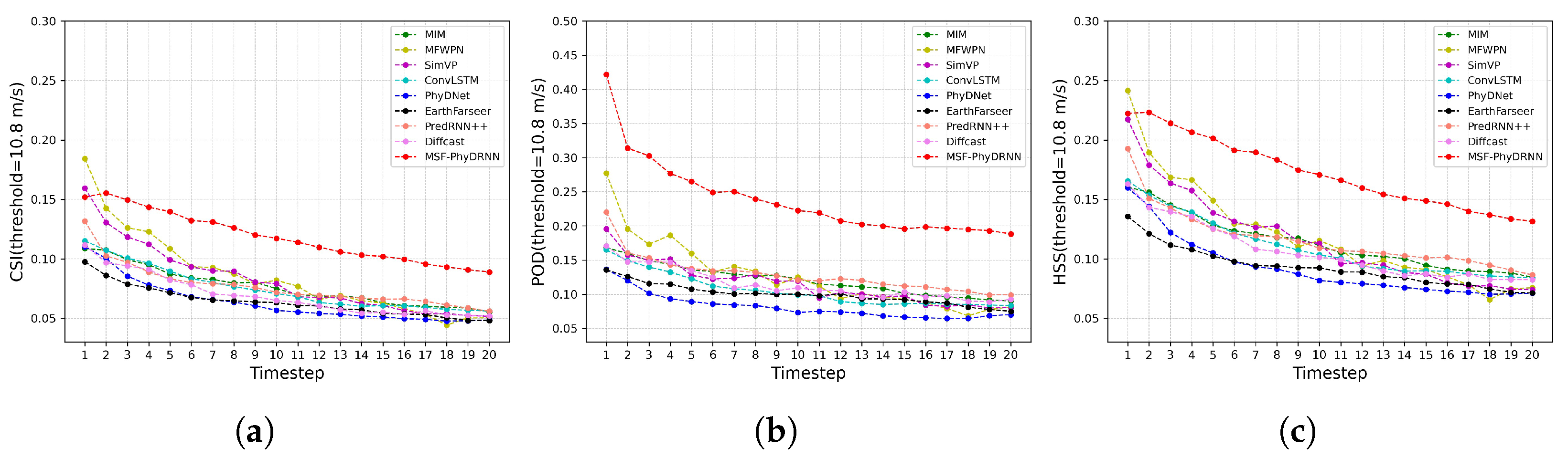
Figure 7 presents the trends of CSI, POD, and HSS for the proposed MSF-PhyDRNN and other advanced models on the Jiangsu dataset at a wind speed threshold of 10.8 m/s across successive prediction time steps. As indicated by the performance curves, the prediction accuracy of all models exhibits a consistent degradation trend as the forecast horizon extends, underscoring the inherent challenge of long-term severe wind speed prediction. Nevertheless, MSF-PhyDRNN demonstrates markedly superior performance compared to all benchmark models. In terms of POD, MSF-PhyDRNN achieves a significantly higher score at the initial steps and maintains this lead throughout the entire prediction range.

Among the baselines, the performances of ConvLSTM, MIM, and Diffcast are notably similar. Although PredRNN++ exhibits slightly lower CSI and HSS than ConvLSTM and MIM initially, it gradually outperforms them in later time steps. This improvement can be attributed to its incorporation of spatiotemporal LSTM units and gradient highway connections, which mitigate the vanishing gradient problem and enable more effective capture of dynamic evolution patterns. Despite its innovative CNN-Transformer hybrid architecture, MFWPN surpasses the other baselines only within the first eight time steps. Ultimately, while all baseline models suffer from severe progressive degradation over time, MSF-PhyDRNN exhibits exceptionally stable predictive performance, maintaining satisfactory results even in the later stages of the forecast horizon.

5. Ablation Study

To verify the effectiveness of the key components and the elaborately designed structure of our MSF-PhyDRNN model, we designed three controlled ablation configurations: (1) replacing the custom WMSE loss, which is tailored to thunderstorm gale speed thresholds and maximum values, with a standard MSE loss; (2) removing the multi-source data fusion module from the architecture; and (3) replacing the core SimplePredRNN++ recurrent unit with a standard ConvLSTM.

Table 4. Quantitative evaluation results of MSF-PhyDRNN and its variants on the Jiangsu dataset. The best scores are marked in bold.

Method	CSI			POD			SSIM	HSS
	1.6 m/s	5.5 m/s	10.8 m/s	1.6 m/s	5.5 m/s	10.8 m/s		1.6 m/s	5.5 m/s	10.8 m/s
PhyDNet	0.6531	0.3069	0.0635	0.7785	0.3888	0.0819	0.9707	0.6106	0.4284	0.0919
W/O WMSE	0.6649	0.3214	0.0755	0.7982	0.3907	0.1016	0.9734	0.6210	0.4423	0.1092
W/O MSF	0.6608	0.3270	0.0865	0.7882	0.4196	0.1493	0.9729	0.6178	0.4527	0.1295
W/O SimplePredRNN++	0.6467	0.3028	0.0881	0.7750	0.3698	0.1403	0.9704	0.6011	0.4226	0.1295
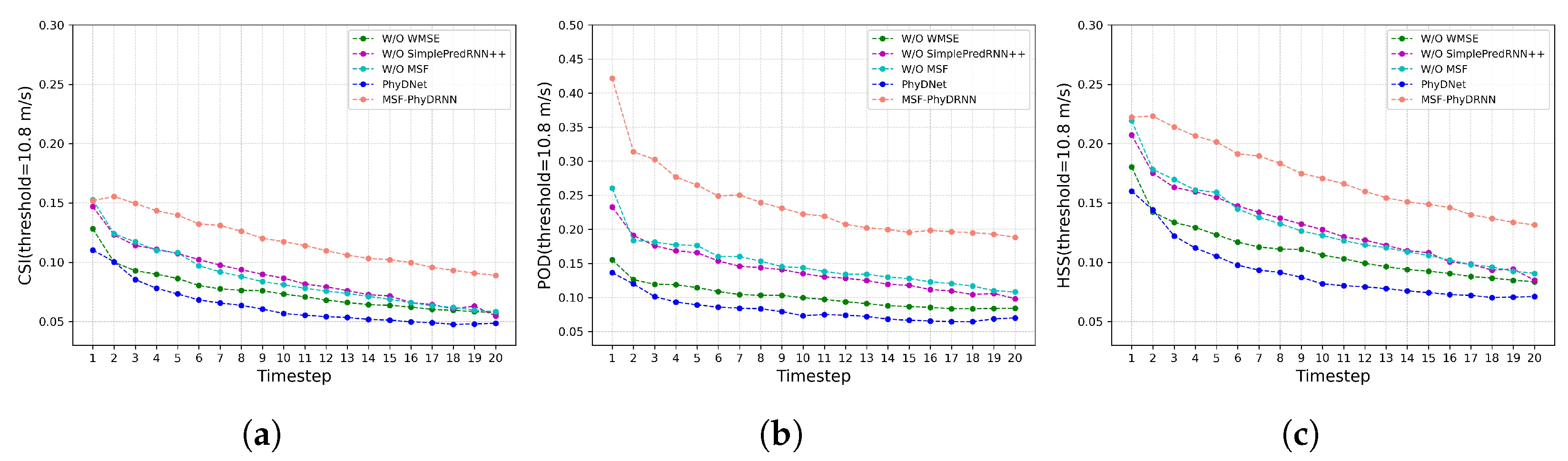
MSF-PhyDRNN	0.6709	0.3636	0.1185	0.8304	0.5149	0.2385	0.9742	0.6212	0.4947	0.1722

summarizes the 2-h prediction performance evaluated on the Jiangsu dataset. As indicated by the results, the proposed MSF-PhyDRNN achieves optimal performance in CSI, POD, HSS, and SSIM compared to its ablated variants. Notably, replacing the WMSE loss function with the standard MSE loss leads to the most significant declines in the CSI and POD metrics at the high threshold of 10.8 m/s. This validates the targeted optimization effect of the WMSE loss for predicting high-threshold thunderstorm gales. By assigning a higher weight to severe wind events, the WMSE loss enables the model to focus more precisely on strong wind regions, thereby reducing interference from low wind speeds and enhancing the learning of high-wind-speed features. Furthermore, Figure 8 demonstrates that the w/o MSF and w/o SimplePredRNN++ recurrent unit variants exhibit highly similar performance across all evaluation metrics at the 10.8 m/s threshold, both consistently outperforming the w/o WMSE variant. This indicates that the WMSE loss plays an irreplaceable core role in high-threshold thunderstorm gale prediction, while the MSF module and the SimplePredRNN++ recurrent unit further enhance the model’s overall performance through multi-source data fusion and advanced spatiotemporal sequence modeling, respectively. Crucially, the complete MSF-PhyDRNN significantly outperforms all ablated variants across the evaluated metrics. This confirms that the core components do not function in isolation; instead, they complement each other through collaborative optimization. Specifically, the WMSE loss ensures accuracy for high-threshold strong winds, the MSF module enhances multi-source information fusion, and the SimplePredRNN++ recurrent unit improves the stability of long-sequence modeling. The synergistic combination of these three components ultimately yields a substantial improvement in the model’s overall predictive performance, demonstrating the soundness and efficacy of the MSF-PhyDRNN architecture.

6. Conclusions

This study proposes MSF-PhyDRNN, a novel spatiotemporal nowcasting model for thunderstorm gales. To effectively integrate weather radar reflectivity data and surface wind field observations, we designed a multi-source data fusion module that captures spatiotemporal relationships between different data sources through feature decoupling and an adaptive fusion attention mechanism. Furthermore, we developed a lightweight variant of PredRNN++ and utilized it to replace the original ConvLSTM within the PhyDNet framework. This modification enhances the model’s capability to capture inherent long-term dependencies and the complex nonlinear evolution of convective systems while reducing computational redundancy. Additionally, to address class imbalance and the critical need for accurate predictions of extreme wind speeds, we introduced a weighted mean squared error (WMSE) loss function. This formulation directs the model to prioritize high-wind-speed regions. Experimental evaluations demonstrate that MSF-PhyDRNN excels in maintaining wind speed morphology, positional accuracy, and intensity distribution, exhibiting distinct advantages in predicting high-threshold wind speeds.

Despite these advancements, certain limitations remain. The model’s predictive performance is inherently constrained by the quality and resolution of the input data. Moreover, while it performs effectively for short-term forecasting (0–2 h), accurately predicting the initiation and dissipation of convective systems beyond this temporal window remains challenging. Additionally, although MSF-PhyDRNN demonstrates robust performance in the typical thunderstorm gale hotspots of South China and Jiangsu, its empirical validation in other geographic regions with distinct climatic characteristics is currently constrained by the limited availability of high-quality, paired radar and surface wind datasets. Future work will focus on incorporating dynamic physical constraint modules to enhance the model’s ability to simulate the complete life cycle of convective systems over extended forecast horizons. Furthermore, we plan to acquire diverse regional datasets to evaluate and optimize the model’s cross-regional generalizability utilizing transfer learning techniques.

References

1. Hoolohan, V.; Tomlin, A.S.; Cockerill, T. Improved near surface wind speed predictions using Gaussian process regression combined with numerical weather predictions and observed meteorological data. Renew. Energy 2018, 126, 1043–1054. [Google Scholar] [CrossRef] [Scilit]
2. Tang, X.Y.; Zhao, S.; Fan, B.; Peinke, J.; Stoevesandt, B. Micro-scale wind resource assessment in complex terrain based on CFD coupled measurement from multiple masts. Appl. Energy 2019, 238, 806–815. [Google Scholar] [CrossRef] [Scilit]
3. Yan, B.; Shen, R.; Li, K.; Wang, Z.; Yang, Q.; Zhou, X.; Zhang, L. Spatio-temporal correlation for simultaneous ultra-short-term wind speed prediction at multiple locations. Energy 2023, 284, 128418. [Google Scholar] [CrossRef] [Scilit]
4. Cai, H.; Jia, X.; Feng, J.; Li, W.; Hsu, Y.M.; Lee, J. Gaussian process regression for numerical wind speed prediction enhancement. Renew. Energy 2020, 146, 2112–2123. [Google Scholar] [CrossRef] [Scilit]
5. Erdem, E.; Shi, J. ARMA based approaches for forecasting the tuple of wind speed and direction. Appl. Energy 2011, 88, 1405–1414. [Google Scholar] [CrossRef] [Scilit]
6. Wang, J.; Hu, J. A robust combination approach for short-term wind speed forecasting and analysis—Combination of the ARIMA (Autoregressive Integrated Moving Average), ELM (Extreme Learning Machine), SVM (Support Vector Machine) and LSSVM (Least Square SVM) forecasts using a GPR (Gaussian Process Regression) model. Energy 2015, 93, 41–56. [Google Scholar] [CrossRef] [Scilit]
7. Shukur, O.B.; Lee, M.H. Daily wind speed forecasting through hybrid KF-ANN model based on ARIMA. Renew. Energy 2015, 76, 637–647. [Google Scholar] [CrossRef] [Scilit]
8. Aasim; Singh, S.; Mohapatra, A. Repeated wavelet transform based ARIMA model for very short-term wind speed forecasting. Renew. Energy 2019, 136, 758–768. [Google Scholar] [CrossRef] [Scilit]
9. Hill, D.C.; McMillan, D.; Bell, K.R.; Infield, D. Application of auto-regressive models to UK wind speed data for power system impact studies. IEEE Trans. Sustain. Energy 2011, 3, 134–141. [Google Scholar] [CrossRef] [Scilit]
10. Mohandes, M.A.; Halawani, T.O.; Rehman, S.; Hussain, A.A. Support vector machines for wind speed prediction. Renew. Energy 2004, 29, 939–947. [Google Scholar] [CrossRef] [Scilit]
11. Li, L.L.; Zhao, X.; Tseng, M.L.; Tan, R.R. Short-term wind power forecasting based on support vector machine with improved dragonfly algorithm. J. Clean. Prod. 2020, 242, 118447. [Google Scholar] [CrossRef] [Scilit]
12. Bhaskar, K.; Singh, S.N. AWNN-assisted wind power forecasting using feed-forward neural network. IEEE Trans. Sustain. Energy 2012, 3, 306–315. [Google Scholar] [CrossRef] [Scilit]
13. Kramer, O.; Gieseke, F. Short-term wind energy forecasting using support vector regression. In Proceedings of the Soft Computing Models in Industrial and Environmental Applications, 6th International Conference SOCO 2011; Springer: Berlin/Heidelberg, Germany, 2011; pp. 271–280. [Google Scholar] [CrossRef] [Scilit]
14. Khodayar, M.; Wang, J. Spatio-temporal graph deep neural network for short-term wind speed forecasting. IEEE Trans. Sustain. Energy 2018, 10, 670–681. [Google Scholar] [CrossRef] [Scilit]
15. Shi, X.; Chen, Z.; Wang, H.; Yeung, D.Y.; Wong, W.K.; Woo, W.C. Convolutional lstm network: A machine learning approach for precipitation nowcasting. In Advances in Neural Information Processing Systems; Curran Associates, Inc.: New York, NY, USA, 2015; Volume 28. [Google Scholar]
16. Duan, J.; Zuo, H.; Bai, Y.; Duan, J.; Chang, M.; Chen, B. Short-term wind speed forecasting using recurrent neural networks with error correction. Energy 2021, 217, 119397. [Google Scholar] [CrossRef] [Scilit]
17. Hochreiter, S.; Schmidhuber, J. Long short-term memory. Neural Comput. 1997, 9, 1735–1780. [Google Scholar] [CrossRef] [Scilit]
18. Chung, J.; Gulcehre, C.; Cho, K.; Bengio, Y. Empirical evaluation of gated recurrent neural networks on sequence modeling. arXiv 2014, arXiv:1412.3555. [Google Scholar] [CrossRef] [Scilit]
19. Farah, S.; Humaira, N.; Aneela, Z.; Steffen, E.; David A, W. Short-term multi-hour ahead country-wide wind power prediction for Germany using gated recurrent unit deep learning. Renew. Sustain. Energy Rev. 2022, 167, 112700. [Google Scholar] [CrossRef] [Scilit]
20. Wei, D.; Tian, Z. A comprehensive multivariate wind speed forecasting model utilizing deep learning neural networks. Arab. J. Sci. Eng. 2024, 49, 16809–16828. [Google Scholar] [CrossRef] [Scilit]
21. Yang, L.; Zhang, Z. A deep attention convolutional recurrent network assisted by k-shape clustering and enhanced memory for short term wind speed predictions. IEEE Trans. Sustain. Energy 2021, 13, 856–867. [Google Scholar] [CrossRef] [Scilit]
22. Ruan, Z.; Sun, W.; Yuan, Y.; Tan, H. Accurately forecasting solar radiation distribution at both spatial and temporal dimensions simultaneously with fully-convolutional deep neural network model. Renew. Sustain. Energy Rev. 2023, 184, 113528. [Google Scholar] [CrossRef] [Scilit]
23. Wang, J.; Lin, L.; Gao, S.; Zhang, Z. Deep generation network for multivariate spatio-temporal data based on separated attention. Inf. Sci. 2023, 633, 85–103. [Google Scholar] [CrossRef] [Scilit]
24. Lin, L.; Zhang, Z.; Yu, H.; Wang, J.; Gao, S.; Zhao, H.; Zhang, J. StHCFormer: A multivariate ocean weather predicting method based on spatiotemporal hybrid convolutional attention networks. IEEE J. Sel. Top. Appl. Earth Obs. Remote Sens. 2024, 17, 3600–3614. [Google Scholar] [CrossRef] [Scilit]
25. Wang, Y.; Jiang, L.; Yang, M. Eidetic 3D LSTM: A model for video prediction and beyond. In Proceedings of the International Conference on Learning Representations, Vancouver, BC, Canada, 30 April–3 May 2018; pp. 26–33. [Google Scholar]
26. Zhang, Z.; Lin, L.; Gao, S.; Wang, J.; Zhao, H.; Yu, H. A machine learning model for hub-height short-term wind speed prediction. Nat. Commun. 2025, 16, 3195. [Google Scholar] [CrossRef] [Scilit] [PubMed]
27. Wang, Y.; Gao, Z.; Long, M.; Wang, J.; Yu, P.S. Predrnn++: Towards a resolution of the deep-in-time dilemma in spatiotemporal predictive learning. In Proceedings of the International Conference on Machine Learning; PMLR: New York, NY, USA, 2018; pp. 5123–5132. [Google Scholar] [CrossRef] [Scilit]
28. Guen, V.L.; Thome, N. Disentangling physical dynamics from unknown factors for unsupervised video prediction. In Proceedings of the IEEE/CVF Conference on Computer Vision and Pattern Recognition; IEEE: Piscataway, NJ, USA, 2020; pp. 11474–11484. [Google Scholar] [CrossRef] [Scilit]
29. Association of American Geographers. Annals of the Association of American Geographers; Association of American Geographers: Washington, DC, USA, 1924; Volume 14. [Google Scholar]
30. He, K.; Zhang, X.; Ren, S.; Sun, J. Deep residual learning for image recognition. In Proceedings of the IEEE Conference on Computer Vision and Pattern Recognition; IEEE: Piscataway, NJ, USA, 2016; pp. 770–778. [Google Scholar] [CrossRef] [Scilit]
31. Woo, S.; Park, J.; Lee, J.Y.; Kweon, I.S. CBAM: Convolutional block attention module. In Proceedings of the European Conference on Computer Vision (ECCV); Springer: Cham, Switzerland, 2018; pp. 3–19. [Google Scholar] [CrossRef] [Scilit]
32. Wang, Y.; Zhang, J.; Zhu, H.; Long, M.; Wang, J.; Yu, P.S. Memory in memory: A predictive neural network for learning higher-order non-stationarity from spatiotemporal dynamics. In Proceedings of the IEEE/CVF Conference on Computer Vision and Pattern Recognition; IEEE: Piscataway, NJ, USA, 2019; pp. 9154–9162. [Google Scholar] [CrossRef] [Scilit]
33. Schaefer, J.T. The critical success index as an indicator of warning skill. Weather Forecast. 1990, 5, 570–575. [Google Scholar] [CrossRef] [Scilit]
34. Brotzge, J.A.; Nelson, S.E.; Thompson, R.L.; Smith, B.T. Tornado probability of detection and lead time as a function of convective mode and environmental parameters. Weather Forecast. 2013, 28, 1261–1276. [Google Scholar] [CrossRef] [Scilit]
35. Hogan, R.J.; Ferro, C.A.; Jolliffe, I.T.; Stephenson, D.B. Equitability revisited: Why the “equitable threat score” is not equitable. Weather Forecast. 2010, 25, 710–726. [Google Scholar] [CrossRef] [Scilit]
36. Han, D.; Choo, M.; Im, J.; Shin, Y.; Lee, J.; Jung, S. Precipitation nowcasting using ground radar data and simpler yet better video prediction deep learning. GISci. Remote Sens. 2023, 60, 2203363. [Google Scholar] [CrossRef] [Scilit]
37. Wu, H.; Liang, Y.; Xiong, W.; Zhou, Z.; Huang, W.; Wang, S.; Wang, K. Earthfarsser: Versatile spatio-temporal dynamical systems modeling in one model. Proc. AAAI Conf. Artif. Intell. 2024, 38, 15906–15914. [Google Scholar] [CrossRef] [Scilit]
38. Yu, D.; Li, X.; Ye, Y.; Zhang, B.; Luo, C.; Dai, K.; Wang, R.; Chen, X. Diffcast: A unified framework via residual diffusion for precipitation nowcasting. In Proceedings of the IEEE/CVF Conference on Computer Vision and Pattern Recognition; IEEE: Piscataway, NJ, USA, 2024; pp. 27758–27767. [Google Scholar] [CrossRef] [Scilit]
Figure 1. Visual correlation between S-band radar composite reflectivity and surface wind field.
Remotesensing 18 01334 g001
Figure 2. The overall architecture of MSF-PhyDRNN.
Remotesensing 18 01334 g002
Figure 3. The structure of the Multi-Source Fusion Module.
Remotesensing 18 01334 g003
Figure 4. The structure of the Simple PredRNN++ Recurrent Unit.
Remotesensing 18 01334 g004
Figure 5. Comparison of prediction results for two severe thunderstorm gale cases. Forecasted and observed wind speed comparisons over the Jiangsu dataset for 0–2 h wind speed predictions, visualized at two-timestep intervals. (a) Case I. A multi-cell cluster thunderstorm gale case. (b) Case II. A supercell thunderstorm gale case.
Remotesensing 18 01334 g005
Figure 6. Comparison of prediction results for a boundary layer convergence line thunderstorm gale case. 24-timestep prediction results on the South China Dataset, visualized at 3-timestep intervals.
Remotesensing 18 01334 g006
Figure 7. Comparative evaluation of CSI, POD, and HSS across different prediction time steps for the nine tested methods on the Jiangsu dataset. (a) CSI curve at the 10.8 m/s threshold. (b) POD curve at the 10.8 m/s threshold. (c) HSS curve at the 10.8 m/s threshold.
Remotesensing 18 01334 g007
Figure 8. Ablation study of CSI, POD, and HSS across different prediction time steps for MSF-PhyDRNN and its variants on the Jiangsu dataset. (a) CSI curve at the 10.8 m/s threshold. (b) POD curve at the 10.8 m/s threshold. (c) HSS curve at the 10.8 m/s threshold.
Remotesensing 18 01334 g008