Article

A Variational Random Finite-Set Approach to Highly Robust Active-Sonar Multi-Target Tracking Under Strong Reverberation

1
School of Marine Science and Technology, Northwestern Polytechnical University, Xi’an 710072, China
2
Shaanxi Key Laboratory of Underwater Information Technology, Xi’an 710072, China
3
Han Jiang National Laboratory, Xi’an Research Center, Xi’an 710072, China
4
Hai Ying Enterprise Group Co., Ltd., Wuxi 214028, China
*
Author to whom correspondence should be addressed.
Remote Sens. 2026, 18(9), 1332; https://doi.org/10.3390/rs18091332
Submission received: 7 March 2026 / Revised: 23 April 2026 / Accepted: 23 April 2026 / Published: 26 April 2026
(This article belongs to the Section Ocean Remote Sensing)

Highlights

What are the main findings?
  • We propose a robust Student’s t-distribution-based delta-Generalized Labeled Multi-Bernoulli (ST-δ-GLMB) filter. This filter addresses the non-stationary, non-Gaussian measurement noise in strong reverberation by using a variational Bayesian inference for online parameter estimation, significantly enhancing the tracking robustness in dynamic underwater environments.
  • We derive closed-form update and propagation rules for the Student’s t-distribution parameters within the GLMB framework. This innovation maintains manageable computational complexity and facilitates the practical implementation with minimal modifications to the existing systems.
What are the implications of the main findings?
  • Comprehensive validations using Monte Carlo simulations and real sea trial data demonstrate that the ST-δ-GLMB filter outperforms several state-of-the-art algorithms under strong reverberation. It effectively suppresses the increase in OSPA distance, reduces label switching errors, and maintains reliable trajectory continuity.
  • The proposed method achieves a stable estimation of the number of targets (cardinality) and exhibits superior performance in non-stationary noise conditions, which is crucial for dependable underwater multi-target surveillance applications.

Abstract

Active sonar tracking of multiple underwater targets is frequently challenged by intense reverberation, which leads to sonar returns that are both non-stationary and non-Gaussian. In such scenarios, the generalized labeled multi-Bernoulli (GLMB) filter, which relies on a Gaussian assumption, often experiences a rise in an Optimal Subpattern Assignment (OSPA) distance, along with recurrent label switching. To mitigate this problem, a robust delta-generalized labeled multi-Bernoulli technique (ST-δ-GLMB) is introduced; it characterizes noise using a Student’s t-distribution and employs variational Bayes to estimate the corresponding parameters. More precisely, the Student’s t-distribution is utilized to represent measurement non-stationarity, and an online variational Bayesian estimation of the noise parameters is conducted within a multi-target framework based on the Student’s t-model. Moreover, without altering the GLMB data-association and label-management machinery, we derive closed-form updates and propagation for the Student’s t-parameters, thereby keeping the recursive computational burden and practical implementability under control. Finally, Monte Carlo simulations and lake-trial data demonstrate that, under non-stationary and heavy-clutter conditions, ST-δ-GLMB maintains stable track continuity and accurate target-number (cardinality) estimates in the presence of non-stationary measurements.

1. Introduction

The localization and monitoring of submerged objects constitutes a vital field within subaqueous acoustic data analysis. Particularly, the active pursuit of multiple targets offers considerable utility in domains such as undersea combat defense and the investigation of oceanic resources [1,2,3,4]. However, in practice, reverberation in complex underwater environments causes measurements to exhibit non-stationary and non-Gaussian characteristics, degrading tracking performance. Thus, robust tracking under such conditions is an urgent research need.
The aim of multi-target tracking is to concurrently establish the number, conditions, and paths of targets within environments containing noise, undetected objects, spurious signals, and stochastic target appearance and disappearance [5]. Traditional methods, like Nearest Neighbor (NN) [6], Probability Data Association (PDA) [7], and Multiple Hypothesis Tracking (MHT) [8], rely on data association, assigning measurements to tracks at each time step. This paradigm typically lacks an explicit “target set” state variable and probabilistic cardinality (number of targets) modeling, managing target birth/death via thresholds and heuristics. This can lead to combinatorial explosion and high computational load, limiting scalability.
The Random Finite Set (RFS) framework overcomes these limitations by treating the target and measurement collections as set-valued variables, enabling rigorous Bayesian recursion via Finite Set Statistics (FISST) for joint cardinality and state estimation [9]. Notable advancements encompass the Probability Hypothesis Density (PHD) filter, a technique that disseminates the primary statistical moment for states involving multiple targets [9]. This filter has been realized through Gaussian Mixture (GM-PHD) [10] and Sequential Monte Carlo (SMC-PHD) [11] approaches. The Cardinalized PHD (CPHD) filter improved cardinality estimation accuracy by modeling its distribution explicitly [12], often implemented via GM or SMC [13,14]. However, PHD/CPHD filters do not maintain target identities, preventing continuous track labeling.
The Generalized Labeled Multi-Bernoulli (GLMB) method resolved this issue through the incorporation of unique markers, which permit the concurrent calculation of both the status and distinct identification of targets, thereby yielding enhanced results in challenging environments [15,16]. Its derivatives further enhanced its capabilities [17,18,19,20]. To reduce its computational burden, the δ-GLMB filter was proposed, using the Kronecker delta function to compress the posterior density representation while maintaining tracking performance and label consistency [21,22].
A common assumption in these filters is known as stationary noise statistics. Underwater reverberation violates this, presenting non-Gaussian, non-stationary measurement noise. To address uncertain noise, adaptive RFS filters have been developed. These include Variational Bayesian (VB)-based adaptive PHD [23,24] and CPHD [25] filters, Sage-Husa-based CPHD [26], and VB-integrated filters like the improved CBMeMBer [27], an LMB with Gaussian-Inverse Gamma form [28], and a δ-GLMB with Gaussian-Inverse Wishart implementation [29]. While enhancing adaptability, these methods predominantly rely on Gaussian conjugate priors, which may not fully capture the heavy-tailed, time-varying noise in active sonar, potentially causing increased OSPA distance and label swapping, undermining track continuity.
To better position the proposed method with respect to existing adaptive RFS filters, the main contributions of this paper are summarized as follows. First, unlike Gaussian adaptive-noise RFS filters, the proposed ST-δ-GLMB explicitly models heavy-tailed and time-varying measurement uncertainty using a Student’s t-likelihood, which improves the robustness of outliers and abrupt reverberation-induced clutter surges. Second, compared with VB-δ-GLMB, the proposed method combines Student’s t-noise modeling with online variational Bayesian parameter estimations within the δ-GLMB framework, thereby improving the resistance of the heavy-tailed interference and reducing label switching caused by noise mismatch during target birth/death and abrupt interference changes. Third, closed-form recursive updates are derived without changing the original δ-GLMB data-association and label-management mechanism, which preserves the practical implementability of the filter. Finally, both Monte Carlo simulations and lake-trial data are used to validate the effectiveness of the proposed method.

2. Student’s t-Active Underwater Multi-Target Tracking Model

This part presents the motion framework and the sensor observation framework utilized in tracking multiple underwater targets.

2.1. Underwater Multi-Target Kinematic Model

Within aquatic settings, objects often travel at a steady pace to conserve power and maintain a low profile. Moreover, there is often a considerable distance between the target and the sonar array. Therefore, we describe underwater targets using a uniform motion model.
Based on the above analysis, the target state is modeled as follows: Assume that at time step k, the bearing of the object with respect to the sonar array is θ k , and its range is r k . Consequently, the target’s condition at instant k can be expressed as:
x k T = ( r k , r ˙ k , θ k , θ ˙ k )
Given the preceding assumptions, the kinematic formulation for a target moving uniformly with respect to the sonar array is as follows:
x k = F k x k 1 + W k
In the equation, x k represents the one-step state prediction at time k , x k 1 is the state at time k – 1. Furthermore, the state transition matrix is expressed as F k = 1 T 0 1 0 0 0 0 0 0 0 0 1 T 0 1 , in which T denotes the temporal separation between measurement instances, and W k is the disturbance term caused by unknown underwater disturbances, which is characterized by a normal distribution having an average of 0 and a dispersion matrix of Q k .

2.2. Underwater Active Tracking Measurement Model

Following preprocessing, the return signal from an active sonar system provides the target’s angle θ and distance r data. The measurement formula is as follows:
z k = H x k 1 + n k
The signal returns acquired through an active sonar setup typically include interference generated by ambient conditions like oceanic plankton, air pockets, and reflections from the sea floor. This study presumes that such interference exhibits a uniform spread across the monitored region and adheres to a Poisson point model.
To conclude, the operational sonar return measurement framework incorporates both the reflected pulses from genuine objects and the influence of significant interference. The real measurement collection is represented as:
Z k = { z k i : i = 1 N k } Clutter k
Here, Z k denotes the quantity of measurement returns from targets at time k step, while Clutter k corresponds to the set of clutter measurements.

3. δ-Generalized Labeled Multi-Bernoulli (δ-GLMB) Filter

For clarity, the main notations used in the δ-GLMB recursion and the variational Bayesian derivation are summarized in Table 1.
Within the mathematical expressions of the generalized labeled multi-Bernoulli filter, a lowercase letter (e.g., x or x ) denotes a single-target state. Conversely, a multi-target state is indicated by an uppercase letter. Furthermore, a labeled distribution is signified using bold characters, for example, x , X , and π , while uppercase symbols are used to emphasize sets or spaces, etc., such as X , Z , and L . Generally, matrices are represented by uppercase italic letters, such as H . The following formulation of the labeled random finite set and the δ--GLMB recursion follows the standard framework in [22,27].
At time k , a random finite set can represent the multi-target state and observations,
X k = { x k , 1 , x k , N ( k ) } X , Z k = { z k , 1 , z k , N ( k ) } Z
A labeled random finite set is characterized over the Cartesian product formed by the state domain X and the labeling domain L . Let the mapping L : X × L L be represented as L ( x , l ) = l , then for a labeled RFS X X × L , L ( X ) = { L ( x ) : x X } , this denotes the collection of every tag assigned to constituents within this labelled RFS. Only when the cardinality of the label set equals that of the RFS itself, that is, | L ( X ) | = | X | , can it be guaranteed that each sample element has a unique and different label. The ‘label uniqueness’ indicator function is introduced by the following formula:
Δ ( X ) δ | X | ( | L ( X ) | )
Here,
δ Y ( X ) { 1 , if   X = Y 0 , otherwise
While the Generalized Labeled Multi-Bernoulli (GLMB) distribution can be formulated to remain mathematically closed under Bayesian recursion, its concise representation typically requires summing across every possible subset of labels—a procedure that poses direct numerical implementation challenges. An alternative, fully equivalent formulation known as the δ-GLMB offers a solution:
π ( X ) = Δ ( X ) ( I , ξ ) F ( L ) × Ξ ω ( I , ξ ) δ I ( L ( X ) ) p ( ξ ) X
By setting ω ( I , ξ ) = ω ( ξ ) ( I ) , the “mixture” representation of GLMB is converted to a δ-function form, which yields a nonzero value solely under precise correspondence between the labeled sets, thus significantly streamlining the practical execution.

3.1. δ-GLMB Update

For the initial multi-target prior in the δ-GLMB filter, define the potential collection for the label space at the initial time 0 step as F ( L 0 ) , this yields the following:
π 0 ( X ) = Δ ( X ) I F ( L 0 ) ω 0 ( I ) δ I ( L ( X ) ) p 0 X
In this context, each I F ( L 0 ) denotes the collection of track identifiers originating at time 0; ω 0 ( I ) corresponds to the hypothesized weighting for the proposition that “the initial label set is I ”. Furthermore, for a given identifier l I , p 0 ( , l ) signifies the likelihood density function for the track’s starting kinematic condition.
In the δ-GLMB framework, the filtering and prediction distribution, which is revised using the measurement sequence Z 1 : k , can employ the association mapping history space Θ 0 : k Θ 0 × × Θ k as its discrete parameter domain Ξ . Here, Θ t denotes the collection of assignments linking measurements to tracks at time t step. Consequently, the revised distribution for the present moment is given by:
π ( X | Z ) = Δ ( X ) ( I , ξ ) F ( L ) × Ξ θ Θ ( I ) ω ( I , ξ , θ ) ( Z ) δ I ( L ( X ) ) p k ( ξ , θ ) ( | Z k ) X
Given the predicted δ-GLMB density π = I ( h ) , ξ ( h ) , ω ( h ) , p ( h ) h = 1 H , its update density Formula (10) can be decomposed as:
π ( X | Z ) = h = 1 H π ( h ) ( X | Z )
Here,
π ( h ) ( X | Z ) = Δ ( X ) j = 1 Θ I ( h ) ω ( h , j ) δ I ( h ) ( L ( X ) ) p ( h , j ) X
ω ( h , j ) ω I ( h ) , ξ ( h ) , θ ( h , j ) ( Z )
p ( h , j ) p { ξ ( h ) , θ ( h , j ) } ( | Z )
Every forecasting module h produces Θ I ( h ) , a set of candidate hypotheses. To maintain processing speed, these sets h must be pruned, ensuring just the necessary quantity of candidates remain.
To truncate the filter distribution π ( X | Z ) , first construct the cost matrix C z ( I ( h ) , ξ ( h ) ) and the assignment matrix S . Input the assignment matrix and the cost matrix into the optimal sorting method to obtain the top T ( h ) hypotheses θ ( h , 1 ) , , θ ( h , T ( h ) ) with weights from largest to smallest.

3.2. δ-GLMB Prediction

Based on the standard δ-GLMB prediction recursion in [21,22], the predicted multi-target density at the next time step can be expressed as follows:
π + ( X + ) = Δ ( X + ) ( I , ξ ) F ( L ) × Ξ ω ( I , ξ ) J F ( I ) η S ( ξ ) J 1 η S ( ξ ) I J L F ( B ) ω B ( L ) δ J L ( L ( X + ) ) p + ( ξ ) X +
Considering the revised δ-GLMB distribution π ( | Z ) for the present moment along with its listed set of parameters:
I ( h ) , ξ ( h ) , ω ( h ) , p ( h ) h = 1 H
The prediction for the δ-GLMB filter, presented in Equation (15) is expressible as an aggregate of multiple constituent parts:
π + ( X + ) = h = 1 H π + ( h ) ( X + )
where
π + ( h ) ( X + ) = Δ ( X + ) J I ( h ) ω S ( I ( h ) , ξ ( h ) ) ( J ) J B ω B ( L ) δ J L ( L ( X + ) ) p + ξ ( h ) X +
Mirroring the correction phase, considerations of computational performance and practical execution require the forecast distribution π + to be effectively approximated.
To model newly appearing targets, the labeled multi-Bernoulli approach is employed as follows:
ω B ( L ) = l B 1 r B ( l ) l L r B ( l ) 1 r B ( l )
p B ( x , l ) = p B ( l ) ( x )
Define a cost vector C B = [ C B ( l 1 ) , , C B ( l | B | ) ] on the birth label set B . Similarly, obtain the top K B birth subsets.
Combine the subsets obtained from the above two truncation steps and retain the top T = h = 1 H K ( h ) K B components. The truncated form for the h-th component is obtained:
π ^ + ( h ) ( X + ) = Δ ( X + ) j = 1 K ( h ) b = 1 K B ω + ( h , j , b ) δ j ( h , j ) L ( b ) ( L ( X + ) ) p + ( h ) X +
where
ω + ( h , j , b ) = ω S ( I ( h ) , ξ ( h ) ) J ( h , j ) ω B ( L ( b ) )
p + ( h ) = p + ξ ( h ) with   p + ξ ( h )   given   by :
p + ( h ) ( x , l ) = 1 L ( l ) i = 1 J ( ξ ) ( l ) ω i ( ξ ) ( l ) N x ; m S , i ( ξ ) ( l ) , P S , i ( ξ ) ( l ) + 1 B ( l ) p B ( l ) ( x )
where
m S , i ( ξ ) ( l ) = F m i ( ξ ) ( l )
P S , i ( ξ ) ( l ) = Q + F P i ( ξ ) ( l ) F T
The birth density p B ( l ) ( x )   is represented using a Gaussian mixture model. Correspondingly, after performing the corresponding truncation-prediction operation for all hypotheses h = 1 , , H   , normalization is applied to complete the distribution prediction.

3.3. δ-GLMB Multi-Target State Estimation

Derive the MAP cardinality approximation using the frequency distribution of set sizes:
N ^ : = arg max n ρ ( n )
where
ρ ( n ) = ( I , ξ ) F ( L ) × Ξ ω ( I , ξ ) δ n ( | I | )
Then, from all hypotheses, select the one with the same cardinality as N ^ and the largest weight, denoted by ( I ^ , ξ ^ ) , and then perform mean estimations for each label l I :
x ^ l = y p ξ ^ ( y , l ) d y

4. Robust Active Multi-Target Underwater Tracking Algorithm

4.1. Variational Bayesian Derivation Based on the Student’s t-Model

In order to obtain an analytical approximation to the posterior probability density function for a linear dynamical system with time-varying measurement disturbances, it is necessary to specify both the one-step predictive density p ( x k | z 1 : k 1 ) and the likelihood function p ( z k | x k ) . To model non-stationary and heavy-tailed measurement noise, we adopt the Student’s t-distribution and its hierarchical Gaussian-Gamma representation as in [15,30]. Accordingly, the measurement noise is modeled by a Student’s t-distribution as follows:
  p ( v k ) = S t ( v k ; 0 , R k , v )
where S t ( v k ; 0 , R k , v ) denotes the Student’s t-probability density function with mean 0, scale matrix R k , and degrees of freedom v . The likelihood function can then be expressed as:
p ( z k | x k ) = S t ( z k ; H k x k , R k , v )
An exact analytical expression for the posterior probability density function in state-space models utilizing the Student’s t-distribution does not exist. To overcome this limitation, a supplementary stochastic variable is incorporated, transforming the Student’s t state-space framework into one that is Gaussian. This conversion is feasible because the Student’s t PDF can be expressed as a Gaussian mixture of unbounded order, allowing the preceding formula to be reformulated as:
p ( z k | x k ) = N ( z k ; H k x k , R k / λ k ) G λ k ; v 2 , v 2 d λ k
Here, the Gamma distribution G ( ; α , β ) is characterized by a shape parameter α and a rate parameter β . As a result, the likelihood can be formulated as follows:
p ( z k | x k , λ k ) = N ( z k ; H k x k , R k / λ k )
p ( λ k ) = G λ k , v 2 , v 2
Here, the state-space model is converted into a Gaussian hierarchical form. To jointly approximate the posterior distributions of the system state x k and the auxiliary latent variable λ k , we employ a variational Bayesian inference under the standard mean-field assumption following [26,30]. Accordingly, the joint posterior probability density function is approximated in the following factorized form:
p ( x k , λ k | z 1 : k ) q ( x k ) q ( λ k )
where q ( ) denotes the approximate posterior probability density function. The corresponding variational solution is obtained by minimizing the Kullback–Leibler divergence between the approximate posterior and the true posterior distribution:
{ q ( x k ) , q ( λ k ) } = arg min KLD q ( x k ) q ( λ k ) p ( x k , λ k | z 1 : k )
where
KLD q ( x ) p ( x ) q ( x ) log q ( x ) p ( x ) d x
The ideal outcome meets the following condition:
log q * ( λ k ) = E x log p ( x k , λ k , z 1 : k ) + c λ
log q * ( x k ) = E λ log p ( x k , λ k , z 1 : k ) + c x
where c ζ denotes a constant independent of ζ , and E ρ [ ρ ] represents the expectation of ρ . The joint probability density function p ( x k , λ k , z 1 : k ) is expressed as:
p ( x k , λ k , z 1 : k ) = p ( z k | x k , λ k ) p ( x k | z 1 : k 1 ) p ( λ k ) = N ( z k ; H k x k , R k / λ k ) N ( x k ; x ^ k | k 1 , P k | k 1 ) G λ k ; ν 2 , ν 2
Consequently, the optimal approximate posterior of λ k at the (i + 1)-th iteration is given by:
log q ( i + 1 ) ( λ k ) = m + ν 2 1 log λ k 0.5 { ν + Φ } + c λ
where
Φ = ( z k H k x ¯ k ) T R k 1 ( z k H k x ¯ k ) T + tr R k 1 H k P k | k 1 H k T
Using the above equation, q ( i + 1 ) ( λ k ) is updated as a Gamma PDF:
q ( i + 1 ) ( λ k ) = G λ k ; γ k i + 1 , δ k i + 1
where
γ k i + 1 = m + ν 2
δ k i + 1 = ν + Φ 2
Similarly, the optimal approximate posterior for   x k at the (i + 1)-th iteration is given by:
log q ( i + 1 ) ( x k ) = 0.5 E i + 1 ( λ k ) ( z k H k x k ) T R k 1 ( z k H k x k ) T   0.5 ( x k x ^ k | k 1 ) T P k | k 1 1 ( x k x ^ k | k 1 ) + c x   = 0.5 x k T P k | k 1 1 + H k T R k / E i + 1 ( λ k ) 1 H k x k   + x k T P k | k 1 1 x ^ k | k 1 + H k T R k / E i + 1 ( λ k ) 1 z k + c x
At this point, q ( i + 1 ) ( x k )   is updated as a Gaussian distribution:
q ( i + 1 ) ( x k ) = N x k ; x k | k ( i + 1 ) , P k | k ( i + 1 )
where
x k | k ( i + 1 ) = P k | k 1 1 + H k T R ˜ k 1 H k 1 P k | k 1 1 x ^ k | k 1 + H T R ˜ k 1 z k   = P k | k 1 P k | k 1 H k T R ˜ k + H k P k | k 1 H k T 1 H k P k | k 1 P k | k 1 1 x ^ k | k 1 + H T R ˜ k 1 z k   = P k | k 1 K k H k P k | k 1 P k | k 1 1 x ^ k | k 1 + H T R ˜ k 1 z k   = x ^ k | k 1 + P k | k 1 H T R ˜ k 1 z k K k H k x ^ k | k 1 K k H k P k | k 1 H T R ˜ k 1 z k   = x ^ k | k 1 + K k z k H k x ^ k | k 1
P k | k ( i + 1 ) = P k | k 1 1 + H T R ˜ k H
R ˜ k = R k / E i + 1 ( λ k )
After N fixed-point iterations, the approximate posterior PDF is updated as:
q N ( λ k ) = G ( λ k ; γ k N , δ k N )
q N ( x k ) = N ( x k ; x k | k N , P k | k N )

4.2. A Robust Tracking Method Based on Variational Random Finite Sets

Combining the variational Bayesian derivation process given above, after undergoing N iterations, Equations (22)–(25) can be rewritten as:
q i ( ξ ( h ) ) ( z ; l ) = N z ; H m i ( ξ ( h ) ) ( l ) , H P i ( ξ ( h ) ) N ( l ) H T + R ˜ k
m Z , i ( ξ ( h ) , θ ( h , j ) ) ( l ) = m i ( ξ ( h ) ) ( l ) + K i ( ξ ( h ) , θ ( h , j ) ) ( l ) z θ ( l ) H m i ( ξ ( h ) ) ( l ) if   θ ( h , j ) ( l ) > 0 m i ( ξ ( h ) ) ( l ) if   θ ( h , j ) ( l ) = 0
P i ( ξ ( h ) , θ ( h , j ) ) ( l ) = I K i ( ξ ( h ) , θ ( h , j ) ) ( l ) H P i ( ξ ( h ) ) ( l ) N
K i ( ξ ( h ) , θ ( h , j ) ) ( l ) = P i ( ξ ( h ) ) ( l ) H T H P i ( ξ ( h ) ) ( l ) N H T + R ˜ k 1 if   θ ( h , j ) ( l ) > 0 0 if   θ ( h , j ) ( l ) = 0
Based on the above theory, the complete procedure of the ST-δ-GLMB filter is presented. The procedure for a single iteration of the presented method is illustrated in Algorithm 1.
Algorithm 1. ST-δ-GLMB Filter Procedure
Main Loop:
Prediction:
For   k = 1 : K :
Input:   { ( I ( h ) , ξ ( h ) , ω ( h ) , p ( h ) , K ( h ) ) } h = 1 H , K B , { ( r B ( l ) , P B ( l ) ) } l B
Calculate the birth hypothesis cost matrix C B
{ L ( b ) } b = 1 K B : = k _ s h o r t e s t _ p a t h ( B , C B , K B )
For b = 1 : K B :
ω B ( b ) : = l L ( b ) r B ( l ) l B L b 1 r B ( l )
End
For h = 1 : H :
η S ( h ) : = η S ( ξ ( h ) )
C S ( h ) : = C S ( I ( h ) , ξ ( h ) )
{ J ( h , j ) } j = 1 K ( h ) : = k _ s h o r t e s t _ p a t h I ( h ) , C S ( h ) , T ( h )
For ( j , b ) = ( 1 , 1 ) : K ( h ) , K B :
I + ( h , j , b ) : = J ( h , j ) L ( b )
ω + ( h , j , b ) : = ω ( h ) η S ( h ) J ( h , j ) 1 η S ( h ) I ( h ) J ( h , j ) ω B ( b )
End
p + ( h ) : = p + ( ξ ( h ) ) can be calculated using Equation (23)
End
Normalize the weights: ω + ( h , j , b ) ( h , j , b ) = ( 1 , 1 , 1 ) ( H , K ( h ) , K B )
Output: I + ( h , j , b ) , ω + ( h , j , b ) , P ( h ) ( h , j , b ) = ( 1 , 1 , 1 ) ( H , K ( h ) , K B )
Update:
1. Input :   I ( h ) , ξ ( h ) , ω ( h ) , P ( h ) , T ( h ) h = 1 H , Z
2. For   h = 1 : H
3. C Z ( h ) : = C Z I ( h ) , ξ ( h )
4. θ ( h , j ) j = 1 T ( h ) : = r a n k _ a s s i g n m e n t ( Z , I ( h ) , C Z ( h ) , T ( h ) )
5. For   j = 1 : T ( h )
For   n = 1 : N (Variational Bayesian iteration)
6. η Z ( h , j ) : = η Z ( ξ ( h ) , θ ( h , j ) ) n , Calculate using Equation (19) combined with Equations (52)–(55)
p ( h , j ) : = ( p ( ξ ( h ) , θ ( h , j ) ) ( | Z ) ) n , Calculate using Equation (20) combined with Equations (52)–(55)
7. End
8. ω ( h , j ) : = ω ( h ) η Z ( h , j ) I ( h )
9. I ( h , j ) : = I ( h )
10. ξ ( h , j ) : = ξ ( h ) , θ ( h , j )
11. End
12. End
13. Normalize   weights :   ω ( h , j ) ( h , j ) = ( 1 , 1 ) ( H , T ( h ) )
14. Output :   I ( h , j ) , ξ ( h , j ) , ω ( h , j ) , P ( h , j ) , T ( h , j ) ( h , j ) = ( 1 , 1 ) ( H , T ( h ) )
State Estimation:
Input:
I ( h , j ) , ξ ( h , j ) , ω ( h , j ) , P ( h , j ) , T ( h , j ) ( h , j ) = ( 1 , 1 ) ( H , T ( h ) ) , N max
ρ ( n ) : = h = 1 H j = 1 T ( h ) ω ( h , j ) δ n I ( h , j )
N ^ : = arg max n ρ ( n )
( h ^ , j ^ ) = arg max ( h , j ) ω ( h , j ) δ N ^ I ( h , j )
X ^ : = ( x , l ) : l I ( h ^ , j ^ ) , x y p ( h ^ , j ^ ) ( y , l ) d y
Output: X ^

5. Simulation Experiments and Analysis

To assess the resilience of the introduced δ-GLMB filtering method under conditions of extended-distance object tracking, a simulated study was constructed using a two-dimensional polar coordinate framework. The objects are situated across an angular span [0°, 180°] and a radial span from 1200 to 3000 m. The simulation duration is set to K = 150 time steps. Targets move along fixed-angle straight lines at different velocities, and the number of targets varies over time, including birth and death processes. An additional objective is positioned at the extreme right side to emulate a scenario with few targets, thereby examining its effect on filter operation.
The desired condition is characterized by radial coordinates and rotational speed: x k = ( r k , r ˙ k , θ k , θ ˙ k ) . Furthermore, the measurements are provided in polar coordinates: z k = ( r k , θ k ) . A constant-speed kinematic model, detailed in Equation (2), is employed for the target.
The measurement noise is modeled as:
V k = S T ( 0 , R , 5 ) with   probability   0.9 S T ( 0 , 100 R , 5 ) with   probability   0.1 ,
Here, the Student’s t-distribution S T ( m , Σ , v ) is represented, characterized by a specified mean m , a scale parameter Σ , and v degrees of freedom. The scale parameter is given by: R = 0.6 0 0 60 . The survival likelihood for the target is established at P s = 0.98 , with the detection chance set to P d = 0.90 . False alarms arise from a Poisson model, producing about 10 spurious measurements each time step. False alarms are generated according to a Poisson model. For the filter implementation, the number of updated and posterior hypotheses is both set to 1500, the hypothesis pruning threshold is set to 10 15 , and the VB update uses five fixed-point iterations at each time step. These settings are adopted to provide a challenging simulation scenario under strong clutter and non-stationary interference. The resulting target spatial arrangement appears in Figure 1.
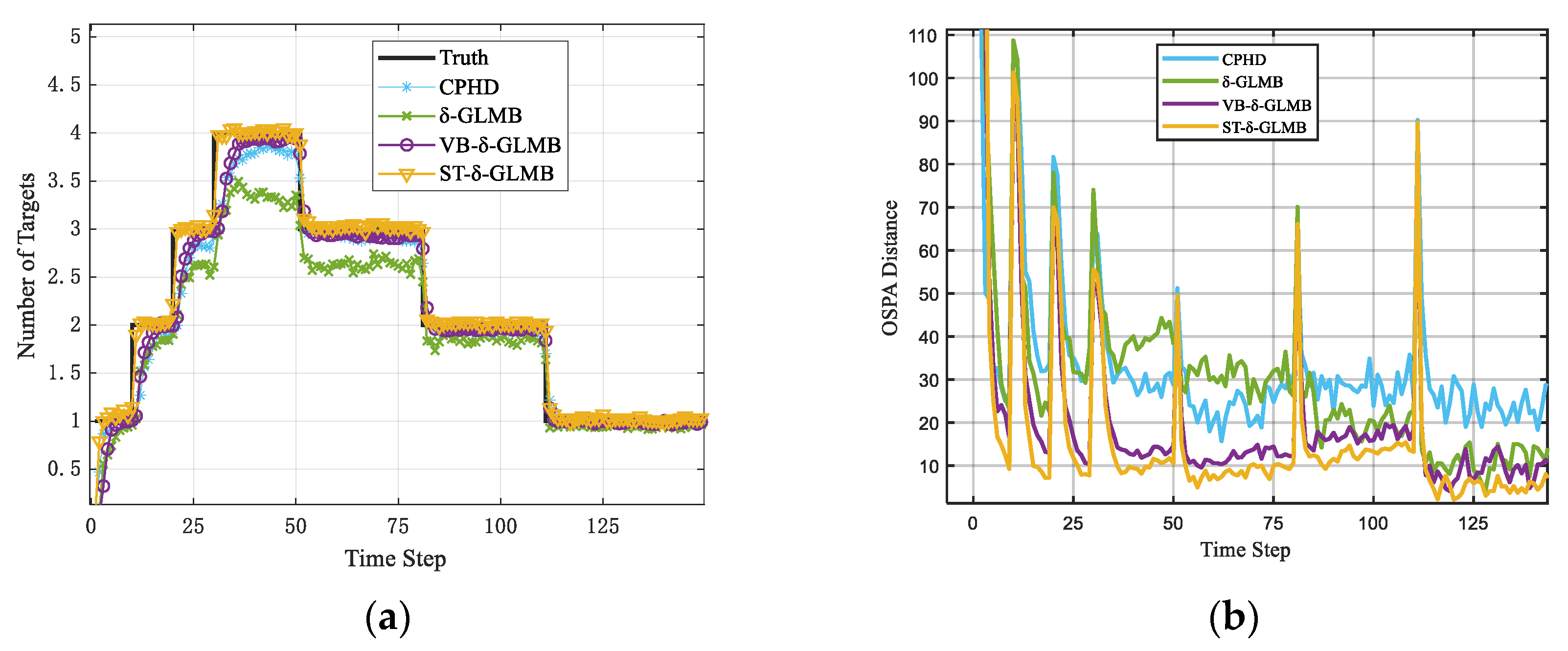
The proposed algorithm ST-δ-GLMB, along with the CPHD [10], δ-GLMB [20], and VB-δ-GLMB [27] filterswere run under identical conditions. Each simulation was independently repeated 200 times using the Monte Carlo method, and a comparative evaluation was performed using the OSPA metric, including both the cardinality error and OSPA distance. Figure 2 presents the outcomes of the experiment. To assess these findings quantitatively, Table 1 provides the RMSE for the quantity of targets and the mean OSPA metric.
Figure 2a displays the temporal variation in the estimated target quantities for four approaches, CPHD, δ-GLMB, VB-δ-GLMB, and ST-δ-GLMB, where a black line denotes the actual target quantity. These findings demonstrate that the CPHD method persistently produces lower target estimates than the true value across the whole duration, especially at moments when the target number changes abruptly, and only in the stable interval of “a single target existing for a long time” does it closely follow the true value. δ-GLMB can provide relatively accurate cardinality estimates in most periods, with a particularly stable performance in the 80–150 time step interval—where only two widely spaced targets exist, and measurement interference is weak—but a slight lag or overshoot is still observable during abrupt changes. VB-δ-GLMB and ST-δ-GLMB overall show high consistency with the true values. However, VB-δ-GLMB exhibits a brief decrease in accuracy at the moment of target number transition, which is due to its adaptive adjustment of the noise covariance for each measurement, tending to over-smooth abrupt changes, and thus weakening its sensitivity to rapid environmental changes. In contrast, ST-δ-GLMB not only maintains the agile response of δ-GLMB at change points but also significantly improves the stability and accuracy of estimation throughout the entire process. This improvement is likely due to the joint effect of three factors. First, the Student’s t-measurement model is more tolerant to heavy-tailed outliers and abrupt reverberation-induced interference than Gaussian modeling. Second, the variational Bayesian update enables online adaptations of the noise parameters, which improves robustness to time-varying measurement statistics. Third, because these updates are embedded within the δ-GLMB framework without changing its original data-association and label-management mechanism, the filter preserves track continuity more effectively during target birth/death events and abrupt interference changes.
Figure 2b shows the average OSPA over time for each method. The CPHD method exhibits a markedly greater OSPA magnitude compared to alternative approaches, characterized by distinct peaks and a gradual return to baseline over the fluctuation range; this behavior often leads to trajectory termination or erroneous prolongation. The three GLMB-based methods generally have significantly lower errors. However, δ-GLMB does not explicitly handle non-stationary measurement noise, leading to a sustained increase in OSPA when measurement statistics change or target interaction intensifies. VB-δ-GLMB effectively alleviates this problem through parameter adaptation, further reducing both spike amplitude and steady-state error. ST-δ-GLMB maintains the lowest and smoothest OSPA curve throughout the entire period, with the smallest spike amplitude and the shortest recovery duration at the birth/death moments. This result is consistent with its stronger robustness to heavy-tailed interference, improved adaptation to time-varying measurement statistics, and better preservation of track continuity within the δ-GLMB framework.
From Table 2, it can be seen that the quantitative results are consistent with the above observations. In terms of the RMSE of the target number, CPHD, δ-GLMB, VB-δ-GLMB, and ST-δ-GLMB are 1.37, 0.41, 0.29, and 0.13, respectively. Compared to the best-performing VB-δ-GLMB, ST-δ-GLMB reduces the error by 55.2%. Regarding the average OSPA, the four methods yield 46.80, 32.41, 20.72, and 18.53, respectively. ST-δ-GLMB shows a 10.6% reduction compared to VB-δ-GLMB. Overall, ST-δ-GLMB achieves the best performance in both cardinality estimation and geometric error metrics under the considered simulation setting, and shows stronger robustness in scenarios with abrupt target-number changes and time-varying measurement interference.
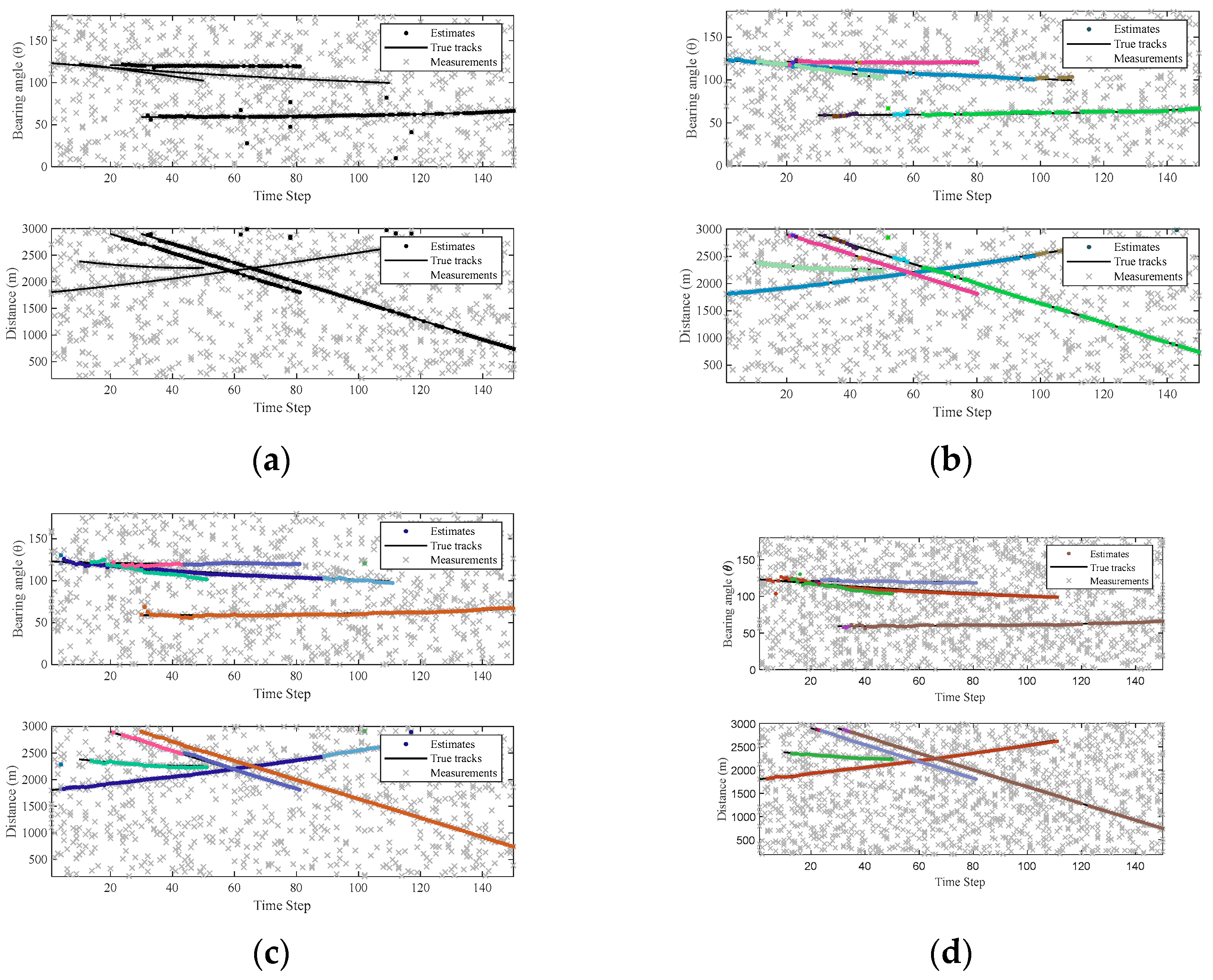
Furthermore, to better clarify the principles underlying Figure 2, a specific tracking result of the four tracking algorithms is presented in Figure 3 for combined illustration. In Figure 3a, we can see that the CPHD method not only performs poorly in tracking accuracy compared to GLMB-based methods but, more importantly, unlike GLMB, it does not provide target trajectory information, which is reflected in the figure as the accumulation of points obtained at different times.
As illustrated in Figure 3b, the δ-GLMB filter delivers superior tracking accuracy relative to the CPHD method and additionally generates well-defined trajectories for individual targets. Nonetheless, the green path in the diagram indicates that performance can be affected during transitions in the target count (such as those occurring around time steps 50 and 70) or when the measurement noise suddenly becomes abnormal, the trajectory may break. This is due to the inability of GLMB to adapt to non-stationary measurement noise.
In Figure 3c, we can see that the tracking result of the VB-δ-GLMB algorithm appears visually good and has a better ability to adapt to non-stationary noise. However, after the trajectory stabilizes in the figure, its label suddenly changes; one trajectory appears in two colors. This is because the VB with the Gaussian modeling cannot adapt to severe changes in measurement noise, leading to label switching in continuous trajectories. Conversely, Figure 3d demonstrates that the introduced ST-δ-GLMB filter is capable of adjusting to time-varying noise, and even if the trajectory breaks, the identity label does not switch when the target reappears.
To further quantitatively evaluate the label continuity and computational cost of different algorithms, Table 3 reports the average label switch count and the average runtime of the three methods. Here, the average label switch count is obtained from Monte Carlo simulations with four targets, and it reflects the frequency of label changes along the true target trajectories during the entire tracking process. To some extent, this metric also captures the influence of clutter interference, abnormal measurements, and target birth/death events on label stability. It can be seen that the average label switch counts of δ-GLMB, VB-δ-GLMB, and ST-δ-GLMB are 18.7, 12.5, and 7.8, respectively. Among them, ST-δ-GLMB yields the smallest number of label switches, indicating that it has the strongest label-maintenance capability under strong reverberation and non-stationary noise conditions, which is consistent with the qualitative observations in Figure 3.
In terms of runtime, the average runtimes of δ-GLMB, VB-δ-GLMB, and ST-δ-GLMB are 16.34 s, 18.27 s, and 19.03 s, respectively. It can be observed that the introduction of adaptive noise estimation and Student’s t-modeling leads to a certain increase in computational cost, with ST-δ-GLMB having the highest runtime among the three methods. However, the overall increase remains limited. Compared with the clear improvement achieved in label continuity and robustness, this additional computational burden is acceptable. Therefore, ST-δ-GLMB achieves better label consistency and stronger robustness against non-stationary noise while still maintaining good practical implementability.

6. Lake-Trial Data Validation and Analysis

6.1. Test Description

The ST-δ-GLMB method was verified using 2023 sonar measurements obtained from a Chinese lake. In the experiment, a ship was used to tow a cylindrical iron bucket to simulate an underwater vehicle, and a counterweight device was designed to allow the target to sink into the water. The cylindrical iron container was towed through the water, maintaining an operational depth of 10 m and a velocity of 0.5 m per second over a period of 90 s.
Signals were emitted using a directional acoustic emitter positioned 5 m below the surface. The outgoing waveform was an HFM type, featuring a central frequency between 32 kHz and 35 kHz, a 0.1 s pulse duration, and a 1 s interval between pulses.
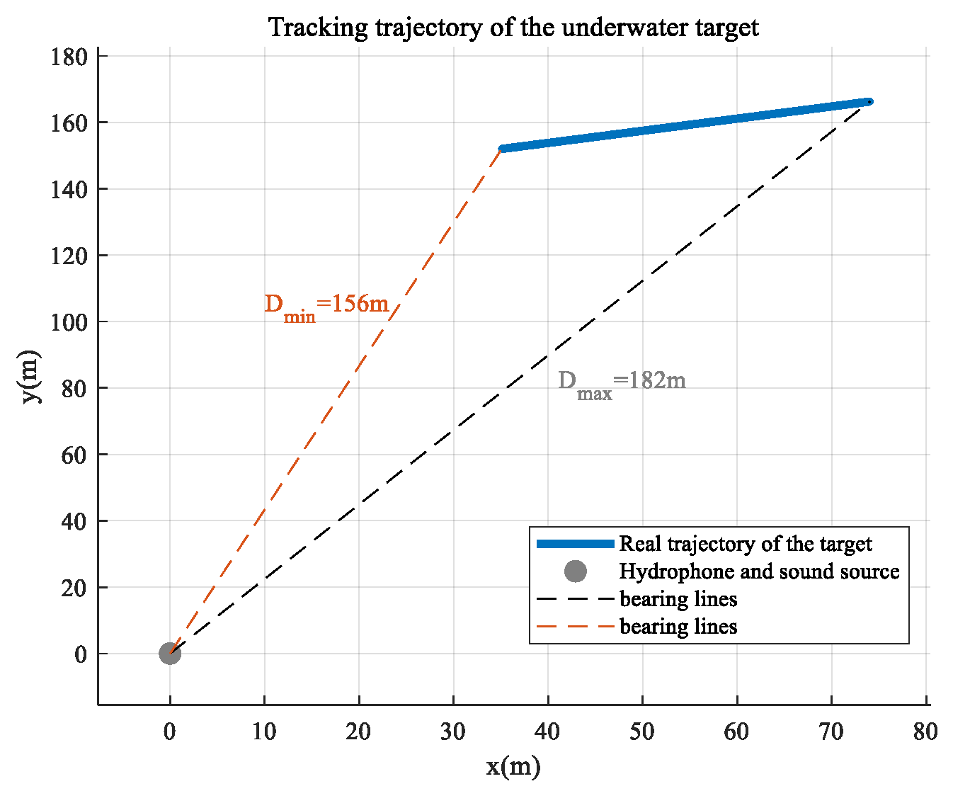
A 48-element horizontal receiver array was employed, which was secured to a support frame and submerged via a rope to 5 m beneath the water surface. The inter-element distance measured 0.05 m, while a 192 kHz rate was used for data acquisition. For the accurate spatial referencing of the target with respect to the sensor array, a Global Positioning System (GPS) was installed on the target. This GPS unit delivered dependable location and temporal data, logging the geographic coordinates for both the acoustic transmitter and the subsea buoy system at one-second intervals. Figure 4 illustrates the calculated path of the target, as well as the locations of the directional acoustic source and the sensor array.

6.2. Data Processing of Experiments and Algorithm Verification

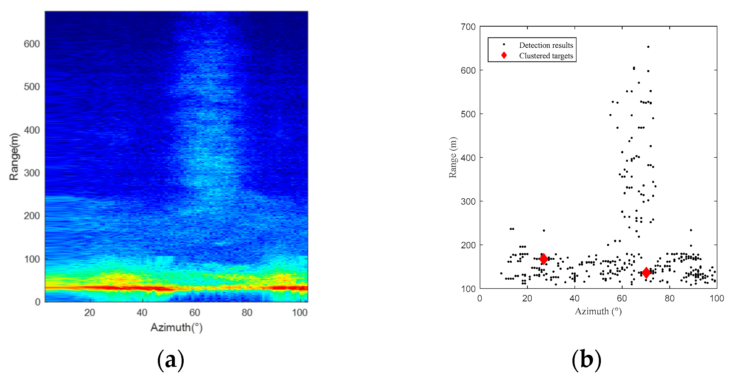
When validating experimental outcomes, the first echoes from active sonar undergo a sequence of conventional processing steps, including matched filtering, beamforming, target detection, and clustering. These techniques improve the signal-to-noise ratio of the echoes and enable the preliminary recognition and differentiation of multiple objects. It is important to emphasize that these steps mainly constitute the essential groundwork for testing the introduced algorithm. Consequently, they are not discussed extensively here. The data fed into the following multi-target tracking method consists of the target returns isolated by the previously described operations. Below, only the displayable images of one frame after each algorithmic processing step are provided, as shown in Figure 5.
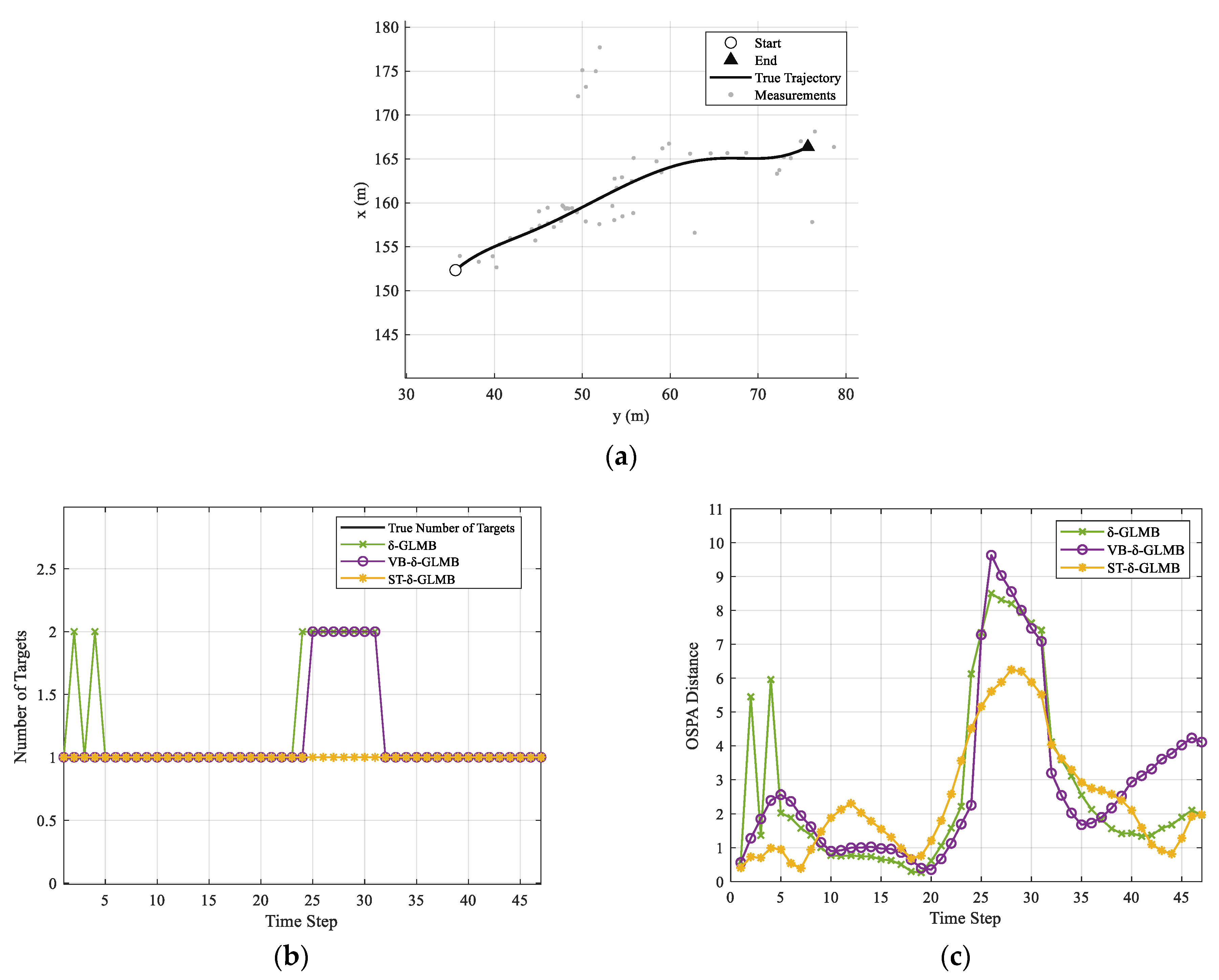
Using the identical procedures outlined previously on every frame yields the data necessary for the multi-target tracking algorithm. A total of 47 valid pings of measurements were obtained for algorithm validation. In the experiment, we employed four multi-target tracking algorithms: CPHD, δ-GLMB, VB-δ-GLMB, and ST-δ-GLMB, using all 47 sets of valid measurement data to validate the proposed algorithm. The GLMB was configured with a fixed noise covariance matrix, while the two adaptive GLMB methods (VB-δ-GLMB and ST-δ-GLMB) were initialized with the same noise covariance matrix. All remaining common variables—including the quantity of newly introduced targets, the likelihood of detection, the chance of survival, and the upper limit on the hypothesis count—were maintained uniformly for every method. It should be noted that the experimental measurements exhibit noticeable non-stationary and non-Gaussian characteristics, especially in the middle portion of the 47-ping sequence (approximately pings 25–30), where the measurement dispersion increases significantly, and several measurements deviate markedly from the main track. As also shown in the measurement plot, these abnormal measurements are mainly concentrated in the spatial region around y = 50∼55 m.
Based on the test data results shown in Figure 6, Figure 6a presents the target’s observational data and its GPS path; a black line indicates the route, while gray points denote the collected readings. It can be observed that non-stationary measurements clearly appear in the y-axis range of 50 m to 55 m. As seen in Figure 6b, in the relatively stable segments (approximately time steps 5–20 and 32–47), all three methods can basically maintain estimates close to the true target number. However, the traditional GLMB exhibits obvious over-estimations around steps 0–5 and 25–30, temporarily judging the target number as two, indicating its insufficient robustness to abrupt non-stationary measurement surges. VB-δ-GLMB significantly alleviates this problem through the online updating of noise statistics, showing only short-lived deviations near the strongest interference (around steps 25–30). ST-GLMB does not show misjudgment in the above periods because the Student’s t-modeling of measurement noise allows it to better adapt to non-stationary measurement noise.
The OSPA distance shown in Figure 6b further quantifies the tracking accuracy. In the steady-state segments, ST-GLMB and VB-δ-GLMB maintain an overall lower OSPA (the curve is close to zero and fluctuates less), outperforming the traditional GLMB. Near the strongest interference/maneuvering (around steps 25–30), all three methods exhibit peaks, but the traditional GLMB has the highest peak and the slowest recovery, VB-δ-GLMB is next, while ST-δ-GLMB has the lowest peak and the fastest recovery. The mechanism behind these differences is as follows: the measurement noise in the test environment exhibits obvious non-stationary characteristics. The traditional GLMB, based on the Gaussian assumption, is easily affected by non-stationary measurement noise, leading to the over-estimation of cardinality and trajectory fragmentation. VB-δ-GLMB improves adaptability to statistical drift through the variational Bayesian online estimation of noise precision. ST-δ-GLMB further employs a heavy-tailed Student’s t measurement model to characterize outliers, combined with label consistency and gating constraints, which significantly reduces false births and target merges induced by non-stationary measurements, thereby achieving a more robust performance in both target number estimation and OSPA. Overall, ST-δ-GLMB demonstrates the strongest robustness against non-stationary noise and strong clutter in real sea-trial environments, effectively reducing the overall position error while ensuring stable target number estimation.

7. Conclusions

During the active sonar tracking of multiple underwater targets, strong reverberation results in measurement disturbances that display pronounced non-stationary and non-Gaussian properties. Multi-target tracking algorithms under Gaussian assumptions will cause significant increases in OSPA distance and target identity label switching in such circumstances. To resolve this problem, the present study introduces a resilient algorithm for tracking multiple underwater targets, named ST-δ-GLMB, which is founded on the Student’s t-framework. This method models the time-varying and non-Gaussian properties of sensor noise via the Student’s t-distribution and employs a variational Bayesian inference to accomplish real-time parameter estimations for the noise. This work introduces analytical derivations and recursive updates utilizing Student’s t-distributed measurement noise, which markedly enhances the multi-target tracking filter’s accuracy. The improvements are validated via the Monte Carlo simulation and verification with real-world lake-trial data, and it is shown that under non-stationary and non-Gaussian measurement conditions, compared with algorithms based on Gaussian assumptions, ST-δ-GLMB can effectively suppress the increase in OSPA and label switching, maintaining the continuity of trajectories and the stability of target number estimation.

Author Contributions

Conceptualization, K.Y. and X.H.; methodology, K.Y. and X.H.; software, K.Y.; validation, K.Y.; writing—original draft preparation, K.Y.; writing—review and editing, X.H. and Y.Y.; supervision, X.H. and Y.Y. All authors have read and agreed to the published version of the manuscript.

Funding

This research was funded by the National Natural Science Foundation of China, Grant No. 62341023.

Data Availability Statement

The data presented in this study are not publicly available due to restrictions.

Conflicts of Interest

Author Kaiqiang Yang was employed by the company Hai Ying Enterprise Group Co., Ltd. The remaining authors declare that the research was conducted in the absence of any commercial or financial relationships that could be construed as a potential conflict of interest.

References

  1. Hou, X.; Qiao, Y.; Zhang, B.; Yang, Y. Robust underwater direction-of-arrival tracking based on variational Bayesian extended Kalman filter. JASA Express Lett. 2023, 3, 014801. [Google Scholar] [CrossRef]
  2. Hou, X.; Chen, Y.; Zhang, B.; Yang, Y. Review of research progress on passive direction-of-arrival tracking technology for underwater targets. Remote Sens. 2024, 16, 4511. [Google Scholar] [CrossRef]
  3. Zhang, B.; Hou, X.; Yang, Y. Robust underwater direction-of-arrival tracking with uncertain environmental disturbances using a uniform circular hydrophone array. J. Acoust. Soc. Am. 2022, 151, 4101. [Google Scholar] [CrossRef] [PubMed]
  4. Yang, Y.X.; Zhou, J.B.; Li, M.Y.; Hou, X.; Yang, L.; Xie, L.; Wang, L.; Shen, H.; Liu, X.; Lei, B.; et al. Underwater acoustics: Current status and future trends. Tech. Acoust. 2025, 44, 309–332. [Google Scholar]
  5. Baisa, N.L.; Wallace, A. Multiple target multiple type filtering in the RFS framework. Digit. Signal Process. 2019, 89, 49–59. [Google Scholar] [CrossRef]
  6. Li, H.L.; Chen, B.X.; Ding, Y.; Zhang, Z.M. Nearest-neighborhood data association algorithm based on information entropy weighting. Syst. Eng. Electron. 2020, 42, 806–812. [Google Scholar]
  7. Chen, J.; Leung, H.; Lo, T.; Litva, J.; Blanchette, M. A modified probabilistic data association filter in a real clutter environment. IEEE Trans. Aerosp. Electron. Syst. 1996, 32, 300–313. [Google Scholar] [CrossRef]
  8. Reid, D.B. An algorithm for tracking multiple targets. IEEE Trans. Autom. Control 1979, 24, 843–854. [Google Scholar] [CrossRef]
  9. Mahler, R.P.S. Multitarget Bayes filtering via first-order multitarget moments. IEEE Trans. Aerosp. Electron. Syst. 2003, 39, 1152–1178. [Google Scholar] [CrossRef]
  10. Wang, Y.; Luo, Z.J.; Wang, Y.Q. An improved GMPHD filtering algorithm and simulation study. Fire Control Radar Technol. 2016, 45, 32–37. [Google Scholar]
  11. Song, L.P.; Yan, C.; Ji, H.B.; Liang, M. PHD filter for tracking multiple extended targets using box particle. Control Decis. 2015, 30, 1759–1765. [Google Scholar]
  12. Mahler, R. PHD filters of higher order in target number. IEEE Trans. Aerosp. Electron. Syst. 2007, 43, 1523–1543. [Google Scholar] [CrossRef]
  13. Zhang, S.C.; Wu, L.B.; Hu, X.M. Sea-surface target tracking algorithm based on GM-CPHD. Mod. Radar 2020, 42, 28–32. [Google Scholar]
  14. Feng, X.X.; Wei, S.; Lu, C.G. Track-before-detect algorithm for multiple targets based on Gaussian particle CPHD filter. Control Decis. 2017, 32, 1991–1996. [Google Scholar]
  15. Vo, B.T.; Vo, B.N. Labeled random finite sets and multi-object conjugate priors. IEEE Trans. Signal Process. 2013, 61, 3460–3475. [Google Scholar] [CrossRef]
  16. Papi, F.; Vo, B.N.; Vo, B.T.; Fantacci, C.; Beard, M. Generalized labeled multi-Bernoulli approximation of multi-object densities. IEEE Trans. Signal Process. 2015, 63, 5487–5497. [Google Scholar] [CrossRef]
  17. Dong, X.; Zhao, J.; Sun, M.; Zhang, X.; Wang, Y. A modified δ-generalized labeled multi-Bernoulli filtering for multi-source DOA tracking with coprime array. IEEE Trans. Wirel. Commun. 2023, 22, 9424–9437. [Google Scholar] [CrossRef]
  18. Cai, H.; Houssineau, J.; Jones, B.A.; Jah, M.; Zhang, J. Possibility generalized labeled multi-Bernoulli filter for multitarget tracking under epistemic uncertainty. IEEE Trans. Aerosp. Electron. Syst. 2023, 59, 1312–1326. [Google Scholar]
  19. Li, C.Y.; Li, Y.; Ji, H.B.; Shi, R.Z. One-step data association GLMB algorithm for extended target tracking. J. Xidian Univ. 2020, 47, 137–143. [Google Scholar]
  20. Shan, J.Y.; Lu, Y.; Ling, H.Y. Robust adaptive multi-target tracking algorithm for airborne passive radar. Syst. Eng. Electron. 2024, 46, 2902–2915. [Google Scholar]
  21. Shim, C.; Vo, B.-T.; Vo, B.-N.; Ong, J.; Moratuwage, D. Linear complexity Gibbs sampling for generalized labeled multi-Bernoulli filtering. IEEE Trans. Signal Process. 2023, 71, 1981–1994. [Google Scholar] [CrossRef]
  22. Vo, B.-T.; Vo, B.-N. A random finite set conjugate prior and application to multi-target tracking. In 2011 7th International Conference on Intelligent Sensors, Sensor Networks and Information Processing; IEEE: New York, NY, USA, 2011; pp. 431–436. [Google Scholar]
  23. Hou, X.; Chen, Y.; Hua, W.; Yang, Y. Robust DOA tracking of an underwater target in non-Gaussian and non-stationary environmental noise. IEEE Trans. Aerosp. Electron. Syst. 2025, 61, 15412–15437. [Google Scholar] [CrossRef]
  24. Yang, J.L.; Ge, H.W. Adaptive probability hypothesis density filter based on variational Bayesian approximation for multi-target tracking. IET Radar Sonar Navig. 2013, 7, 959–967. [Google Scholar] [CrossRef]
  25. Zhang, B.; Hou, X.; Yang, Y.; Zhou, J.; Xu, S. Variational Bayesian cardinalized probability hypothesis density filter for robust underwater multi-target direction-of-arrival tracking with uncertain measurement noise. Front. Phys. 2023, 11, 1142400. [Google Scholar] [CrossRef]
  26. Zhang, B.X.; Yang, Y.X.; Hou, X.H. Robust underwater multi-target bearing tracking under uncertain measurement noise. Acta Acust. 2023, 48, 605–617. [Google Scholar]
  27. Yang, J.; Ge, H. An improved multi-target tracking algorithm based on CBMeMBer filter and variational Bayesian approximation. Signal Process. 2013, 93, 2510–2515. [Google Scholar] [CrossRef]
  28. Qiu, H.; Huang, G.; Gao, J. Variational Bayesian labeled multi-Bernoulli filter with unknown sensor noise statistics. Chin. J. Aeronaut. 2016, 29, 1378–1384. [Google Scholar] [CrossRef]
  29. Yuan, C.; Wang, J.; Xiang, H.; Sun, J. Adaptive δ-GLMB filtering algorithm based on VB approximation. Syst. Eng. Electron. 2017, 39, 237–243. [Google Scholar]
  30. Huang, Y.; Zhang, Y.; Wu, Z.; Chambers, J.A. A novel robust Student’s t-based Kalman filter. IEEE Trans. Aerosp. Electron. Syst. 2017, 53, 1545–1554. [Google Scholar] [CrossRef]
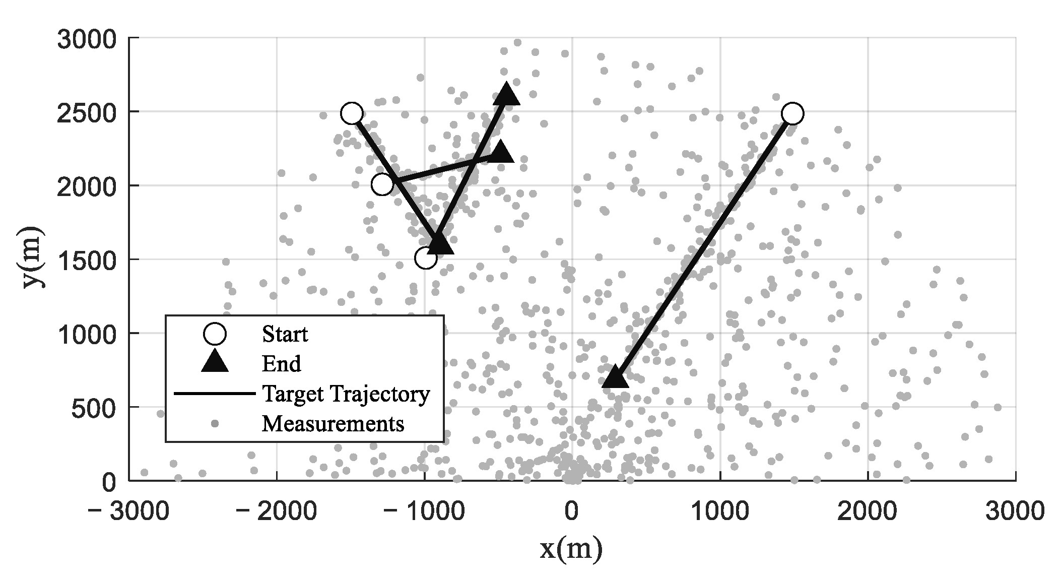
Figure 1. Schematic diagram of target and trajectory measurements.
Remotesensing 18 01332 g001
Figure 2. Experimental results. (a): target number results and (b): OSPA distance results.
Remotesensing 18 01332 g002
Figure 3. Tracking results of a single experiment for different algorithms. (a) results of CPHD; (b) results of δ-GLMB; (c) results of VB-δ-GLMB; and (d) results of ST-δ-GLMB.
Remotesensing 18 01332 g003
Figure 4. True target trajectories and measurements obtained in the field experiment.
Remotesensing 18 01332 g004
Figure 5. Data preprocessing results. (a) matched filtering and broadband beamforming results and (b) target detection and clustering results.
Remotesensing 18 01332 g005
Figure 6. Lake test data results for different algorithms. (a) GPS trajectory and measurements; (b) target number estimation results for different algorithms; and (c) OSPA distance for different algorithms.
Remotesensing 18 01332 g006
Table 1. List of Symbols.
SymbolMeaning
I Label set associated with the current hypothesis
ξ Association-history index of the current hypothesis
θ Measurement-to-track association mapping at the current time step
ω ( I , ξ ) Weight   of   the   hypothesis   indexed   by   ( I , ξ )
p ( ξ ) ( , l ) Single-target posterior density associated with label ℓ under hypothesis ξ
J Surviving label subset in the prediction step
L Birth label subset in the prediction step
λ k Latent variable introduced by the hierarchical Student t representation
q ( x k ) Variational posterior density of the target state
q ( λ k ) Variational posterior density of the latent variable
γ k Shape   parameter   of   the   Gamma   posterior   for   λ k
Table 2. RMSE of target number and average OSPA results.
CPHDδ-GLMBVB-δ-GLMBST-δ-GLMB
RMSE of target number1.370.410.290.13
Average OSPA46.8032.4120.7218.53
Table 3. Average label switch count and average runtime of different methods.
Methodδ-GLMBVB-δ-GLMBST-δ-GLMB
Average Label Switch Count18.712.57.8
Average Runtime (s)16.3418.2719.03
Disclaimer/Publisher’s Note: The statements, opinions and data contained in all publications are solely those of the individual author(s) and contributor(s) and not of MDPI and/or the editor(s). MDPI and/or the editor(s) disclaim responsibility for any injury to people or property resulting from any ideas, methods, instructions or products referred to in the content.