Radiometric Performance Monitoring Method for LuTan-1 Satellites Combining Internal Calibration and Field Calibration

Highlights

What are the main findings?

• A radiometric performance monitoring method combining internal calibration and field calibration is proposed for the Lutan-1 (LT-1) L-band differential interferometric synthetic aperture radar mission.
• The absolute radiometric accuracy of LT-1A is improved from 0.40 dB to 0.25 dB after beam gain correction.

What are the implications of the main findings?

• The method provides a reliable reference for long-term radiometric monitoring of SAR satellites.
• High radiometric accuracy and stability support quantitative InSAR applications of the LT-1 mission.

Abstract

The Lutan-1 (LT-1) mission is the first civilian L-band differential interferometric synthetic aperture radar (SAR) system in China, with interferometry as its primary application. The system comprises two multi-polarimetric satellites, LT-1A and LT-1B. For the purpose of quantitative application from SAR images of Lutan-1 satellites, the relationship between the SAR image intensity and the backscattering coefficient of ground objects should be established by radiometric calibration. Field radiometric calibration provides absolute calibration constants, but it suffers from beam coverage. Internal on-board calibration, by contrast, tracks relative changes in radiometric performance but cannot yield absolute calibration constants. Therefore, we develop a method that combines on-board internal calibration with field radiometric calibration to monitor the radiometric performance of LT-1 satellites and to analyze the variation patterns revealed by both internal and field calibrations. We monitor the amplitude and phase trend of internal calibration, calculate absolute calibration constants from field calibration, and refine and evaluate the absolute calibration constants. We analyzed the internal calibration data and SAR calibration data of the LT-1 satellite from 2023 to 2025. The results show that the TRMs of the LT-1 satellite exhibit a slight decline over time, and the magnitude of the decrease in LT-1B is greater than that of LT-1A. The slight decrease in internal calibration has not yet led to visible changes in the absolute calibration constant for LT-1A, while the absolute calibration constants decrease slightly for LT-1B. After removing the calibration constant outliers and correcting the gain difference among the beams for the LT-1A satellite, absolute radiometric accuracy is improved from 0.40 dB (1σ) to 0.25 dB (1σ). The absolute radiometric accuracy of the LT-1B satellite is 0.38 dB (1σ). It gives a reference for radiometric performance monitoring of the SAR satellite over a long period.

1. Introduction

Synthetic aperture radar (SAR) actively transmits and receives signals and therefore operates in all weather and at all times of day. Many SAR satellites have been launched successfully, including TerraSAR-X and TanDEM-X satellites, Sentinel-1 satellites (including Sentinel-1A, Sentinel-1B, Sentinel-1C and Sentinel-1D), the RADARSAT-2 satellite, ALOS series satellites, Gaofen-3 series satellites, L-band differential interferometric SAR satellites, and HJ-2 05/06 satellites, which support applications in oceanography, surveying and mapping, land resource management, and disaster reduction [1,2,3,4,5]. Radiometric calibration establishes the functional relationship between the SAR image intensity and the backscattering coefficient of ground targets, enabling retrieval of quantitative parameters [6]. Routine radiometric performance assessment of the SAR satellite preserves long-term radiometric consistency and supports scaling applications from regional to global domains [7]. Because satellite radiometric characteristics may change over time and thereby degrade image radiometric accuracy, the long-term radiometric performance needs to be monitored [8,9].

The German Aerospace Center developed a long-term radiometric monitoring system to assess SAR image quality and diagnose occasional failures for the TerraSAR-X and TanDEM-X satellites. The system measured transmit/receiver module (TRM) gain and phase stability using coded calibration pulses, characterized the antenna pattern with distributed targets, and evaluated radiometric stability with long-term deployed corner reflectors [8,9,10,11,12]. Following the successful launch of TanDEM-X in 2009, two years after TerraSAR-X, a second field calibration demonstrated that the radiometric stability of TerraSAR-X was better than 0.2 dB [12]. By 2018, TerraSAR-X had operated for 10 years and TanDEM-X for over 7 years. On-board monitoring showed the TRM amplitude deviation below 0.1 dB and phase deviation below 1°, while field results demonstrated the RCS standard deviation of three corner reflectors (1.5 m leg length) below 0.2 dBsm. The absolute calibration accuracies for the two satellites were 0.34 dB and 0.33 dB, respectively. These values included field calibration errors of 0.16 dB for TerraSAR-X and 0.14 dB for TanDEM-X, a dynamic slant-range error of 0.10 dB, and a maximum atmospheric loss of 0.24 dB due to rainfall [8]. Overall, the long-term radiometric quality of the SAR images remained highly stable. ESA published the annual reports on the performance of the Sentinel-1A/B satellites, which provided a detailed description of TRM variations and radiometric calibrations [13,14,15]. Monitoring of the Sentinel-1B payload between 1 June and 1 August 2016 showed that the average drifts in amplitude and phase were 0.15 dB and 4°, respectively [16]. When the TRM amplitude and phase of the Sentinel-1A/1B satellites fluctuate within a certain range, the radiometric accuracy is not necessarily degraded [13,14,15]. The absolute calibration constants of Sentinel-1A ranged from −0.75 dB to 0.6 dB during the period from November 2015 to July 2017 [17]. The Sentinel-1B satellite expired on 23 December 2021 [13]. Up to 2024, the absolute radiometric accuracy of Sentinel-1A was better than 0.34 dB (1σ), and until its expiration, Sentinel-1B achieved accuracy better than 0.33 dB (1σ), where the following errors were considered: field calibration errors were 0.25 dB (1σ) for Sentinel-1A and 0.24 dB (1σ) for Sentinel-1B; the dynamic slant distance error was 0.067 dB (1σ); and the accuracy of the reference point target was 0.2 dB (1σ) [14,15]. Sentinel-1C and Sentinel-1D were successfully launched on 6 December 2024 (Beijing time) and 5 November 2025 (Beijing time), respectively. Sentinel-1C started its operational phase after five months of commissioning. After compensation, instrument drift remained low—below 0.1 dB in amplitude and only a few degrees in phase. The stability of the absolute calibration constant for Sentinel-1C was ±0.29 dB, with a reference target accuracy of 0.2 dB, a dynamic range error of 0.067 dB, and a long-term stability of the SAR instrument of 0.05 dB, resulting in an absolute radiometric accuracy of 0.36 dB [18]. Sentinel-1D will replace Sentinel-1A in 2026; test results for Sentinel-1D are not yet available.

Lutan-1 (LT-1) is the first civilian L-band differential interferometric SAR satellite constellation in China, with interferometry as its primary application. The constellation comprises two identical satellites, LT-1A and LT-1B, launched on 26 January and 27 February 2022, respectively. Both satellites have operated for over 4 years. The imaging modes of the Lutan-1 satellites are listed in

Table 1. Imaging modes of the LuTan-1 satellites.

Imaging Mode	Resolution/m	Swath Width/km	Swinging Angle/(°)	Beam Code
				Right Side View	Left Side View
Strip Mode 1	3	50	Imaging 20.0–53.0 Interferometry 20.0–46.0 Extension 10.0–60.0	0–18	222–240
Strip Mode 2	12	100	20.0–46.0	19–23	241–245
Strip Mode 3	3	50	20.0–53.0	0–18	222–240
Strip Mode 4	6	30	13.0–21.6	40–53	262–275
Strip Mode 5	24	160	15.7–30.0	24–25	246–247
SCAN Mode	30	400	20.0–49.0	54–61	276–283

[3]. After completing in-orbit testing on 31 May 2023, LT-1 began nationwide routine observations with Strip Mode 1 [19]. Shi et al. assessed the short-term radiometric stability of LT-1A using Amazon rainforest data [7], but long-term radiometric performance monitoring for the LT-1 constellation remains limited. In this paper, we develop a radiometric performance monitoring method for LT-1 satellites that integrates internal calibration and field radiometric calibration. We monitor amplitude and phase changes from the internal calibration, derive absolute calibration constants from the field calibration, and verify and refine those absolute calibration constants, which reduces abnormal absolute calibration constants within beams and minimizes inter-beam gain errors. Since 2023, we have been conducting a radiometric monitoring experiment for LT-1. By jointly analyzing internal calibration and field calibration, we assess and verify changes in the SAR payload’s radiometric performance rapidly and accurately. The approach provides a reference method for long-term monitoring of SAR radiometric performance and reduces abnormal radiometric calibration constants.

This paper is organized as follows: Section 2 presents the calibration site and the experimental data, including internal calibration data and field calibration data. Section 3 introduces the radiometric performance monitoring process and methods for the LT-1 satellites. Section 4 describes the radiometric performance monitoring results for the LT-1 satellites. Then, Section 5 discusses the radiometric performance monitoring results. Finally, Section 6 gives the conclusions.

2. Study Area and Data

We have analyzed 156 orbits of internal calibration data for the LT-1A satellite and 181 orbits for the LT-1B satellite. The corresponding values for each year from 2023 to 2025 for LT-1A are 45, 39, and 72, while for LT-1B, the corresponding values are 65, 32, and 84. All data were collected from July 2023 to October 2025.

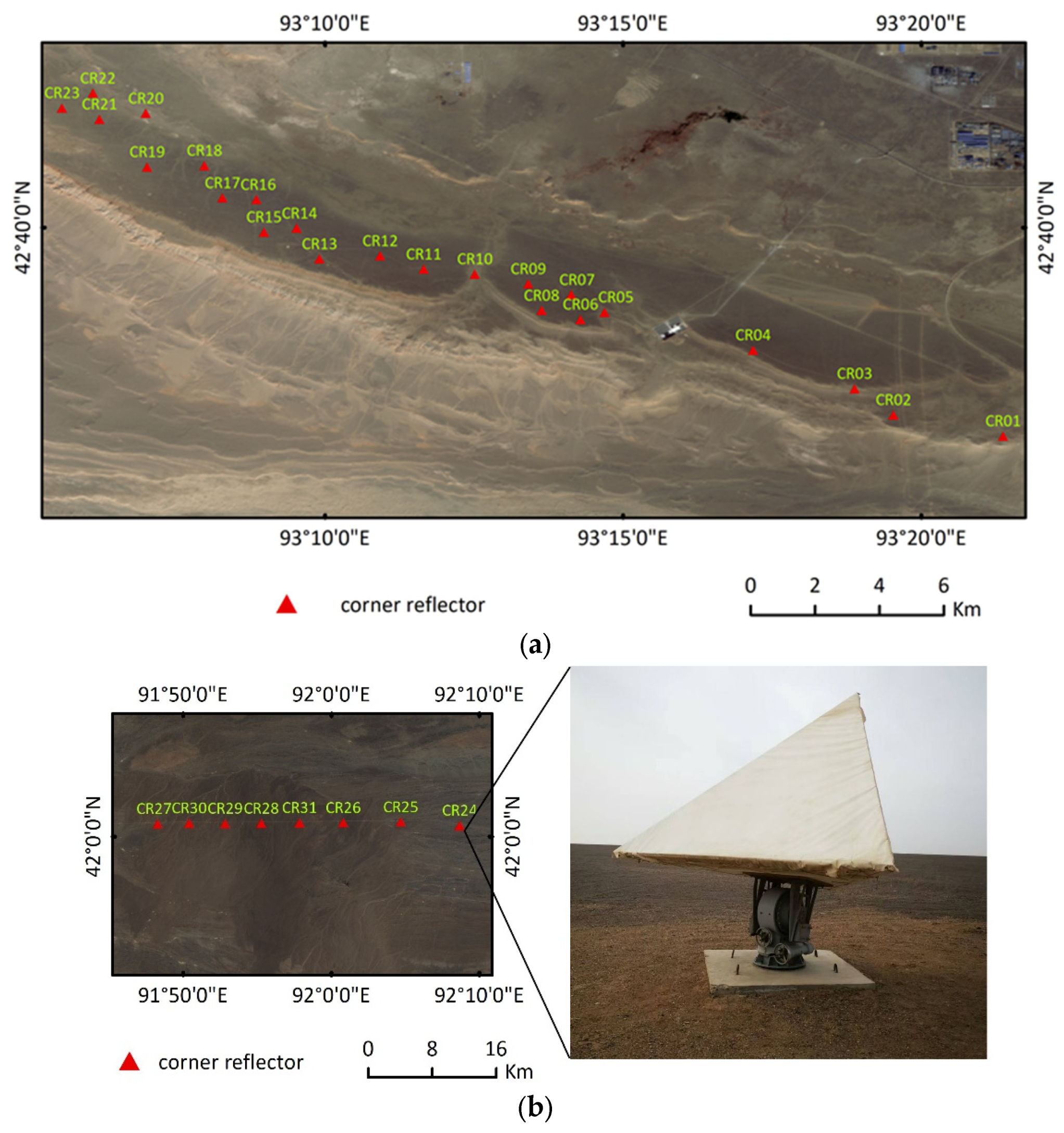
The field calibration site for the LT-1 satellites is located in Hami City, Xinjiang Province. The distribution of corner reflectors is illustrated in Figure 1. The leg length of the corner reflectors is 3 m. There are scale dials to show the azimuth angle and pitch angle on the corner reflectors. During the experiment, we adjusted the azimuth and pitch angles through two wheels on the corner reflectors, and validated the azimuth and pitch angles with the north maker and the level. The measurement accuracy of the north marker is 0.2°, and the measurement accuracy of the level is 0.1°, which ensures that the error of the RCS is less than 0.2 dB.

We have conducted 91 field calibrations campaigns for LT-1A; the corresponding values for each year from 2023 to 2025 are 41, 11, and 39. In contrast, we conducted 84 field calibrations campaigns for LT-1B; the corresponding values for each year from 2023 to 2025 are 36, 10, and 38. Both LT-1A and LT-1B field calibrations occurred from October 2023 to October 2025.

3. A Radiometric Performance Monitoring Method for LT-1 Satellite

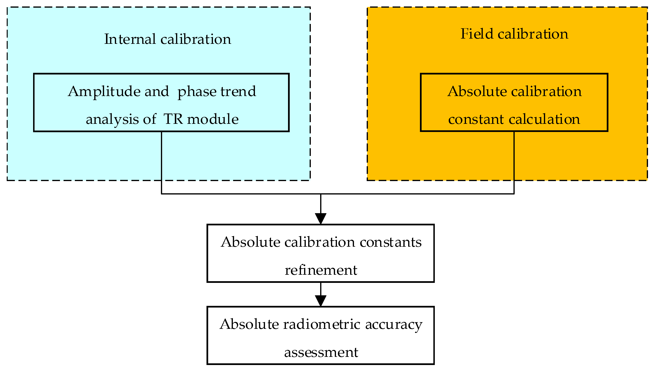
The radiometric quality of SAR images depends on factors ranging from on-board payload to field calibration, so we propose a method to monitor the radiometric performance of the LT-1 satellites. The method comprises three components. First, we monitor trends in the amplitude and phase of the TRM from the on-board internal calibration. Second, we calculate the absolute calibration constants from the field data. Third, we verify the absolute calibration constants. The flowchart is shown in Figure 2.

3.1. On-Board Internal Calibration

The SAR payloads of the LT-1A/B satellites utilize a dual-polarization phased-array system, comprising 352 horizontal (H) and 352 vertical (V) polarization channels. The radiometric stability is monitored by internal calibration loops [20]. LT-1A/B satellites conduct internal calibration before and after imaging, referred to as head calibrations and tail calibrations, respectively. These internal calibration data are transmitted with the echo data, so the calibration status is tracked continuously. We monitor the SAR payload using signals from the TRM calibration loop, employ a matched filter to compress the pulses by using Formula (1), and analyze the amplitude and phase of the transmitting channel and receiving channel for each TRM. The matched filter function is shown as follows [21]:

$$H(f)=exp(j\pi f^2/K)$$

(1)

where $f$ represents the frequency in the range direction, $K$ represents the modulation frequency of the linear frequency modulation signal.

LT-1 satellites are equipped with two channels in the azimuth direction in Strip Mode 1. We can compute the amplitude and phase imbalance of the two channels after pulse compression.

3.2. Field Calibration

Absolute calibration constants for the Sentinel-1A/1B satellites and the ICEYE series satellites incorporated the main lobe energy ratio of point targets [22,23], so we analyzed the influence of that factor and calculated the absolute calibration constant as follows [24].

$$K_{\mathrm{dB}}=10{\log }_{10}{P}_{\mathrm{P}}+10{\log }_{10}S-10{\log }_{10}{\sigma }_{\mathrm{P}}-10{\log }_{10}{C}_{\mathrm{F}}$$

(2)

where $K_{\mathrm{dB}}$ represents decibel of the absolute calibration constant, $P_{\mathrm{P}}$ denotes the point energy excluding the background clutter, $S$ represents the pixel area of the ground range plane, ${\sigma }_{\mathrm{P}}$ represents the RCS of the corner reflector, and $C_{\mathrm{F}}$ represents the main lobe energy ratio of the point target.

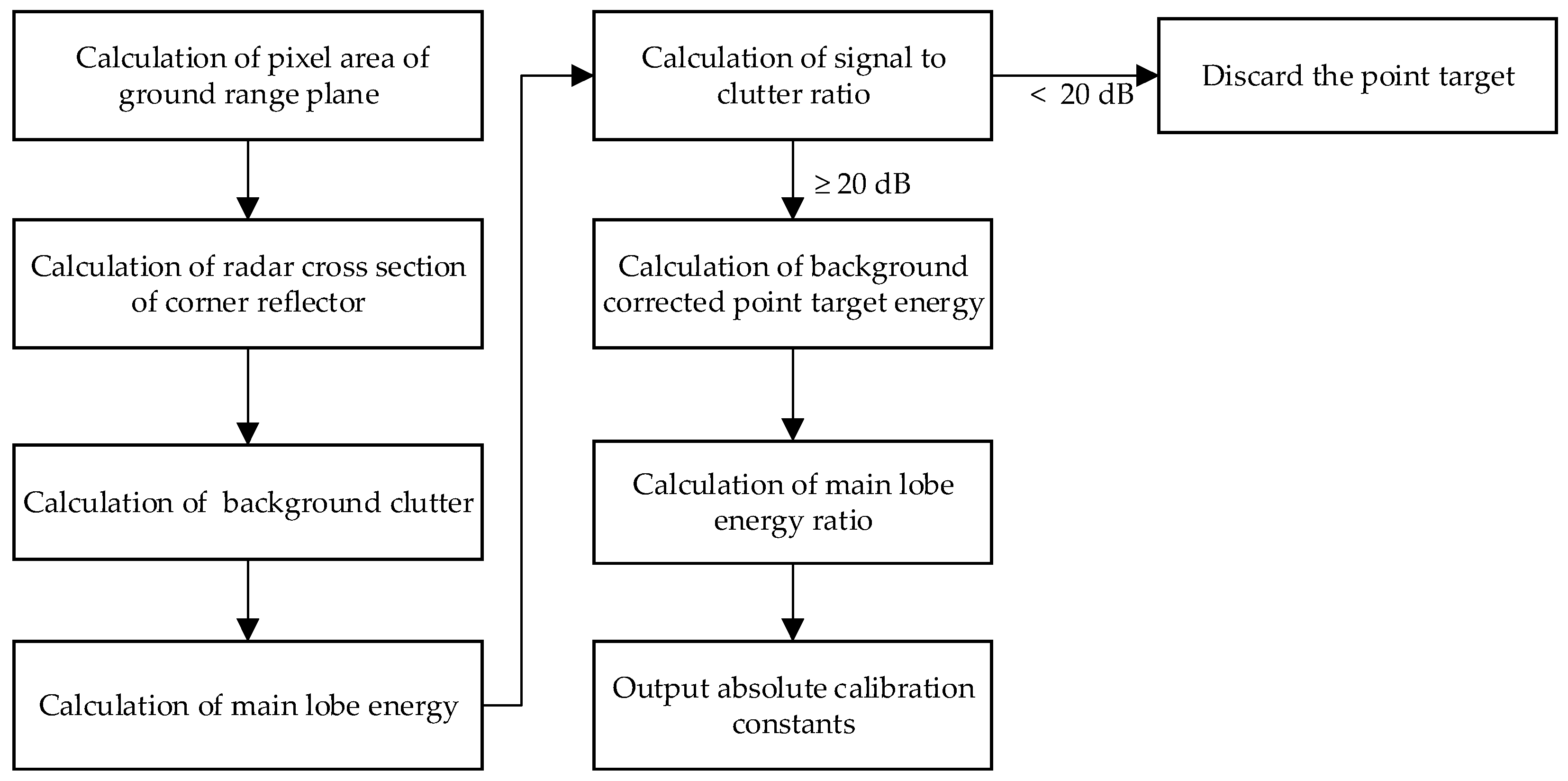
The absolute calibration constant depends on the point target energy, the RCS of the corner reflector, the pixel area of the ground range plane, and the main lobe energy ratio of the point target [22,23]. The procedure of extracting the absolute calibration constant by the integral method is shown in Figure 3.

Step 1: We calculate the pixel area on the ground range plane by using the following Formula [6,22,23,24,25]:

$$S={\delta }_{\mathrm{a}}{\delta }_{\mathrm{r}}/\sin \theta$$

(3)

where $S$ indicates the pixel area of the ground range plane; ${\delta }_{\mathrm{a}}$ and ${\delta }_{\mathrm{r}}$ represent the sampling intervals in the azimuth and slant-range directions, respectively. Additionally, $\theta$ represents the local incidence angle.

Step 2: We calculate the RCS of the trihedral corner reflector by the following Formula [26]:

$${\sigma }_{\mathrm{P}}={\displaystyle \frac{4\pi l^4}{3{\lambda }^2}}$$

(4)

where ${\sigma }_{\mathrm{P}}$ denotes the RCS of the corner reflector, $l$ represents the leg length of the corner reflector, and $\lambda$ represents the wavelength of the SAR payload. The RCS of the CRs is 37.77 dBsm, which can be computed by Formula (4), with the L-band wavelength of 0.2381 m and the leg length of 3 m.

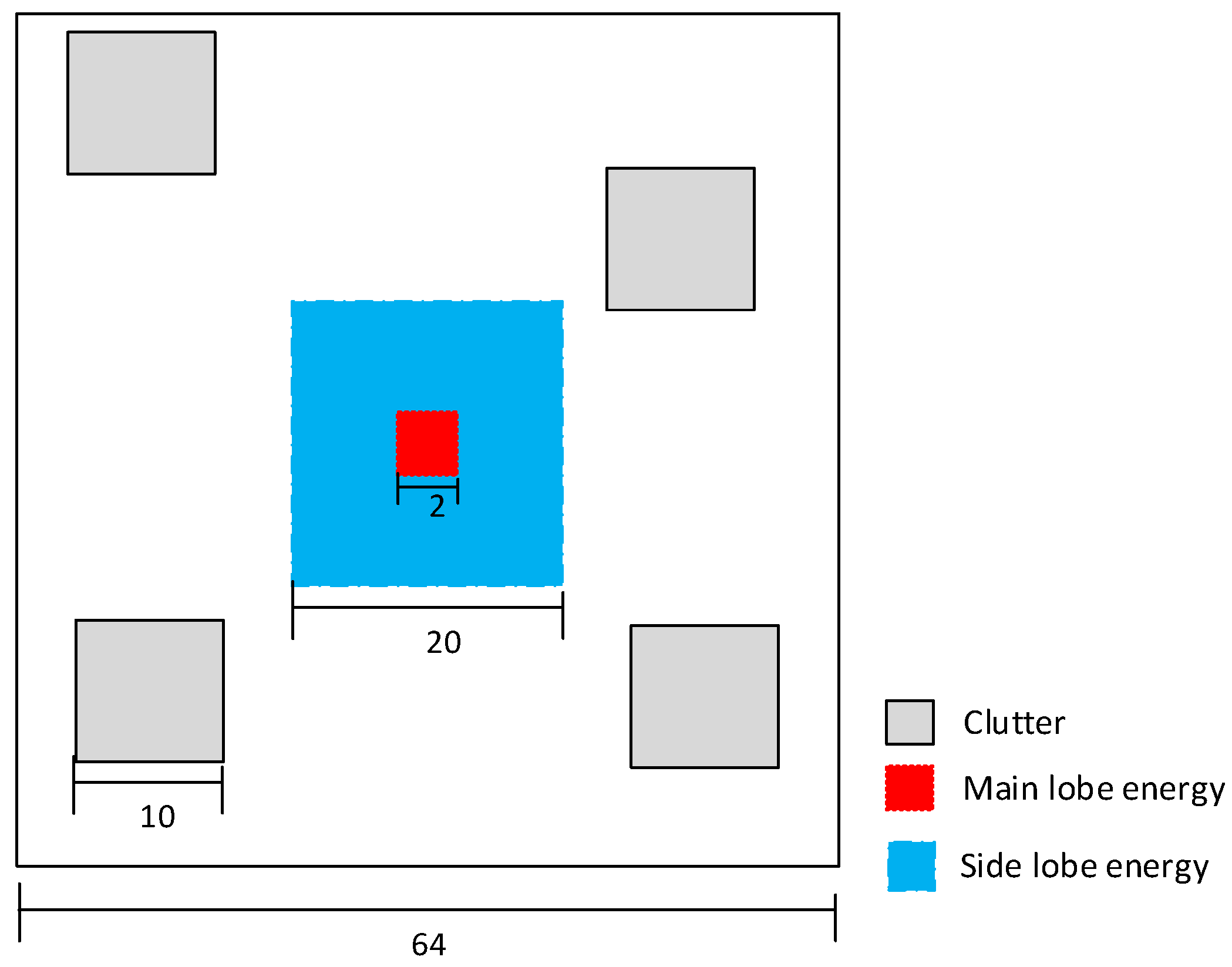
Step 3: We select a data block of 64-by-64 cells centered on the point target and interpolate the block to estimate the energy of the point target. We select 32 as the interpolation multiplier, and the size of the data block is 2048. We reselect a data block of 64-by-64 cells from the interpolated data block and determine areas with a relatively low backscattering coefficient as the background clutter by visual observation, as shown in Figure 4 [6,22,23,24,25]. The window size of the background clutter is set manually, typically 10 × 10 (gray area in Figure 4).

$$P_{\mathrm{clutter}}={\displaystyle \frac{N_{\mathrm{A}}}{N_{\mathrm{B}}}}{\displaystyle \sum _{i\in \mathrm{B}}^{N_{\mathrm{B}}}D{N}^2}$$

(5)

where $P_{\mathrm{clutter}}$ denotes the energy of background clutter, $DN$ denotes the intensity of the background region, $N_{\mathrm{A}}$ denotes the number of pixels within the main lobe energy integration region, $N_{\mathrm{B}}$ denotes the number of pixels corresponding to the background region, and $i$ represents the pixel number.

Step 4: The main lobe energy, indicated by the red area in Figure 4, centers on the point target and spans a two-by-two resolution cell. We compute the main lobe energy by the following Formula [6,22,23,24,25]:

$$P_{\mathrm{main}}={\displaystyle \sum _{i\in \mathrm{A}}^{N_{\mathrm{A}}}D{N}^2}$$

(6)

where $P_{\mathrm{main}}$ denotes the main lobe energy of the point target, which includes the background clutter energy. Additionally, $DN$ denotes the pixel amplitude of the point target; $N_{\mathrm{A}}$ is the same as Equation (5).

Step 5: We subtract the background energy from the point target energy using the following Formula [6,22,23,24,25].

$$P_{\mathrm{P}}=P_{\mathrm{main}}-P_{\mathrm{clutter}}$$

(7)

where $P_{\mathrm{P}}$ represents the background clutter-corrected energy of point target. $P_{\mathrm{clutter}}$ and $P_{\mathrm{main}}$ are the same as in Equations (5) and (6), respectively.

Step 6: Ground clutter significantly reduces the accuracy of SAR radiometric calibration. Therefore, we screen point targets using the signal-to-clutter ratio (SCR) threshold of 20 dB when calculating the absolute calibration constant [6,22,23,24,25]. The SCR is defined by the following equation.

$$SCR=10{\log }_{10}{\displaystyle \frac{P_{\mathrm{P}}}{P_{\mathrm{clutter}}}}$$

(8)

$P_{\mathrm{clutter}}$ and $P_{\mathrm{P}}$ are the same as in Equations (5) and (7), respectively.

Step 7: We select twenty-by-twenty resolution cells centered on the point target as the side lobe energy (blue area in Figure 4), excluding the main lobe of the point target [22,23]. The main lobe energy ratio is defined by the following equation:

$$C_{\mathrm{F}}={\displaystyle \frac{P_{\mathrm{main}}}{P_{\mathrm{sidelobe}}+P_{\mathrm{main}}}}$$

(9)

where $C_{\mathrm{F}}$ denotes the main lobe energy ratio of the point target. $P_{\mathrm{sidelobe}}$ represents the side lobe energy of the point target.

Step 8: We calculate the absolute calibration constant for a single point target using Formula (1), sequentially compute the absolute calibration constants for all point targets that meet the specified criteria, and average these values to obtain the overall absolute calibration constant.

3.3. Calibration Constant Refinement and Accuracy Evaluation

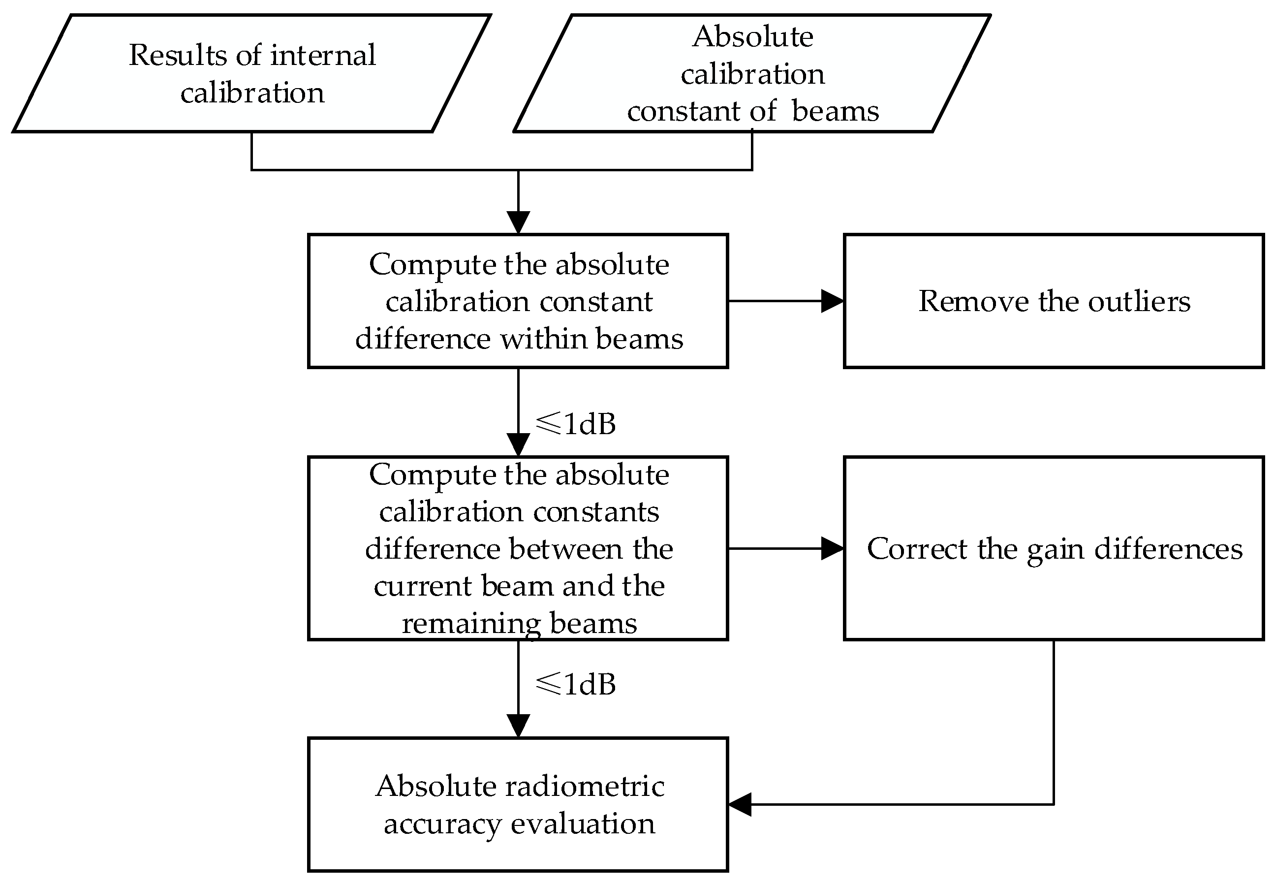
We corrected for transmitting and receiving antenna pattern gains, range and azimuth processing gains, receiver gain control, and range attenuation when generating SAR standard products. However, absolute calibration constants were not uniform. The errors primarily originate from three sources: instrument-related errors, processing-induced errors, and field calibration errors. Instrument-related errors include differences in the peak power among different beams, temporal variations in the antenna patterns, and receiver gain control settings errors. Processing-induced errors include slant-range errors, azimuth and range processing gains, and gains introduced by azimuth and range windowing. Field calibration errors include atmospheric-related errors, RCS errors of calibration equipment, and errors caused by background clutter [8,9,13,14,15]. Amazon rainforest data were used to validate gain differences in the different beams in the early stage. Assuming the normalized backscatter coefficient was consistent among different beams, we computed the gain differences using the backscatter coefficients inverted for each beam. While the normalized backscatter coefficient of the Amazon tropical rainforest varies within approximately 2 dB [27], the absolute calibration constants still fluctuate within a limited range. Therefore, before evaluating absolute calibration constants, we should remove anomalous values within beams and correct inter-beam gain differences. Field calibration cannot obtain repeated measurements at the same beam frequently, or guarantee coverage across different beams. Long-term changes in absolute calibration constants originate from changes in the SAR payload. Therefore, the stability of on-board internal calibration is employed as the criterion: when the internal calibration of the satellite decreased slowly, the absolute calibration constants obtained from the field calibration had no obvious change. This criterion allows us to use multiple field calibration results to identify outliers within beams and to assess gain differences among different beams. Figure 5 illustrates the process of absolute calibration constant refinement and absolute radiometric accuracy evaluation.

Step 1: We determine the outliers of the absolute calibration constant within beams based on the following equation:

$$\Delta K_1=\left|K_i-{\overline{K}}_1\right|$$

(10)

where $\Delta K_1$ denotes the difference in the absolute calibration constant within beams, $K_i$ denotes the absolute calibration constant of the i-th observation, ${\overline{K}}_1$ indicates the averaged absolute calibration constant within beams, and $i$ serves as the observation index. Based on long-term observations, the absolute calibration constant of the Gaofen-3 satellite varies within approximately ±1 dB [28], so the constraint is set to 1 dB. To reduce random error while also considering efficiency, the number of observations is required to be at least five. If $\Delta K_1$ exceeds 1 dB, we remove the absolute calibration constant as an outlier.

Step 2: We use the following equation to judge the gain difference error:

$$\Delta K_2=\left|K_m-{\overline{K}}_2\right|$$

(11)

where $\Delta K_2$ denotes the absolute calibration constant difference between the current beam and the remaining beams, $K_m$ denotes the absolute calibration constant of the m-th beam, ${\overline{K}}_2$ indicates the averaged absolute calibration constant of the remaining beams, and $m$ serves as the beam index. If $\Delta K_2$ exceeds 1 dB, the gain difference error of this beam exceeds the limit. The gain difference for this beam is corrected by $\Delta K_2$.

Step 3: After unifying the absolute calibration constants, we use the standard deviation of the absolute calibration constants to evaluate the absolute radiometric accuracy, as illustrated in Equation (12).

$$\sigma =\sqrt{{\displaystyle \frac{{\displaystyle \sum _{i=1}^N{\left(K_i-\overline{K}\right)}^2}}{N}}}$$

(12)

where $\sigma$ denotes the absolute radiation accuracy, $K_i$ denotes the absolute calibration constant of the i-th observation, $i$ serves as the serial number for the absolute calibration constant, $\overline{K}$ indicates the average value of these constants, and $N$ represents the total number of absolute calibration constants.

4. Experiments and Analyses

4.1. Results and Analysis of Internal Calibration

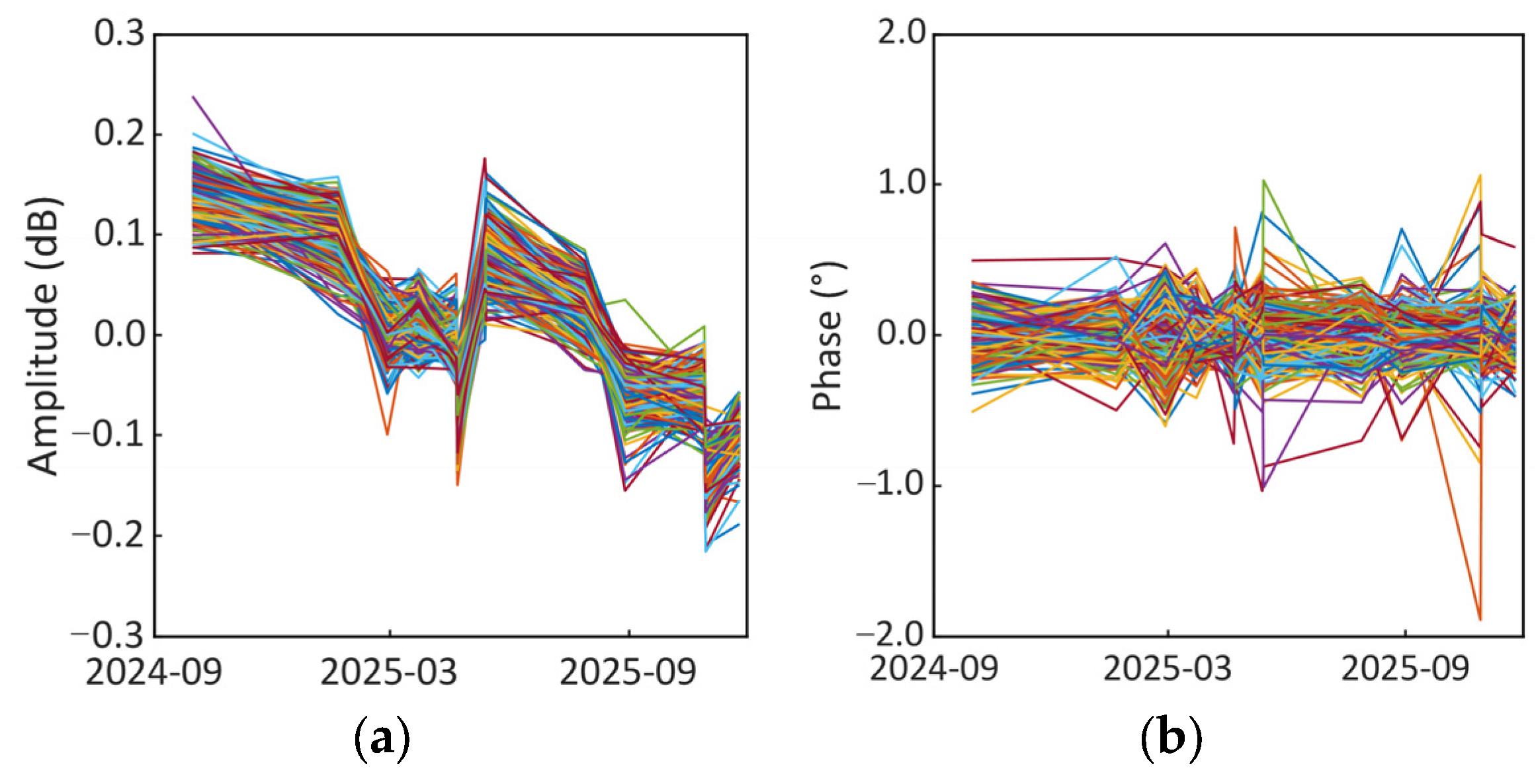
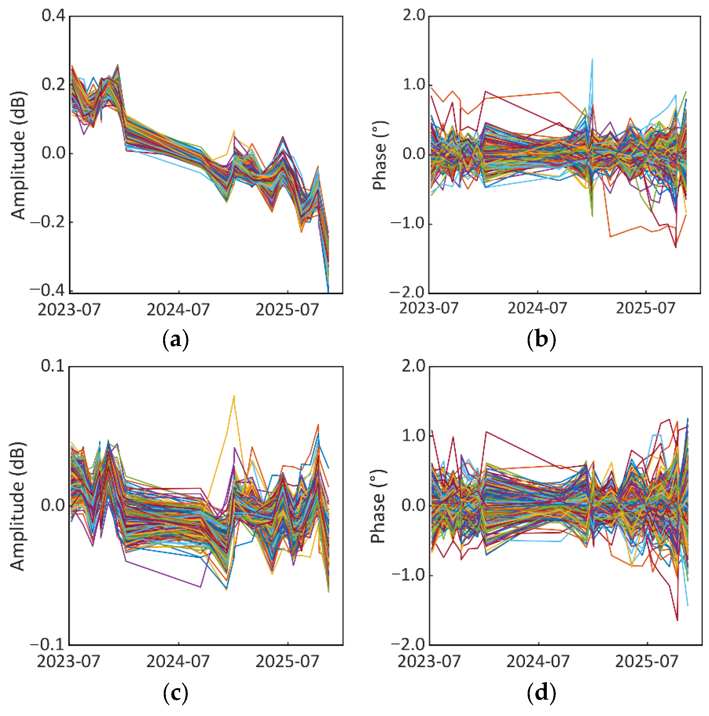
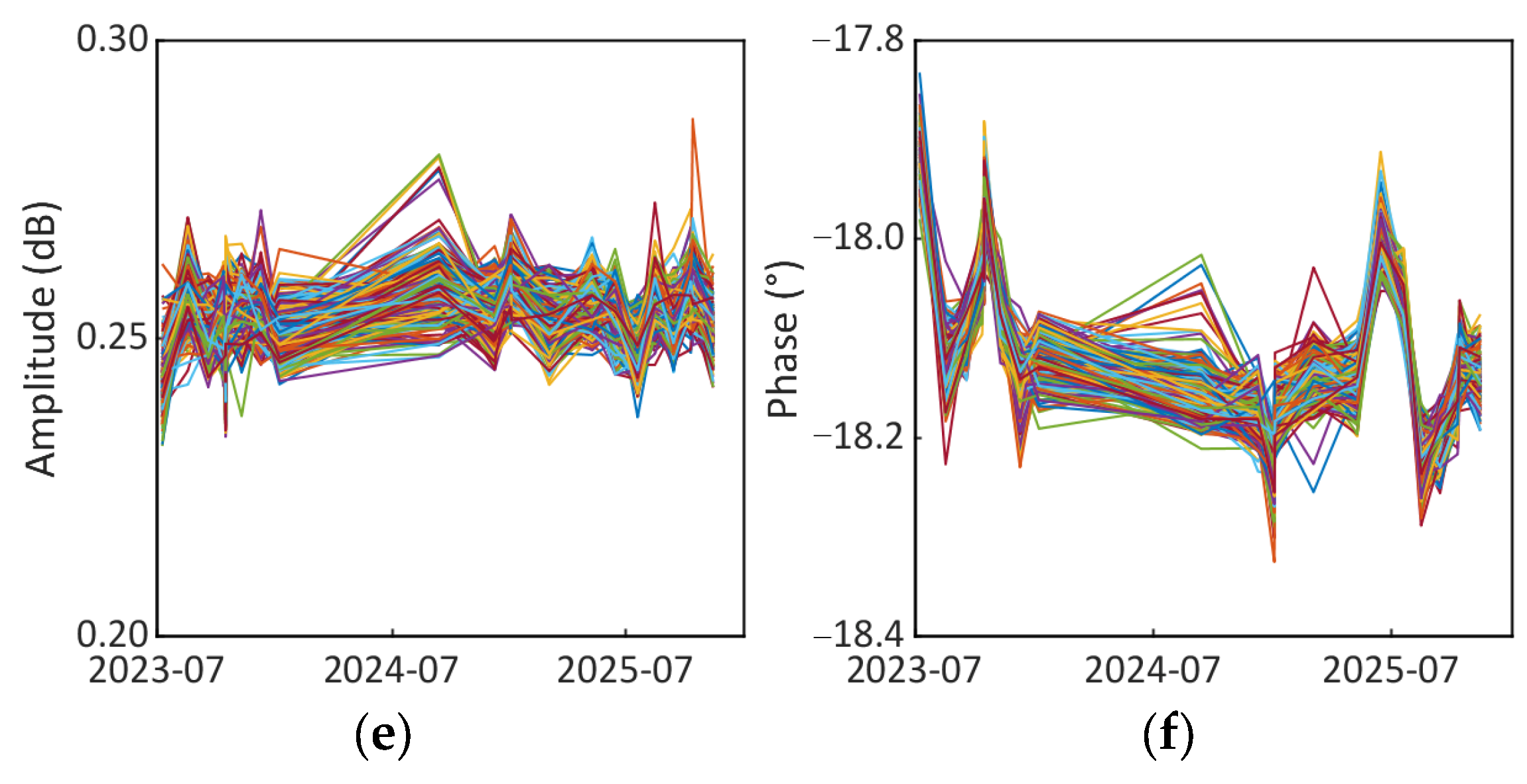
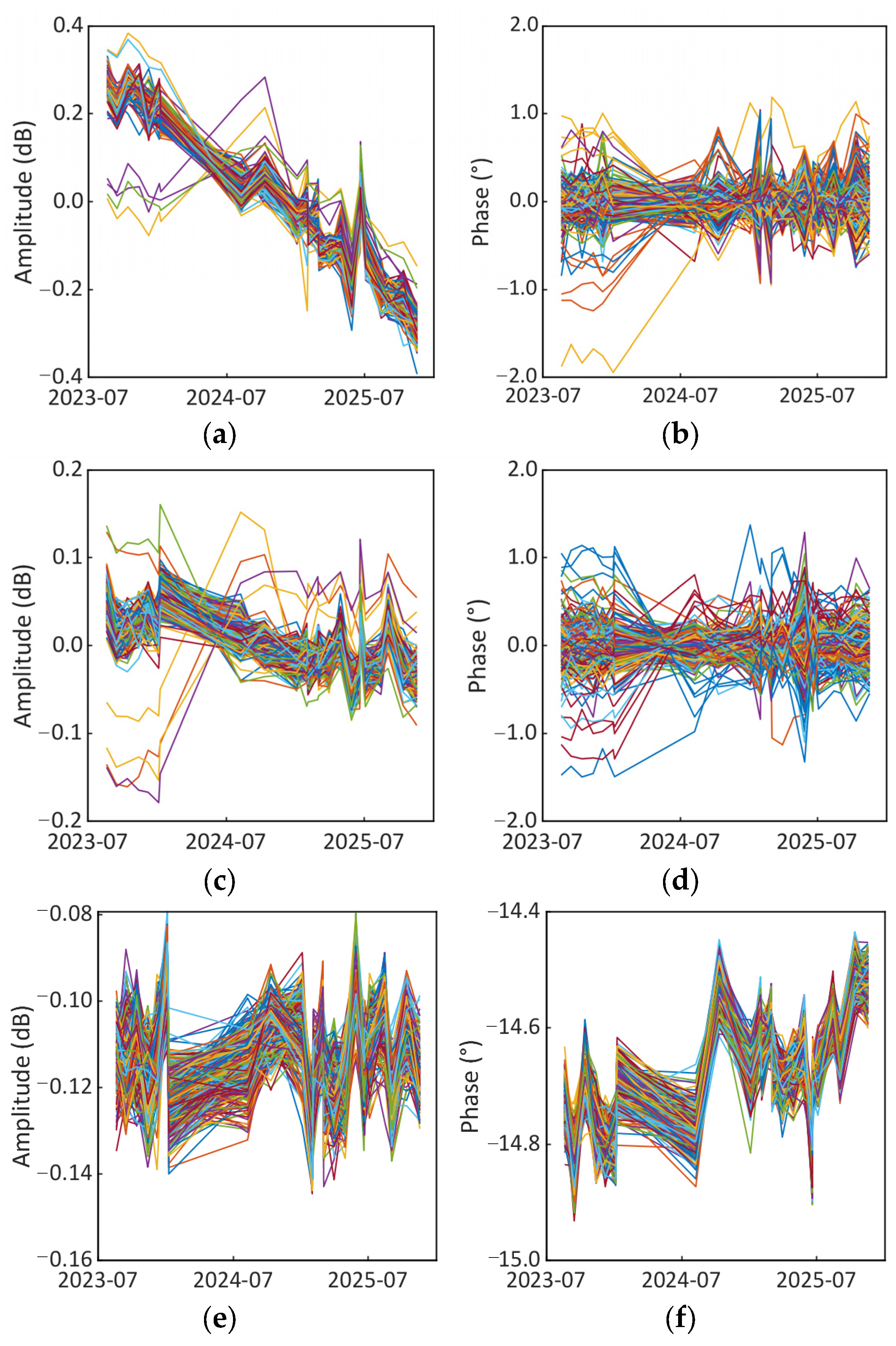
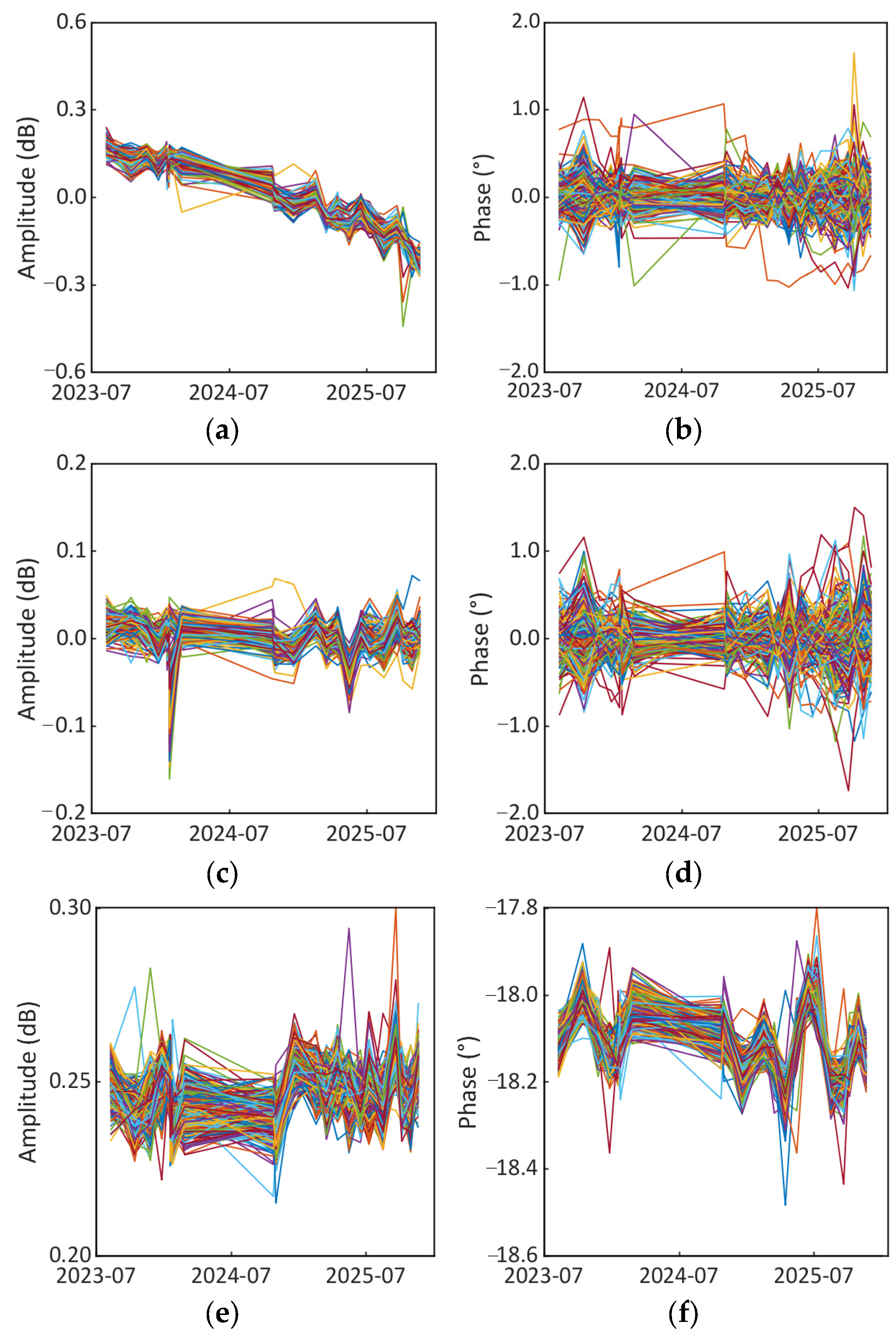
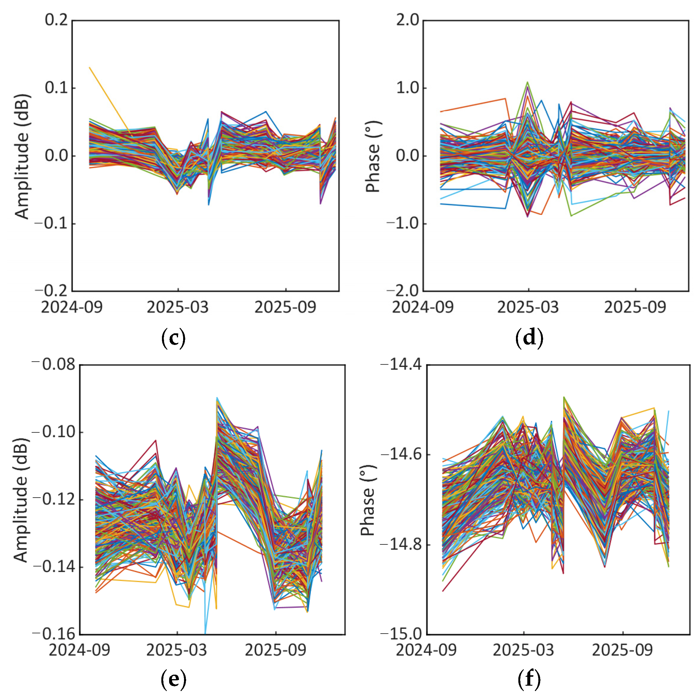
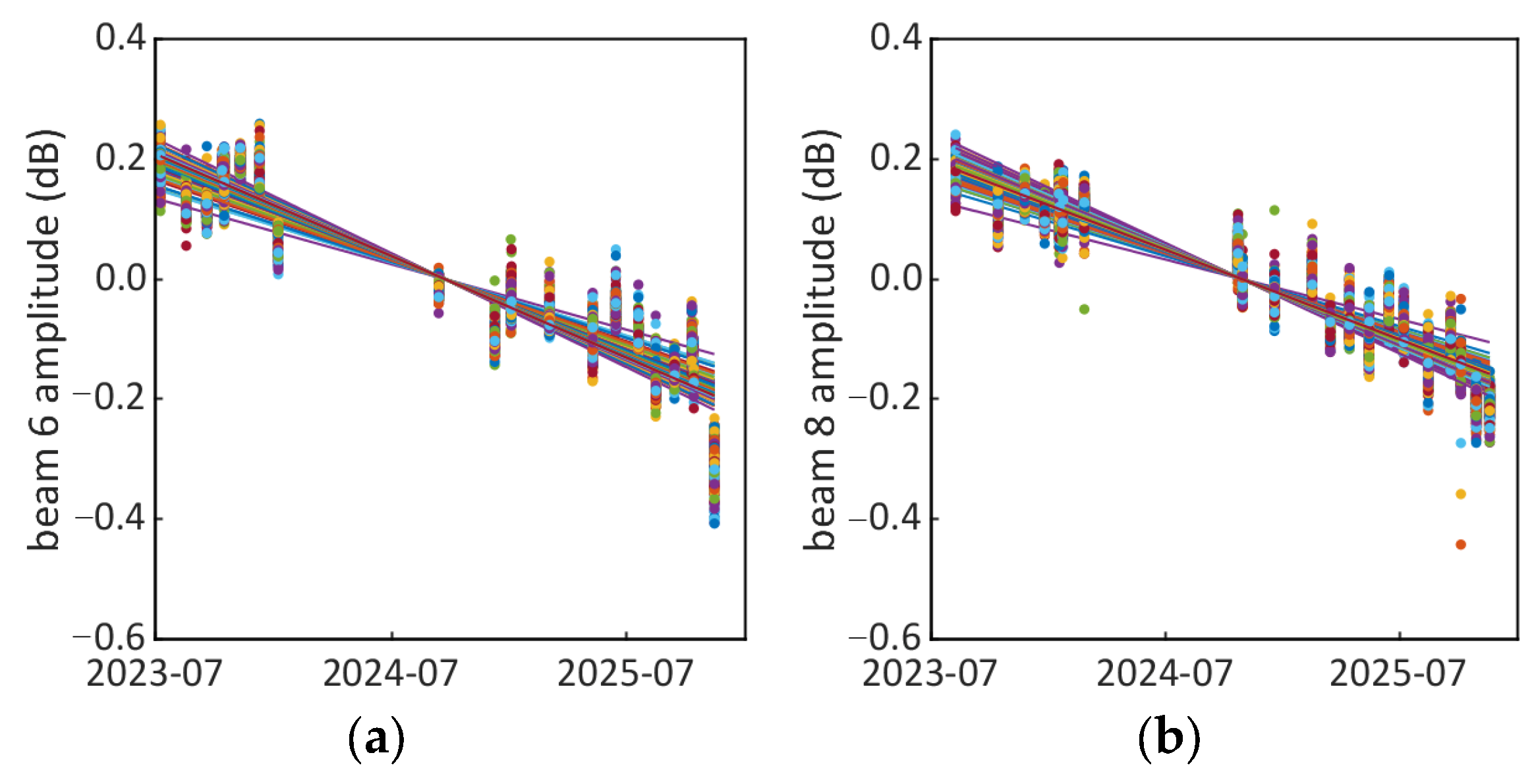
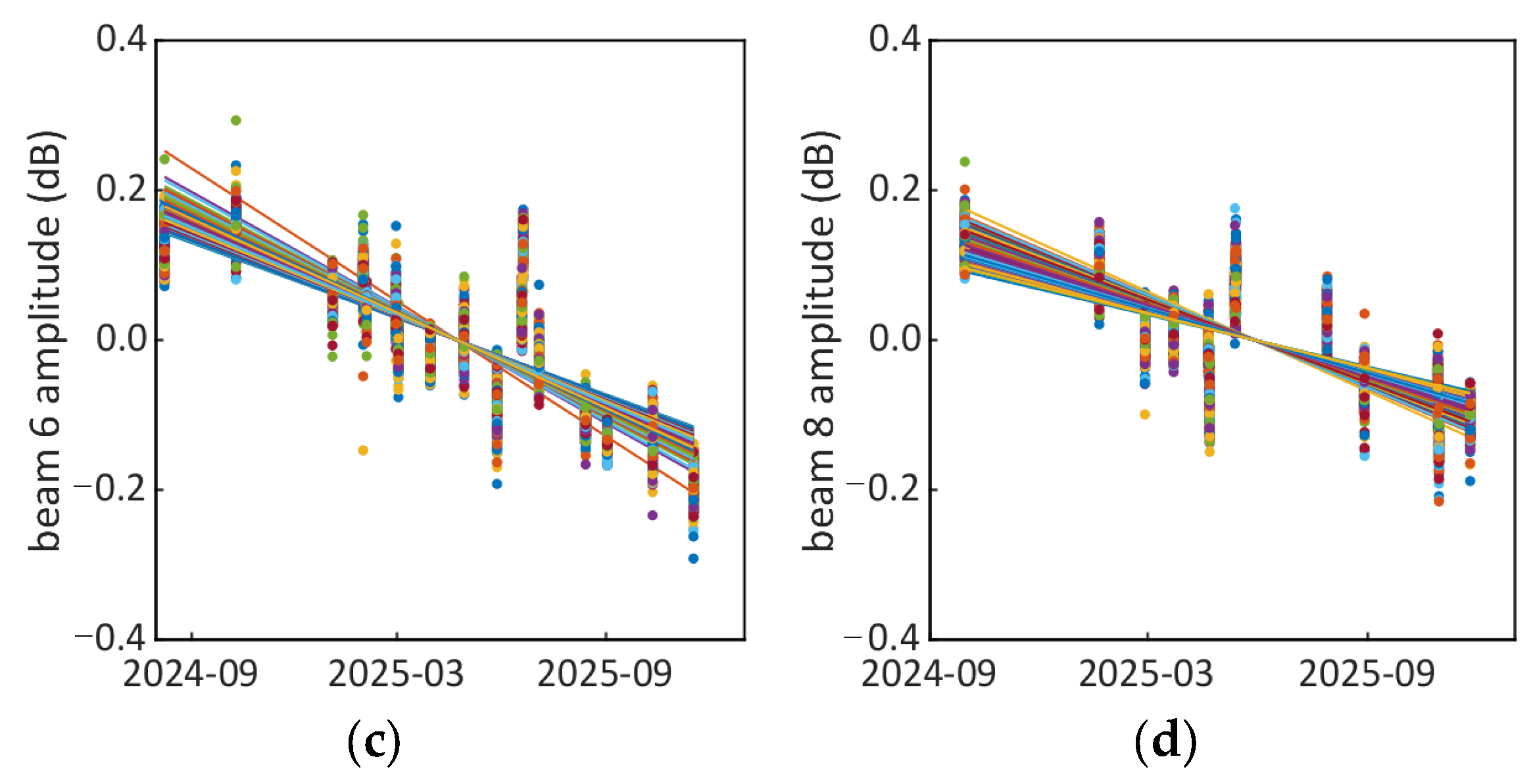
We used the internal calibration data from Strip Mode 1 of the LT-1 satellite to monitor 352 H-polarization transmitting and receiving channels. Most TRM channels operate normally, while the performance of several channels degrades. The amplitude and phase characteristics of SAR satellites at different beams are different. To maintain long-term continuous monitoring, it is necessary to select beams that are frequently used and kept in long-term use. Therefore, we select beams 6 and 8 to illustrate the characteristics of normal TRM channels for long-term observation and further explanation. Figure 6, Figure 7, Figure 8 and Figure 9 displayed these trends, with different colored curves representing different channels. From 2023 to 2025, for the transmitting channels and receiving channels of the LT-1A satellite at beam 6, amplitude standard deviations are better than 0.17 dB and 0.04 dB, respectively, and phase standard deviations are better than 0.93° and 0.76°, respectively. For the transmitting channels and receiving channels of the LT-1B satellite at beam 6, amplitude standard deviations are better than 0.23 dB and 0.11 dB, and phase standard deviations are better than 1.16° and 1.02°. For the transmitting channels and receiving channels of the LT-1A satellite at beam 8, amplitude standard deviations are better than 0.16 dB and 0.04 dB, and phase standard deviations are better than 0.87° and 0.81°. For the transmitting channels and receiving channels of the LT-1B satellite at beam 8, amplitude standard deviations are better than 0.12 dB and 0.04 dB, and phase standard deviations are better than 0.63° and 0.67°. The results indicate a certain reduction in the transmitting channels of the LT-1 satellites, with LT-1B exhibiting a larger reduction than LT-1A. In contrast, the receiving channel remains stable; however, long-term performance requires further verification. For the LT-1A satellite, the amplitude difference in beam 6 between channel 1 and channel 2 is 0.26 dB, with a phase difference of −18.09°. For beam 8, the amplitude difference is 0.25 dB, with a phase difference of −18.09°. For the LT-1B satellite, the amplitude difference in beam 6 is −0.11 dB, with a phase difference of −14.65°. For beam 8, the amplitude difference is −0.12 dB, with a phase difference of −14.60°. The amplitude and phase relationships between channel 1 and channel 2 on both satellites have remained stable over the long term.

The transmitting channels exhibit a declining trend, so we computed the rates of change. Figure 10 shows the decreases in all the TRMs. For the LT-1A satellite, the annual mean decrease in beam 6 from 2023 to 2025 is between 0.11 and 0.19 dB, while beam 8 decreases by 0.10–0.18 dB. For the LT-1B satellite, the TR amplitude trends between 2023 and 2024 are inconsistent; therefore, we consider the period 2024–2025. In that interval, the annual mean decrease in beam 6 is between 0.20 and 0.36 dB, and beam 8 decreases by 0.14–0.26 dB. For the LT-1A satellite, the transmitting channels decreased by approximately 0.4 dB from 2023 to 2025, and for the LT-1B satellite, the transmit channels decreased by approximately 0.6 dB over the same period. The magnitude of the decrease in LT-1B was slightly greater than that of LT-1A.

4.2. Results and Analysis of Absolute Radiometric Calibration

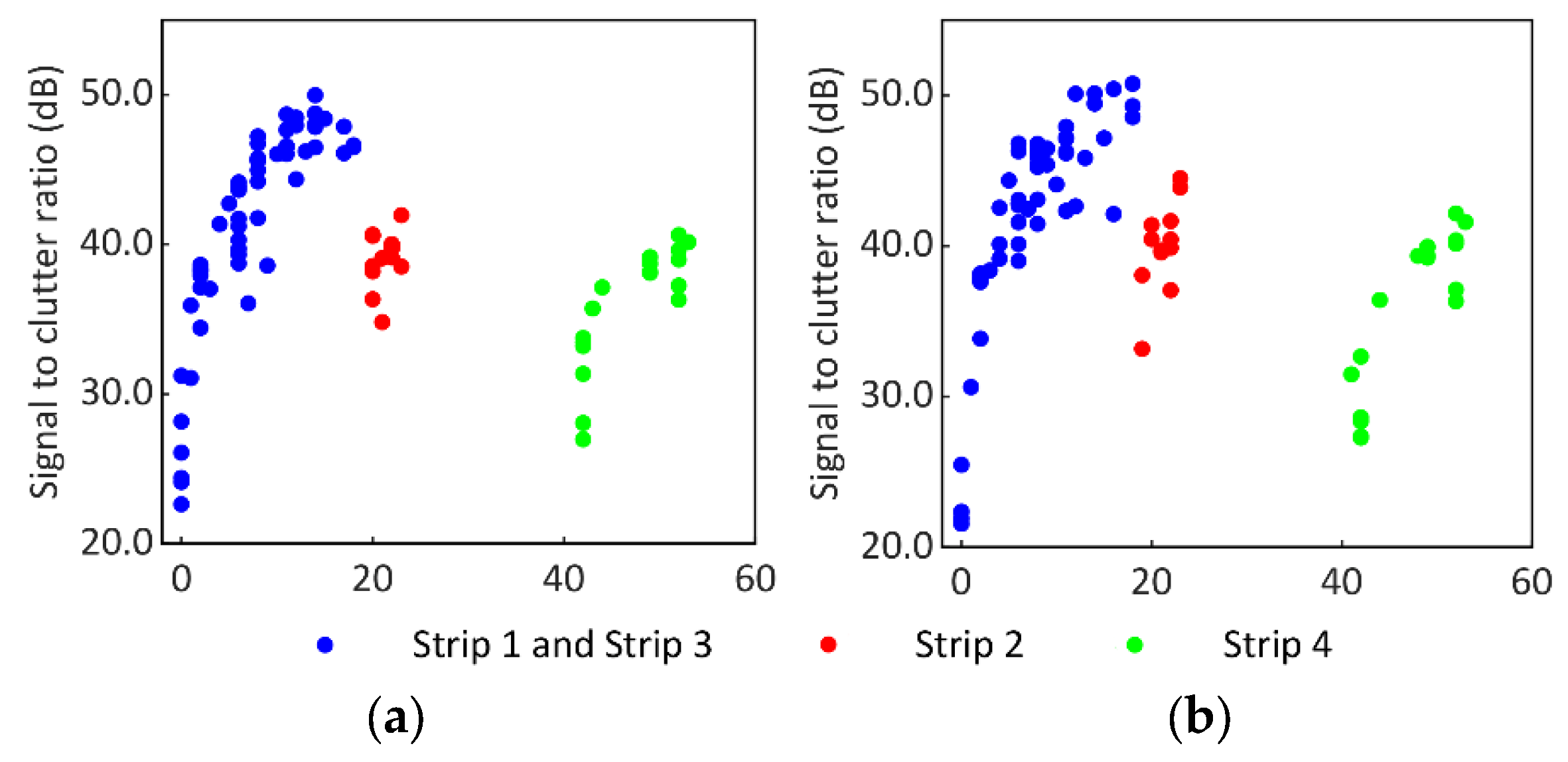
The signal-to-clutter ratios (SCRs) of all point targets exceed 20 dB, as shown in Figure 11. However, beams 0 and 2 exhibit lower SCRs than the other beams. Specifically, beam 0 in Strip Mode 1 typically remains below 30 dB, considerably lower than the SCRs of the remaining beams. Beam 2 mostly falls below 35 dB and therefore shows a clear deficit relative to the others. Two factors explain these deficits. First, both beam 0 and beam 2 of Strip Mode 1 correspond to extended beams. Beam 0 has a central incidence angle of approximately 11.8°, while beam 2 has a central incidence angle of approximately 19.2°. At lower incidence angles, the clutter backscattering coefficient increases and thus reduces the SCR. Second, because the slant-range resolution is designed to be consistent among beams, converting it to ground range yields lower resolution at small incidence angles than at larger ones; this effect can decrease the SCR by up to about 7 dB.

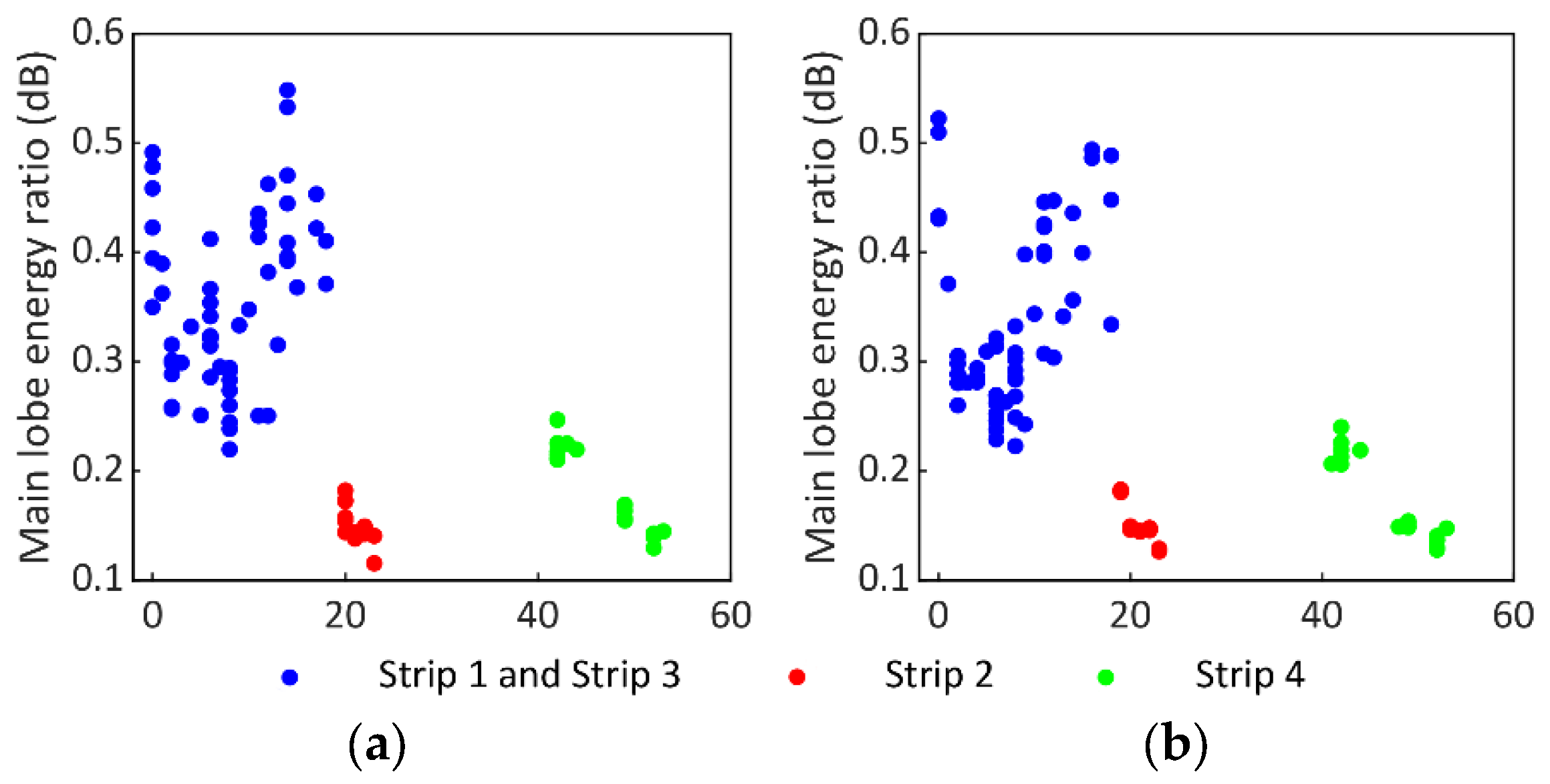
The main lobe energy ratios of point targets in Strip Mode 2 and Strip Mode 4 are less than 0.2 dB, lower than that in Strip Mode 1, as shown in Figure 12. Strip Mode 1 uses an azimuth multi-channel reconstruction method [29], which improves resolution while maintaining the swath. However, amplitude and phase imbalance corrections between channels introduce deviations, increasing side lobes, as shown in Figure 12.

We used the integral method to calculate absolute calibration constants of the LT-1 satellite in Strip Mode 1, Strip Mode 2, Strip Mode 3 and Strip Mode 4. To display the absolute calibration constants for each beam in both views simultaneously, the beam code for the left view was reduced by 222 for presentation. Strip Mode 1 and Strip Mode 3 share the same beams. The difference is that Strip Mode 1 uses single polarization, while Strip Mode 3 uses dual polarization. We analyzed absolute calibration constants for the LT-1 satellite, as shown in

Table 2. Absolute calibration constants of LT-1A satellite from 2023 to 2025.

Imaging Mode	Polarization	Absolute Calibration Constants/dB
		2023		2024		2025
		Mean	Standard Deviations	Mean	Standard Deviations	Mean	Standard Deviations
Strip Modes 1 and 3	HH	7.02	0.23	7.08	0.93	6.92	0.50
Strip Mode 2	HH	7.10	0.15	6.59	0.44	—	—
Strip Mode 4	HH	7.11	0.06	7.03	0.03	6.96	0.06
Strip Mode 4	VV	6.77	0.17	6.80	0.38	6.87	0.20

and

Table 3. Absolute calibration constants of LT-1B satellite from 2023 to 2025.

Imaging Mode	Polarization	Absolute Calibration Constants/dB
		2023		2024		2025
		Mean	Standard Deviations	Mean	Standard Deviations	Mean	Standard Deviations
Strip Modes 1 and 3	HH	7.09	0.25	6.30	0.22	6.62	0.41
Strip Mode 2	HH	6.90	0.29	7.03	0.04	—	—
Strip Mode 4	HH	7.04	0.06	6.86	0.02	6.79	0.17
Strip Mode 4	VV	6.81	0.18	6.76	0.18	6.74	0.18

. From Table 2, it can be observed that for LT-1A, Strip Modes 1 and 3 exhibit relatively large standard deviations in 2024 and 2025, indicating the presence of outliers. For Strip Mode 2, the calibration constant decreases from 2023 to 2024, accompanied by a relatively large standard deviation. Strip Mode 4 shows no appreciable change in either hh or vv polarization. From Table 3, Strip Modes 1 and 3 for LT-1B display a downward fluctuation within a certain range between 2023 and 2025, while Strip Mode 4 shows a slight decline. A unified analysis of the absolute calibration constants from 2023 to 2025 shows that the LT-1A satellite has a mean absolute calibration constant of 6.90 dB with a standard deviation of 0.40 dB, while the LT-1B satellite has a mean absolute calibration constant of 6.82 dB with a standard deviation of 0.38 dB. In general, absolute radiometric accuracy is 0.40 dB (1σ) for LT-1A and 0.38 dB (1σ) for LT-1B.

4.3. Results and Analysis of Absolute Calibration Constant Refinement and Accuracy Evaluation

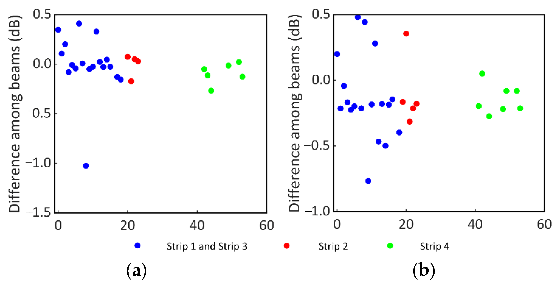
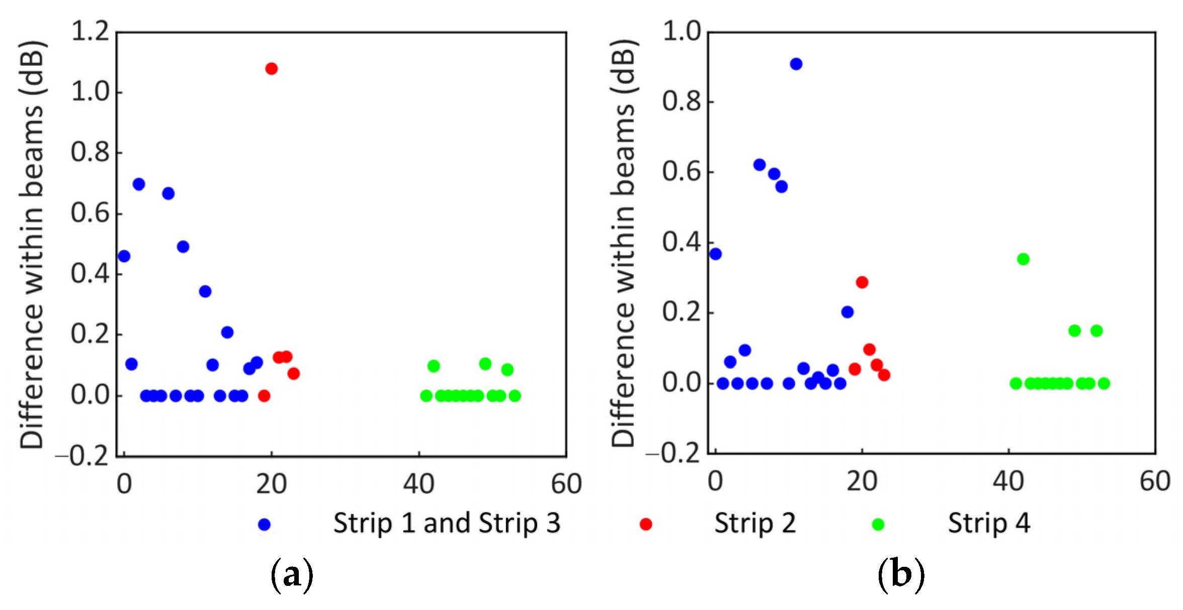
First, we used the proposed method to detect outliers in the absolute calibration constants within beams. By comparing the absolute calibration constants within beams to the mean value of the current beam, as shown in Figure 13, we find that for Strip Mode 2, one absolute calibration constant of beam 20 differs from the mean value by more than 1 dB and is therefore treated as an outlier; the results are shown in

Table 4. Absolute calibration constants of LT-1A satellite from 2023 to 2025 after refinement.

Imaging Mode	Polarization	Absolute Calibration Constants/dB
		2023		2024		2025
		Mean	Standard Deviations	Mean	Standard Deviations	Mean	Standard Deviations
Strip Modes 1 and 3	HH	6.97	0.10	6.57	0.43	6.75	0.27
Strip Mode 2	HH	7.10	0.15	6.85	0.02	—	—
Strip Mode 4	HH	7.11	0.06	7.03	0.03	6.96	0.06
Strip Mode 4	VV	6.77	0.17	6.80	0.38	6.87	0.20

. The standard deviation for Strip Mode 2 in 2024 decreases markedly.

Further analysis of the gain difference among different beams is shown in Figure 14. From Figure 14, we can see that absolute calibration constants of beam 8 for the LT-1A satellite remain consistent after multiple observations, while the difference between beam 8 and other beams exceeds 1 dB. Therefore, we concluded that the gain difference error of beam 8 was above the threshold. Based on the differences in absolute calibration constants between beam 8 and other beams, the gain difference in Beam 8 was corrected by 1.03 dB. We can see that the difference in all beams for the LT-1B satellite are below the limit. We analyzed the absolute calibration constants of the LT-1A satellite after optimization, as shown in Table 4. The averaged values for 2023, 2024, and 2025 are 7.02 dB, 6.79 dB, and 6.80 dB, respectively. These deviations are significantly smaller than pre-improvement. The average absolute calibration constant for the LT-1A satellite is 6.90 dB, with a standard deviation is 0.25 dB (1σ). Absolute radiometric accuracy is improved from 0.40 dB (1σ) to 0.25 dB (1σ). The absolute calibration constants of the LT-1B satellite do not meet the conditions for optimization. With the long-term stability of the SAR satellite, continuous correction of gain differences and anomalies within beams can further refine absolute calibration constants and improve radiometric accuracy.

5. Discussion

In this experiment, we used internal calibration data and field calibration data from the LT-1 satellites collected between 2023 and 2025. After performing pulse compression on the internal calibration data, we monitored the amplitude and phase changes in the TRM internal calibration. The internal calibration results indicate that the TRM calibration shows a slight decrease.

Using the proposed method, we optimized the absolute calibration constant of LT-1A, improving the absolute calibration accuracy. The LT-1B satellite did not meet the criteria and therefore was not corrected. Considering Strip Modes 1, 2, 3, and 4 individually, the absolute calibration constants of the LT-1A satellite exhibit no substantial change, whereas the absolute calibration constants of the LT-1B satellite show a slight decline. The average absolute calibration constant for the LT-1A satellite is 6.90 dB, with a standard deviation of 0.25 dB (1σ), while the average absolute calibration constant for LT-1B is 6.82 dB, with a standard deviation of 0.38 dB. The field calibrations demonstrate that the annual absolute calibration constants of the LT-1 satellites exhibit only minor year-to-year variations. From Table 2, Table 3 and Table 4, an annual standard deviation greater than 0.40 dB may indicate absolute calibration constant outliers or the presence of a gain difference error among beams. The annual standard deviation of Strip Mode 1 for LT-1B in 2025 exceeds 0.40 dB, primarily because one of the absolute calibration constants for beam 9 is 8.13 dB, which differs from others substantially, yet does not meet the correction criteria. The exceedance of the annual standard deviation for LT-1A in 2024 over 0.40 dB is attributed to the limited acquisition of only four datasets under Strip Mode 1.

The amplitude of the TRM transmission channel for the LT-1A/LT-1B satellites exhibits a slight annual decline, with the decrease being marginally greater for LT-1B than for LT-1A. From the year-to-year trends of the absolute calibration constants, no discernible change is observed for LT-1A, while LT-1B shows a slight decline. These findings indicate that, within a certain range, the decrease in internal calibration does not lead to changes in radiometric accuracy. The variation relationship between the internal calibration TRM and the absolute calibration constants requires further investigation.

6. Conclusions

Radiometric calibration establishes the functional relationship between the intensity of the SAR image and the backscattering coefficient of ground targets, enabling the retrieval of quantitative parameters. Field radiometric calibration yields absolute calibration constants but suffers from limited beam coverage. By contrast, internal on-board calibration tracks relative changes in radiometric performance and cannot provide absolute calibration constants. This paper presents a radiometric performance monitoring method for LT-1 SAR satellites combing on-board internal calibration with field calibration. It gives a reference for radiometric performance monitoring of the SAR satellite over a long period. Monthly monitoring of internal calibration in Strip Mode 1 is achieved. Continuous acquisition of field calibration data can confirm the deviations and improve the radiometric accuracy of LT-1 satellites when the SAR payload decreases slightly. In the following work, we will continue to collect both internal calibration data and field calibration data. When the amplitude of the internal calibration decreases gradually while the absolute calibration constant shows no significant change, we can remove outliers within beams and correct gain differences among different beams. At the same time, we will further investigate the impact of variations in the internal calibration on the absolute calibration constants.

References

1. Yang, S.; Li, S.; Wu, W.; Cui, Y.; Liu, M. Capacity analysis of GF-3 satellite on disaster management. Spacecr. Eng. 2017, 26, 155–160. [Google Scholar] [CrossRef]
2. Lin, M.; Yuan, X.; Liu, J.; Ye, X.; Zhang, Q.; Zhao, L.; An, D.; Peng, Y. Application of GF-3 satellite monitoring typhoon. Spacecr. Eng. 2017, 26, 167–171. [Google Scholar] [CrossRef]
3. Tang, X.; Li, T.; Zhang, X.; Zhou, X.; Lu, J.; Zhang, X. In-orbit application parameters test and analysis of L-band differential interferometric SAR satellite constellation. Acta Geod. Cartogr. Sin. 2024, 53, 1863–1872. [Google Scholar]
4. Tang, X.; Li, T.; Zhou, X.; Lu, J.; Zhang, X. National sea area use dynamic monitoring based on GF-3 SAR imagery. J. Radars 2017, 6, 456–472. [Google Scholar]
5. Li, T.; Tang, X.; Li, S.; Zhou, X.; Zhang, X.; Xu, Y. Classification of basic deformation products of L-band differential interferometric SAR satellite. Acta Geod. Cartogr. Sin. 2023, 52, 769–779. [Google Scholar] [CrossRef]
6. Freeman, A. SAR calibration: An overview. IEEE Trans. Geosci. Remote Sens. 1992, 30, 1107–1121. [Google Scholar] [CrossRef] [Scilit]
7. Shi, L.; Sun, W.; Yang, L.; Yang, J.; Zhao, L.; Li, P.; Liu, Y. Evaluation of radiometric and polarimetric errors in the LT-1A satellite data based on tropical forests in the amazon. J. Radars 2025, 14, 405–423. [Google Scholar] [CrossRef]
8. Tous-Ramon, N.; Schrank, D.; Bachmann, M.; Alfonzo, G.C.; Polimeni, D.; Boer, J.; Schwerdt, M. long-term system monitoring status of the TerraSAR-X and the TanDEM-X satellites. In Proceedings of the 9th European Conference on Synthetic Aperture Radar, Nuremberg, Germany, 23–26 April 2012; pp. 1–4. [Google Scholar]
9. Schwerdt, M.; Schmidt, K.; Klenk, P.; Tous Ramon, N.; Rudolf, D.; Raab, S.; Weidenhaupt, K.; Reimann, J.; Zink, M. Radiometric Performance of the TerraSAR-X Mission over More Than Ten Years of Operation. Remote Sens. 2018, 10, 754. [Google Scholar] [CrossRef] [Scilit]
10. Brautigam, B.; Schwerdt, M.; Bachmann, M. An efficient method for performance monitoring of active phased array antennas. IEEE Trans. Geosci. Remote Sens. 2009, 47, 1236–1243. [Google Scholar] [CrossRef] [Scilit]
11. Braeutigam, B.; Gonzalez, J.H.; Schwerdt, M.; Bachmann, M. Radar instrument calibration of TerraSAR-X. In Proceedings of the 7th European Conference on Synthetic Aperture Radar, Friedrichshafen, Germany, 2–5 June 2008; pp. 1–4. [Google Scholar]
12. Schwerdt, M.; Schrank, D.; Bachmann, M.; Schulz, C.; Döring, B.; Gonzalez, J.H. TerraSAR-X re-calibration and dual receive antenna campaigns performed in 2009. In Proceedings of the 8th European Conference on Synthetic Aperture Radar, Aachen, Germany, 7–10 June 2010; pp. 1–4. [Google Scholar]
13. Hajduch, G.; Vincent, P.; Cordier, K.; Husson, R.; Peureux, C.; Schmidt, K.; Piantanida, R.; Recchia, A.; Franceschi, N.; Mouche, A.; et al. S-1A & S-1B Annual Performance Report 2021. Available online: https://sentiwiki.copernicus.eu/__attachments/1681272/DI-MPC-APR-SAR-MPC-0523%20-%20Sentinel-1A%20and%201B%20Annual%20Performance%20Report%202021%20-%201.1.pdf?inst-v=69bf4b9c-8e6b-4a6e-a48c-ce04b3651efe (accessed on 16 April 2026).
14. Hajduch, G.; Vincent, P.; Cordier, K.; Grignoux, M.; Husson, R.; Peureux, C.; Benchaabane, A.; Johnsen, H.; Piantanida, R.; Recchia, A.; et al. S-1 Annual Performance Report 2024. Available online: https://sentiwiki.copernicus.eu/__attachments/1681272/DI-MPC-APR-0715%20-%20Sentinel-1%20Annual%20Performance%20Report%202024%20-%202.1.pdf?inst-v=69bf4b9c-8e6b-4a6e-a48c-ce04b3651efe (accessed on 16 April 2026).
15. Hajduch, G.; Vincent, P.; Cordier, K.; Grignoux, M.; Husson, R.; Peureux, C.; Benchaabane, A.; Johnsen, H.; Piantanida, R.; Recchia, A.; et al. S-1 Annual Performance Report for 2022. Available online: https://sentiwiki.copernicus.eu/__attachments/1681272/DI-MPC-APR-SAR-MPC-0588%20-%20Sentinel-1%20Annual%20Performance%20Report%202022%20-%201.3.pdf?inst-v=69bf4b9c-8e6b-4a6e-a48c-ce04b3651efe (accessed on 16 April 2026).
16. Schwerdt, M.; Schmidt, K.; Tous Ramon, N.; Klenk, P.; Yague-Martinez, N.; Prats-Iraola, P.; Zink, M.; Geudtner, D. Independent System Calibration of Sentinel-1B. Remote Sens. 2017, 9, 511. [Google Scholar] [CrossRef] [Scilit]
17. Schmidt, K.; Tous-ramon, N.; Schwerdt, M. Radiometric accuracy and stability of sentinel-1A determined using point targets. Int. J. Microw. Wirel. Technol. 2018, 10, 538–546. [Google Scholar] [CrossRef] [Scilit]
18. Klenk, P.; Schmidt, K.; Giez, J.; Pulella, A.; Nannini, M.; Prats-Iraola, P.; Schwerdt, M. Independent SAR System Calibration of Sentinel-1C. IEEE J. Sel. Top. Appl. Earth Obs. Remote Sens. 2026, 19, 15833–15853. [Google Scholar] [CrossRef] [Scilit]
19. Liu, B.; Zhang, L.; Ge, D.; Li, M.; Zhou, X.; Guo, Z.; Shi, P.; Zhang, L.; Jin, D.; Wan, X.; et al. Application of InSAR monitoring large deformation of landslides using Lutan-1 constellation. Geomat. Inf. Sci. Wuhan Univ. 2024, 49, 1753–1762. [Google Scholar] [CrossRef]
20. Wang, R.; Liu, K.; Liu, D.; Ou, N.; Yue, H.; Chen, Y.; Yu, W.; Liang, D.; Cai, Y. LuTan-1 An innovative L-band spaceborne bistatic interferometric synthetic aperture radar mission. IEEE Geosci. Remote Sens. Mag. 2025, 13, 58–78. [Google Scholar] [CrossRef] [Scilit]
21. Cumming, I.G.; Wong, F.H. Digital Processing of Synthetic Aperture Radar Data: Algorithms and Implementation; Artech House: Norwood, MA, USA, 2005. [Google Scholar]
22. Miranda, N.; Meadows, P.J. Radiometric Calibration of S-1 Level-1 Products Generated by the S-1 IPF. Available online: https://sentiwiki.copernicus.eu/__attachments/1673968/ESA-EOPG-CSCOP-TN-0002%20-%20Sentienl-1%20Radiometric%20Calibration%20of%20Products%202015%20-%201.0.pdf?inst-v=69bf4b9c-8e6b-4a6e-a48c-ce04b3651efe (accessed on 16 April 2026).
23. ICEYE Data Calibration and Validation. Available online: https://www.iceye.com/hubfs/Downloadables/ICEYE_calibration_and_validation_brochure_June_2020.pdf (accessed on 16 April 2026).
24. Huang, Q.; Zhang, F.; Li, L.; Liu, X.; Jiao, Y.; Yuan, X.; Li, H. Quick Quality Assessment and Radiometric Calibration of C-SAR/01 Satellite Using Flexible Automatic Corner Reflector. Remote Sens. 2023, 15, 104. [Google Scholar] [CrossRef] [Scilit]
25. Yao, Y.; Han, Q.; Xu, Z.; Wang, A.; Zhao, H.; Yan, L. Radiometric calibration and cross calibration of HJ-2 06 satellite based on point targets. Nat. Remote Sens. Bull. 2025, 29, 3327–3335. [Google Scholar] [CrossRef] [Scilit]
26. Ou, N.; Bai, M.; Liang, B.; Miao, J. Application of the trihedral corner reflector in RCS calibration test. J. Beijing Univ. Aeronaut. Astronaut. 2013, 39, 220–224. [Google Scholar]
27. Dell’Amore, L.; Bueso–Bello, J.; Klenk, P.; Reimann, J.; Rizzoli, P. Characterization of the Amazon Rainforest Backscatter at X-Band Using TanDEM-X Data. IEEE J. Sel. Top. Appl. Earth Obs. Remote Sens. 2024, 17, 1673–1690. [Google Scholar] [CrossRef] [Scilit]
28. Yao, Y.; Zhao, H.; Han, Q.; Yang, B.; Wang, A. Research on Radiometric Calibration Constant Optimization of GF-3 Satellite Based on Onboard Internal Calibration. Spacecr. Eng. 2025, 34, 150–159. [Google Scholar]
29. Gao, C.; Deng, Y.; Feng, J. Influences of mismatch on the multi-channel synthetic-bandwidth SAR system and the corresponding correction measure. J. Electron. Inf. Technol. 2012, 34, 154–159. [Google Scholar]
Figure 1. Distribution map of the corner reflectors in the calibration site. (a) Distribution map of the corner reflectors from CR-1 to CR-23; (b) Distribution map of the corner reflectors from CR-24 to CR-31.
Remotesensing 18 01856 g001
Figure 2. Flowchart of the radiometric performance monitoring method for the LT-1 satellites based on internal calibration and field calibration.
Remotesensing 18 01856 g002
Figure 3. Flowchart of absolute calibration constant calculation.
Remotesensing 18 01856 g003
Figure 4. Definitions of the point target impulse response region and the background region.
Remotesensing 18 01856 g004
Figure 5. Flowchart of absolute calibration constant refinement and absolute radiometric accuracy evaluation.
Remotesensing 18 01856 g005
Figure 6. Trends of the TRM transmitting channels and the TRM receiving channels of the LT-1A satellite at beam 6 (different colored curves represents different channels). (a) Amplitude trend of the transmitting channels. (b) Phase trend of the transmitting channels. (c) Amplitude trend of the receiving channels. (d) Phase trend of the receiving channels. (e) Amplitude difference between channel 1 and channel 2. (f) Phase difference between channel 1 and channel 2.
Remotesensing 18 01856 g006aRemotesensing 18 01856 g006b
Figure 7. Trends of the TRM transmitting channels and receiving channels of the LT-1B satellite at beam 6 (different colored curves represents different channels). (a) Amplitude trend of the transmitting channels. (b) Phase trend of the transmitting channels. (c) Amplitude trend of the receiving channels. (d) Phase trend of the receiving channels. (e) Amplitude difference between channel 1 and channel 2. (f) Phase difference between channel 1 and channel 2.
Remotesensing 18 01856 g007
Figure 8. Trends of the TRM transmitting channels and receiving channels of the LT-1A satellite at beam 8 (different colored curves represents different channels). (a) Amplitude trend of the transmitting channels. (b) Phase trend of the transmitting channels. (c) Amplitude trend of the receiving channels. (d) Phase trend of the receiving channels. (e) Amplitude difference between channel 1 and channel 2. (f) Phase difference between channel 1 and channel 2.
Remotesensing 18 01856 g008
Figure 9. Trends of the TRM transmitting channels and receiving channels of the LT-1B satellite at beam 8 (different colored curves represents different channels). (a) Amplitude trend of the transmitting channels. (b) Phase trend of the transmitting channels. (c) Amplitude trend of the receiving channels. (d) Phase trend of the receiving channels. (e) Amplitude difference between channel 1 and channel 2. (f) Phase difference between channel 1 and channel 2.
Remotesensing 18 01856 g009aRemotesensing 18 01856 g009b
Figure 10. Variation trends of TRM transmitting channels’ amplitude (different colored curves represents different channels). (a) Beam 6 of LT-1A satellite. (b) Beam 8 of LT-1A satellite. (c) Beam 6 of LT-1B satellite. (d) Beam 8 of LT-1B satellite.
Remotesensing 18 01856 g010aRemotesensing 18 01856 g010b
Figure 11. Signal-to-clutter ratios for different beams. (a) LT-1A. (b) LT-1B.
Remotesensing 18 01856 g011
Figure 12. Results of the main lobe energy ratios for different beams. (a) LT-1A. (b) LT-1B.
Remotesensing 18 01856 g012
Figure 13. Absolute calibration constant differences within beams of LT-1 satellite. (a) LT-1A. (b) LT-1B.
Remotesensing 18 01856 g013
Figure 14. Absolute calibration constant differences among different beams of LT-1 satellite. (a) LT-1A. (b) LT-1B.
Remotesensing 18 01856 g014