Article

Estimating Canopy Structure Parameters and Leaf Nitrogen in Olive Orchards Using UAV Imagery Across Two Agro-Ecological Zones in Tunisia

1
FG Agromechatronik, Institut für Maschinenkonstruktion und Systemtechnik, Technische Universität Berlin, Straße des 17. Juni 144, 10623 Berlin, Germany
2
Leibniz-Institut für Agrartechnik und Bioökonomie e.V., Department of Agromechatronics, Max-Eyth-Allee 100, 14469 Potsdam, Germany
3
Olive Institute, Unit of Sousse, Ibn Khaldoun BP 14, Sousse 4061, Tunisia
4
Department of Agricultural Sciences, BOKU University, 1180 Vienna, Austria
*
Author to whom correspondence should be addressed.
Remote Sens. 2026, 18(9), 1300; https://doi.org/10.3390/rs18091300
Submission received: 23 February 2026 / Revised: 20 April 2026 / Accepted: 20 April 2026 / Published: 24 April 2026

Highlights

What are the main findings?
  • First photogrammetrical study on UAV-based monitoring for orchards of local Tunisian olive varieties (Olea europaea L. cv. Chetoui, Olea europaea L. cv. Chemlali).
  • Individual tree structural parameters (height, crown volume, projected crown area, and LAI) can be delineated in a challenging context (sparse foliage, low-cost approach, and low-altitude flight setting).
  • Leaf chlorophyll/nitrogen values cannot be delineated using low-cost RGB sensors.
What are the implications of the main findings?
  • Low-altitude, UAV-based photogrammetry can set a basis for precise olive orchard monitoring in Tunisia.
  • The low-cost approach focusing on local varieties raises the interest of local farmers in UAV adoption.

Abstract

Optimizing olive orchard management requires timely, per-tree data to enhance productivity and sustainability. Unoccupied aerial vehicle (UAV)-based red, green, and blue (RGB) imagery offers a low-cost solution for acquiring high-resolution spatiotemporal insights for orchard management, which are not yet common in Tunisia. This study monitored tree structural parameters, leaf area index (LAI), and leaf nitrogen content (%N DW) in two Tunisian olive orchards during 2022 and 2023. UAV-derived imagery was photogrammetrically processed into 3D point clouds and analyzed using an automated approach. Target variables of the automated approach included tree-wise estimates of height, projected crown area, and crown volume, as well as raster cell counts of the canopy cloud and spectral indices such as the normalized green-red difference index (NGRDI) and green leaf index (GLI). In addition, the estimated parameters per tree were used to model LAI and leaf nitrogen content. Analyses were conducted separately for trees represented by a high and a low number of points in the dense point cloud. Outcomes were compared to reference data collected in the field on dates close to the UAV flights. The findings showed strong relationships for the projected crown area (R2 = 0.82 and 0.91) and tree height (R2 = 0.89 and 0.88) when compared to reference values. Linear regression models for LAI (R2 = 0.73 and 0.68) and crown volume (R2 = 0.85 and 0.91) estimation also show strong relationships. However, leaf nitrogen estimation was not feasible from RGB spectral index values, as it showed a weak relationship (R2 = 0.34). A dataset with multispectral imagery could overcome this limitation but would increase costs, making it less suitable for the low-budget approach required in price-sensitive farming contexts, particularly in low-income regions.

1. Introduction

In Tunisia, olives represent the most extensively cultivated fruit crop with around 107 million trees covering two million hectares of land, according to the Tunisian Ministry of Agriculture, Hydraulic Resources, and Fisheries. Traditionally, olive trees in Tunisia have been grown under rainfed conditions. However, the country is increasingly grappling with severe water scarcity. At the same time, decreasing soil organic matter contents have been observed due to unsustainable land use practices and the intensifying effects of climate change [1,2,3]. Different farm management practices and systems, such as organic farming, have been shown to alleviate some of the negative effects, e.g., refs. [4,5,6,7].
To give local farmers the option to react to resource scarcity and better understand plant parameter distributions over olive groves, it is essential to obtain spatial information at the scale of individual trees. In order to actually have an influence on agricultural management, the monitoring approach should be tested on local varieties, using low-cost technologies, and should work within a reasonable amount of time. This would allow for management practices tailored to the needs of single trees based on their specific location and conditions.
Precision agriculture represents a suitable strategy for responding to dynamic and spatially different crop demands and for implementing integrated land, soil, water, nutrient, and crop management approaches. In this context, remote- and proximal-sensing tools have proven to be widely efficient for the detection and management of water stress, e.g., ref. [8], and nutrient deficiencies, e.g., ref. [9], at the field level and across large-scale regions. Policymakers, stakeholders, and end-users highlighted the importance of sensing technologies in assisting farmers to adopt sustainable agricultural practices, optimize irrigation and nutrient inputs, and achieve profitable returns [10,11,12].
Canopy structure and tree vitality strongly influence the overall performance of an olive tree in terms of fruit yield and quality [13]. The leaf area index (LAI), a tree structural parameter that represents the leaf area per unit of ground surface, is interrelated with tree growth, light interception, and evapotranspiration [14]. By monitoring LAI, farmers can make informed decisions about irrigation, fertilization [15], crop protection [16], or pruning at the right time [17]. However, measuring LAI involves destructive and laborious sampling of leaves from each tree, making it infeasible to apply across an entire olive grove. An alternative is to use the gap-fraction method, which can be conducted from rough farmers’ estimations [18] or, more commonly, from sensor-based measurements [19]. This method involves measuring the proportion of gaps in canopy cover to assess the LAI with radiation transfer models. Leaf chlorophyll is closely correlated with the photosynthetic performance and nitrogen status of a tree and therefore links to crop stresses caused by factors like malnutrition, disease, or drought [20]. Portable chlorophyll meters offer fast, non-destructive measurements of the chlorophyll index and leaf nitrogen status directly on the leaves using the light transmission method [21]. It was effectively tested on olive trees by Boussadia et al. [22]. However, ground-based sensor measurement still implies re-visiting each tree or may underperform because only a fraction of the tree can be measured, e.g., a certain number of leaves.
Remote sensing tools can provide reliable spatial information about tree performance across an entire orchard. Specifically, unoccupied aerial vehicles (UAVs), or drones, are becoming increasingly common for capturing site-specific information with high spatial resolution and detail. UAV platforms can carry multiple sensors over fields to collect data, bridging the gap between ground-based proximal sensing and satellite-based remote sensing. They are highly adaptable and can be configured for multiple purposes. UAVs allow for flexible camera configurations, especially for RGB (red-green-blue), multispectral (MS), and hyperspectral (HS) cameras and LiDAR scanners. The choice of the sensor’s configuration depends on the management or research aim and is influenced by technical specifications such as resolution, optical quality, weight, number of images, and cost [23]. This flexibility is useful when considering different UAV flight planning trade-offs for agricultural purposes. For example, the need to cover medium-sized and large orchard areas with limited battery capacity may require high-altitude, nadir flight settings that provide wide coverage with each image, while low-altitude, oblique flight settings provide an enhanced resolution [24] and a more relevant angle of view to detect features of interest hidden under the canopy [25]. In addition, processing time can be a limiting factor. The ability of UAV platforms to adjust altitude offers high flexibility in meeting specific orchard requirements and resolutions. In combination with efficient structure-from-motion algorithms, ortho-images or three-dimensional surface models can be photogrammetrically created from many aerial images. This approach benefits strongly from higher image overlap, which can be achieved through higher flight altitudes or slower vehicle velocities, assuming the same sensor. This is particularly relevant for delineating structural tree parameters, as shown by Torres-Sanchez et al. [26]. However, the optimal flight settings depend on the target parameter. For instance, an optimal forward overlap of 80% and 95% has been found to be most beneficial for estimating tree height and tree crown volume in olive orchards, respectively [26]. Such information provides insights into plant status and future yield, as noted by Yang et al. [27]. Studies have demonstrated the delineation of tree structural parameters, such as crown area and tree height [27,28,29], tree crown volume [30], and the distribution of plant performance parameters, such as LAI [31,32,33,34] and leaf or plant nitrogen status derived from RGB data for various crops [35,36,37,38,39]. However, leaf nitrogen delineation from RGB imagery can be challenging, as color bands in this kind of sensor are broad and do not cover spectral ranges that are more responsive to this plant parameter, like red edge and near infrared. Moreover, when a bright background shines through the canopy, it can influence captured neighbor pixels, leading to a contaminated mixed signal.
The use of UAVs has the potential to benefit olive farming in Tunisia. Olive orchard systems in Tunisia typically consist of tree rows with interstitial space in between plant canopies of multiple meters forming isolated tree stands, which result in more complex three-dimensional structures compared to tree row systems with a closed canopy. In addition, these orchards are usually too large to be monitored with ground-based sensors at high temporal resolutions. In contrast, UAVs can provide detailed spatial information across entire orchards with high spatial resolutions. However, legal hurdles complicate the use of UAVs for agricultural and scientific purposes, which may explain the limited application in agricultural practice and research of this technology in Tunisia. A search of the ISI database (as of 28 March 2025; 09:30 am) revealed only two publications that combine the keywords ‘olive’, ‘UAV’, and ‘Tunisia’. The keyword ’Tunisia’ in this context refers to the locations of institutes contributing to the publications, not the location of the field trials. Massaoudi et al. [40] investigated a theoretical responsive irrigation system in olive orchards with UAV-based monitoring to assess soil conditions such as temperature, humidity, light, soil moisture, and nutrient levels. Their study proposed that UAVs could also monitor crop health and detect anomalies in orchards. The authors argued that integrating UAV monitoring into a responsive network system could integrate smart farming practices in Tunisian irrigation systems and lead to savings in scarce irrigation water. Another study used deep learning techniques to detect and classify olive leaf diseases in field trials conducted in Saudi Arabia [41]. Hence, the use of UAVs in Tunisian olive cultivation is still under-represented, and tree parameter delineation for local varieties has not yet been actively researched.
Currently, targeted monitoring of olive orchards relies on ground-based assessments, which are time-consuming and labor-intensive. To improve the efficiency and spatial resolution of orchard monitoring, the application of remote sensing technologies, particularly UAVs, should be promoted by more research field studies on local varieties and field conditions. In this study, two local varieties, namely Olea europaea L. cv. Chetoui and Olea europaea L. cv. Chemlali, were researched using UAV remote sensing. We aimed at a fully automated approach to delineate tree-wise structural parameters and leaf chlorophyll directly from the point cloud models. There are some specifics to this research study that should be mentioned beforehand. Firstly, the plant setting of both researched sites was single-standing trees, as they are common in Tunisia, and the local varieties do not form a closed canopy. This leads to the situation where bright ground reflections are visible between trees and partially through the canopy in the imagery taken from a nadir perspective, and they may saturate or obscure thin branches and leaves. Secondly, flight campaigns were done at a low-altitude, which increases the resolution in the tree canopy but, at the same time, increases relative positional changes of branches close to the lens in the overlapping images. Finally, we set the constraint that only a low-cost RGB camera sensor was used for data capturing. This may promote the use of UAVs for olive orchard monitoring by local farmers, because the technology used is more affordable. However, this comes at the cost of reduced image quality and spectral range.
Specifically, this research study was conducted to address the following research questions for two local olive varieties:
  • Can UAV-derived RGB point clouds be used to automatically assess tree canopy structures for Tunisian olive varieties?
  • Is it feasible to estimate physiological parameters, such as the leaf area index (LAI) or leaf chlorophyll content, at the individual tree level?
  • Do the generated maps of the investigated parameters provide sufficient spatial detail to support detailed assessments of orchard conditions?

2. Materials and Methods

2.1. Approach

This field study focused on plant parameters related to olive canopy structure and leaf physiological conditions monitored using UAV-based RGB imagery. In two olive tree orchards located in different agroecological zones, UAV flights were conducted across two seasons. The collected imagery was used to photogrammetrically delineate three-dimensional point cloud models from the orchards, which were analyzed for tree height, projected crown area over ground, crown volume, and a count of raster cells that include at least one point of the analyzed tree. Additionally, the spectral indices NGRDI and GLI were calculated per tree. The crown volume and raster cell count were further used to estimate the LAI per tree. The spectral indices were used to estimate the leaf nitrogen content of the canopy. To achieve this, a script was developed, based on a previous version used by Hobart et al. [42], which was updated and more advanced for automated tree parameter analysis directly from three-dimensional point clouds. For ground truthing, ground-based photographs were used to measure tree height. LAI measurements were captured with a canopy meter (LAI-2200C Plant Canopy Analyzer, Li-COR Bioscience, Bad Homburg v. d. Höhe, Germany) and post-processed, providing values for crown volume and the projected crown area. Moreover, leaf chlorophyll content was measured with a SPAD meter, and values were averaged per tree and calibrated with laboratory measurements for the nitrogen content of collected leaves. The estimated parameters were used to create tree-wise status maps. The results are presented as spatial distributions of the estimated parameters in maps and validated against ground-based reference values or using cross-validation.

2.2. Study Site

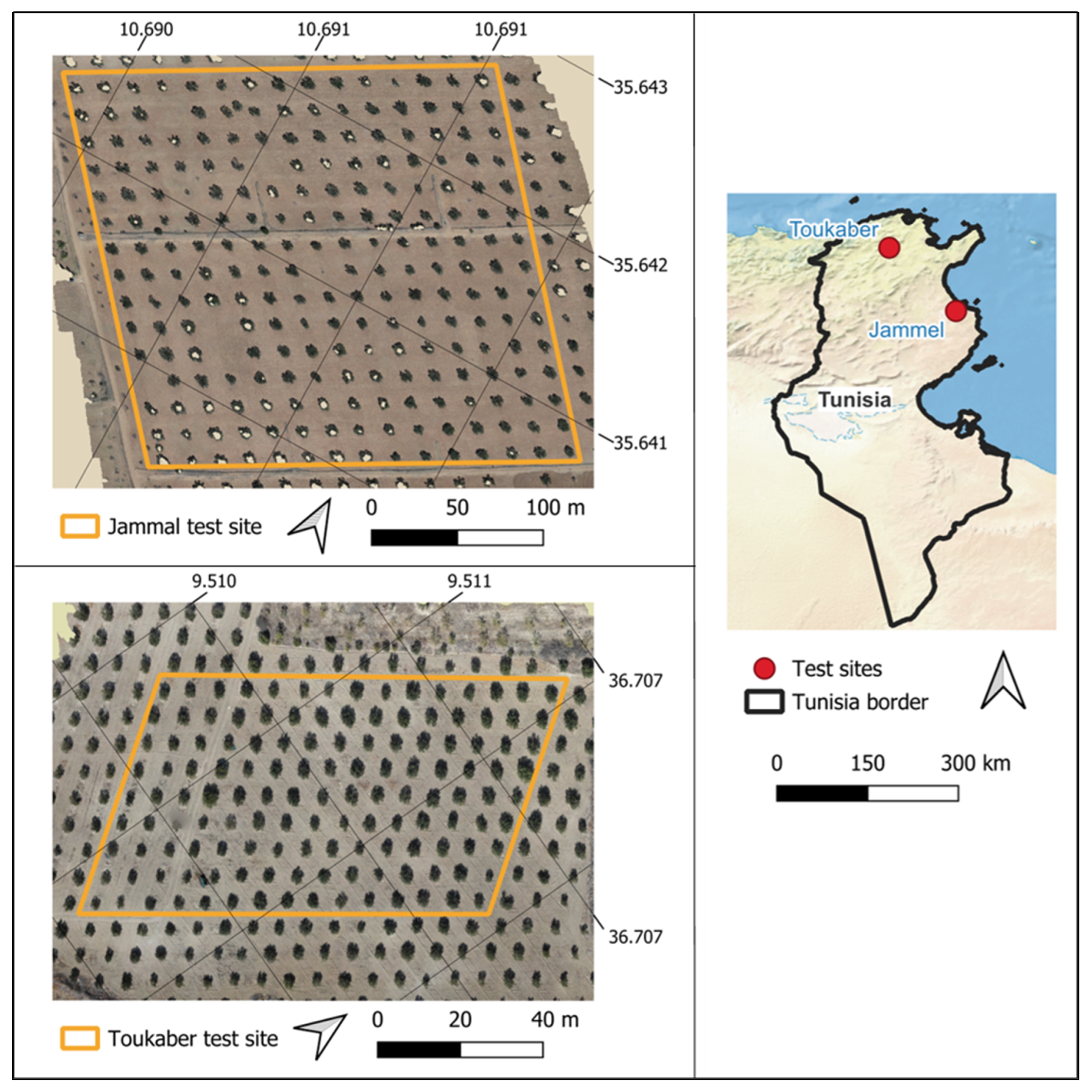
This study was conducted during the 2022 and 2023 cropping seasons at two experimental sites in Tunisia, as shown in Figure 1. These seasons represent a high-yield and a low-yield year for the alternate-bearing olive cultivars. The first site was located at an organic farm in Toukaber (36°42′22″N 9°30′38″E, Beja Governorate, Tunisia). This orchard consists of mature olive trees (Olea europaea L. cv. Chetoui) with a tree age of 20 years planted with a spacing of 8 m × 8 m, with 135 olive trees occupying about 0.73 ha. The ‘Chetoui’ is a traditional Tunisian cultivar valued for its high oil content and strong oxidative stability, and it is commonly grown in the northern regions of the country. The climate in this region is typically Mediterranean, with an average annual rainfall of 550 mm, concentrated mainly from fall to spring, and an average annual temperature of 18 to 20 °C.
The second site was a rain-fed organic olive orchard (Olea europaea L. cv. Chemlali) located at the experimental farm of Jammel Agricultural Vocational Training Center (35°38′27.5″N 10°41′24.2″E, Governorate of Monastir, Tunisia). The ‘Chemlali’ variety is cultivated in Tunisia for oil production, often in organic farming systems. The trees at this site are 70 years old and were planted at a spacing of 20 m × 20 m, with 225 olive trees occupying 7.1 ha. The region of Jammel also has a Mediterranean climate but with lower average rainfall of 330 mm year−1, mainly occurring from September to April, and a higher average annual temperature of 22 °C.

2.3. UAV Flight Campaigns

UAV flights were conducted in Jammel on 22 and 28 July 2022 and 3 August 2023, as well as in Toukaber on 29 July 2022 and 5 October 2023. In compliance with regulatory requirements, all UAV operations were conducted in collaboration with the authorized company SONAPROV (The National Plant Protection Company, Mégrine, Tunisia). A DJI Mavic 2 Enterprise Dual (DJI, Shenzhen, China), equipped with a consumer-grade RGB camera, was used for image acquisition. The complete system can be purchased at a price of less than 3000 €, which is considered low-cost compared to UAV combinations with multispectral, hyperspectral, or LiDAR sensor systems. Flights were conducted at an altitude of 30 m, except for the 2023 flight in Toukaber, where the altitude was increased to 40 m to account for sloping terrain. After UAV flights at the Toukaber site in 2022, the number of usable reference trees for SPAD measurements was reduced due to data loss. This data loss occurred as a result of reduced image overlap caused by terrain relief, which minimized the UAV’s distance to the ground and disrupted photogrammetric processing for parts of the orchard. To address this issue, the flight altitude for the Toukaber site was increased to 40 m in the following season. The camera had a 1/2.3” CMOS 12MP sensor chip with a pixel pitch of 1.5 µm, resulting in a ground sampling distance of about 1 cm/px. The image overlap was set to >85%. Because of the different flight altitudes in Toukaber in 2023, the ground sampling distance changed to about 1.3 cm/px, and the image overlap was changed to >90%.
Figure 1. Ortho image of Jammel (top left) and Toukaber (bottom left) test site in 2023, as well as an overview of site locations in Tunisia (right).
Remotesensing 18 01300 g001

2.4. Reference Data

LAI, tree crown volume, and projected crown area over ground were measured for 31 and 29 olive trees at the Jammel and Toukaber orchard sites, respectively, during the 2022 and 2023 growing seasons. These three tree parameters were assessed using the LAI-2200C Plant Canopy Analyzer (LI-COR Inc., Lincoln, NE, USA). The sensor consists of five concentric, conical rings (7°, 23°, 38°, 53°, and 68°) that record the light difference above and below the plant canopy. These measurements are used to calculate the gap fraction, which, after a scatter correction during post-processing (accounting for leaf structure, e.g., clumping effect), provides a non-destructive estimate of LAI.
To estimate a reference LAI, the constrained least squares method (ClsLAI) was applied, as described by Perry et al. [43] and Campbell and Norman [44]. This method uses the projected crown area, rather than crown volume, to derive the reference LAI value. Measurements were conducted, as described in the manual [45], four times per tree in each direction using a 90° cap to ensure full 360° canopy coverage. Each measurement consisted of two readings: one triple light sensor capturing areas below the canopy, which is able to deal with outlier readings, and one single reading in bright sunlight to monitor the light incident on the canopy. The device was initially calibrated before data collection and recalibrated every hour during field measurements.
To determine the actual LAI of the tree, the measured values were analyzed in the following post-processing procedure according to the sensor data analysis manual [46]. Scatter correction, based on Kobayashi et al. [47], was carried out using the FV2200 software (version 2.1.1; LI-COR Biosciences, Inc., Lincoln, NE, USA). This process required the individual definition of a crop or tree model. Using the ‘isolated measured’ option, 11 points were manually determined with a custom script in the Matlab software (version R2025a, The MathWorks, Portola Valley, CA, USA). One point in the image was placed at the ground below the tree, and another was placed at the highest point in the canopy center. The distance between these points was used to calculate the tree height. Six additional points were placed around the tree canopy to define its one-sided shape. Moreover, one point marked the LAI sensor position during measurement, and two additional points were used to define a scale of known distance. All points were manually placed directly onto the images, as illustrated in Figure 2. The plant model generated by the software subsequently estimated the crown volume and area, which served as reference parameters.
To address changing light conditions during field measurements, three calibration measurements were conducted before data collection and repeated every hour, as recommended in the sensor manual [45]. Additionally, obstacle-free reference measurements were taken immediately before below-canopy measurements, maintaining the same view direction. Transmission ratios for the below-canopy measurements were calculated and limited to a factor of 1.0 relative to the reference value, as it is not reasonable for light conditions under the tree to exceed those of a clear sky view. The final post-processed LAI reference value was then calculated and used to fit an LAI model derived from the 3D point clouds.
Leaf nitrogen content was recorded using SPAD value measurements from 25 and 30 trees in Jammel and 23 olive trees in Toukaber during both the 2022 and 2023 growing seasons. At the Toukaber site in 2022, the number of usable reference trees for SPAD measurements was reduced to 17 due to data loss in the point cloud model, as described in Section 2.3 (UAV Flight Campaigns). Therefore, tree parameters in this orchard area could not be delineated for that season.
For assessing the leaf nitrogen content, SPAD values were recorded from 10 leaves of each tree using a SPAD chlorophyll meter (SPAD 502 Plus, Spectrum Technologies Inc., Bridgend, UK). SPAD readings were then calibrated with actual nitrogen content measured in the laboratory. Therefore, an additional set of 20 SPAD leaf measurements was taken from 10 of the previously sampled trees. These leaves were then collected and analyzed for nitrogen content using the Kjeldahl method [48]. A regression model was subsequently developed to estimate the leaf nitrogen content based on SPAD values, following the methodology described by Boussadia et al. [22].

2.5. Data Analysis

A total of 2096 and 1355 RGB images were acquired for the Jammel site, and 153 and 448 images were acquired for the Toukaber site during the 2022 and 2023 UAV campaigns, respectively. The imagery was photogrammetrically processed in the photogrammetric software Metashape (version 1.8.4, Agisoft, Russia). For Jammel, the datasets from both years were aligned with high-accuracy settings. Notably, in 2022, image acquisition at Jammel occurred over two separate dates (22 and 24 July), and the datasets were subsequently merged prior to processing. For Toukaber, all images were aligned with high-accuracy settings for the dataset captured in 2023. The field campaign in 2022 suffered from a partial data loss, as previously described. From the generated sparse clouds, depth maps were calculated with ultra-high accuracy and mild depth filtering, following recommendations published by Tinkham and Swayze [49]. The generated ortho images and 3D dense clouds were reprojected to the UTM coordinate system (EPSG: 32632) and exported for further processing. As part of a preprocessing step, dense clouds were limited to the field borders, and points depicting high obstacles in the field were excluded. To manage memory capacity, dense cloud ground points for Jammel were randomly subsampled to 25% for both years. Photogrammetrical processing was conducted using a workstation with 384 GB of random access memory, an Intel(R) Xeon(R) CPU E5-2667 v4 with 3.20 GHz, and two Quadro P5000 GPUs. Processing times for the sparse cloud creation were in the range from 56 min to 85 min and 24 min, and for dense cloud creation, they were in the range from 10.5 h to 14 h and 7.25 h for the Jammel and Toukaber sites, respectively.
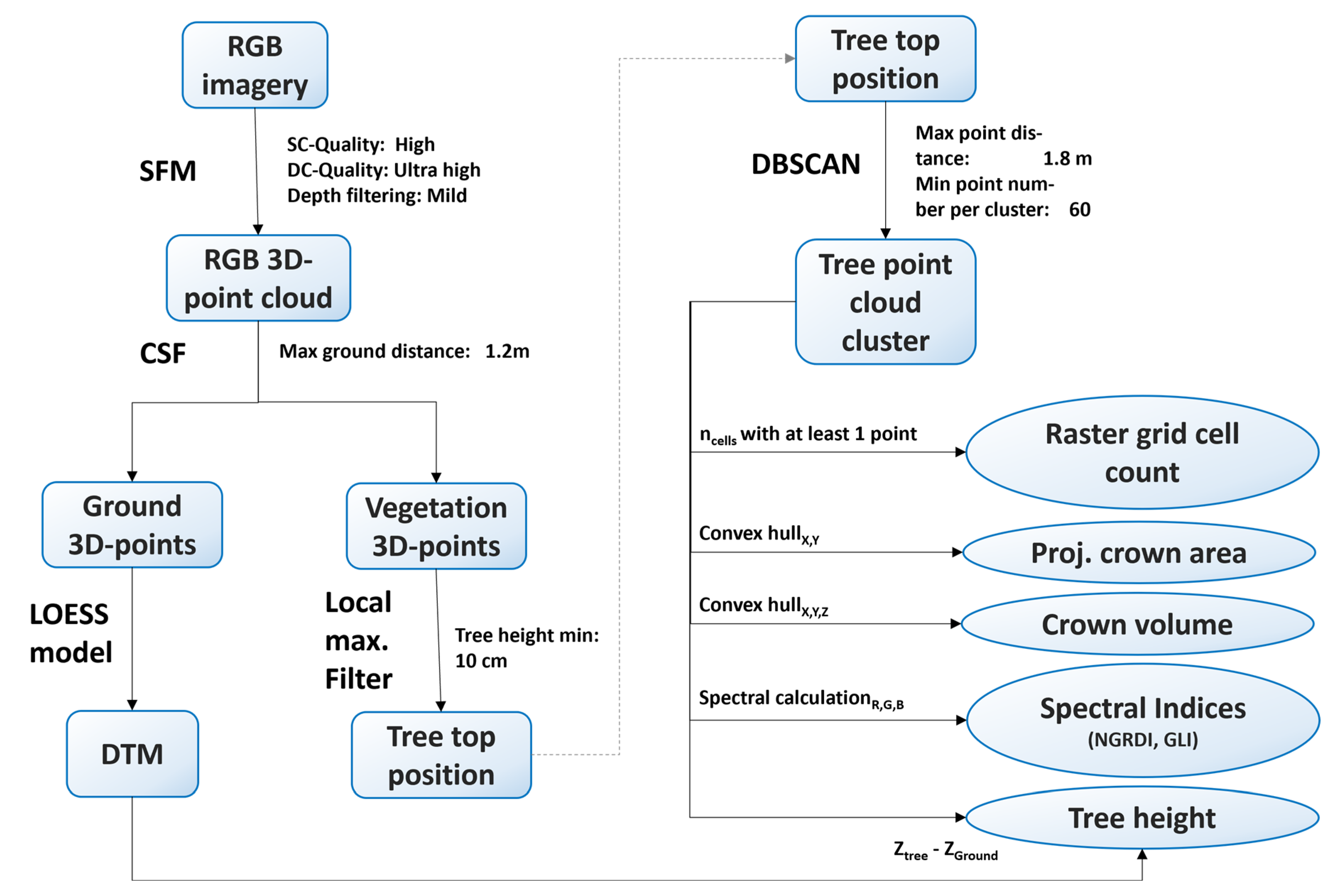
For tree parameter estimation from the dense point cloud models, an enhanced R script (version 4.4.0, R Core Team, R Foundation for Statistical Computing, Vienna, Austria) developed by Hobart et al. [42] was used. The script was modified to estimate spectral and more complex tree parameters, as shown in Figure 3. To identify the trees, the dense point cloud was divided into ground and non-ground points using the cloth simulation filter algorithm [50] within the classify points function from the lidR library [51,52]. Further, the ground points were modelled as a grid with a resolution of 16 points per m2 using a local linear regression model with the loess function [53] from the stats library. All non-ground points were combined in a canopy height model, and individual tree tops were identified using a local maximum filter [54]. Around tree tops, the point cloud was clustered, given that the number of points was at least 60 and the maximal distance in between two points was 1.8 m, using the DBSCAN algorithm [55] from the dbscan library [56,57]. This process created a polynomial ground surface and separated tree clusters.
As a basis for the following tree analysis, four parameters were estimated from the 3D point cloud models. First, the height was modelled from the 95th percentile of the most distant point per tree from the nearest neighbor of the loess grid. Next, the projected crown area over ground and crown volume were calculated using the n-dimensional Quickhull algorithm [58], implemented in the convhulln function from the geometry library [59] for each cluster. Finally, the number of cells from a 3D grid with a 0.05 m × 0.05 m × 0.05 m raster cell size that included at least one point of that tree was delineated.
To estimate individual tree heights, the height values, delineated from the point cloud models, were used for linear regression. During the analysis, an influence on the model along with the number of points representing each tree became apparent, which was causing a difference mainly in the model’s intercept. Therefore, the dataset was split up into two groups following a hierarchical cluster analysis [60] of the logarithmic point number per tree with a threshold of about 4.5. These groups were maintained for all further structural analysis. The resulting models were validated with independent field measurements. Also, the projected crown area over ground, as delineated using the 2D convex hull function of the X and Y coordinates per tree point cluster, was modelled using linear regression and validated with field measurements. For the crown volume per tree, a linear regression of the delineated crown volume, the number of raster cells, and the interaction of these parameters was used. In this study, interactions between variables were calculated as the multiplication of two centered variables, following the standard calculation in statistical software JMP18 (version 18.2.0, Statistical Discovery LLC, Cary, NC, USA). The influence of the parameters on the model was calibrated using the reference measurements. For estimating the LAI, the same two parameters as for the crown volume model were used in a linear regression per tree. The number of cells, crown volume, and their interactions were included in the LAI model. The models for tree crown and LAI were validated using leave-one-out cross-validation (LOOCV) with the statistical programming language R (version 4.4.0) [61]. All structural tree parameters from both sites were combined to achieve a good range of values to create calibration functions, as the structural delineation is considered independent of environmental conditions.
To better fulfil the assumptions of normality and homogeneity of variance for an ordinary regression, the response y was transformed using the Box-Cox-Y transformation [62] with the statistical software JMP (version 18.2.0, Statistical Discovery LLC, Cary, NC, USA). The transformations are given by
y t = y λ 1 λ · y ˙ λ 1 for   λ 0   or
y t = y ˙   · ln ( y ) for   λ = 0
for which y t is the transformed variable, y is the untransformed variable, and y ˙ is the geometrical mean of the variable y. λ is the transformation variable that takes into account the maximum likelihood and minimizes the sum of squared errors. A back transformation of the model predictions was calculated using Equations (3) or (4).
y = ( y t · ( λ · y ˙ λ 1 ) + 1 ) 1 / λ for   λ 0   or
y = e y t y ˙ for   λ = 0
The SPAD value was already linked to leaf chlorophyll and leaf nitrogen content by nonlinear correlation [22]. To model the SPAD value, which depends on leaf nitrogen and chlorophyll content, the normalized green-red difference index (NGRDI), as provided by Tucker et al. [63], was determined by Equation (5) for each point of a tree canopy:
N G R D I = R G r e e n R R e d R G r e e n + R R e d
and the green leaf index (GLI) was determined by Equation 6 for each point in the dense clouds of that tree canopy.
G L I = R G r e e n R R e d R B l u e R G r e e n + R R e d + R B l u e
In Equations (5) and (6), RGreen, RRed, and RBlue refer to the raw digital numbers of the color channels of the RGB camera sensor. Spectral index values were then summarized per tree with descriptive statistical parameters, namely mean, median, both quartiles, and the max and min values. These summarized parameters were used to model a SPAD value per tree in a stepwise forward linear regression.

3. Results

During the field campaigns for the Jammel and Toukaber olive orchards, multiple reference datasets were collected. The mean values of these ground-based reference data are shown in Table 1. Trees in Jammel were taller and more voluminous, exhibiting the shape of fully grown trees. In contrast, olive trees in Toukaber appeared more bush-like, with a smaller height and crown volume. However, despite their smaller size, the LAI was higher for trees at the Toukaber site, indicating a relatively high leaf area for their compact shape.
To monitor tree parameters from the UAV perspective alone, models were developed to estimate the reference variables for each tree without the use of any ground-based parameters. For this, imagery was processed photogrammetrically to dense point clouds. These showed visually comparable results for the Jammel site, independent of the alternating high and low bearing seasons, respectively. For Toukaber, the data loss in 2022 is a visible difference from the 2023 dataset. After a higher flight altitude was set in the following year, data loss was prevented, leading to a slightly decreased ground resolution of 1.3 cm/px compared to 1.0 cm/px in 2022. All created point clouds showed reprojection errors in the range from 0.53 px to 0.63 px. The resulting models for tree parameter estimation are described in the following paragraphs.
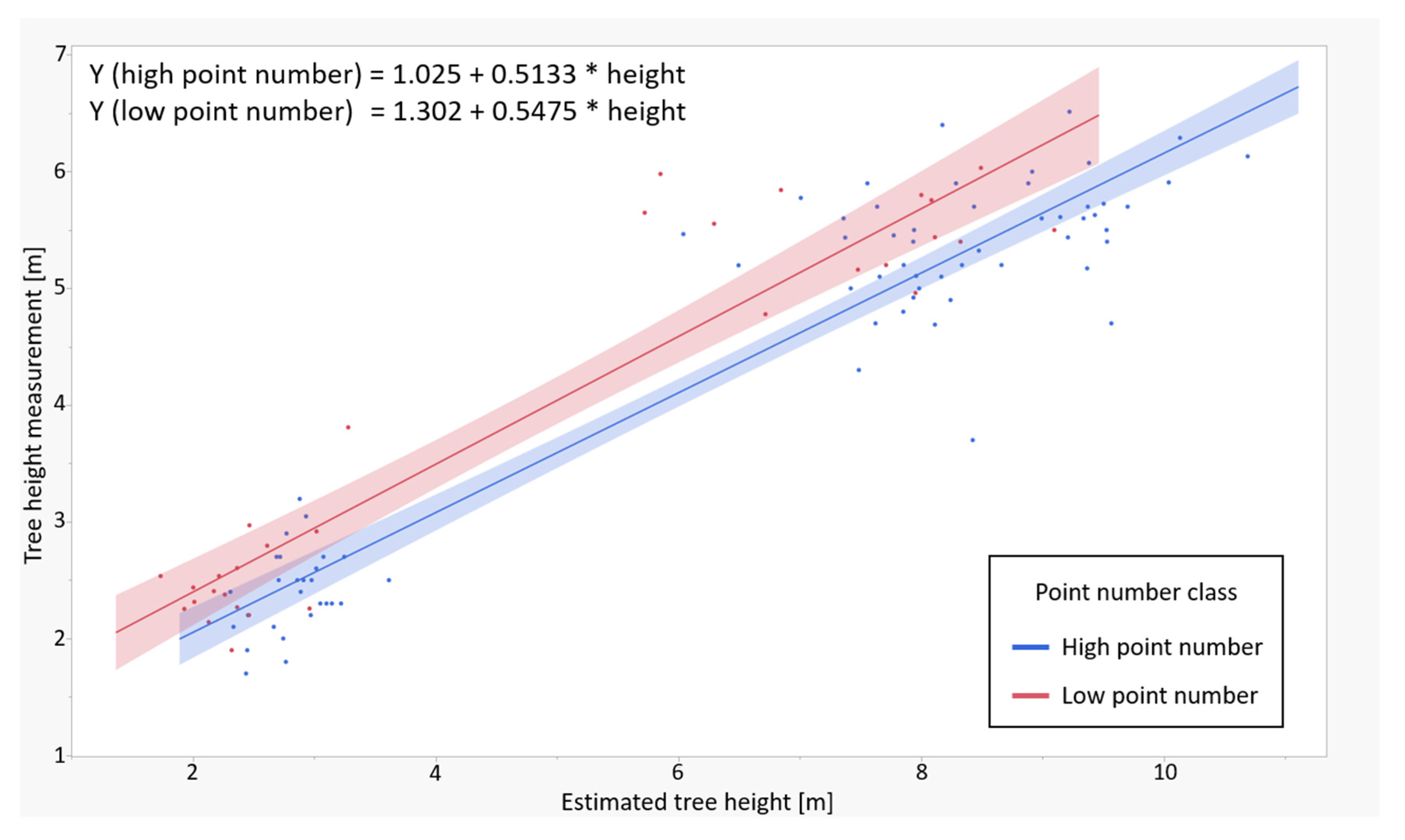
Tree height was delineated on a tree-by-tree basis for each site and year. As shown in the scatter plot in Figure 4, the model’s approximation revealed strong deviations in the number of points within the tree point clusters. To address this, the model was divided into two groups after clustering the point number data according to Ward, and models were fitted individually. This approach was subsequently applied to all other parameters, except for spectral indices, which were not dependent on the number of points. The model’s results are summarized in Table 2.
The height models show intercept values of 1.025 m with a 95% confidence interval of the parameter ranging from 0.73 m to 1.31 m and 1.302 m with a 95% confidence interval ranging from 0.89 m to 1.70 m for trees represented by a high and low number of points, respectively. The model coefficient estimates of 0.5133 and 0.5475 show similar values for both models, with confidence intervals ranging from 0.47 to 0.55 and 0.47 to 0.62 for trees represented by a high and low number of points in the model, respectively. All confidence interval ranges indicate significant parameter estimates with wider ranges for the low-point-number model, leading to less accurate estimations. One reason for that is the lower number of data points in the group of trees represented by a lower number of points: 30 compared to 75 reference data points for the other group. Residues of the model are approximately normally distributed with a mean value close to zero. The model shows limited robustness against outliers, which appeared in the tails of the QQ plot.
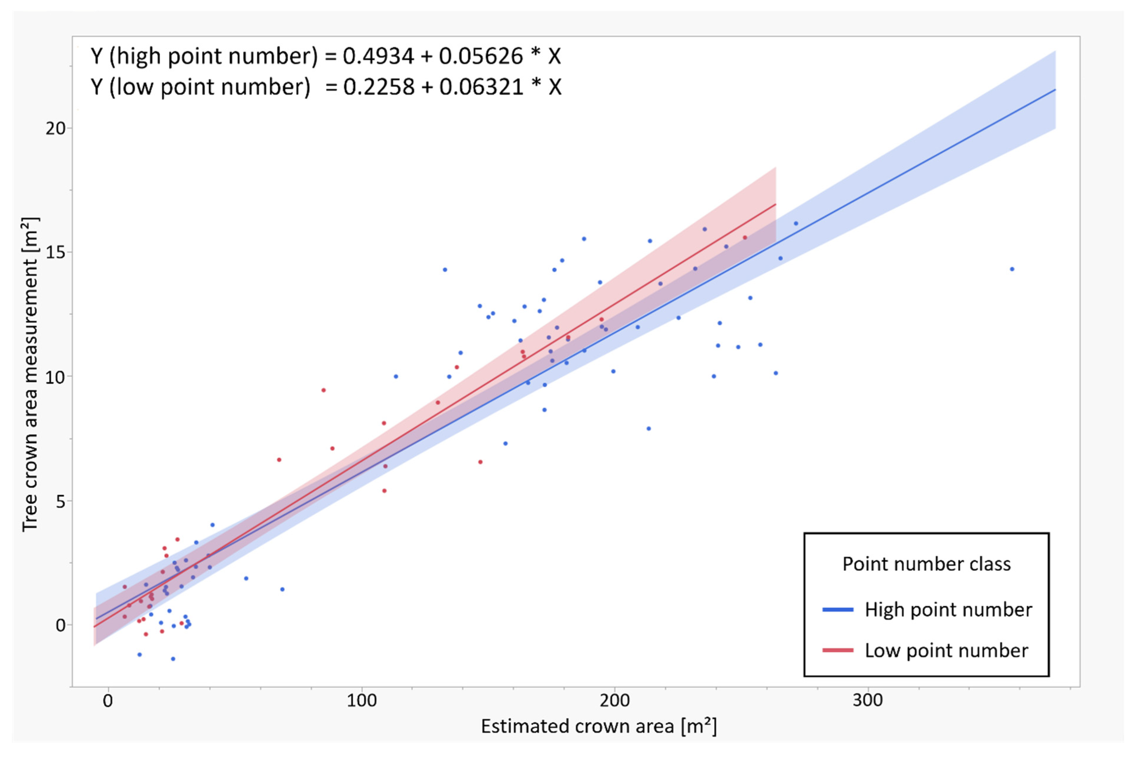
The two sites are clearly separated, forming two-point clusters in Figure 4, because of a general difference in tree height between the two sites. Since trees were taller with larger canopies in Jammel, as mentioned before, the estimations show greater variability for the tree height and projected crown area estimated for the Jammel site. Overall, the model estimations, including both sites for tree height, show R2 values of 0.89 and 0.88, with RMSE values of 0.52 m and 0.54 m for trees with high and low numbers of points, respectively. The models of the projected crown area presented in Figure 5 yielded R2 values of 0.82 and 0.91, along with RMSE values of 2.40 m2 and 1.38 m2, corresponding to trees with high and low numbers of points, respectively. Model intercepts show no significance for both models with respect to the confidence intervals, with values ranging from −0.51 m2 to 1.49 m2 and from −0.48 m2 to 0.99 m2 for trees represented by a high and low number of points, respectively, including the number zero. Both models showed similar, significant parameter estimators for projected crown areas of 0.056—with a confidence interval ranging from 0.050 to 0.062—and 0.063—with a confidence interval ranging from 0.055 to 0.071—for the high- and low-point-number models, respectively. Residues show an approximately normally distributed behavior. Model fitting was performed after applying a Box-Cox transformation to the delineated projected crown area over ground to improve the distribution of model residuals. The estimated values were then back-transformed using λ = 0.314 and λ = 0.686 for trees with a high or low number of points.
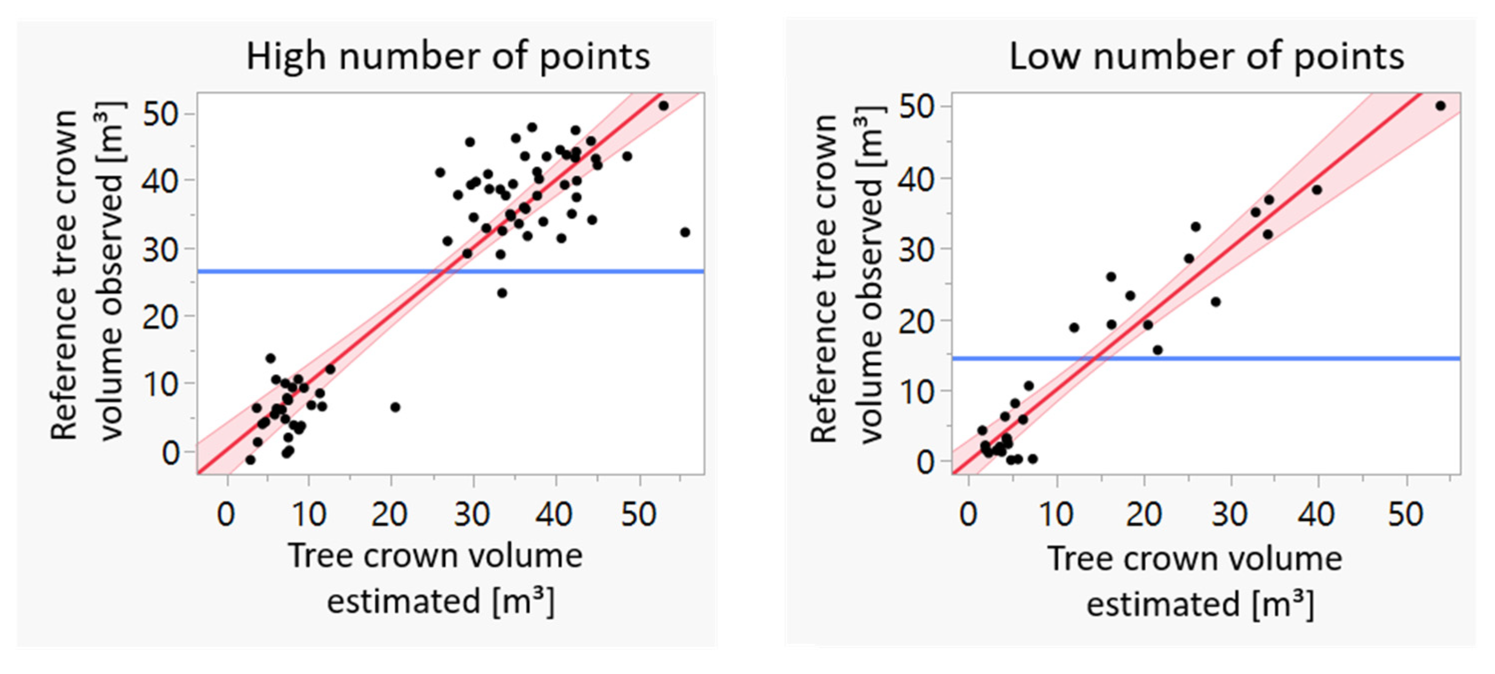
The crown volume per tree was estimated using linear regression models with two parameters, consisting of crown volume and raster cell count, as well as the interaction of these parameters. The model was calibrated separately for trees with high and low numbers of points using the reference measurements. An overview of the parameters and their influence on the model is provided in Table 3. Moreover, the parameter of the tree’s projected crown area was tested in the model but was rejected due to high multicollinearity with the crown volume.
Tree crown volume models, as shown in Figure 6, showed corrected R2 values of 0.85 and 0.91, with RMSE values of 6.48 m3 and 4.26 m3 for trees with high and low numbers of points, respectively, after applying Box-Cox transformation with λ = 0.648 and λ = 0.209. For both point number groups, the same variables were found to have a significant influence on crown volume per tree, namely the estimated volume from the point cloud and the intercept. The intercept has a stronger influence on the model for trees represented by a high number of points compared to the model with a low number of points. Moreover, the interaction multiplier between the variables ‘Raster’ and ‘Volume’ shows a significant negative proportional relationship between the variable effects. This indicates that the influence of the variable ‘Raster’ decreases as the estimated variable ‘Volume’ increases and vice versa. The interaction term has a stronger influence on trees represented by a low number of points, while at the same time, its estimation is more inaccurate, which is given by the wider confidence interval range compared to the model with a high number of points. This could be attributed to the smaller sample size of 30 data points compared to 75. Model residues were approximately normally distributed but showed a weakness for estimating extreme points. To assess the prediction error of both models, an LOOCV was conducted, showing median RMSE values of 4.59 m3 (18.9%) and 3.89 m3 (22.0%), for trees with low and high point numbers, respectively.
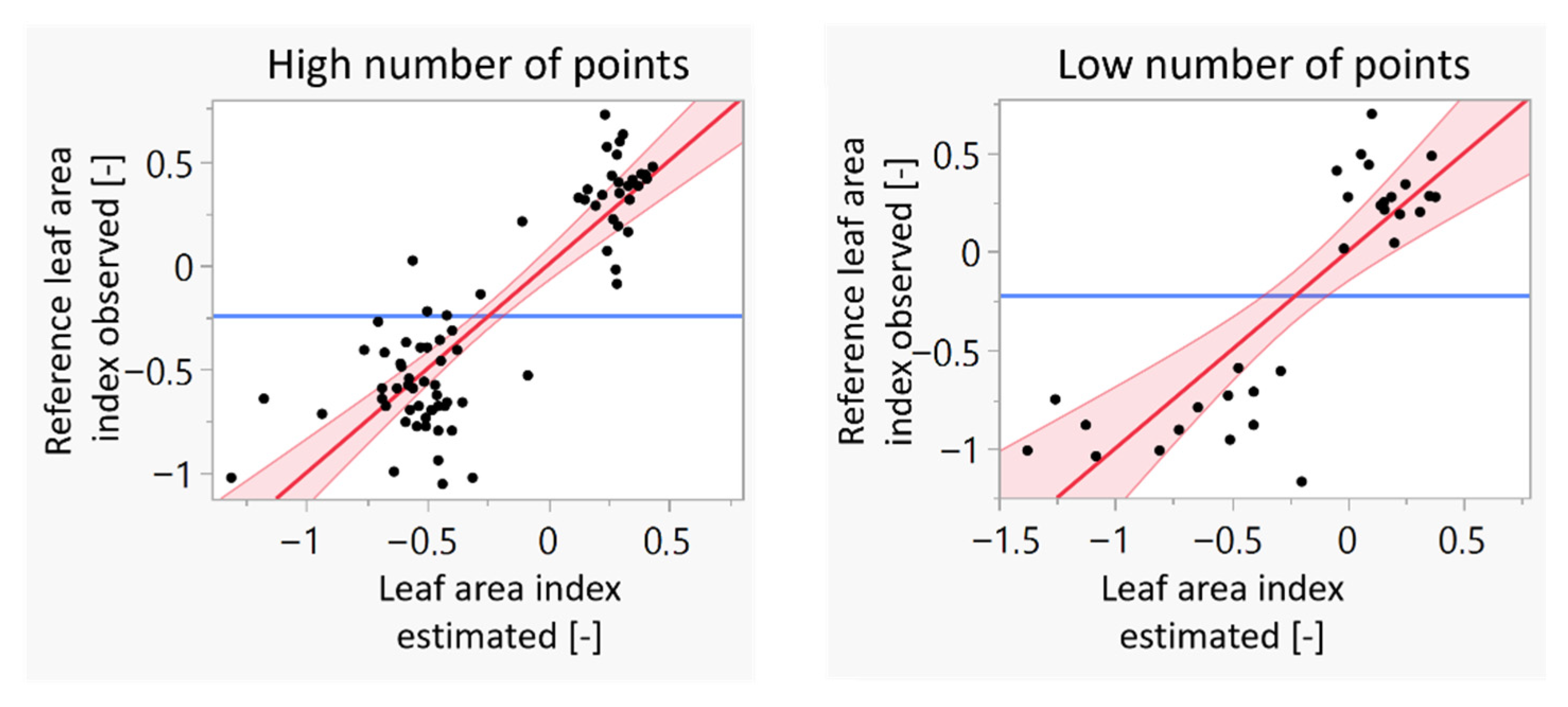
To approximate the LAI per tree from the 3D point cloud, the same delineated parameters used in the tree crown volume models were included in the LAI models. The corresponding models are shown in Figure 7, with R2 of 0.73 or 0.68, RMSE of 0.26 or 0.35, and Box-Cox transformation of λ = 0.03 and λ = 0.055 for trees with high or low numbers of points, respectively.
As shown in Table 4, significant parameters for estimating the trees’ LAIs include the crown volume and the interaction between the raster cell count and the estimated volume of the tree crown. The coefficient of the interaction term indicates a proportional relationship, demonstrating that the influence of the raster cell count increases with greater crown volume and vice versa. This relationship was found to be consistent across both point density groups. The interaction and the parameter volume show a stronger influence in the model for trees represented by a low number of points compared to the model with a high number of points. However, as shown by the wider confidence intervals, the parameter estimators for both terms are less accurate. Model residues were approximately normally distributed with a weakness for estimating extreme points. To assess the model’s prediction error, an LOOCV was conducted, showing a median of 0.16 (17.6%) and 0.20 (21.5%) for the RMSE values for trees with high and low numbers of points, respectively.
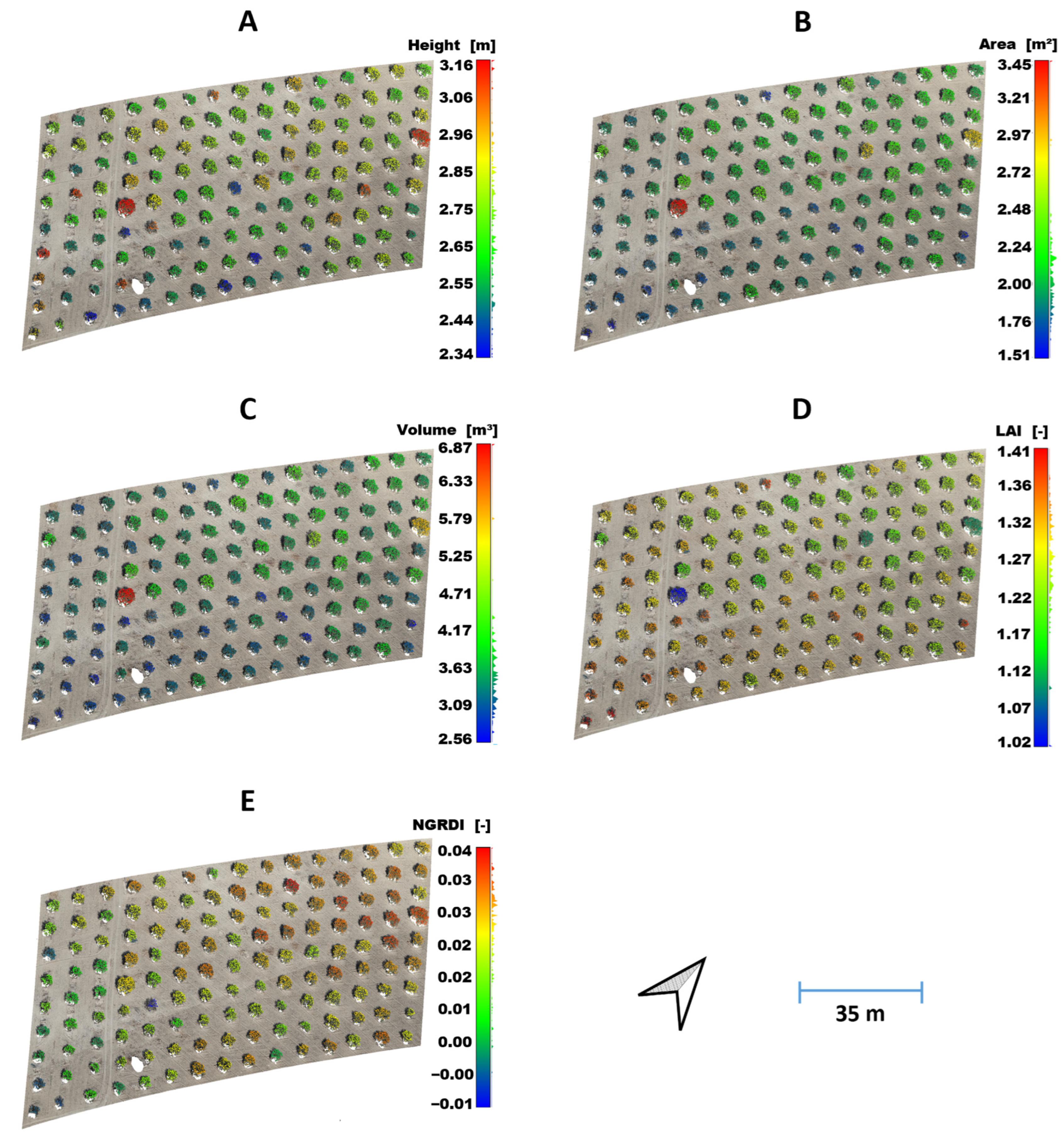
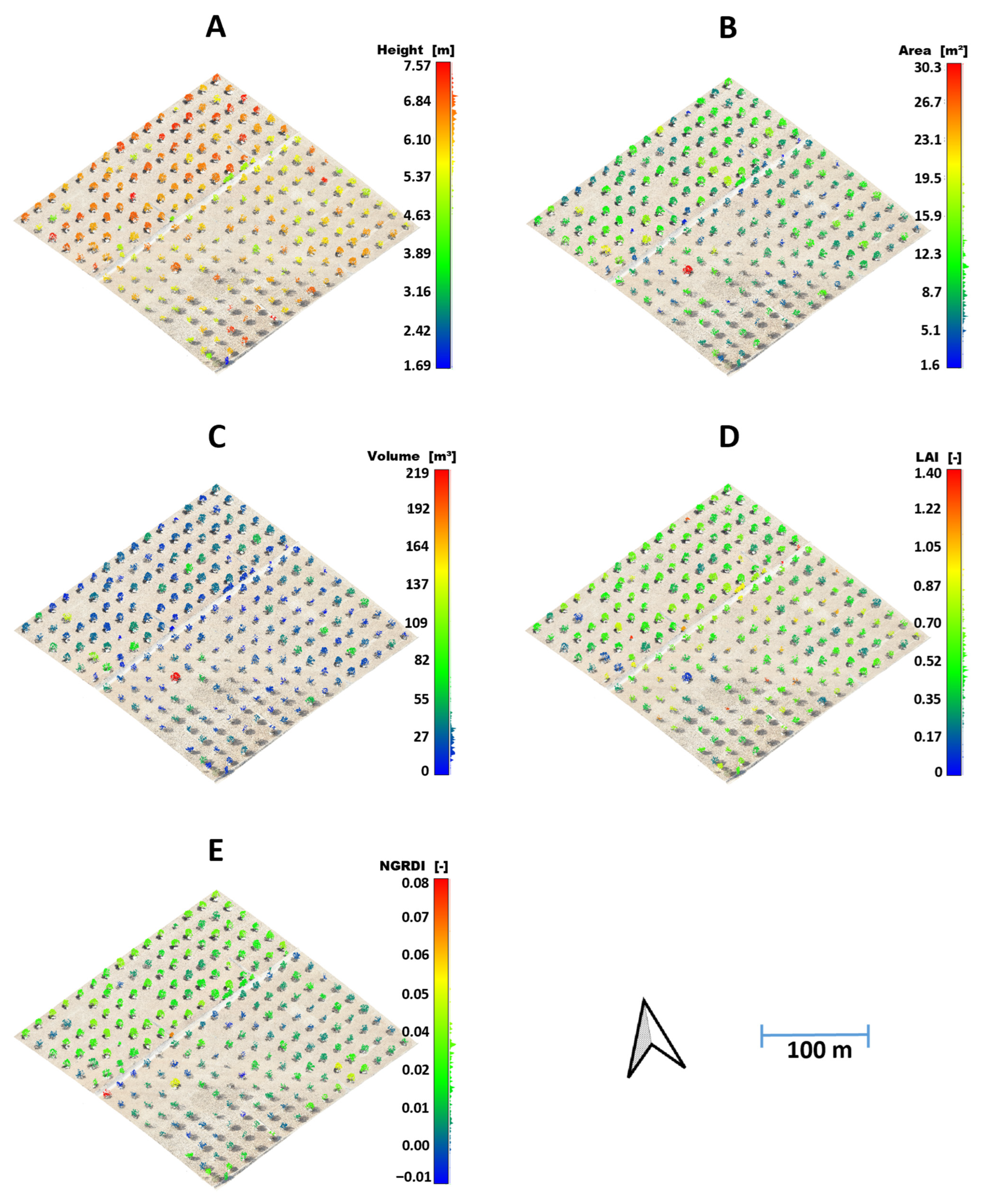
A model delineation for the reference SPAD measurements was not possible, even when multiple statistical parameters of RGB-based indices, namely NGRDI and GLI, were implemented. The best model approximation used the 0.25 quantile and the mean value of the NGRDI, as well as the mean value and the 0.75 quantile of the GLI, but this was only possible with a corrected R2 of 0.34. Since only slightly more than one-third of the SPAD variance can be explained by the model, it is not considered suitable for predicting this value. However, one of the parameters for this model, the NGRDI per tree crown, has already been shown to be useful for counting plants in papaya orchards [64]. Based on the tree parameter models, spatial maps were generated for both orchards. These maps were calibrated with ground-based reference values to represent key variables, including tree height, projected crown area, crown volume, mean LAI per tree, and mean NGRDI, for each study year. Representative maps for Jammel (2022) and Toukaber (2023) are shown in Figure 8 and Figure 9, respectively. The estimated maps provide insights into the spatial distribution of tree status. Each tree is represented as a cluster of 3D points delineated by photogrammetry, with the parameter of interest superimposed as a color gradient. For the Jammel orchard, the mapped tree height shows generally higher values in the northern and northwestern parts, with heights reaching up to 7.5 m, while smaller trees dominate in the eastern corner, as shown in Figure 8A. In the southernmost corner, an extreme value occurred due to photogrammetry, where a tree was poorly separated from surrounding bushes. This tree was excluded from the depiction, and its faulty tree points excluded are colorized in grey. However, the remaining bush points still exhibit extreme height values. For the tree-wise projected crown area, the most expansive tree is in the southeastern part of the orchard, with an area over ground exceeding 30.3 m2, as shown in Figure 8B. Most trees with larger projected crown areas are located in the northwestern part of the field, while trees in the southeastern part exhibit smaller crown areas. The crown volume per tree shows a similar distribution to the tree-wise projected crown area, as shown in Figure 8C. However, the color coding of the map is also influenced by an extreme value from the faulty tree.
The LAI map, Figure 8D, shows values up to 1.41. Interestingly, higher LAI values were estimated for smaller trees in the Jammel orchard, whereas lower LAI values were estimated for larger trees, primarily in the western part of the orchard. This suggests that leaves that are concentrated around more dense branches in smaller trees increase the LAI value. The spectral information from the RGB images is represented as NGRDI values across the orchard, ranging up to 0.08, as shown in Figure 8E. In general, trees in the southeastern part of the orchard exhibited lower NGRDI values, while the northwestern part performed better. However, the highest values were found in the center and southern parts of the orchard.
For the Toukaber orchard, the estimated tree height distribution exhibited lower values compared to the Jammel orchard, as shown in Figure 9A. This can be attributed to the olive variety ‘Chetoui’, which is well adapted to the upland climate of the Beja region and has a more bush-like appearance. Tree heights ranged from 2.34 m to 3.16 m across the orchard. In the central southern area, trees appeared shorter, while taller trees were observed in the northeastern area. The mapped projected crown area also showed higher values in the northeastern part of the orchard, with the rest of the orchard exhibiting relatively low projected crown areas, except for a small area next to the path running through the orchard, as shown in Figure 9B. The distribution of crown volume followed a similar pattern compared to the projected crown area, with a slight increase in values toward the northeastern corner and a maximum near the path. Crown volume values range from 2.56 m3 to 6.87 m3, as shown in Figure 9C.
LAI values ranged from 1.02 to 1.41 in the Toukaber orchard, as shown in Figure 9D. A gradient was observed, with decreasing LAI values from the southwestern to the northeastern part of the orchard. As in Jammel, higher LAI values were associated with smaller trees. This suggests that olive trees do not scale their leaf area proportionally with increases in canopy spread over the ground. Our findings indicate that LAI values decrease as olive trees grow larger. The NGRDI values span a narrow range from zero to 0.04, as shown in Figure 9E. These values are smaller than for trees in Jammel. Within the orchard, the spectral index showed higher values in the northwestern area of the orchard compared to the southeastern area, forming a gradient across the orchard. This gradient appeared to be negatively proportional to the LAI by visual assessment; however, a significant correlation could not be verified.

4. Discussion

In this study, two olive orchards in Tunisia were mapped over two consecutive seasons using low-budget UAV-based RGB sensor technology. From the UAV imagery, three-dimensional point clouds were created using structure-from-motion photogrammetry and automatically analyzed to calculate the target parameters: tree height, projected crown area, crown volume, LAI, and mean NGRDI. The latter parameter was intended for estimating SPAD values, which serve as relative indicators of leaf chlorophyll and nitrogen content.
Structural parameters were automatically estimated from the 3D dense point cloud. Identified olive trees were grouped into classes of trees with a high and low number of points represented in the point cloud. Tree height was estimated from the 95th percentile of the distances from each tree point to the digital terrain model. Linear regression models validated against reference values for tree height yielded R2 values of 0.89 and 0.88, with RMSE values of 0.52 m (relative root mean square error (rRMSE) = 12.1%) and 0.54 m (rRMSE = 14.0%) for high and low numbers of points, respectively. These results are comparable to findings from other studies. Torres-Sanchez et al. [26] estimated olive tree heights in Spain from 50 m altitude UAV flights with RGB-based structure-from-motion photogrammetry. They found a dependency of estimation quality on image overlap, with an error range of -5.85% to 10.1% for a 90% overlap, comparable to the overlap used in this study. Vacca and Vecchi [65] estimated tree heights in an Italian olive orchard from UAV flights at 30 m altitude with 80% forward and 70% sideways overlap, achieving mean absolute errors (MAEs) ranging from 14 cm to 34 cm. Carusso et al. [66] reported an R2 value of 0.79 with a 0.12 m RMSE using high-resolution RGB and multispectral imagery. For other tree crops, Pourreza et al. [67] achieved reliable tree height estimations with rRMSE < 11% in an Iranian cypress plantation, with lower flight altitudes reducing error values. In a Spanish orange tree orchard, Estornell et al. [68] reported an RMSE of 0.26 m for tree height estimations from a 124 m altitude flight with 80% forward and 60% sideways overlap. In a Chinese mango plantation, Bing et al. [69] estimated tree heights from a 30 m altitude oblique perspective with an rRMSE of 5.63% and an R2 of 0.93. The tree height estimation in this study demonstrated reliable results with good coefficients of determination. However, the error values were higher than in comparable studies, despite the favorable flight altitude and image overlap ratio. This lower accuracy is attributed to the open canopy structure of the olive trees at the test sites, which allowed the ground surface to be visible beneath the tree crowns, introducing noise into the photogrammetric process. This issue could be mitigated using a higher-quality camera, but such an approach would conflict with the low-cost objective of this study. Moreover, the use of the 95th percentile for height estimation, which is not common in other studies, may have contributed to the increased error. However, this approach is expected to provide more stable estimation in the presence of noise caused by canopy gaps, albeit with slightly higher errors.
The projected crown area was estimated with R2 values of 0.82 and 0.91 and RMSE values of 2.40 m2 (rRMSE = 28.5%) and 1.38 m2 (rRMSE = 22.7%) for trees with high and low numbers of points, respectively. Model approximations were enhanced in their residual distribution with a Box-Cox transformation of the delineated projected crown area. Carusso et al. [66] found a good correlation (R2 = 0.78) in an Italian olive orchard for the projected crown area between field measurements and orthorectified two-dimensional multispectral NDVI projections. This approach led to smaller RMSE values of 0.44 m2, which shows the benefit of using a multispectral sensor to estimate the projected crown area. Similarly, Catania et al. [29] achieved an R2 = 0.98 and RMSE of 0.54 m using multispectral data. Bing et al. [69] reported a strong correlation of R2 = 0.97 with an rRMSE of 1.0% per tree row using RGB and LiDAR data in a mango orchard. These studies highlight the benefits of incorporating additional sensor information, such as multispectral or LIDAR data, for more accurate results in projected crown area estimations. Also, datasets from the perspective of airborne LiDAR can only be used for structural tree parameter estimations. Cantón-Martínez et al. [70] used airborne LiDAR from 45 m altitude flights to estimate parameters on hedgerow olive trees in southern Spain. The results show comparable or slightly weaker results than presented here: coefficients of determination of 0.72–0.83 for tree height, 0.48–0.64 for projected canopy, and 0.66-0.86 for tree crown volume. Anschaun et al. [71] found LiDAR as a more reliable tool for dense point cloud generation compared to structure from motion in eucalyptus forest tree height estimation. However, the use of LiDAR sensors in general comes with increased costs for the farmers, which leads to stronger adoption barriers.
For olive tree crown volume estimation from UAV imagery, our final Box-Cox transformed regression models achieved R2 values of 0.85 and 0.91 for trees with high and low numbers of points, respectively. For the model’s validation, the LOOCV achieved median RMSE values of 4.59 m3 (18.9%) and 3.89 m3 (22.0%) for trees with low and high point numbers, respectively. In comparison, Caruso et al. [72] reported R2 values of 0.85 to 0.86 for olive tree crown volume estimations using a multiple cylinder model from UAV flights at 50 m altitude. In another study, Carusso et al. [66] achieved an R2 value of 0.82 for olive tree crown volume with an RMSE value of 0.68 m3. The slightly stronger correlation in our convex hull-based approximation is likely due to the inclusion of raster cell counts as an additional parameter, which provides valuable information about branch distributions and inner canopy gaps. However, the multispectral-based methods presented by Caruso et al. [66] and Catania et al. [29] achieved lower RMSE values.
Calibrated LAI regression models in this study, based on volume and raster cell count, achieved R2 values of 0.73 and 0.68, with a median prediction error from LOOCV of 0.16 (17.6%) and 0.20 (21.5%) for the RMSE values of trees with high and low numbers of points, respectively. Caruso et al. [33] indirectly correlated LAI only with the crown volume by linear regression and found a stronger relationship compared to our findings. They studied olive tree varieties ‘Fratonio’ and ‘Leccino’, which were situated in a closed tree row setting. Model estimations for LAI achieved R2 values of 0.84 and 0.88 for ‘Fratonio’ and ‘Leccino’ varieties, respectively. In addition, Caruso et al. [33] and Berni et al. [73] found good model estimations with R2 of over 0.75 when linking multispectral data to LAI.
For leaf chlorophyll estimation, our model showed insufficient correlation and was therefore not considered suitable for the prediction of this parameter. This can be explained by the fact that RGB cameras use wide spectral bands for each color channel that capture a mixed signal from the canopy, as well as bright ground reflections and the lack of information in the NIR and red-edge spectral range. Previous studies have demonstrated the potential of RGB-based indices for nitrogen status estimations in crops such as wheat [39] and in forests [38]. Hunt et al. [74] linked the RGB-based NGRDI value to relative chlorophyll content in grasslands, while Hunt et al. [75] found it sensitive to LAI in crops like alfalfa, corn, and soybean. However, studies suggest that the inclusion of the red-edge and near-infrared range improves model quality and can establish a stable link between chlorophyll contents and reflectance signals. For instance, Noguera et al. [76] used multispectral data and artificial neural networks to estimate nitrogen, potassium, and phosphorus in olive groves, achieving R2 values of 0.63, 0.93, and 0.89, respectively. Similarly, Caruso et al. [72] linked NDVI to leaf chlorophyll content using UAV-based multispectral data. Also, Zhuang et al. [77] used multispectral data to delineate spectral reflectance, vegetation indices, and texture characteristics over an olive orchard in China. In a combined model with multiple parameters, coefficients of determination of up to 0.78 were achieved. In particular, the TCARI/OSAVI spectral index based on multispectral data was beneficial for the model. While multispectral data could improve our models, it would conflict with the low-cost approach we were aiming for in this study. The use of low-cost UAV technology offers high potential for smallholder farms and regions with limited resources. However, financial and technical barriers need to be addressed.

5. Conclusions

In this study, a cost-effective and rapid approach for estimating tree-specific plant parameters in different regions was developed to foster smart farming applications in Tunisian olive orchards. Two olive orchards located in two agroecological zones were mapped using low-cost UAV-based RGB imagery. This locally uncommon approach establishes a foundation for precise monitoring and provides data for future smart farming technologies under use-case conditions. The targeted olive tree parameters included tree height, projected crown area, crown volume, and LAI. In addition, the potential to predict leaf chlorophyll and leaf nitrogen content through indirect SPAD value estimation was tested.
The results demonstrated that all structural target variables could be automatically delineated from three-dimensional RGB point clouds. Individual tree height, projected crown area, and crown volume were mapped for entire olive orchards, along with tree-specific LAI values. The approach was applied successfully in both orchards, covering highly different olive tree varieties and environmental conditions and demonstrating the adaptability of the algorithm. It was also shown that the number of points per tree influenced the accuracy of structural tree parameter estimations. However, due to the low-cost approach, error ratios of all target values were slightly higher compared to studies using additional sensor information or higher-resolution data. Moreover, the SPAD value could not be reliably estimated from the spectral indices NGRDI and GLI, and this model was therefore not considered suitable for the prediction of this parameter.
The estimated maps of tree parameters provided valuable insights into the spatial distribution of successfully delineated values in a three-dimensional form. All necessary calculations were done in less than 16 h per field and are therefore capable of delivering tree parameter insights in a reasonable amount of time. The calculated maps provide a comprehensive overview of the distribution of key structural parameters and can therefore play a key role in farm management under resource constraints. However, the approach was unable to produce viable results for delineating a similar model for leaf nitrogen and leaf chlorophyll content from the RGB data. To address this limitation, we propose additional research using adapted camera sensors, particularly multispectral sensors with bands sensitive to the red edge. Also, the application of modified low-cost NIR cameras or the use of machine learning algorithms, taking features like texture or 3D metrics into account, could be possible ways forward for upcoming field studies in Tunisia. Moreover, it is suggested to repeat similar field trials from this study using the tested approach on additional olive groves in Tunisia in order to ensure broad applicability for local varieties. Despite these limitations, due to the high level of automation in the proposed approach and the ease of use of UAV technology, the provided results are a step toward enabling smart olive farming in Tunisia.

Author Contributions

Conceptualization, O.B., P.E., A.B.H. and M.H.; data curation, O.B., A.G., A.B.H. and M.H.; formal analysis, O.B., A.G., A.B.H. and M.H.; funding acquisition, O.B. and M.S.; investigation O.B., P.E., A.B.H. and M.H.; methodology, O.B., A.G., A.B.H. and M.H.; project administration, O.B. and M.S.; visualization M.H.; writing—original draft, O.B. and M.H.; writing—review and editing, P.E., A.G., A.B.H., M.S. and C.W. All authors have read and agreed to the published version of the manuscript.

Funding

This article was co-funded by the European Union Horizon 2020 Research and Innovation Programme under grant agreement No. 861924.

Data Availability Statement

The datasets generated and/or analyzed during the current study are available from the corresponding author on reasonable request.

Acknowledgments

We want to thank Hanen Kefi for her contributions in planning, conducting, and analyzing multiple field campaigns in Jammel and Toukaber.

Conflicts of Interest

The authors declare no conflicts of interest. We have adhered to the journal’s policy on originality and confirm that the content of this manuscript is not under consideration by any other publication.

References

  1. Gargouri, K.; Mhiri, A. Relationship between soil fertility, phosphorus and potassium nutrition of the olive in Tunisia. Opt. Mediterr. 2003, 50, 199–204. [Google Scholar]
  2. Nieto, O.M.; Castro, J.; Fernández, E.; Smith, P. Simulation of soil organic carbon stocks in a Mediterranean olive grove under different soil-management systems using the RothC model. Soil Use Manag. 2010, 26, 118–125. [Google Scholar] [CrossRef] [Scilit]
  3. Chehab, H.; Tekayab, M.; Ouhibic, M.; Gouiaad, M.; Zakhamae, H.; Mahjouba, Z.; Laamaria, S.; Sfinaa, H.; Chihaouia, B.; Boujnaha, D.; et al. Effects of compost, olive mill wastewater and legume cover crops on soil characteristics, tree performance and oil quality of olive trees cv. Chemlali grown under organic farming system. Sci. Hortic. 2019, 253, 163–171. [Google Scholar] [CrossRef] [Scilit]
  4. Addesso, R.; Araniti, F.; Bloise, A.; Mininni, A.N.; Dichio, B.; López-González, D.; Elshafie, E.S.; Ellerbrock, R.H.; Ellerbrock, L.S.; Filser, J.; et al. Soil organic matter quality in an olive orchard differently managed for 21 years: Insights into its distribution through soil aggregates and depth. Agric. Ecosyst. Environ. 2025, 380, 109388. [Google Scholar] [CrossRef] [Scilit]
  5. Aguilera, E.; Lassaletta, L.; Gattinger, A.; Gimeno, B.S. Managing soil carbon for climate change mitigation and adaptation in Mediterranean cropping systems: A meta-analysis. Agric. Ecosyst. Environ. 2013, 168, 25–36. [Google Scholar] [CrossRef] [Scilit]
  6. Freyer, B.; Ellssel, P.; Friedel, J.K.; Möller, K. The contribution of organic farming systems to soil fertility—A systems perspective. In Encyclopedia of Soils in the Environment, 2nd ed.; Elsevier: Amsterdam, The Netherlands, 2023; Volume 3. [Google Scholar] [CrossRef] [Scilit]
  7. Ruiz-Cátedra, G.; Calero, J.; Domouso, P.; García-Ruiz, R. Do management practices which enhance nature-based processes improve soil health in olive groves? Geoderma 2025, 457, 117276. [Google Scholar] [CrossRef] [Scilit]
  8. Zevgolis, Y.G.; Kouris, A.; Christopoulos, A.; Dimitrakopoulos, P.G. Linking Thermal Indices, Productivity, Phenotypic Traits, and Stressors for Assessing the Health of Centennial Traditional Olive Trees. Appl. Sci. 2023, 13, 11443. [Google Scholar] [CrossRef] [Scilit]
  9. Guermazi, E.; Wali, A.; Ksibi, M. Combining remote sensing, SPAD readings, and laboratory analysis for monitoring olive groves and olive oil quality. Precis. Agric. 2024, 25, 65–82. [Google Scholar] [CrossRef] [Scilit]
  10. Roma, E.; Catania, P. Precision Oliviculture: Research Topics, Challenges, and Opportunities—A Review. Remote Sens. 2022, 14, 1668. [Google Scholar] [CrossRef] [Scilit]
  11. Ampatzidis, Y.; Costa, L.; Albrecht, U. Precision nutrient management utilizing UAV multispectral imaging and artificial intelligence. In Proceedings of the XXXI International Horticultural Congress (IHC2022): III International Symposium on Mechanization, Precision Horticulture, and Robotics: Precision and Digital Horticulture in Field Environments; ISHS: Rosemead, CA, USA, 2022; Volume 1360, pp. 321–330. [Google Scholar]
  12. Colovic, M.; Stellacci, A.M.; Mzid, N.; Di Venosa, M.; Todorovic, M.; Cantore, V.; Albrizio, R. Comparative Performance of Aerial RGB vs. Ground Hyperspectral Indices for Evaluating Water and Nitrogen Status in Sweet Maize. Agronomy 2024, 14, 562. [Google Scholar] [CrossRef] [Scilit]
  13. Sola-Guirado, R.; Castillo-Ruiz, F.; Jiménez-Jiménez, F.; Blanco-Roldan, G.; Castro-Garcia, S.; Gil-Ribes, J. Olive Actual “on Year” Yield Forecast Tool Based on the Tree Canopy Geometry Using UAS Imagery. Sensors 2017, 17, 1743. [Google Scholar] [CrossRef] [Scilit] [PubMed]
  14. Yang, R.; Liu, L.; Liu, Q.; Li, X.; Yin, L.; Hao, X.; Ma, Y.; Song, Q. Validation of leaf area index measurement system based on wireless sensor network. Sci. Rep. 2022, 12, 4668. [Google Scholar] [CrossRef] [Scilit] [PubMed]
  15. Haberman, A.; Dag, A.; Shtern, N.; Zipori, I.; Erel, R.; Ben-Gal, A.; Yermiyahu, U. Significance of proper nitrogen fertilization for olive productivity in intensive cultivation. Sci. Hortic. 2019, 246, 710–717. [Google Scholar] [CrossRef] [Scilit]
  16. Sánchez-Fernández, L.; Barrera, M.; Martínez-Guanter, J.; Pérez-Ruiz, M. Drift reduction in orchards through the use of an autonomous UAV system. Comput. Electron. Agric. 2023, 211, 107981. [Google Scholar] [CrossRef] [Scilit]
  17. Abdelmoula, H.; Kallel, A.; Roujean, J.-L.; Gastellu-Etchegorry, J.-P. Dynamic Retrieval of Olive Tree Properties Using Bayesian Model and Sentinel-2 Images. IEEE J. Sel. Top. Appl. Earth Obs. Remote Sens. 2021, 14, 9267–9286. [Google Scholar] [CrossRef] [Scilit]
  18. Sanz, R.; Llorens, J.; Escolà, A.; Arnó, J.; Planas, S.; Román, C.; Rosell-Polo, J.R. LIDAR and non-LIDAR-based canopy parameters to estimate the leaf area in fruit trees and vineyard. Agric. For. Meteorol. 2018, 260–261, 229–239. [Google Scholar] [CrossRef] [Scilit]
  19. Knerl, A.; Anthony, B.; Serra, S.; Musacchi, S. Optimization of Leaf Area Estimation in a High-Density Apple Orchard Using Hemispherical Photography. Horts 2018, 53, 799–804. [Google Scholar] [CrossRef] [Scilit]
  20. Boussadia, O.; Steppe, K.; Zgallai, H.; Ben El Hadj, S.; Braham, M.; Lemeur, R.; Van Labeke, M.C. Effects of nitrogen deficiency on leaf photosynthesis, carbohydrate status and biomass production in two olive cultivars ‘Meski’ and ‘Koroneiki’. Sci. Hortic. 2010, 123, 336–342. [Google Scholar] [CrossRef] [Scilit]
  21. Muñoz-Huerta, R.; Guevara-Gonzalez, R.; Contreras-Medina, L.; Torres-Pacheco, I.; Prado-Olivarez, J.; Ocampo-Velazquez, R. A Review of Methods for Sensing the Nitrogen Status in Plants: Advantages, Disadvantages and Recent Advances. Sensors 2013, 13, 10823–10843. [Google Scholar] [CrossRef] [Scilit]
  22. Boussadia, O.; Steppe, K.; Zgallai, H.; Ben El Hadj, S.; Braham, M.; Lemeur, R.; Van Labeke, M.-C. Nondestructive determination of nitrogen and chlorophyll content in olive tree leaves and the relation with photosynthesis and fluorescence parameters. Photosynthetica 2011, 49, 149–153. [Google Scholar] [CrossRef] [Scilit]
  23. Alexopoulos, A.; Koutras, K.; Ali, S.B.; Puccio, S.; Carella, A.; Ottaviano, R.; Kalogeras, A. Complementary Use of Ground-Based Proximal Sensing and Airborne/Spaceborne Remote Sensing Techniques in Precision Agriculture: A Systematic Review. Agronomy 2023, 13, 1942. [Google Scholar] [CrossRef] [Scilit]
  24. Zhang, C.; Valente, J.; Kooistra, L.; Guo, L.; Wang, W. Orchard management with small unmanned aerial vehicles: A survey of sensing and analysis approaches. Precis. Agric. 2021, 22, 2007–2052. [Google Scholar] [CrossRef] [Scilit]
  25. Smigaj, M.; Gaulton, R. Capturing hedgerow structure and flowering abundance with UAV remote sensing. Remote Sens. Ecol. Conserv. 2021, 7, 521–533. [Google Scholar] [CrossRef] [Scilit]
  26. Torres-Sánchez, J.; López-Granados, F.; Borra-Serrano, I.; Peña, J.M. Assessing UAV-collected image overlap influence on computation time and digital surface model accuracy in olive orchards. Precis. Agric. 2018, 19, 115–133. [Google Scholar] [CrossRef] [Scilit]
  27. Yang, K.; Zhang, H.; Wang, F.; Lai, R. Extraction of Broad-Leaved Tree Crown Based on UAV Visible Images and OBIA-RF Model: A Case Study for Chinese Olive Trees. Remote Sens. 2022, 14, 2469. [Google Scholar] [CrossRef] [Scilit]
  28. Mendes dos Santos, L.; e Silva Ferraz, G.A.; de Souza Barbosa, B.D.; Diotto, A.V.; Andrade, M.T.; Conti, L.; Rossi, G. Determining the Leaf Area Index and Percentage of Area Covered by Coffee Crops Using UAV RGB Images. IEEE J. Sel. Top. Appl. Earth Obs. Remote Sens. 2020, 13, 6401–6409. [Google Scholar] [CrossRef] [Scilit]
  29. Catania, P.; Roma, E.; Orlando, S.; Vallone, M. Evaluation of Multispectral Data Acquired from UAV Platform in Olive Orchard. Horticulturae 2023, 9, 133. [Google Scholar] [CrossRef] [Scilit]
  30. Stateras, D.; Kalivas, D. Assessment of Olive Tree Canopy Characteristics and Yield Forecast Model Using High Resolution UAV Imagery. Agriculture 2020, 10, 385. [Google Scholar] [CrossRef] [Scilit]
  31. Mathews, A.; Jensen, J. Visualizing and Quantifying Vineyard Canopy LAI Using an Unmanned Aerial Vehicle (UAV) Collected High Density Structure from Motion Point Cloud. Remote Sens. 2013, 5, 2164–2183. [Google Scholar] [CrossRef] [Scilit]
  32. Comba, L.; Biglia, A.; Ricauda Aimonino, D.; Tortia, C.; Mania, E.; Guidoni, S.; Gay, P. Leaf Area Index evaluation in vineyards using 3D point clouds from UAV imagery. Precis. Agric. 2020, 21, 881–896. [Google Scholar] [CrossRef] [Scilit]
  33. Caruso, G.; Palai, G.; Tozzini, L.; Gucci, R. Using Visible and Thermal Images by an Unmanned Aerial Vehicle to Monitor the Plant Water Status, Canopy Growth and Yield of Olive Trees (cvs. Frantoio and Leccino) under Different Irrigation Regimes. Agronomy 2022, 12, 1904. [Google Scholar] [CrossRef] [Scilit]
  34. Li, M.; Shamshiri, R.R.; Schirrmann, M.; Weltzien, C.; Shafian, S.; Laursen, M.S. UAV Oblique Imagery with an Adaptive Micro-Terrain Model for Estimation of Leaf Area Index and Height of Maize Canopy from 3D Point Clouds. Remote Sens. 2022, 14, 585. [Google Scholar] [CrossRef] [Scilit]
  35. Li, F.; Gnyp, M.L.; Jia, L.; Miao, Y.; Yu, Z.; Koppe, W.; Bareth, G.; Chen, X.; Zhang, F. Estimating N status of winter wheat using a handheld spectrometer in the North China Plain. Field Crops Res. 2008, 106, 77–85. [Google Scholar] [CrossRef] [Scilit]
  36. Hunt, E.R.; Doraiswamy, P.C.; McMurtrey, J.E.; Daughtry, C.S.T.; Perry, E.M.; Akhmedov, B. A visible band index for remote sensing leaf chlorophyll content at the canopy scale. Int. J. Appl. Earth Obs. Geoinf. 2013, 21, 103–112. [Google Scholar] [CrossRef] [Scilit]
  37. Liu, Y.; Hatou, K.; Aihara, T.; Kurose, S.; Akiyama, T.; Kohno, Y.; Lu, S.; Omasa, K. A Robust Vegetation Index Based on Different UAV RGB Images to Estimate SPAD Values of Naked Barley Leaves. Remote Sens. 2021, 13, 686. [Google Scholar] [CrossRef] [Scilit]
  38. Valverde, J.C. Estimation of leaf nitrogen content from nondestructive methods in Eucalyptus tereticornis and Eucalyptus saligna plantations. Rev. Fac. Nac. Agron. Medellín 2021, 74, 9655–9666. [Google Scholar] [CrossRef] [Scilit]
  39. Li, H.; Yang, G.; Long, H.; Feng, H.; Xu, B.; Zhao, C. Estimating characteristic coefficient of vertical leaf nitrogen profile within wheat canopy from spectral reflectance. Comput. Electron. Agric. 2023, 206, 107652. [Google Scholar] [CrossRef] [Scilit]
  40. Massaoudi, A.; Berguiga, A.; Harchay, A.; Ben Ayed, M.; Belmabrouk, H. Spectral and Energy Efficiency Trade-Off in UAV-Based Olive Irrigation Systems. Appl. Sci. 2023, 13, 10739. [Google Scholar] [CrossRef] [Scilit]
  41. Ksibi, A.; Ayadi, M.; Soufiene, B.O.; Jamjoom, M.M.; Ullah, Z. MobiRes-Net: A Hybrid Deep Learning Model for Detecting and Classifying Olive Leaf Diseases. Appl. Sci. 2022, 12, 10278. [Google Scholar] [CrossRef] [Scilit]
  42. Hobart, M.; Pflanz, M.; Weltzien, C.; Schirrmann, M. Growth height determination of tree walls for precise monitoring in apple fruit production using UAV photogrammetry. Remote Sens. 2020, 12, 1656. [Google Scholar] [CrossRef] [Scilit]
  43. Perry, S.G.; Fraser, A.B.; Thomson, D.W.; Norman, J.M. Indirect sensing of plant canopy structure with simple radiation measurements. Agric. For. Meteorol. 1988, 42, 255–278. [Google Scholar] [CrossRef] [Scilit]
  44. Campbell, G.; Norman, J. The description and measurement of plant canopy structure. Plant Canopies Their Growth Form Funct. 1989, 1, 19. [Google Scholar]
  45. LI-COR Environmental. LAI-2200C Plant Canopy Analyzer Instruction Manual, 984-14112; LI-COR, Inc.: Lincoln, NE, USA, 2019; Available online: https://licor.app.boxenterprise.net/s/fqjn5mlu8c1a7zir5qel (accessed on 19 April 2026).
  46. LI-COR Environmental. FV2200_21_Guide 2.1; LI-COR, Inc.: Lincoln, NE, USA, 2014; Available online: http://download.opensource.licor.com/projects/fv2200/docs/FV2200_2.1_Guide.pdf (accessed on 19 April 2026).
  47. Kobayashi, H.; Ryu, Y.; Baldocchi, D.D.; Welles, J.M.; Norman, J.M. On the correct estimation of gap fraction: How to remove scattered radiation in gap fraction measurements? Agric. For. Meteorol. 2013, 174–175, 170–183. [Google Scholar] [CrossRef] [Scilit]
  48. Kjeldahl, J. Neue Methode zur Bestimmung des Stickstoffs in organischen Körpern. Z. Für Anal. Chem. 1883, 22, 366–382. [Google Scholar] [CrossRef] [Scilit]
  49. Tinkham, W.T.; Swayze, N.C. Influence of Agisoft Metashape Parameters on UAS Structure from Motion Individual Tree Detection from Canopy Height Models. Forests 2021, 12, 250. [Google Scholar] [CrossRef] [Scilit]
  50. Zhang, W.; Qi, J.; Wan, P.; Wang, H.; Xie, D.; Wang, X.; Yan, G. An Easy-to-Use Airborne LiDAR Data Filtering Method Based on Cloth Simulation. Remote Sens. 2016, 8, 501. [Google Scholar] [CrossRef] [Scilit]
  51. Roussel, J.-R.; Auty, D.; Coops, N.C.; Tompalski, P.; Goodbody, T.R.H.; Meador, A.S.; Bourdon, J.-F.; de Boissieu, F.; Achim, A. lidR: An R package for analysis of Airborne Laser Scanning (ALS) data. Remote Sens. Environ. 2020, 251, 112061. [Google Scholar] [CrossRef] [Scilit]
  52. Roussel, J.-R.; Auty, D. Airborne LiDAR Data Manipulation and Visualization for Forestry Applications. 2024. Available online: https://github.com/r-lidar/lidR (accessed on 19 April 2026).
  53. Cleveland, W.S.; Grosse, E.; Shyu, W.M. Local regression models. In Statistical Models in S; Routledge: Oxfordshire, UK, 2017; pp. 309–376. [Google Scholar]
  54. Popescu, S.C.; Wynne, R.H. Seeing the Trees in the Forest: Using Lidar and Multispectral Data Fusion with Local Filtering and Variable Window Size for Estimating Tree Height. Photogramm. Eng. Remote Sens. 2004, 5, 589–604. [Google Scholar] [CrossRef] [Scilit]
  55. Ester, M.; Kriegel, H.-P.; Sander, J.; Xu, X. A density-based algorithm for discovering clusters in large spatial databases with noise. In Kdd; AAAI: Washington, DC, USA, 1996; pp. 226–231. [Google Scholar]
  56. Hahsler, M.; Piekenbrock, M.; Doran, D. dbscan: Fast Density-Based Clustering with R. J. Stat. Softw. 2019, 91, 1–30. [Google Scholar] [CrossRef] [Scilit]
  57. Hahsler, M.; Piekenbrock, M. dbscan: Density-Based Spatial Clustering of Applications with Noise (DBSCAN) and Related Algorithms. 2023. Available online: https://cran.r-project.org/web/packages/dbscan/index.html (accessed on 19 April 2026).
  58. Barber, C.B.; Dobkin, D.P.; Huhdanpaa, H. The quickhull algorithm for convex hulls. ACM Trans. Math. Softw. 1996, 22, 469–483. [Google Scholar] [CrossRef] [Scilit]
  59. Habel, K.; Grasman, R.; Gramacy, R.B.; Mozharovskyi, P.; Sterratt, D.C. Geometry: Mesh Generation and Surface Tessellation. 2023. Available online: https://cran.r-project.org/web/packages/geometry/index.html (accessed on 19 April 2026).
  60. Box, G.E.; Cox, D.R. An analysis of transformations. J. R. Stat. Soc. Ser. B Stat. Methodol. 1964, 26, 211–243. [Google Scholar] [CrossRef] [Scilit]
  61. Ward, J.H. Hierarchical Grouping to Optimize an Objective Function. J. Am. Stat. Assoc. 1963, 58, 236–244. [Google Scholar] [CrossRef]
  62. R Core Team. R: A Language and Environment for Statistical Computing; R Foundation for Statistical Computing: Vienna, Austria, 2024. [Google Scholar]
  63. Tucker, C.J. Red and photographic infrared linear combinations for monitoring vegetation. Remote Sens. Environ. 1979, 8, 127–150. [Google Scholar] [CrossRef] [Scilit]
  64. Lai, S.; Ming, H.; Huang, Q.; Qin, Z.; Duan, L.; Cheng, F.; Han, G. Remote Sensing Extraction of Crown Planar Area and Plant Number of Papayas Using UAV Images with Very High Spatial Resolution. Agronomy 2024, 14, 636. [Google Scholar] [CrossRef] [Scilit]
  65. Vacca, G.; Vecchi, E. UAV Photogrammetric Surveys for Tree Height Estimation. Drones 2024, 8, 106. [Google Scholar] [CrossRef] [Scilit]
  66. Caruso, G.; Palai, G.; Marra, F.P.; Caruso, T. High-Resolution UAV Imagery for Field Olive (Olea europaea L.) Phenotyping. Horticulturae 2024, 7, 258. [Google Scholar] [CrossRef] [Scilit]
  67. Pourreza, M.; Moradi, F.; Khosravi, M.; Deljouei, A.; Vanderhoof, M.K. GCPs-Free Photogrammetry for Estimating Tree Height and Crown Diameter in Arizona Cypress Plantation Using UAV-Mounted GNSS RTK. Forests 2022, 13, 1905. [Google Scholar] [CrossRef] [Scilit]
  68. Estornell, J.; Martí, J.; Hadas, E.; López-Cortés, I.; Velázquez-Martí, B.; Fernández-Sarría, A. Biomass estimation of abandoned orange trees using UAV-SFM 3D points. Int. J. Appl. Earth Obs. Geoinf. 2024, 130, 103931. [Google Scholar] [CrossRef] [Scilit]
  69. Bing, Q.; Zhang, R.; Zhang, L.; Li, L.; Chen, L. UAV-SfM Photogrammetry for Canopy Characterization Toward Unmanned Aerial Spraying Systems Precision Pesticide Application in an Orchard. Drones 2025, 9, 151. [Google Scholar] [CrossRef] [Scilit]
  70. Cantón-Martínez, S.; Mesas-Carrascosa, F.J.; Rosa, R.D.L.; López-Granados, F.; León, L.; Pérez-Porras, F.; Páez, F.C.; Torres-Sánchez, J. Evaluation of Canopy Growth in Rainfed Olive Hedgerows Using UAV-LiDAR. Horticulturae 2024, 10, 952. [Google Scholar] [CrossRef] [Scilit]
  71. Anschau, M.; Hamilton, G. A Comparison of UAV-Derived Dense Point Clouds Using LiDAR and NIR Photogrammetry in an Australian Eucalypt Forest. Remote Sens. 2023, 15, 1694. [Google Scholar] [CrossRef] [Scilit]
  72. Caruso, G.; Zarco-Tejada, P.J.; González-Dugo, V.; Moriondo, M.; Tozzini, L.; Palai, G.; Rallo, G.; Hornero, A.; Primicerio, J.; Gucci, R. High-resolution imagery acquired from an unmanned platform to estimate biophysical and geometrical parameters of olive trees under different irrigation regimes. PLoS ONE 2019, 14, e0210804. [Google Scholar] [CrossRef] [Scilit]
  73. Berni, J.A.J.; Zarco-Tejada, P.J.; Sepulcre-Cantó, G.; Fereres, E.; Villalobos, F. Mapping canopy conductance and CWSI in olive orchards using high resolution thermal remote sensing imagery. Remote Sens. Environ. 2009, 113, 2380–2388. [Google Scholar] [CrossRef] [Scilit]
  74. Hunt, E.R.; Daughtry, C.S.T.; Eitel, J.U.H.; Long, D.S. Remote Sensing Leaf Chlorophyll Content Using a Visible Band Index. Agron. J. 2011, 103, 1090–1099. [Google Scholar] [CrossRef] [Scilit]
  75. Hunt, E.R.; Cavigelli, M.; Daughtry, C.S.T.; Mcmurtrey, J.E.; Walthall, C.L. Evaluation of Digital Photography from Model Aircraft for Remote Sensing of Crop Biomass and Nitrogen Status. Precis. Agric. 2005, 6, 359–378. [Google Scholar] [CrossRef] [Scilit]
  76. Noguera, M.; Aquino, A.; Ponce, J.M.; Cordeiro, A.; Silvestre, J.; Arias-Calderón, R.; da Encarnação Marcelo, M.; Jordão, P.; Andújar, J.M. Nutritional status assessment of olive crops by means of the analysis and modelling of multispectral images taken with UAVs. Biosyst. Eng. 2021, 211, 1–18. [Google Scholar] [CrossRef] [Scilit]
  77. Zhuang, W.; Li, D.; Kou, W.; Lu, N.; Wu, F.; Sun, S.; Liu, Z. A Multi-Feature Estimation Model for Olive Canopy Chlorophyll Combining XGBoost with UAV Imagery. Agronomy 2025, 15, 2718. [Google Scholar] [CrossRef] [Scilit]
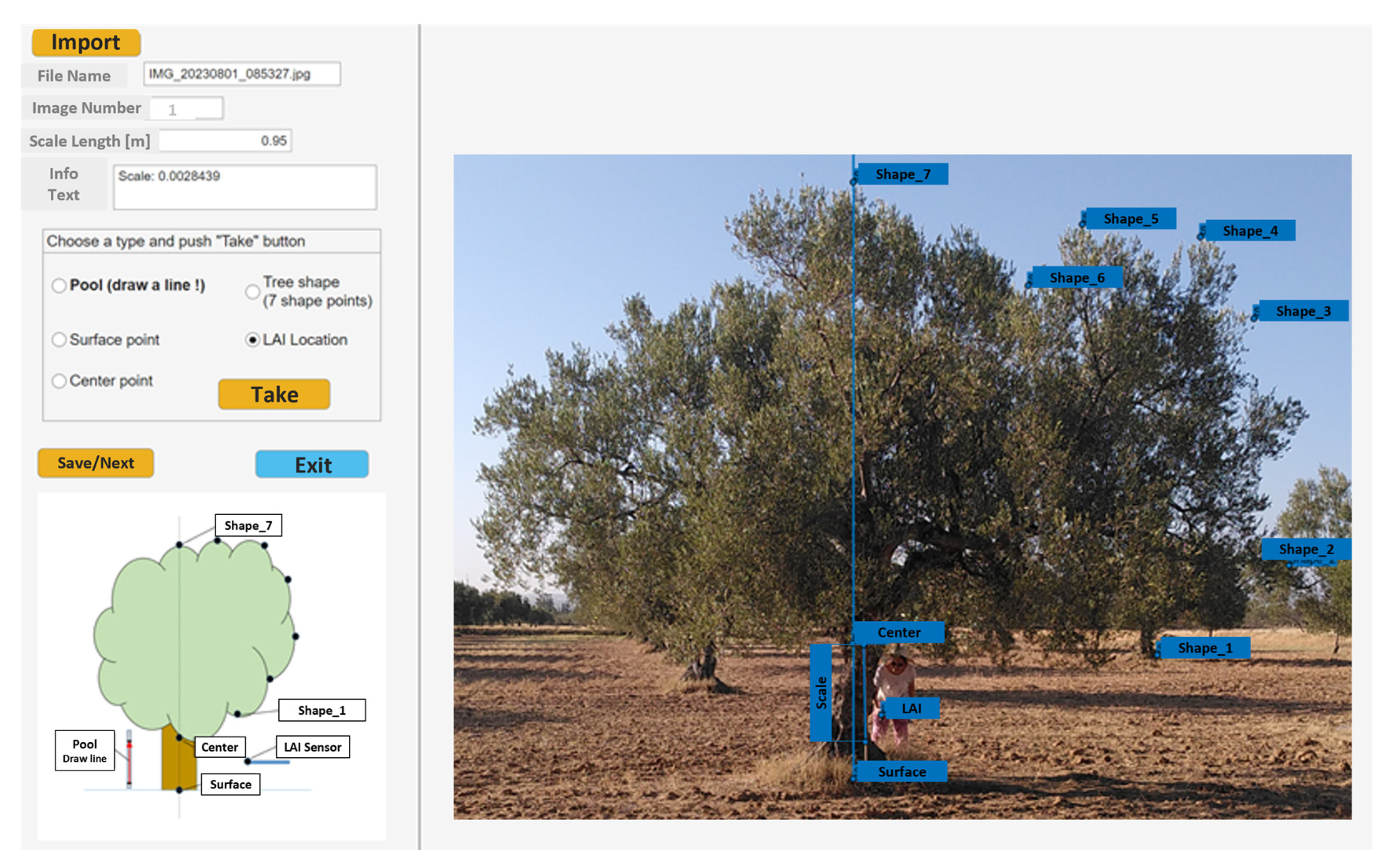
Figure 2. Tree crown shape definition for scatter correction using a custom MATLAB script in FV2200 LAI post-processing.
Remotesensing 18 01300 g002
Figure 3. Left-hand side: Workflow diagram for automatic tree top position and digital terrain model calculation (by applying structure from motion (SFM), cloth simulation filter (CSF), locally estimated scatterplot smoothing (LOESS), and local maximum filter). Right-hand side: Structural and spectral parameter extraction for individual olive trees from the dense cloud model (by applying density-based spatial clustering of applications with noise (DBSCAN), 2D/3D convex hull, and spectral index calculation).
Remotesensing 18 01300 g003
Figure 4. Tree height model (line) with its confidence interval (shaded area) for two olive orchards in Tunisia depending on the number of points per tree.
Remotesensing 18 01300 g004
Figure 5. Projected crown area model (line) with its confidence interval (shaded area) for two olive orchards in Tunisia depending on the number of points per tree.
Remotesensing 18 01300 g005
Figure 6. Crown volume model (line) with its confidence interval (shaded area) for two olive orchards in Tunisia depending on the number of points per tree.
Remotesensing 18 01300 g006
Figure 7. LAI model (line) with its confidence interval (shaded area) for two olive orchards in Tunisia depending on the number of points per tree.
Remotesensing 18 01300 g007
Figure 8. Predicted parameters, including tree height (A), projected crown area (B), crown volume (C), LAI (D), and NGRDI (E), for the olive orchard in Jammel, 2022.
Remotesensing 18 01300 g008
Figure 9. Predicted parameters, including tree height (A), projected crown area (B), crown volume (C), LAI (D), and NGRDI (E), for the olive orchard in Toukaber, 2023.
Remotesensing 18 01300 g009
Table 1. Mean reference values with standard deviation for olive trees of the field campaigns in 2022 and 2023.
SiteYearTree Height [m]SPAD Value
[-]
Tree Crown Volume [m3]Projected Crown Area [m2]LAI [-]
Jammel20225.55 ± 0.4382.00 ± 1.4634.39 ± 12.8211.28 ± 3.360.35 ± 0.12
20235.33 ± 0.5484.52 ± 1.6138.93 ± 14.6413.07 ± 3.830.49 ± 0.15
Toukaber20222.64 ± 0.4284.33 ± 2.133.49 ± 2.162.02 ± 0.841.48 ± 0.24
20232.32 ± 0.3085.31 ± 1.462.08 ± 0.841.42 ± 0.521.71 ± 0.44
Table 2. Model result overview for the different tree parameter estimations for data subsets of trees represented by a high and low number of points in the dense point cloud for two olive orchards in Tunisia.
High Number of PointsLow Number of Points
ParameterR2RMSEBox-Cox TransformationR2RMSEBox-Cox Transformation
Tree height0.890.52 m/0.880.54 m/
Proj. crown area 0.822.40 m2 λ = 0.3140.911.38 m2 λ = 0.686
Crown volume0.856.48 m3 λ = 0.6480.914.26 m3 λ = 0.209
LAI0.730.26 λ = 0.0300.680.35 λ = 0.055
SPADModel rejected
Table 3. Parameter significance, standard error (SE), confidence interval (CI) boundaries, and influence of the tree crown volume model for two olive orchards in Tunisia grouped by number of points per tree (high: n = 75; low: n = 30).
High Number of PointsLow Number of Points
TermMultiplierSECI95%
LB
CI95%
HB
Probabil. > |t|MultiplierSECI95%
LB
CI95%
HB
Probabil. > |t|
Intercept9.001.795.4312.57<0.0001 *3.511.680.066.960.0464 *
Raster (0.05 m)3.042.30−1.557.630.19112.846.20−9.8815.560.6505
Volume0.120.0110.0980.14<0.0001 *0.200.0150.170.23<0.0001 *
Interaction (Raster * Volume)−0.060.011−0.085−0.043<0.0001 *−0.180.057−0.3−0.0670.0032 *
* Bold numbers: significant influence of parameters according to 95% confidence interval.
Table 4. Parameter significance, standard error (SE), confidence interval (CI) boundaries, and influence of the LAI model for two olive orchards in Tunisia grouped by number of points per tree (high; n = 75; low: n = 30).
High Number of PointsLow Number of Points
TermMultiplierSECI95%
LB
CI95%
HB
Probabil. > |t|MultiplierSECI95%
LB
CI95%
HB
Probabil. > |t|
Intercept0.100.072−0.0480.240.18640.150.14−0.130.430.2699
Raster (0.05 cm)0.0290.093−0.160.210.7580−0.170.50−1.200.860.7328
Volume−0.00360.00044−0.005−0.003<0.0001 *−0.00830.0012−0.011−0.006<0.0001 *
Interaction (Raster * Volume)0.00290.000420.0020.004<0.0001 *0.0190.00460.0090.0280.0004 *
* Bold numbers: significant influence of parameters according to the 95% confidence interval.
Disclaimer/Publisher’s Note: The statements, opinions and data contained in all publications are solely those of the individual author(s) and contributor(s) and not of MDPI and/or the editor(s). MDPI and/or the editor(s) disclaim responsibility for any injury to people or property resulting from any ideas, methods, instructions or products referred to in the content.