A Fine-Scale Urban Impervious Surface Extraction Method Based on UAV LiDAR and Visible Imagery

Highlights

What are the main findings?

• The proposed EGS-Optimizer significantly improves segmentation quality compared with the traditional ESP2 multi-scale segmentation approach in object-based image analysis (OBIA).
• The integration of UAV visible imagery and UAV-LiDAR data, combined with SHAP-based feature selection, effectively improves impervious surface classification performance, achieving an overall accuracy of 97.24% (Kappa = 0.96).

What are the implications of the main findings?

• Multi-source data fusion can effectively reduce spectral ambiguity among complex urban land-cover types by incorporating complementary spectral and structural information.
• The proposed framework demonstrates strong performance for fine-scale impervious surface extraction within the local study area.

Abstract

Accurate extraction of impervious surface areas (ISA) is essential for urban environmental monitoring, yet severe spectral confusion among complex urban land-cover types limits the performance of classifications based solely on optical imagery. To address this issue within a localized context, this study proposes a multi-source framework integrating UAV-based LiDAR (UAV-LiDAR) and high-resolution visible imagery for fine-scale ISA extraction. An improved segmentation optimization strategy, termed EGS-Optimizer, is developed to enhance boundary delineation within the object-based image analysis (OBIA) framework by coupling edge detection with global segmentation quality evaluation. A comprehensive feature set including spectral, index, texture, geometric, and terrain features is constructed, and Shapley Additive Explanations (SHAP) is applied to select the most informative variables while reducing dimensionality. The proposed framework is validated in a typical 1.45 km² built-up area in Deyang City, Sichuan Province. Experimental results demonstrate that, within this specific study area, multi-source data fusion improves classification accuracy by 3.59–5.79% compared with single-source data, while feature selection reduces the feature dimension from 45 to 21. Among the evaluated classifiers, the random forest (RF) model achieves the highest performance, with an overall accuracy of 97.24% (Kappa = 0.96). While the high accuracy highlights the efficacy of synergizing spectral and structural information for micro-landscape mapping, these findings are constrained to the demonstrated fine-scale local environment. The results provide an effective, interpretable solution for detailed neighborhood-level ISA mapping, though further validation is required before the framework can be generalized to larger or more heterogeneous urban scenarios.

1. Introduction

Urban impervious surface areas [1] refer to land surfaces covered by artificial materials that permit little or no water infiltration, such as rooftops, roads, and parking lots. With the acceleration of urbanization, impervious surfaces continue to expand, disrupting watershed hydrological cycles [2], intensifying non-point source pollution [3] and urban heat island effects [4], and exerting adverse impacts on urban biodiversity and ecological security [5,6]. Therefore, accurate and efficient acquisition of ISA spatial distribution is essential for urban ecological monitoring, land-use planning, and carbon neutrality assessments.

The development of ISA extraction is driven by advancements in remote sensing data and algorithms. Early studies predominantly relied on medium- and high-resolution optical satellite imagery [7,8,9]. At the medium-resolution scale, spectral indices and pixel-based classifiers achieved moderate success in large-scale urban mapping [10]. As the field progressed to high-resolution optical imagery (e.g., WorldView, QuickBird), the focus shifted toward mitigating the “salt-and-pepper” effect, leading to the widespread adoption of object-based image analysis (OBIA) [11,12] and machine learning algorithms. However, despite these algorithmic advancements, optical imagery inherently faces severe spectral confusion between impervious surfaces and bare soil [13], coupled with inherent limitations under adverse weather conditions and shadow interference.

To overcome the spectral and weather limitations of single-source optical data, the field progressed into the era of multi-source data fusion, initially marked by the integration of optical and Synthetic Aperture Radar (SAR) data [14]. SAR provides all-weather, day-and-night observation capabilities, and its backscatter characteristics effectively complement optical spectra, significantly improving extraction accuracy in cloud-prone or complex urban areas [15]. Building upon this, the fusion of optical imagery and LiDAR data emerged as another critical milestone [16]. Unlike SAR, airborne LiDAR provides precise vertical structural information, which fundamentally resolves the spectral confusion between elevated impervious surfaces (e.g., rooftops, roads overpasses) and non-impervious features with similar spectral signatures (e.g., bare soil, low vegetation) [17]. This progression from optical-SAR to optical-LiDAR fusion necessitated distinct algorithmic adaptations at each stage to handle heterogeneous data structures.

Despite the success of spaceborne and airborne multi-source fusion, satellite-based platforms are still constrained by spatial resolution and revisit cycles [18], restricting their ability to perform fine-grained analysis of highly fragmented urban morphologies. This inherent limitation has driven the rapid development of Unmanned Aerial Vehicle (UAV)-based remote sensing methods. UAV platforms acquire ultra-high-resolution (centimeter-level) optical imagery and dense UAV-LiDAR point clouds, offering an unprecedented capability to delineate tiny, heterogeneous impervious features at the micro-landscape scale. However, the shift to UAV multi-source fusion introduces new algorithmic challenges. For instance, conventional OBIA, widely used in high-resolution imagery, struggles with scale parameter selection in ultra-high-resolution data. While tools like the Estimation of Scale Parameter 2 (ESP2) plugin are commonly used, they often rely on visual interpretation, resulting in strong subjectivity [19]. Although prior studies [20,21] have explored edge detection and global segmentation quality (GS) indices independently, explicitly integrating edge information with segmentation quality assessment within a unified optimization framework remains underexplored for UAV data.

In addition, the fusion of high-resolution optical imagery and LiDAR data produces high-dimensional feature spaces, which may introduce redundancy and affect classification stability [22,23]. Recently, Shapley Additive Explanations (SHAP) [24], a game-theory-based interpretability method, has been widely used for feature importance evaluation and feature selection. It enables effective reduction of redundant features while preserving model performance, thereby improving classification robustness [25].

To address the above challenges, this study proposes a refined framework for fine-scale urban impervious surface extraction by integrating UAV-LiDAR and high-resolution visible imagery. Building upon the conventional ESP2 scale selection approach, an improved EGS-Optimizer is developed, which incorporates edge detection into the segmentation parameter optimization process by coupling it with global segmentation quality assessment. This strategy enhances boundary delineation and improves the objectivity of scale selection. A multi-source feature system is constructed, including spectral, index, textural, geometric, and topographic features, and SHAP-based feature selection is applied to identify the most informative variables, thereby reducing redundancy and improving model interpretability. Multiple classifiers, including k-nearest neighbors (KNN), decision tree (DT), support vector machine (SVM), RF and extreme gradient boosting (XGBoost), are evaluated under different feature schemes to assess the effectiveness of the proposed method.

The proposed framework is specifically designed for fine-scale urban impervious surface extraction using high-resolution multi-source data. Within this context, the multi-class land-cover procedure is not intended as a general-purpose classification task but rather serves as a targeted technical pathway to accurately delineate impervious surfaces—especially resolving spectral confusion with bare soil. Ultimately, the findings provide valuable support for detailed ISA mapping in localized urban environments, facilitating applications such as urban micro-environment analysis, stormwater management, and urban planning.

2. Study Area and Data Sources

2.1. Study Area

The study area is located in the urban core of Jingyang District, Deyang City, Sichuan Province, within the geographic coordinates of 30–35°N and 100–105°E, covering approximately 1.45 km² (Figure 1). The terrain is generally flat and represents a typical built-up area of an inland basin city in Southwest China. The land cover is diverse, including roads, buildings, sports fields, grasslands, bare soil, and trees, exhibiting pronounced spatial heterogeneity and complexity. Buildings are densely distributed with significant variations in height, and several neighborhoods feature mixed patterns of high- and low-rise structures, shaping a distinct three-dimensional urban form. In addition, an intertwined road network, open sports grounds, and diverse vegetation types pose considerable challenges for impervious surface extraction. This typicality and complexity provide a representative experimental setting for validating the proposed fine-scale methodology within a localized context.

Therefore, the area is selected to explore how multi-source data integration and feature optimization can address the challenges of fine-scale ISA extraction in complex urban environments.

2.2. Data Sources

The data used in this study are acquired by a Feima D2000 UAV (Feima Robot, Beijing, China) equipped with multisource sensors. Visible imagery is collected using a Sony A7R IV camera (Sony, Tokyo, Japan) (sensor size 35.7 × 23.8 mm, 61 megapixels, 40 mm focal length) at a flight altitude of 500 m, with forward and side overlaps of 80% and 75%, respectively, and a flight speed of 13.5 m/s. LiDAR data are obtained using the D-LiDAR2000 system (Feima Robot, Beijing, China) (wavelength 905 nm) at the same altitude, with both forward and side overlaps of 70% and a flight speed of 9 m/s. The integration of UAV visible imagery and LiDAR data is used to generate a Digital Orthophoto Map (DOM), a digital surface model (DSM), a digital elevation model (DEM), and intensity features (INT). The data preprocessing process is shown in Figure 2.

3. Experimental Methods

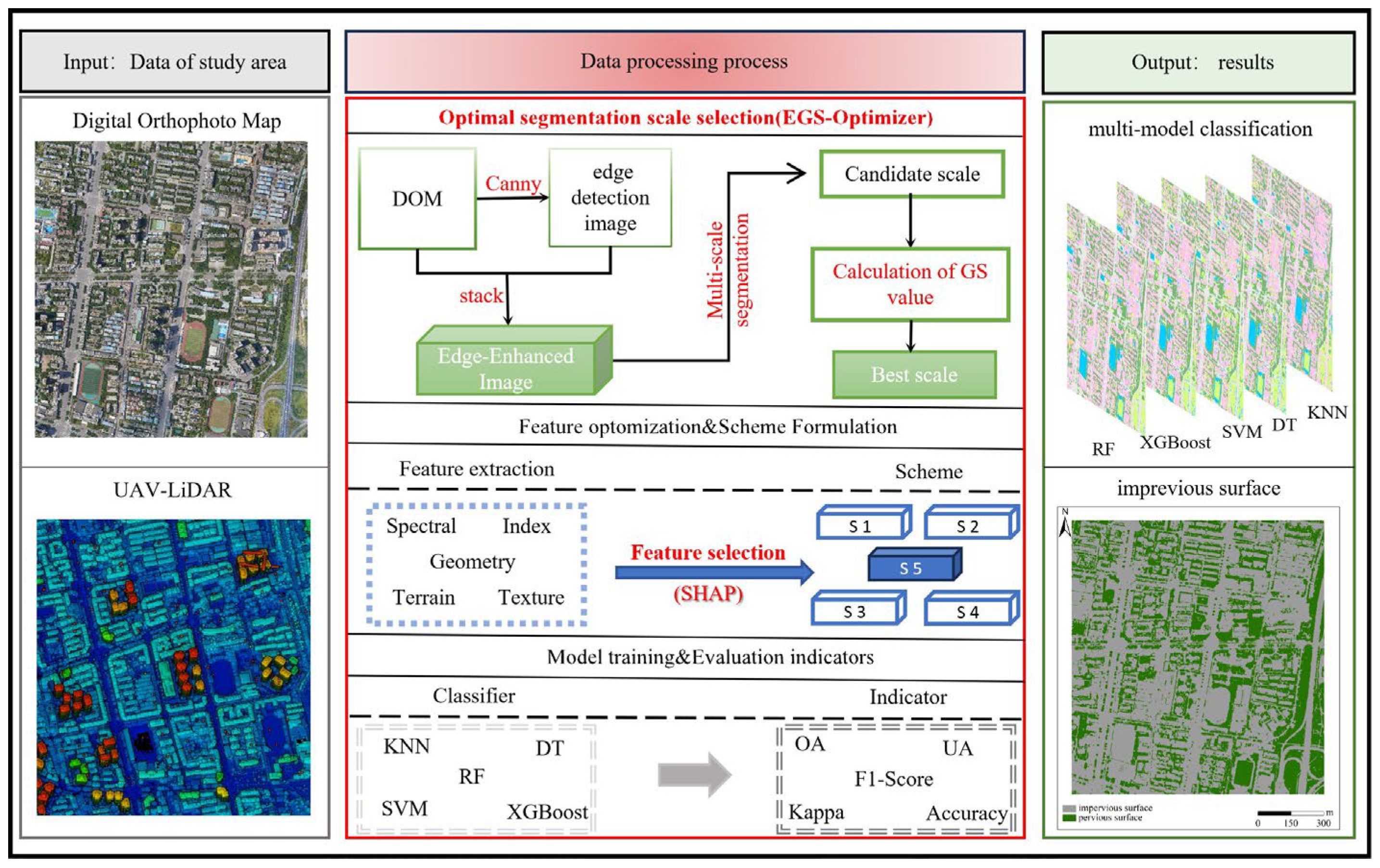
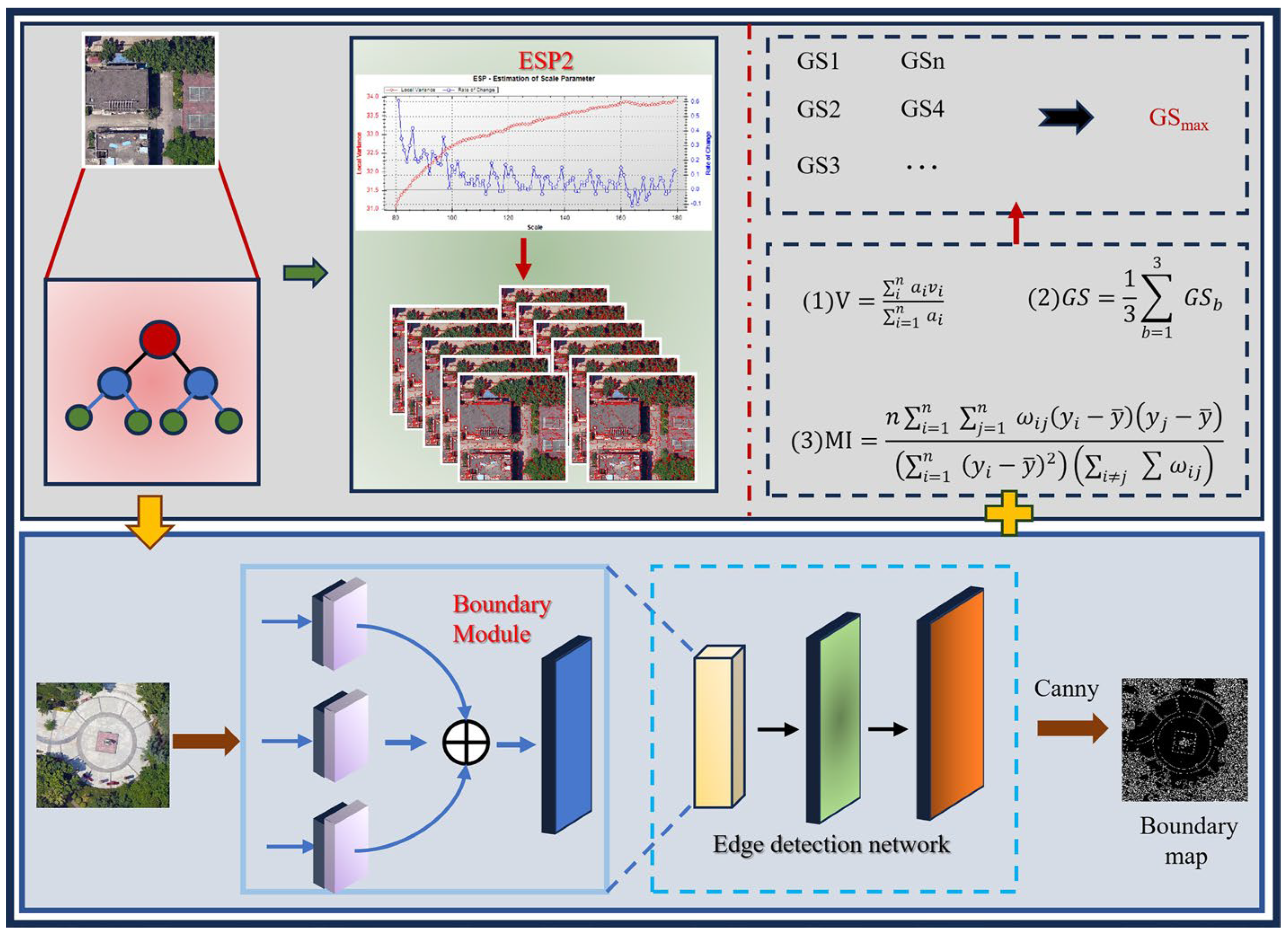
The methodological framework of this study is illustrated in Figure 3 and consists of three main components: data preparation, data processing, and classification results.

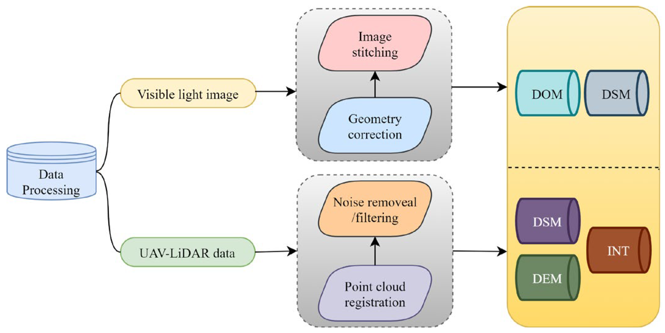
First, UAV visible imagery and LiDAR point cloud data are acquired to construct a multisource data fusion framework. Next, to optimize the object-based analysis, the EGS-Optimizer is applied: edge detection results are first directly concatenated with the visible imagery as additional bands to construct an enhanced feature space; the ESP2 tool is then executed on this edge-enhanced dataset for initial scale estimation; finally, the GS index is used to quantitatively filter the candidate scales. Based on the optimal segmentation scale determined by this process, multidimensional features of six land-cover classes are extracted. On this basis, SHAP is applied for feature selection, and five experimental schemes (S1–S5) are designed. Finally, the classification performance of different models is compared across the schemes, and impervious surfaces are optimally extracted under the best-performing configuration.

3.1. Segmentation Optimization Method

Image segmentation constitutes the core of Object-Based Image Analysis (OBIA), and the rationality of scale selection directly affects boundary preservation, subsequent feature extraction, and classification outcomes. Traditional OBIA techniques often employ the ESP2 tool [20] for scale determination; however, they still rely heavily on visual interpretation, which introduces subjectivity and limits quantitative evaluation. Aiming to improve the scientificity and adaptability of traditional methods, this paper proposes an scale-adaptive optimization method (EGS-Optimizer) for object-oriented image segmentation. By injecting boundary gradients directly into the input data, the segmentation algorithm inherently adjusts its heterogeneity criteria to respect object boundaries during the region-growing process. Finally, candidate scales generated from this edge-embedded segmentation are quantitatively filtered using the GS index, complemented by visual inspection, to determine the final optimal segmentation scale.

(1) Edge detection

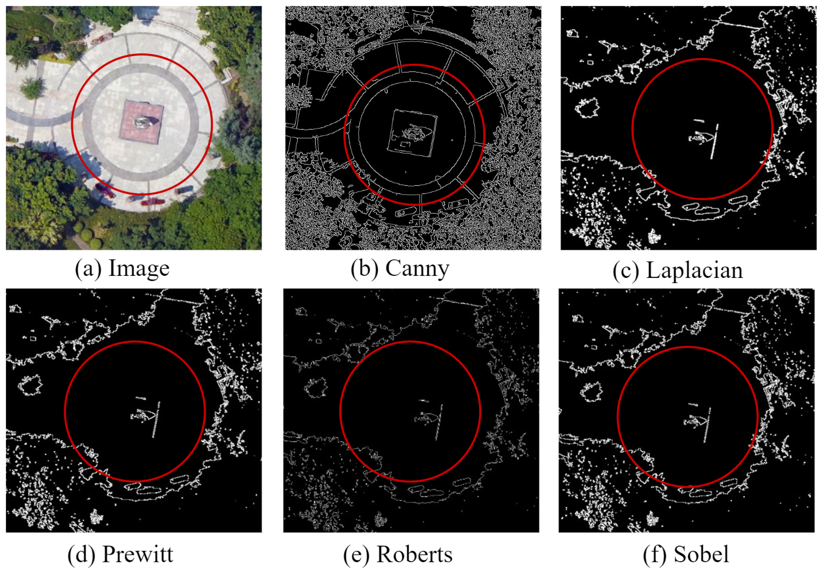
Edge detection is a fundamental task in image processing, aiming to identify pixels where brightness or texture changes abruptly, thereby delineating the contours and boundaries of surface objects. In object-based image analysis (OBIA) with high-resolution remote sensing imagery, the integration of precise edge information effectively constrains the segmentation process and significantly improves both boundary accuracy and internal homogeneity of image objects. In this study, five commonly used operators—Canny, Roberts, Prewitt, Sobel, and Laplacian—are applied to local subsets of the original imagery for edge detection [26]. As observed in Figure 4, especially in the highlighted regions, the ground objects segmented using the Canny operator exhibit shapes that more closely conform to their real-world geometry, outperforming those obtained by other operators. Consequently, it is adopted as the primary edge detection method in this work. 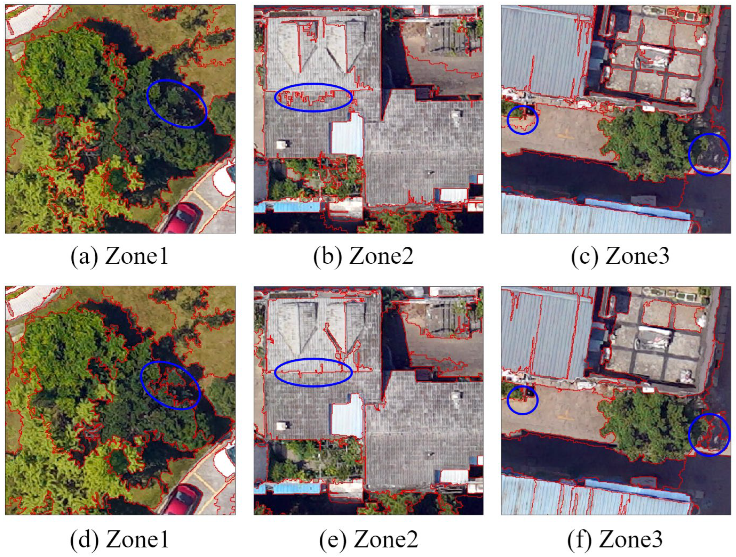As illustrated in Figure 5, the incorporation of edge detection markedly enhances the segmentation results.

(2) Global segmentation quality evaluation indicators

The global segmentation quality (GS) index integrates the within-object standard deviation (V) and the spatial autocorrelation (Moran’s I) [27] to quantitatively assess different segmentation scales, thereby identifying the optimal balance between intra-object consistency and inter-class separability. Substantial variation in GS values is observed across segmentation scales, with higher GS values generally indicating superior segmentation quality [28].The numerical variability is determined using the standard deviation function within the object, as shown in Equation (1).

$$\mathrm{V}={\displaystyle \frac{\sum _i^n a_i{v}_i}{\sum _{i=1}^n a_i}}$$

(1)

where $n$ is the number of objects after segmentation, $v_i$ denotes the internal standard deviation of object $i$, $a_i$ represents the area of object $i$.

The spatial dependency is determined using a spatial autocorrelation function, as shown in Equation (2).

$$\mathrm{M}\mathrm{I}={\displaystyle \frac{n\sum _{i=1}^n \sum _{j=1}^n {\omega }_{ij}\left(y_i-\overline{y}\right)\left(y_j-\overline{y}\right)}{\left(\sum _{i=1}^n {\left(y_i-\overline{y}\right)}^2\right)\left(\sum _{i\ne j} \sum {\omega }_{ij}\right)}}$$

(2)

where $n$ is the number of segmented objects, ${\omega }_{ij}$ represents the weight matrix; $y_i$ and $y_j$ denote the mean values of $i$ and $j$ respectively, and $y$ is the global mean value of the entire image.

The selection of the segmentation scale is determined using a global segmentation quality evaluation metric function, as shown in Equation (3).

$$\mathrm{G}\mathrm{S}={\displaystyle \frac{1}{3}}\sum _{b=1}^3 G{S}_b$$

(3)

where $G{S}_b$ is defined as the sum of the normalized internal standard deviation V and the Moran’s Index (MI) for the object and $b$ denotes the spectral band involved in the segmentation.

(3) EGS-Optimizer workflow (Figure 6)

The core concept of the EGS-Optimizer lies in enhancing object boundary recognition through edge detection while comprehensively evaluating the rationality of segmentation scales using the GS index. In this study, the ESP2 tool is first employed for initial scale estimation, with reference to previous research on impervious surface extraction [20], where the shape factor and compactness parameters are set to 0.1 and 0.5, respectively. The segmentation scale is determined by assessing object homogeneity indicators [29], specifically local variance (LV) and its rate of change (ROC), to quantify spectral consistency variations across different scales. This facilitates objective, data-driven parameter selection. Subsequently, edge detection is applied to enhance object boundary delineation and optimize segmentation results. Finally, candidate scales are quantitatively filtered using the GS index, complemented by visual inspection, to determine the final optimal segmentation scale.

A comparative analysis delineating the paradigm shifts between the proposed strategy and existing methods is presented in

Table 1. Comparison of EGS-Optimizer and existing segmentation methods.

Method	Scale Selection	Edge Information	Evaluation Metric	Integration Strategy
ESP2	√	×	Local variance	Visual interpretation
ESP2 + GS	√	×	GS index	Post-evaluation
Edge-based- Segmentation	×	√	None	Independent
EGS-Optimizer	√	√	GS index	Feature-level embedding

. Conventional ESP2-based methods determine the optimal segmentation scale primarily through local variance analysis and visual interpretation, which inherently introduces subjectivity. The ESP2 + GS approach mitigates this by introducing the global segmentation quality (GS) index [30]; however, it treats the optimization process as a purely global, semantic evaluation, creating a structural blind spot for local boundary fidelity. Conversely, edge-based segmentation methods excel at boundary detection but are typically relegated to an independent post-processing step or act as a loose auxiliary constraint, lacking a systematic mechanism to actively govern the scale optimization loop.

To resolve this dichotomy between global scale evaluation and local edge preservation, the EGS-Optimizer shifts the operational level of edge information from the output stage to the input stage. Rather than using edges to passively refine results after segmentation (post-processing), or evaluating them in isolation, the EGS-Optimizer embeds edge features directly into the image segmentation space as foundational input bands. This feature-level embedding ensures that local boundary gradients inherently govern the region-growing process during multi-scale segmentation. Consequently, edge information is transformed from a peripheral post-processing filter to a primary segmentation driver, allowing the subsequent GS index to evaluate scales that are already optimized for boundary fidelity.

Consequently, edge features are transformed from a peripheral auxiliary feature to a core optimization component within a unified objective function. This mechanism enables the proposed method to achieve simultaneous boundary delineation and scale consistency, particularly for fine-scale urban objects. It should be emphasized that the EGS-Optimizer acts as a foundational enhancement to existing frameworks—not merely by appending edge information, but by restructuring how edge constraints actively drive the scale optimization process.

3.2. Feature Extraction

Based on the optimal segmentation results, multidimensional features are extracted for six object categories. These include:

(1) Spectral features: mean values of the red (Mean_R), green (Mean_G), and blue (Mean_B) bands, edge detection results derived from the Canny operator, brightness, and the maximum inter-band difference (Max_diff).

(2) Index features (

Table 2. Index formula.

Index	Formula	References
DEVI	${\displaystyle \frac{G+B+R}{3G}}$	[31]
EXG	$2G-B-R$	[32]
EXGR	$2G-B-R-(1.4R-G)$	[33]
EXR	$1.4R-G$	[34]
GBRI	${\displaystyle \frac{B}{G}}$	[21]
GVI	${\displaystyle \frac{G}{R+G+B}}$	[35]
MGRVI	${\displaystyle \frac{G^2-R^2}{G^2+R^2}}$	[36]
NGBDI	${\displaystyle \frac{G-B}{G+B}}$	[37]
NGRDI	${\displaystyle \frac{G-R}{G+R}}$	[38]
RGBVI	${\displaystyle \frac{G^2-BR}{G^2+BR}}$	[36]
VDVI	${\displaystyle \frac{2G-R-B}{2G+R+B}}$	[38]

Note: R, G and B denote the red, green, and blue bands of the visible imagery, respectively.

)

(3) Texture features (

Table 3. Texture formula.

Texture	Formula
Homogeneity	$\mathrm{Homogeneity}={\displaystyle \sum _{i=1}^{N_g}} {\displaystyle \sum _{j=1}^{N_g}} {\displaystyle \frac{P(i,j)}{1+(i-j{)}^2}}$
Entropy	$\mathrm{Entropy}=-{\displaystyle \sum _{i=1}^{N_g}} {\displaystyle \sum _{j=1}^{N_g}} P(i,j)\mathrm{l}\mathrm{o}\mathrm{g}P(i,j)$
Correlation	$\mathrm{Correlation}={\displaystyle \frac{{\sum }_{i=1}^{N_g} {\sum }_{j=1}^{N_g} \left(i-{\mu }_i\right)\left(j-{\mu }_j\right)P(i,j)}{{\sigma }_i{\sigma }_j}}$
Standard Deviation	$\mathrm{Std}=\sqrt{{\displaystyle \sum _{i=1}^{N_g}} {\displaystyle \sum _{j=1}^{N_g}} p(i,j)\ast (i- \mathrm{Mean}{)}^2}$
Contrast	$\mathrm{Contrast}={\displaystyle \sum _{i=1}^{N_g}} {\displaystyle \sum _{j=1}^{N_g}} (i-j{)}^{2}P(i,j)$
Dissimilarity	$\mathrm{Dissimilarity}={\displaystyle \sum _{i=1}^{N_g}} {\displaystyle \sum _{j=1}^{N_g}} P(i,j)\cdot |i-j|$
Angular Second Moment	$\mathrm{A}\mathrm{S}\mathrm{M}={\displaystyle \sum _{i=1}^{N_g}} {\displaystyle \sum _{j=1}^{N_g}} P(i,j{)}^2$
Mean	$\mathrm{Mean}={\displaystyle \sum _{i=1}^{N_g}} {\displaystyle \sum _{j=1}^{N_g}} i\cdot P(i,j)$

)

(4) Geometric features: Seventeen features are extracted, including Area, Length, Width, Border Length, Shape Index, Density, Main Direction, Asymmetry, and Rectangular Fit, among others.

(5) Terrain features: These include height features (HEIG) and intensity features (INT). The height features consist of two types: the digital normalized digital surface Model (DNDSM) directly generated from UAV orthophotos and the normalized digital surface model (NDSM) derived from the fusion of visible imagery and LiDAR data [39].

$$\mathrm{N}\mathrm{D}\mathrm{S}\mathrm{M}=DSM-DEM$$

(4)

3.3. Sample Selection

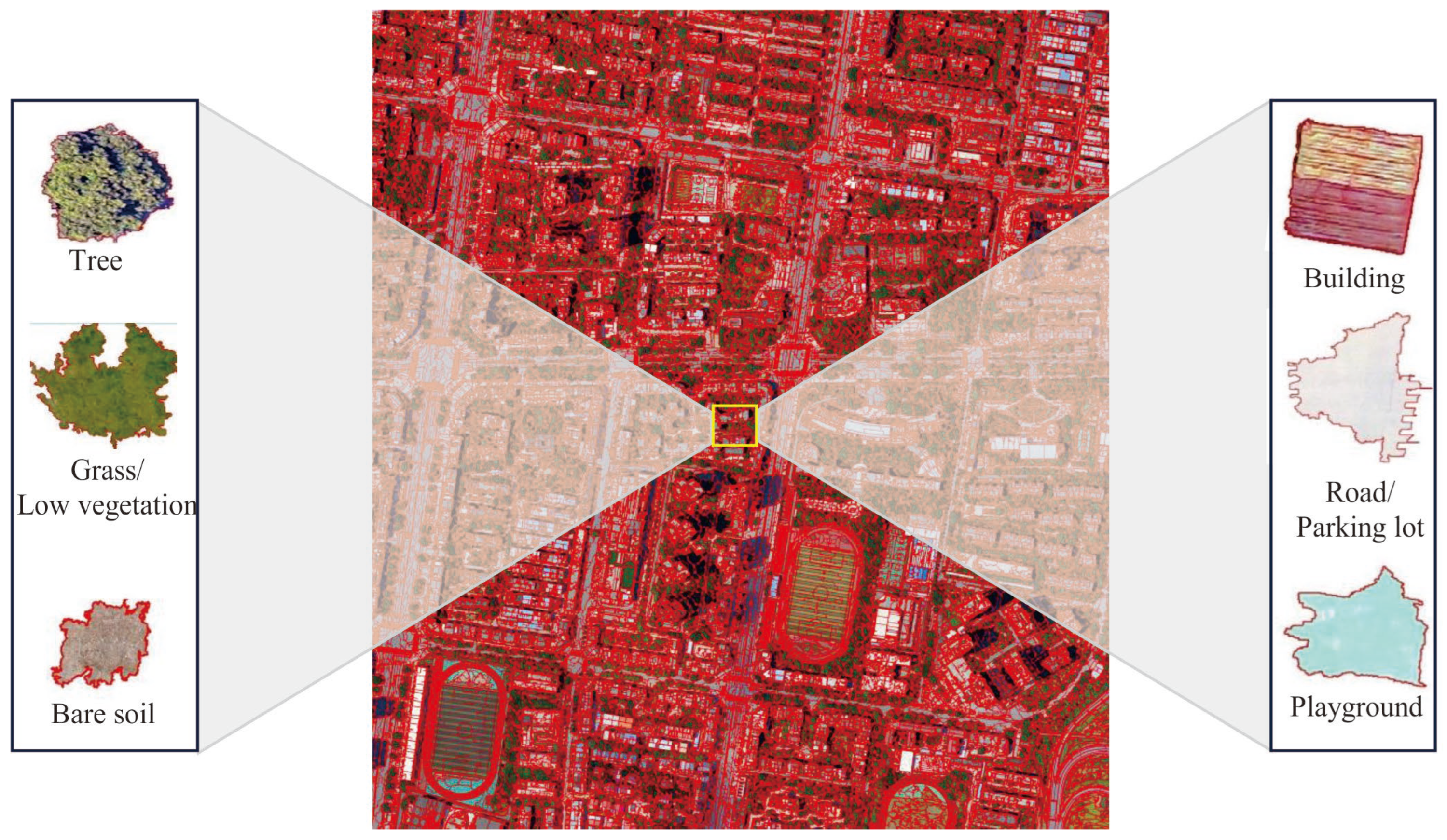
Based on the characteristics of UAV imagery and land-cover distribution in the study area, six object classes are defined: trees, buildings, roads/parking lots, sports fields, grass/low vegetation, and bare soil (Figure 7). Sample numbers for each class are determined using random sampling (

Table 4. Sample numbers for each land-cover class.

Object Type	Total Sample	Training Sample	Validation Sample
Tree	890	603	285
Building	1648	1152	495
Road/Parking lot	846	609	236
Playground	520	359	161
Grass/Low vegetation	808	567	241
Bare soil	135	100	35

) and are split into training and validation sets at a 7:3 ratio to support subsequent model training and accuracy assessment [40].

3.4. Feature Optimization

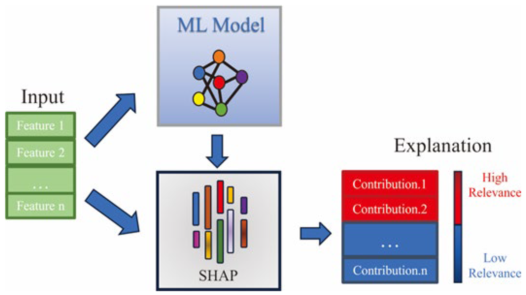
In machine learning, some features may exhibit strong correlations or redundancies, meaning that certain information can be inferred from other features. Such redundant features not only fail to significantly improve model performance but also increase computational complexity, reduce training efficiency, and negatively affect model generalization [5]. To address this issue, SHAP is employed for feature selection in this study (Figure 8).

Based on the game-theoretic Shapley values, SHAP quantifies the marginal contribution of each feature to the model’s predictions and combines global and local interpretability. Features with higher SHAP values are considered to have a greater impact on the model’s predictive outcomes.

3.5. Scheme Formulation and Evaluation Indicators

3.5.1. Scheme Formulation

To investigate the influence of different feature combinations on urban impervious surface classification accuracy, five experimental schemes (

Table 5. Classification scheme.

Scheme	Feature	Number
S1	Visible light	42
S2	Visible light + DNDSM	43
S3	Visible light +NDSM + INT	44
S4	Visible light + HEIG + INT	45
S5	Optimization feature	N

) are designed in this study. Five commonly used machine learning algorithms—KNN, DT, SVM, RF, and XGBoost—are applied to classify the land-cover classes within the study area. Scheme S1 includes only visible features (spectral, index, texture, and geometric features), while schemes S2–S4 progressively incorporate additional topographic and LiDAR-derived features. Specifically, S2 integrates visible imagery with the visible-derived height feature (DNDSM), S3 further incorporates the radar-derived height feature (NDSM) and LiDAR intensity (INT), and S4 replaces the separate height features with a combined height feature (HEIG), defined as the sum of NDSM and DNDSM, together with intensity information. Scheme S5 consists of an optimized feature set derived through SHAP-based feature selection.

3.5.2. Evaluation Indicators

To evaluate the effectiveness of the proposed method, different classification models are selected under each experimental scheme, and the method performance is quantitatively assessed using user’s accuracy (UA), producer’s accuracy (PA), overall accuracy (OA), and the Kappa coefficient. Given the significant sample size imbalance among certain classes (e.g., bare soil versus buildings, as detailed in Table 4), relying solely on user’s accuracy (UA) and producer’s accuracy (PA) may lead to biased assessments. To address this issue, the F1-score is introduced as a complementary evaluation metric. By integrating precision (UA) and recall (PA) through their harmonic mean, the F1-score provides a more balanced and robust assessment of classification performance, particularly for minority classes. The corresponding formulas are provided in Equations (5)–(10)

$$\mathrm{O}\mathrm{A}={\displaystyle \frac{\sum _{i=1}^n {TP}_i}{N}}$$

(5)

$${\mathrm{P}\mathrm{A}}_i={\displaystyle \frac{{TP}_i}{{TP}_i+{FN}_i}}$$

(6)

$${\mathrm{U}\mathrm{A}}_i={\displaystyle \frac{{TP}_i}{{TP}_i+{FP}_i}}$$

(7)

$$P_e={\displaystyle \frac{1}{N^2}}\sum _{i=1}^n\left(T{P}_i+F{N}_i\right)\times \left(T{P}_i+F{P}_i\right)$$

(8)

$$\mathrm{K}\mathrm{a}\mathrm{p}\mathrm{p}\mathrm{a}={\displaystyle \frac{OA-P_e}{1+P_e}}$$

(9)

$$\mathrm{F}1=2\times (UA\times PA)/(UA+PA)$$

(10)

where true positive ${(TP}_i)$: the number of samples correctly classified as class $i$, true negative ${(TN}_i)$: the number of samples not belonging to class $i$ that are correctly classified as other classes, false positive ${(FP}_i)$: the number of samples not belonging to class $i$ that are misclassified as class $i$, false negative ${ (FN}_i)$: the number of samples belonging to class $i$ that are misclassified as other classes $i$, ${ P}_e$: the expected agreement probability,$n$: he number of classification categories and $N$: the total number of samples.

4. Results and Analysis

4.1. Optimal Segmentation Scale

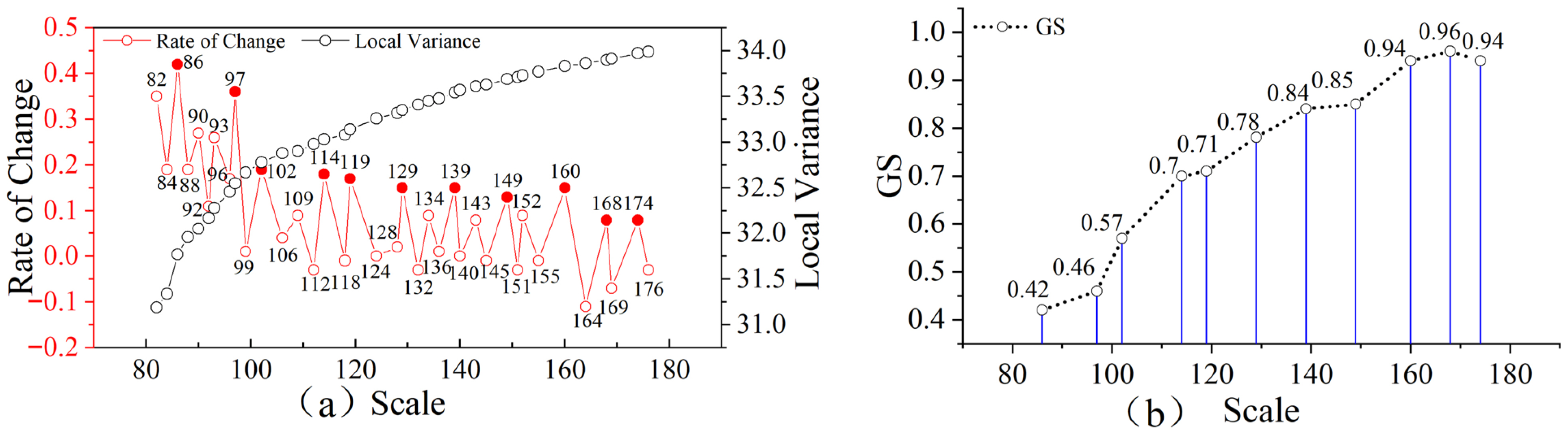
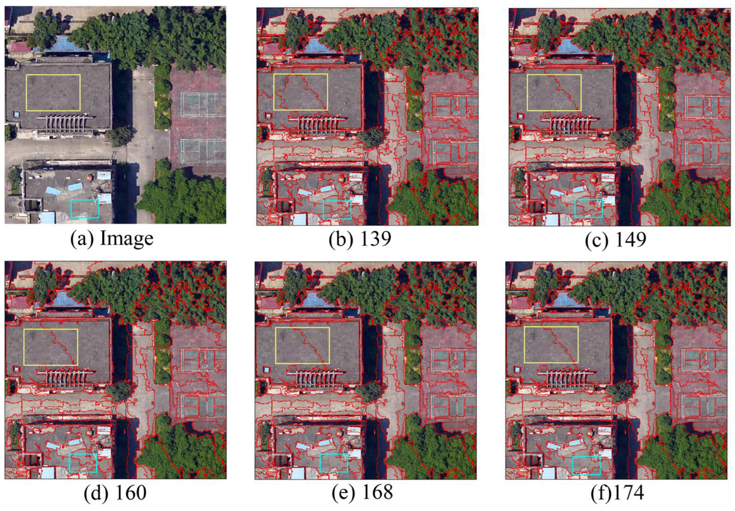
As shown in Figure 9a, the candidate segmentation scales obtained using the ESP2 plugin include 86, 97, 102, 114, 119, 129, 139, 149, 160, 168, and 174. Figure 10 presents a local segmentation comparison of typical land-cover objects. It can be clearly observed, particularly in the highlighted regions marked in the figure, that smaller segmentation scales tend to produce fragmented objects, resulting in over-segmentation. Among the candidate scales, 168 and 174 are very close in value. Therefore, the global segmentation quality (GS) index, as illustrated in Figure 9b, is further used to quantitatively evaluate segmentation performance. The GS value reaches its maximum at a scale of 168, indicating optimal segmentation quality.

This result is consistent with the visual assessment from the highlighted regions in Figure 10, which show that the boundaries of buildings, roads, and vegetation are most clearly and completely delineated at this scale. Therefore, 168 is selected as the optimal segmentation scale and is applied in subsequent feature extraction.

4.2. Feature Optimization Results

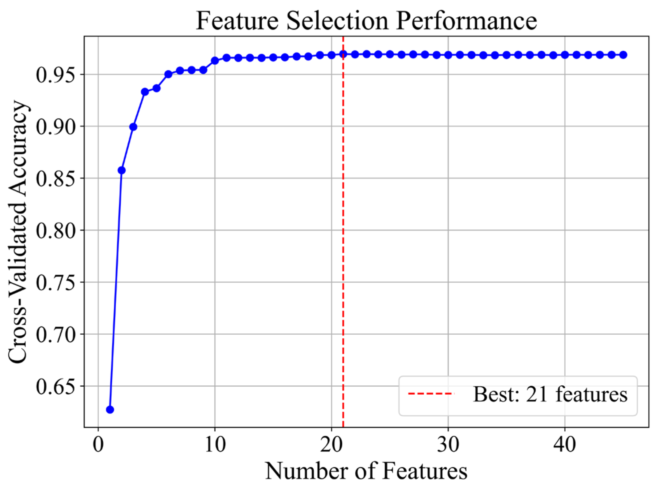
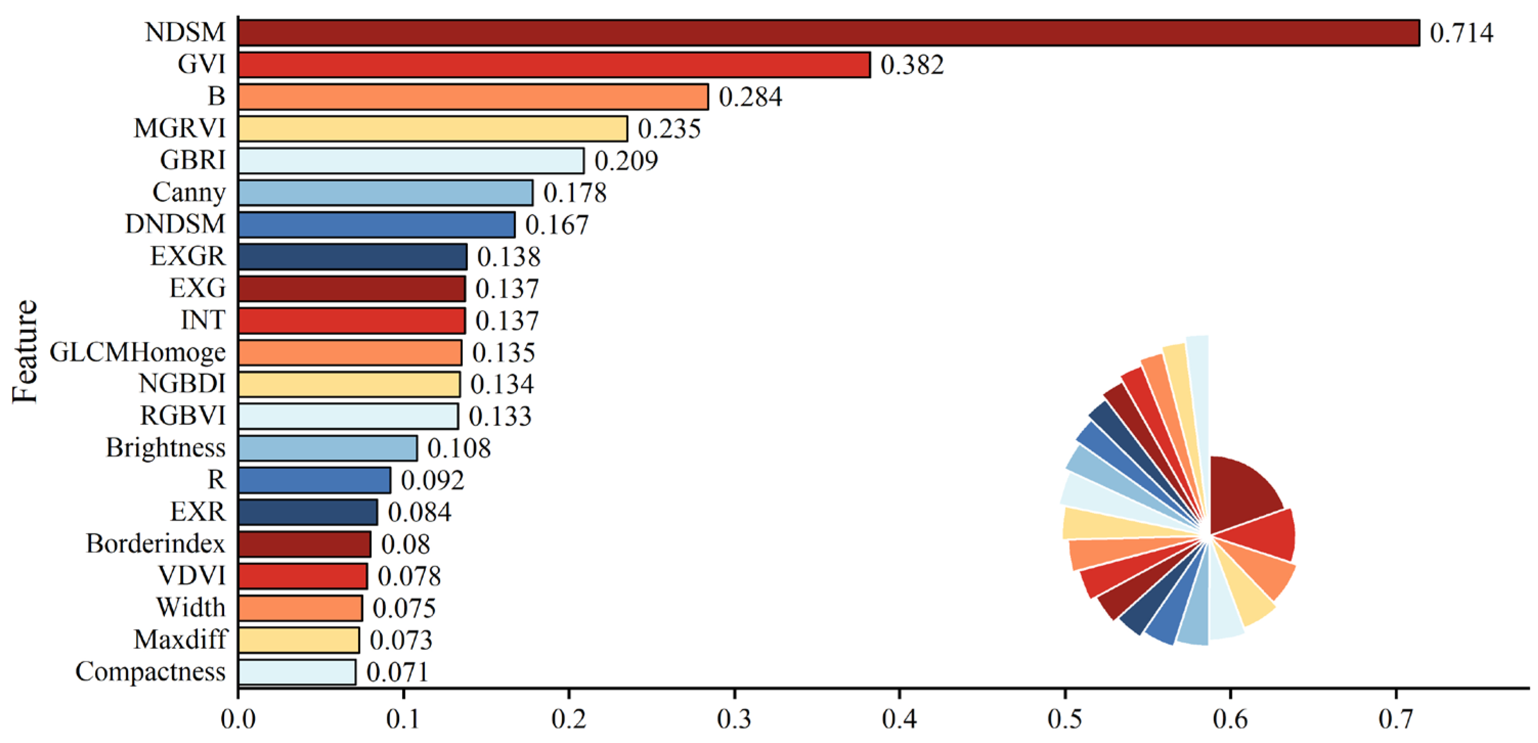
Through SHAP-based feature selection, 45 candidate features are evaluated, and the results indicate that classification accuracy reaches its optimum when 21 features are retained (Figure 11). Among these (Figure 12), the NDSM exhibits the highest importance (0.71), markedly surpassing the DOM-derived DNDSM, which highlights the critical role of LiDAR-derived height features in distinguishing impervious surfaces such as buildings, roads, and bare land. In addition, the intensity feature (0.14) also shows substantial contribution to classification, further underscoring the value of UAV-LiDAR data in impervious surface identification.

4.3. Accuracy Evaluation

4.3.1. Average UA-PA for Land Types

To compare the effects of different feature combinations on classification performance, the average user accuracy (UA) and producer accuracy (PA) of six typical urban land-cover classes under five feature schemes (S1–S5) were calculated (

Table 6. The average UA/PA of the model under each scheme.

Class/Scheme	S1	S2	S3	S4	S5
Tree	0.95/0.97	0.94/0.97	0.95/0.98	0.96/0.98	0.95/0.97
Building	0.86/0.89	0.90/0.92	0.91/0.93	0.92/0.93	0.93/0.92
Road/Parking lot	0.77/0.80	0.82/0.84	0.84/0.86	0.83/0.86	0.85/0.90
Playground	0.92/0.82	0.95/0.84	0.94/0.88	0.93/0.88	0.93/0.93
Grass/Low vegetation	0.94/0.92	0.94/0.94	0.96/0.93	0.96/0.93	0.95/0.93
Bare soil	0.77/0.68	0.78/0.69	0.76/0.68	0.76/0.70	0.79/0.72

). Among these schemes: S1, which includes only visible features, produces the lowest overall accuracy, with substantial confusion between buildings and roads. S2, which introduces visible-light height features (DNDSM) on top of S1, considerably improves the classification accuracy of buildings, roads/parking lots, and sports fields. S3 replaces DNDSM with LiDAR-derived NDSM and intensity features, further enhancing the discrimination between bare soil and grassland. S4 integrates all features, leading to consistent accuracy improvements across land-cover types, with UA/PA values exceeding 0.93 for trees, buildings, and sports fields. S5 applies SHAP-based feature selection, reducing dimensionality while maintaining or even slightly improving the classification accuracy compared to S4.

Across classes, trees and grassland/low vegetation achieve the most stable results, with UA/PA values consistently above 0.92. Building classification remains reliable, with accuracy ranging between 0.86 and 0.93. In contrast, roads/parking lots and bare soil exhibit higher variability, with UA values of 0.77–0.85 and 0.68–0.79, and PA values of 0.80–0.90 and 0.72–0.76, respectively, reflecting frequent confusion with other classes. Sports fields achieve UA values up to 0.95 under some schemes, but PA remains lower (0.82–0.93), indicating sensitivity to background interference. Overall, vegetation and building classes are identified with high accuracy, whereas roads and bare soil continue to present the main challenges for classification improvement.

The F1-score results, presented in

Table 7. F1-score of each land-cover class under different classification schemes.

Class/Scheme	S1	S2	S3	S4	S5
Tree	0.96	0.96	0.97	0.97	0.96
Building	0.88	0.91	0.92	0.93	0.93
Road/Parking lot	0.79	0.83	0.85	0.85	0.87
Playground	0.87	0.89	0.91	0.90	0.93
Grass/Low vegetation	0.93	0.94	0.95	0.95	0.94
Bare soil	0.72	0.73	0.72	0.73	0.75

, provide a more balanced perspective on the classification performance, especially for minority classes. Notably, despite the significant class imbalance—where the “Bare soil” class has the fewest validation samples (only 35)—the F1-score for this class reaches 0.75 under the optimal scheme (S5). This performance is particularly noteworthy because minority classes are often the most challenging to classify accurately and are susceptible to being overlooked by models optimized for overall accuracy. The relatively high F1-score for “Bare soil” demonstrates that the proposed framework, particularly the SHAP-based feature selection and the integration of LiDAR-derived structural features (e.g., NDSM), effectively mitigates the impact of sample scarcity. However, it must be explicitly acknowledged that with an extremely limited validation set (n = 35), this F1-score estimate is statistically unstable—where a single misclassification can shift the metric by approximately 0.03 points. Therefore, while the result is encouraging, the bare soil F1-score should be interpreted with caution and viewed as a preliminary indicator of robustness rather than a definitive quantitative benchmark. Nevertheless, it indicates that the model can still learn discriminative patterns for this critical, spectrally ambiguous class, thereby enhancing the robustness and reliability of the overall classification results.

4.3.2. Model/Scheme Accuracy Comparison

To comprehensively assess the performance of different feature schemes and classification models, the classification results of five feature schemes (S1–S5) across five models (KNN, DT, SVM, RF, and XGBoost) are statistically analyzed and compared in terms of overall accuracy (OA) and the Kappa coefficient.

As shown in

Table 8. The OA/Kappa of the model under each scheme.

Scheme/Model	KNN	DT	SVM	RF	XGBoost
S1	72.62/0.65	87.66/0.84	91.72/0.89	93.86/0.92	94.14/0.92
S2	73.93/0.66	91.45/0.89	94.00/0.92	95.72/0.95	96.62/0.96
S3	76.21/0.69	93.17/0.91	94.83/0.93	96.48/0.95	96.76/0.96
S4	76.21/0.69	93.45/0.92	94.69/0.93	96.41/0.95	97.10/0.96
S5	76.48/0.70	94.34/0.93	96.34/0.95	97.24/0.96	97.17/0.96

, the accuracy of all classification models consistently improves with the progressive refinement of feature schemes. Specifically, compared to S1, scheme S2 increases overall accuracy (OA) by 1.31%, 3.79%, 2.28%, 1.86%, and 2.48% for the KNN, DT, SVM, RF, and XGBoost models, respectively. With the inclusion of LiDAR features, S3 further improves accuracy over S2 by 2.28%, 1.72%, 0.83%, 0.76%, and 0.14% across the same models. The transition from S3 to S4 yields only marginal gains, with OA increasing by 0.28% and 0.34% for DT and XGBoost, respectively. Notably, under the optimized feature scheme S5, all five models achieve additional improvements, with OA rising by 0.27%, 0.89%, 1.65%, 0.83%, and 0.07%, confirming the effectiveness of multisource feature integration combined with SHAP-based feature selection in enhancing classification performance.

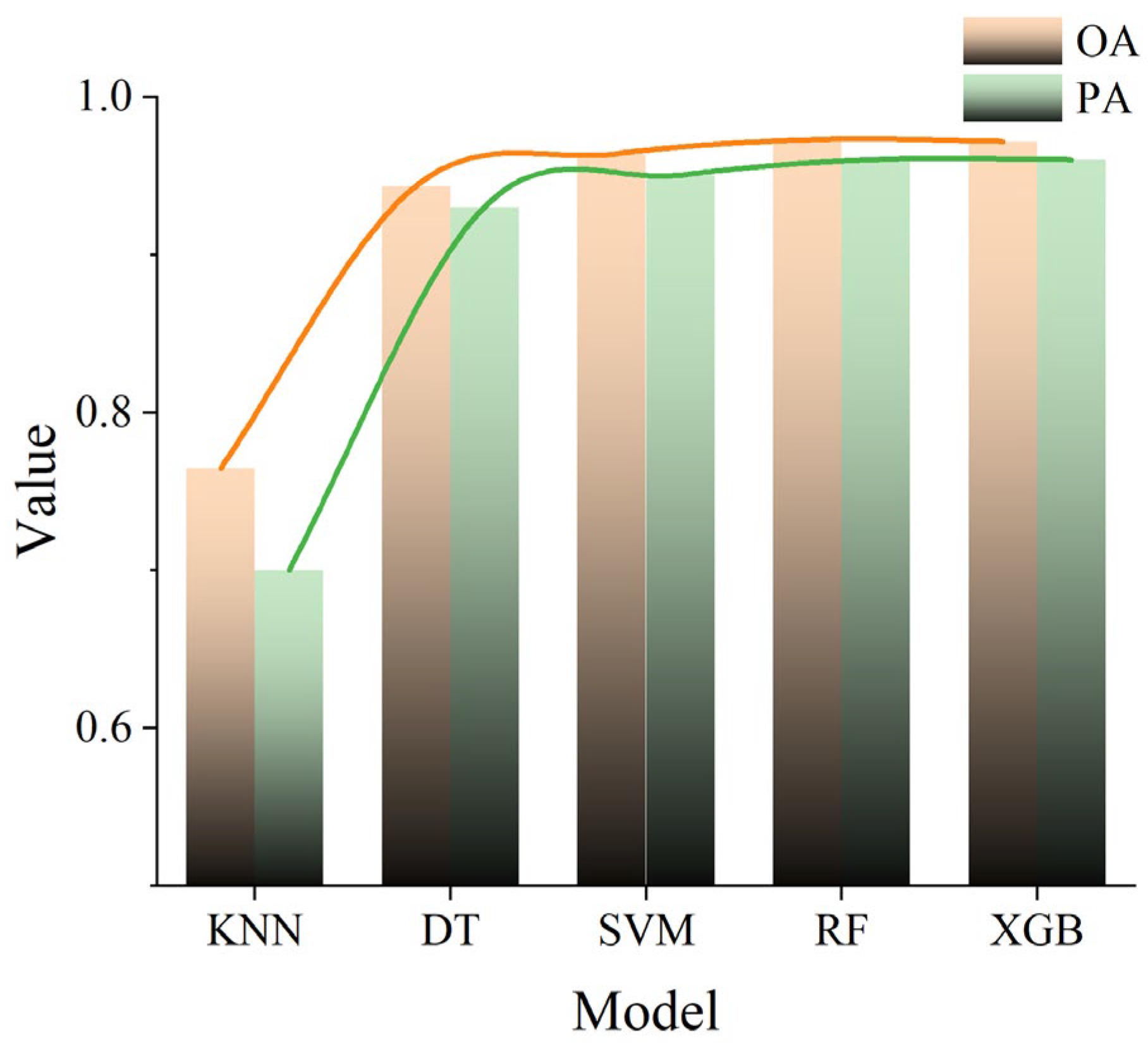
Among the models, RF demonstrates the best performance under the S5 scheme, achieving an OA of 97.24% and a Kappa coefficient of 0.96. Compared with the other models, the OA of RF exceeds that of KNN, DT, SVM, and XGBoost by 20.76%, 2.9%, 0.9%, and 0.07%, respectively. Its Kappa coefficient is also close to that of XGBoost but surpasses KNN, DT, and SVM by 0.26, 0.03, and 0.01, respectively. Aside from RF, DT, SVM, and XGBoost also achieve OA values above 90% and Kappa coefficients exceeding 0.9, indicating high accuracy and stability under the S5 scheme. Overall, RF exhibits the most pronounced advantage, SVM and XGBoost perform comparably, while KNN continues to show relatively limited classification performance (Figure 13).

4.4. Impervious Surface Extraction Results

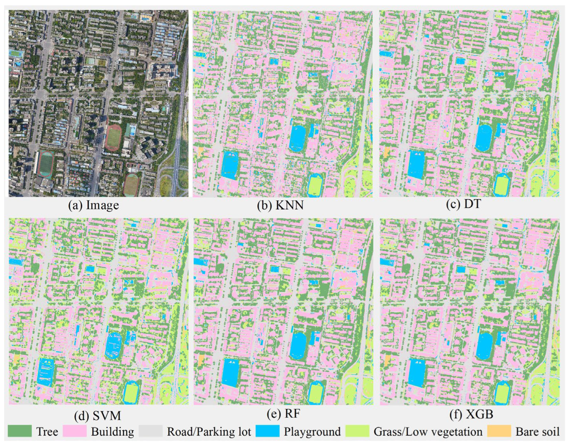
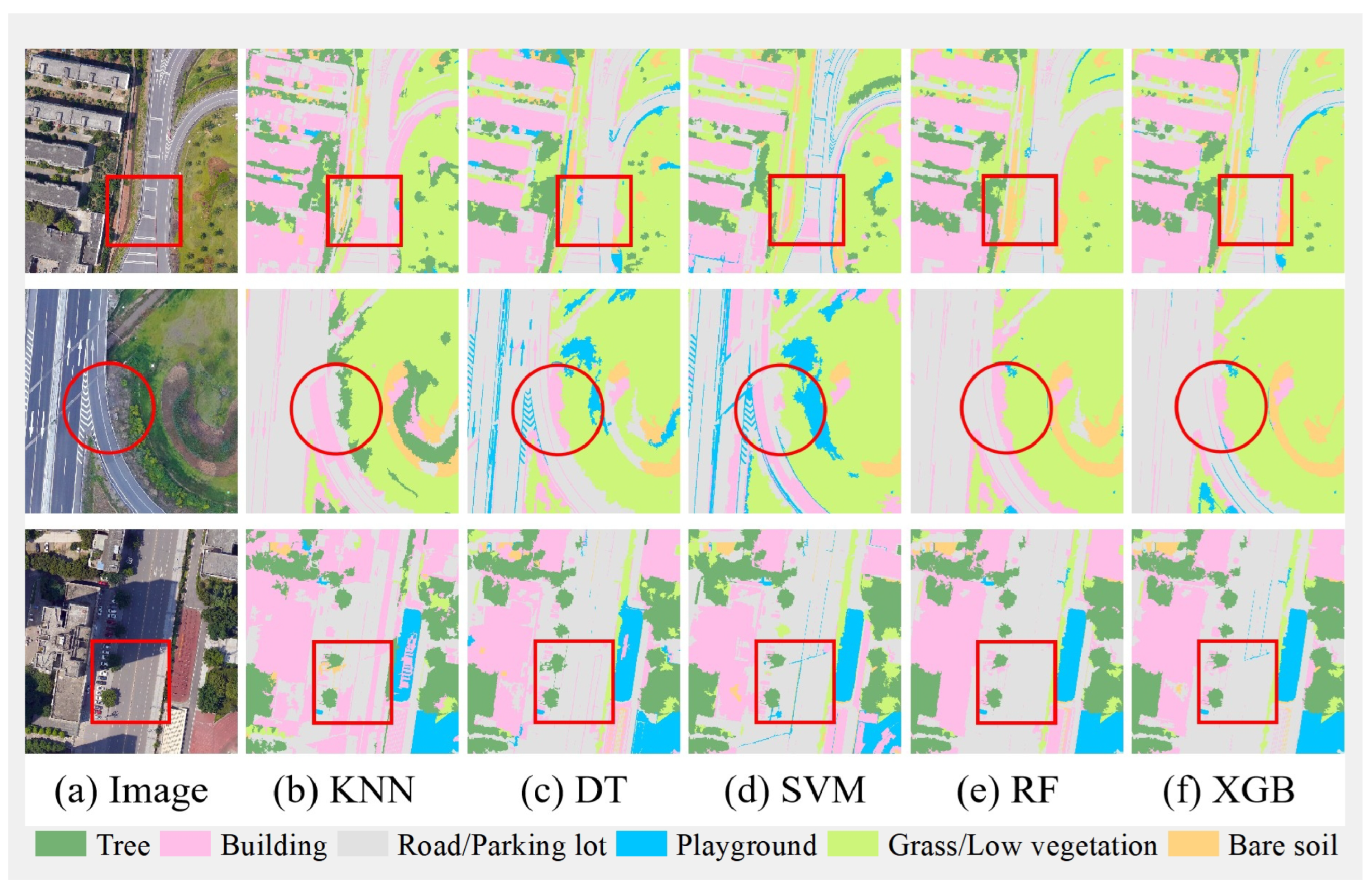
Under the optimized feature set scheme (S5), five classification models—KNN, DT, SVM, RF, and XGBoost—are applied to classify land cover in the study area, and the results are shown in Figure 14 and Figure 15. Overall, all models are able to distinguish the main land-cover types with reasonable accuracy, but clear differences are observed in classification precision, boundary delineation, and the recognition of small-scale objects.

Among models, RF demonstrates the best overall performance. In terms of boundary preservation, RF effectively delineates the contours of typical impervious surfaces such as roads and buildings, while achieving high accuracy in recognizing small-scale features such as narrow roads and scattered bare-soil patches. Its classification results align closely with the actual land-cover distribution, with few misclassifications, thereby avoiding confusion between roads and buildings. This indicates that RF, as an ensemble tree-based model, has strong nonlinear fitting capacity and robustness to noise, making it well suited for complex classification tasks under multi-source, high-dimensional feature conditions.

XGBoost and SVM follow in performance. Both achieve good boundary preservation and reliably distinguish major land-cover types, producing relatively coherent classification maps. However, localized errors remain: XGBoost exhibits confusion at some road–building boundaries, while SVM occasionally misclassifies sports fields and grasslands in mixed areas. Nevertheless, both models maintain high accuracy overall. These results suggest that SVM, with its margin maximization principle, and XGBoost, with its gradient boosting strategy, have clear advantages in handling high-dimensional features, though their performance declines in highly complex or spectrally mixed local environments. By contrast, KNN and DT perform less effectively in the heterogeneous urban setting. KNN, constrained by its distance-based mechanism, is prone to confusion among spectrally similar classes and occasionally misclassifies roads as buildings. DT, as a single-tree model, is highly sensitive to imbalanced sample distributions and shows instability, even misclassifying roads as sports fields in some areas, leading to blurred boundaries and reduced overall accuracy. These findings indicate that simple models are inadequate for fully exploiting the complex relationships among high-dimensional features, and their classification stability and boundary-preserving ability are inferior to ensemble models.

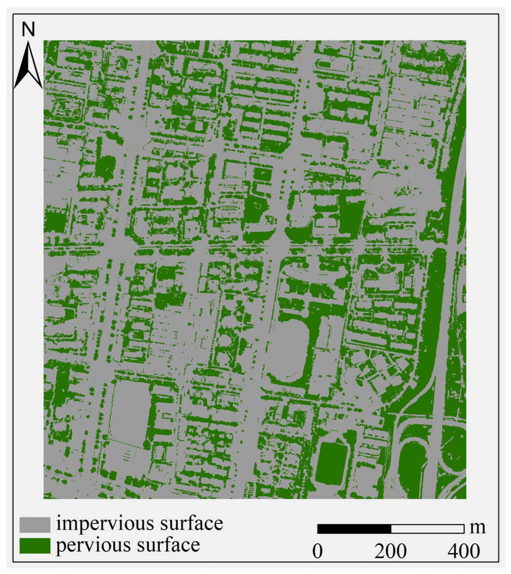
To achieve the objective of impervious surface extraction, the land-cover classification results obtained from the optimal scheme (S5-RF) were further reclassified to derive the final impervious surface areas (ISA). As shown in Figure 16, buildings and roads/parking lots were aggregated into a single ISA category, resulting in a fine-scale ISA map with clear spatial patterns and well-defined boundaries.

The incorporation of LiDAR-derived features plays a critical role in reducing spectral confusion with bare soil and vegetation, thereby improving class separability and producing more continuous and geometrically consistent impervious surfaces, which are essential for fine-scale urban impervious surface extraction.

5. Discussion

This study focuses on fine-scale urban impervious surface (ISA) extraction using multi-source UAV data, and the results highlight the importance of integrating spectral and structural information for improving classification performance in complex urban environments. Compared with previous studies based on high-resolution satellite imagery, UAV-based data provide centimeter-level spatial detail, which is particularly advantageous for representing small and heterogeneous urban features [41,42]. This finding is consistent with previous research demonstrating that increasing spatial resolution can effectively reduce mixed-pixel effects and improve ISA extraction [8,43].

The integration of UAV optical imagery and LiDAR data plays a critical role in addressing spectral confusion [13,16], which remains a major challenge in ISA extraction. Previous studies have shown that spectrally similar classes, such as roads, rooftops, and bare soil, are difficult to distinguish using optical data alone [44]. In this study, LiDAR-derived features—particularly the normalized digital surface model (NDSM)—provide essential height information that significantly enhances class separability. The high importance of NDSM observed in the SHAP analysis further confirms the dominant role of structural features in distinguishing impervious surfaces, which is consistent with findings reported in previous studies [45]. These results indicate that the integration of spectral and geometric information is a key factor in improving classification accuracy in complex urban environments [46].

At the segmentation level, the proposed EGS-Optimizer introduces a unified optimization framework that integrates edge detection with the global segmentation quality (GS) index. Unlike conventional ESP2-based methods that rely on visual interpretation [29], or GS-based approaches that only consider statistical homogeneity [27], the proposed method incorporates boundary information directly into the scale selection process. Qualitative comparisons indicate that the incorporation of edge constraints leads to more refined object boundaries. This suggests that the EGS-Optimizer provides a practical improvement for object-based segmentation, particularly in fine-scale urban scenarios where accurate boundary delineation is essential. In terms of feature representation, the SHAP-based feature selection strategy effectively reduces feature redundancy and enhances model interpretability. The results show that reducing the feature set from 45 to 21 variables not only decreases computational complexity but also improves classification performance. Furthermore, the introduction of the F1-score provides a more balanced evaluation under class imbalance conditions. The results indicate that the optimized feature set improves the classification performance of minority classes, such as bare soil, thereby enhancing the robustness of the model. These findings are consistent with recent studies, emphasizing the importance of feature selection in high-dimensional remote sensing data [47].The high overall accuracy (OA = 97.24%) achieved in this study must be contextualized within the historical progression of ISA extraction methodologies. Early studies relying on medium-resolution satellite imagery (e.g., Landsat or Sentinel data) typically reported accuracies ranging from 80% to 90% [48], constrained by mixed-pixel effects. The transition to spaceborne high-resolution imagery improved these accuracies, yet spectral confusion remained a persistent bottleneck [46]. The accuracy improvement observed in our framework is not merely a result of increased spatial resolution, but rather the synergistic integration of spectral and structural information. This aligns with recent findings that LiDAR-derived structural features, particularly NDSM, are critical for resolving spectral ambiguity in complex urban environments [45,49,50]. Furthermore, while deep learning methods (e.g., CNNs, U-Net) have demonstrated strong capabilities, their effectiveness typically depends on large annotated datasets and high computational costs [51,52]. It should be explicitly noted that the above comparison with deep learning represents a qualitative, conceptual discussion rather than an empirical benchmark, as direct numerical comparisons were not conducted in this study. Nevertheless, the traditional machine learning approach adopted here, combined with SHAP-based interpretability, provides a transparent and resource-efficient alternative that demonstrates highly competitive performance under limited sample conditions.

At the methodological level, this improvement is driven by two key optimizations. First, the proposed EGS-Optimizer addresses a practical challenge in OBIA. Unlike conventional ESP2 methods that rely on visual interpretation [29], or GS-based approaches that lack explicit boundary constraints [27], our framework embeds edge information directly into the segmentation feature space prior to scale selection, shifting edge detection from an auxiliary post-processing step to a primary input driver. This shifts edge detection from an auxiliary post-processing step to a core component of segmentation optimization, yielding measurably refined boundaries for fine-scale urban objects. Second, the reduction of the feature space from 45 to 21 dimensions via SHAP confirms that high-dimensional multi-source data inevitably introduces redundancy; targeted feature selection is essential for enhancing both computational efficiency and model robustness, particularly for minority classes like bare soil under imbalanced conditions [47]. UAV-based data provides the foundational centimeter-level spatial detail necessary to represent these heterogeneous features [13,44], but it is the optimized processing framework that translates this detail into classification accuracy.

A critical limitation of this study is the constrained spatial extent and the lack of cross-scene validation. While the high accuracy demonstrates the framework’s efficacy under controlled, fine-scale conditions, it does not inherently guarantee robustness in highly heterogeneous or large-scale urban environments. The study area, though representative of a typical inland basin city, exhibits relatively limited topographical and morphological complexity. Consequently, the proposed method’s ability to handle severe shadow interference, highly dense urban canyons, and extreme class imbalance—common challenges in megacities—remains unverified. Additionally, the reliance on UAV data inherently restricts spatial coverage and increases acquisition costs compared to satellite-based approaches, limiting the framework’s current applicability to large-area mapping tasks. From an application perspective, the proposed framework is particularly suitable for fine-scale urban analysis, such as neighborhood-level impervious surface mapping, urban micro-environment assessment, and stormwater management. Its ability to accurately delineate small urban objects provides valuable support for high-precision urban planning and environmental monitoring. However, its extension to large-scale or cross-regional applications requires further methodological validation and adaptation.

Overall, this study provides a practical and interpretable framework for integrating multi-source UAV data in fine-scale ISA extraction, while also highlighting the need for further research on scalability, generalization, and robustness under more complex urban conditions.

6. Conclusions

Accurate extraction of urban impervious surfaces is essential for urban planning, environmental monitoring, and sustainable urban development. With the rapid advancement of high-resolution UAV remote sensing technologies, new opportunities have emerged for fine-scale urban impervious surfaces mapping.

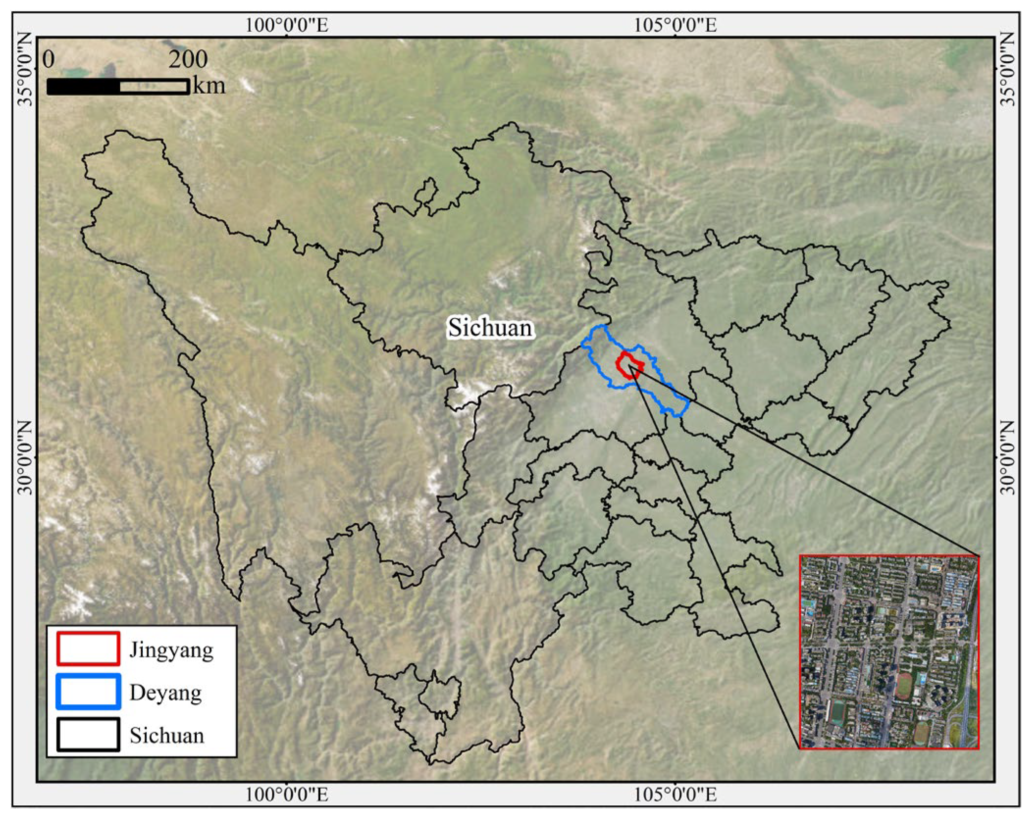
This study proposes a fine-scale urban impervious surface extraction framework by integrating UAV-LiDAR and high-resolution visible imagery. The framework incorporates an improved EGS-Optimizer, which combines edge detection with the global segmentation quality (GS) index for objective segmentation scale selection, as well as a SHAP-based feature selection strategy to reduce feature redundancy and enhance model interpretability. Experiments conducted in a representative urban area of Deyang, Sichuan Province demonstrate the effectiveness of the proposed approach in segmentation optimization, feature construction, and classification performance. The main conclusions are summarized as follows:

• The proposed EGS-Optimizer improves boundary delineation and enables more objective and quantitative determination of segmentation scales, providing a reliable basis for object-based analysis.
• The integration of UAV optical imagery and LiDAR data significantly enhances classification performance compared with single-source data, highlighting the importance of combining spectral and structural information in complex urban environments.
• The SHAP-based feature selection strategy effectively reduces feature redundancy (from 45 to 21 features) while improving model performance and interpretability. Among all features, the LiDAR-derived NDSM plays a dominant role in distinguishing impervious surfaces.
• Under the optimized feature set, the RF model achieves the best performance (OA = 97.24%, Kappa = 0.96), demonstrating the effectiveness of the proposed framework under fine-scale conditions.

It should be noted that the study is conducted in a relatively small and homogeneous urban area, and no cross-area or multi-scene validation is performed. Therefore, the findings primarily demonstrate the effectiveness of the proposed method for fine-scale urban analysis, rather than its general applicability to large-scale or heterogeneous environments.

Overall, the proposed framework provides an effective and interpretable solution for fine-scale urban impervious surface extraction using multi-source UAV data. The results support detailed ISA mapping at the neighborhood scale and provide useful insights for applications such as urban micro-environment analysis, stormwater management, and fine-scale urban planning. Future research should focus on extending the method to larger spatial scales, incorporating multi-source data such as SAR, and exploring deep learning-based approaches to further improve generalization and automation capabilities.