Skip to Content
Remote SensingRemote Sensing
  • Article
  • Open Access

21 April 2026

An Explainable Machine Learning Framework for Flood Damage Mapping Using Remote Sensing and Ground-Based Data: Application to the Basilicata Ionian Coast (Italy)


,
,
and
1
Department for Humanistic, Scientific, and Social Innovation, University of Basilicata, 75100 Matera, Italy
2
Department of Engineering, University of Basilicata, 85100 Potenza, Italy
*
Author to whom correspondence should be addressed.

Highlights

What are the main findings?
  • Flood damage susceptibility is mainly influenced by Drainage density (17.10%), Railway distance (16.33%), and Elevation (15.42%), while extreme precipitation (Max rainfall, 10.66%) and Street distance (7.51%) also play a relevant role. Socio-economic and other environmental factors, such as population density, elderly population, education level, and pedology, contribute less than 4% each.
  • Observed flood damage exhibits threshold-like behavior, while hydraulically modeled scenarios (return periods 30, 200, and 500 years) show continuous and progressively contracting gradients with increasing event severity.
What are the implications of the main findings?
  • Damage-based susceptibility mapping complements hydraulic hazard maps by identifying where inundation is more likely to translate into actual damage.
  • Threshold-related predictors provide quantitative support for prioritizing infrastructure protection and land-use regulation in flood-prone areas.

Abstract

Flood damage assessment remains challenging, as conventional flood risk management mainly relies on hydraulic hazard maps that do not explicitly reproduce observed damage patterns. Recent advances in remote sensing and machine learning (ML) enable the integration of environmental and socio-economic data with historical impact information to improve flood damage modeling. This study proposes an explainable machine learning framework for flood damage susceptibility mapping, using observed institutional damage records from the 2011 and 2013 flood events combined with 17 geospatial flood risk factors (FRFs) representing hazard, exposure, and vulnerability. This approach enables the capture of non-linear relationships between flood damage and FRFs. For comparison purposes, the same framework was also applied using hydraulically modeled flood extents corresponding to return periods of 30, 200, and 500 years. The framework was tested along the Basilicata Ionian coast in southern Italy, a Mediterranean region characterized by complex geomorphology, intense rainfall events, and recurrent flood impacts. An eXtreme Gradient Boosting (XGBoost) model was trained using 17 FRFs related to hazard, exposure, and vulnerability at a spatial resolution of 20 m. The model achieved high performance with an accuracy of 0.988, an F1-score for the minority class of 0.860, and an ROC-AUC (test) of 0.996. High to very high flood damage probability was predicted in approximately 4.1% of the study area, mainly in low-lying floodplains near river corridors and infrastructure. SHAP-based explainability analysis revealed that damage susceptibility was predominantly driven by hazard and exposure factors: Drainage density (17.10%), Railway distance (16.33%), and Elevation (15.42%), extreme precipitation (Max rainfall, 10.66%) and Street distance (7.51%), with socio-economic vulnerability contributing less than 4%. The observed damage target exhibited clear threshold-like patterns (e.g., sharp risk increases below ~25/35 m elevation or within ~150/200 m of road infrastructure), contrasting with the smoother, continuous gradients produced by hydraulic scenarios. This analysis identified the most influential predictors and their response ranges. The proposed framework complements hydraulic hazard mapping by explicitly modeling observed flood damage, supporting flood risk assessment in flood-prone coastal regions.

1. Introduction

Floods are defined as the temporary covering by water of land that is not normally inundated [1]. They are among the most damaging natural hazards, affecting populations worldwide each year [2]. According to the Centre for Research on the Epidemiology of Disasters (CRED) EM-DAT database (https://www.emdat.be, accessed on 5 February 2025), floods affected approximately 1.88 billion people globally between 2000 and 2025, representing about 39% of all people affected by natural disasters during this period. Floods are also responsible for severe damage to infrastructure and the environment [3,4]. Globally, floods caused average annual socioeconomic losses of more than USD 2.5 billion from 1960 to 2017, while in Europe, flood-related economic damages totaled about EUR 385.7 billion between 1980 and 2024 [5]. Over recent decades, both the frequency and intensity of floods have increased due to the combined effects of climate change, rapid population growth, and urbanization [6,7]. As a result, flood risk is expected to increase globally over time, whereby flood risk can be understood as the combination of the probability of a flood event and its potential adverse consequences for human health, the environment, cultural heritage, and economic activity [1].
With the increasing frequency and intensity of floods worldwide, effective flood risk mitigation has become increasingly critical [8]. In response, the European Union adopted the EU Floods Directive [1], which establishes a comprehensive framework for flood risk management, including flood risk assessment, the preparation of flood hazard and flood risk maps, and the development of flood risk management plans at the river basin scale [1]. This directive marked a transition from traditional flood management toward a risk-based approach in Europe, emphasizing the joint use of flood hazard and flood risk maps to represent not only the probability of flood events but also their potential impacts, such as economic losses and the number of affected people [9]. Many studies regarding to the flood hazard mapping have been carried out [10,11,12,13,14]. However, hazard maps cannot explicitly reproduce observed damage patterns [15]. Hence, in recent years, many studies have emphasized the need for an integrated assessment approach that goes beyond physical dimensions of hazard and exposure to also incorporate social dimensions of vulnerability for flood risk management [8,9,15,16]. Flood hazard is first characterized in terms of the probability and intensity of inundation events. Exposure and vulnerability are then combined with hazard information to estimate potential adverse consequences, including economic damages and impacts on population, using flood damage models. Finally, flood risk is quantified by integrating these potential consequences across flood events with different probabilities or return periods [17].
Based on previous studies, several approaches have been used to assess flood risk, including: (i) statistical methods [18,19], (ii) multi-criteria analysis [20,21], (iii) Geographic Information System (GIS) and Remote Sensing (RS)-based analysis [22,23,24], and (iv) scenario-based inundation analysis [9,25,26]. Recent advances in RS and GIS, combined with machine learning (ML), have enabled multidisciplinary approaches for improved flood mapping, monitoring, and management [8,27]. RS and GIS techniques play an important role in flood mapping and monitoring [3,8], and their integration with ML has been shown to improve predictive accuracy, reduce computational time, and lower model development costs [8]. Various ML algorithms have been applied to support flood risk assessment and damage mapping, including classification models and ensemble learning methods [8,27,28,29]. Among these, tree-based ensemble models such as Random Forest (RF), eXtreme Gradient Boosting (XGBoost), and Adaptive Boosting (AdaBoost) represent the current state-of-the-art. These models improve predictive performance by reducing variance and bias, increasing accuracy, and enhancing robustness to noisy and complex datasets [29]. In addition, there is growing interest in explainable artificial intelligence (XAI) techniques, such as SHAP (SHapley Additive exPlanations), which are integrated into ML models to interpret their outputs and provide greater transparency and interpretability of the results [30,31]. The combination of tree-based ML models and XAI techniques improves not only predictive performance but also the transparency and reliability of flood risk assessments [31].
Recent studies on flood in Italy have increasingly applied machine learning (ML) techniques for susceptibility mapping [7,10,14,32]. For example, deep neural networks have been used to rapidly delineate flood-prone areas [10], while hybrid ensemble models have been applied to assess flash flood susceptibility [32]. In addition, ML approaches have been used for flood forecasting [14], and their integration with GIS and remote sensing has improved the accuracy and effectiveness of flood hazard assessment and mapping [7]. In contrast, flood damage mapping studies in Italy have been primarily based on statistical methods and scenario-based approaches [25,26,33,34]. However, limited attention has been given to the combined use of historical flood damage records and a comprehensive set of flood risk factors (FRFs), including both physical and socio-economic variables, within advanced ML frameworks for flood damage modeling. Furthermore, integrating XAI such as SHAP can enhance model interpretability by quantifying the contribution and relative importance of each FRF to flood damage.
In Italy, particularly southern regions like Basilicata, hydro-geological instability exacerbates flood risks due to complex geomorphology, lithological heterogeneity, and intense rainfall [35]. The Ionian coast, encompassing basins like Bradano, Basento, and Cavone, has experienced recurrent floods over two centuries, causing severe economic, environmental, and human losses [36,37]. Recent events, such as those in 2011 and 2013, highlight vulnerabilities in low-lying plains and urban areas [37].
Given the persistence and intensity of flood events in the area, there is a need for approaches that combine observed damage data with quantitative information on terrain and infrastructure. This study aims to address this need by developing a data-driven machine learning framework to assess and map flood damage along the Ionian coast of Basilicata. The analysis of historical records shows a clear temporal and spatial concentration of damage, mainly along the middle and lower reaches of the Bradano and Basento basins. These patterns highlight the role of geomorphology, land use, and rainfall intensity in influencing the distribution of flood damage. The proposed approach combines institutional damage records with geospatial predictors to identify areas where physical and human factors increase flood susceptibility. The resulting maps provide useful information for basin planning, risk management, and civil protection at the regional scale.
This study addresses these gaps by posing the following research questions:
  • Can an XGBoost model, trained on remote sensing and institutional data, provide replicable maps for mitigation?
  • What are the dominant geospatial factors driving flood damage mapping in the Basilicata Ionian coast?
  • How do critical thresholds in these factors influence flood damage mapping?
  • What is the added value of satellite-derived data compared with conventional flood hazard maps?
To answer these questions, the XGBoost model was applied using historical flood damage records as the target variable and 17 flood risk factors (FRFs) as predictors.
SHapley Additive exPlanations (SHAP) analysis was then employed to quantify the relative importance of all predictors and highlight the most influential features, and Partial Dependence Plots (PDP) were subsequently applied to these key features to determine meaningful operational thresholds, illustrating how each factor affects the predicted probability of flood damage.

2. Materials and Methods

2.1. Case Study

The study area is located along the Ionian coastline of the Basilicata region, in Southern Italy, extending and partially involving adjacent territories of Calabria and Apulia (Figure 1). This coastal sector represents one of the most geomorphologically and hydrologically complex areas of the Southern Apennines, characterized by low-gradient alluvial plains, coastal dunes, reclaimed agricultural lands, and river mouths subject to strong fluvial–marine interactions. The area includes the lower courses and coastal outlets of several relevant river systems, mainly belonging to the Bradano, Sinni, and regional Basilicata hydrographic units, which drain large inland catchments towards the Ionian Sea.
Figure 1. Location of the Ionian coastline in the Basilicata region.
These river basins are prone to recurrent flooding, exacerbated by intense rainfall events, sediment transport dynamics, land-use changes, and progressive coastal modification. Urban settlements, touristic infrastructures, and highly productive agricultural areas are extensively distributed within flood-prone zones, leading to a high exposure to hydraulic risk. Throughout the twentieth century, multiple severe events were registered, particularly in the Ionian basins of Bradano and Basento. Between 1921 and 2014, forty-eight major flood events were documented, thirteen of which caused fatalities and extensive material losses [38]. The 1925 flood produced 340 mm of rainfall in Lauria over two days, while the 1946 event delivered more than 300 mm at Bernalda and Pomarico, inundating the Metaponto plain. The 1959 flood remains one of the most devastating episodes: 314.6 mm were recorded at Pisticci, 80 mm in one hour at Policoro, and 87 mm at Nova Siri, leading to the inundation of entire agricultural zones, collapse of infrastructure, and eleven deaths. During the 1970s, repeated high-intensity storms caused significant damage to the settlements of Pisticci, Craco, and Montalbano Jonico, where landslides affected residential areas. The 1990s again witnessed major floods in the Metaponto region, with the 1990 and 1996 events inundating large tracts of farmland and interrupting transport lines.
In recent decades, the March 2011 and October–December 2013 floods have been the most impactful, causing both human and economic losses. In March 2011, rainfall exceeded 150 mm in 24 h between Ferrandina, Grottole, and Tursi, leading to widespread inundation and the evacuation of more than 200 families. The October 2013 storm delivered 189 mm in 12 h at Bernalda (Torre Accio) and 121 mm in Scanzano Jonico, resulting in the overflow of the Bradano and Basento rivers and several casualties near Ginosa. The December 2013 event, with cumulative rainfall above 200 mm at Metaponto and 157 mm at Matera, triggered further flooding, infrastructure failures, and the large Montescaglioso landslide with vertical displacement of up to 10 m. These events produced extensive damage to transport networks, agricultural areas, and residential settlements, requiring large-scale emergency and recovery interventions. The investigated basin is characterized by extensive low-elevation floodplains, limited hydraulic conveyance capacity, and growing anthropogenic pressure linked to land-use changes, all of which contribute to heightened flood susceptibility.

2.2. Multi-Source Dataset

2.2.1. Flood Inventory Maps

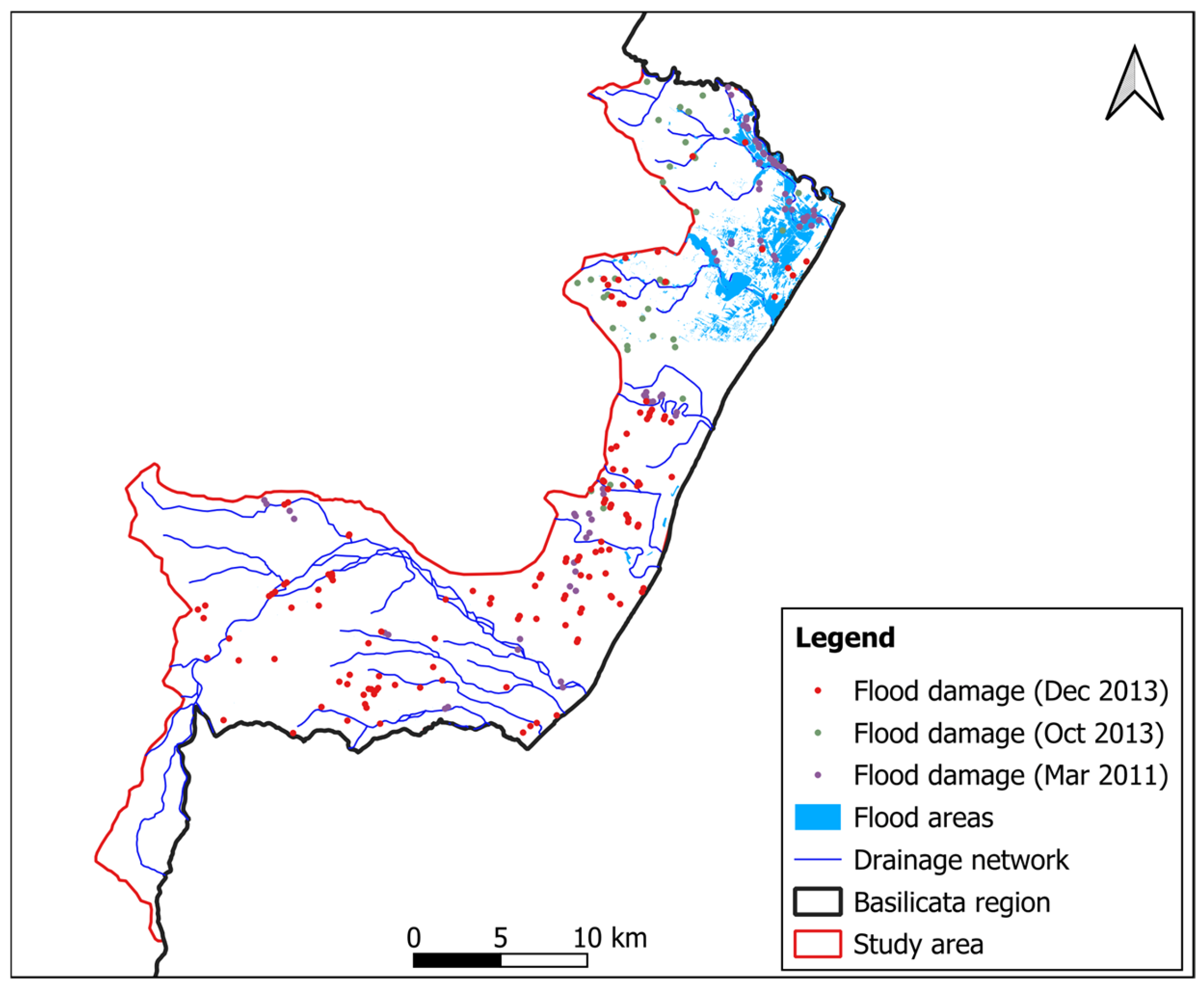
A detailed flood inventory for the Basilicata River basin was developed by collecting, and harmonizing information on historically flooded areas from multiple institutional sources, including datasets provided by the Basilicata Regional Authority, and the University of Basilicata. Historical documentation and satellite-based analyses have highlighted several major flood events affecting the study area, notably those that occurred in March 2011, October 2013, and December 2013. The satellite images used to delineate the observed flood extents primarily cover the Metaponto coastal plain, extending for approximately 40 km along the central Ionian coastline of Basilicata and including the lower reaches and coastal outlets of the Bradano and Basento rivers (Figure 2). Flood extent information was derived from products available through the Copernicus Emergency Management Service (EMS) and from COS-MO-SkyMed (CSK) imagery supplied by the Italian Space Agency (ASI) following re-quests from the National Civil Protection Department. CSK acquisitions were obtained in Stripmap mode, with a spatial resolution of 2.5 m and both horizontal and vertical polarization configurations. Further technical details on the analyzed events and satellite datasets can be found in the recent literature [26,37]. Specifically, the following datasets were used:
Figure 2. Observed flood areas and local damages in March 2011, October and December in 2013.
  • March 2011 flood event: Multispectral COSMO-SkyMed imagery covering the flooded areas was georeferenced and processed using a semi-automated supervised classification approach to delineate inundated pixels.
  • October 2013 flood event: Flood extent maps were retrieved from the Copernicus EMS, based on SPOT-6 acquisitions dated 17 October 2013 at 11:40 a.m.
  • December 2013 flood event: Flood mapping products for the Basilicata Ionian coast were derived from satellite acquisitions conducted on 2–3 December 2013 at 4:31 a.m. Additional Copernicus EMS data from 4 and 5 December (10:55 a.m. and 12:55 p.m.) were integrated to reconstruct the temporal evolution of inundation processes.

2.2.2. Database of Damage Forms

The core dataset used in this study was derived from institutional archives documenting verified hydraulic damages in the Basilicata Ionian coastal sector. Two official sources were integrated to represent confirmed damage occurrences: (i) a regional database of hydraulic criticalities, and (ii) the damage records derive from nationally standardized post-emergency assessment forms, used within the Italian Civil Protection system to quantify structural and economic losses following the declaration of a state of emergency. These forms provide spatially explicit information on the typology and location of damages affecting residential, industrial, agricultural, and infrastructural assets. The overall dataset comprises 276 validated post-event records related to the March 2011, October 2013, and December 2013 flood events (94, 46, and 136 records, respectively), which constitute the empirical basis for model training, validation, and susceptibility mapping (Figure 2). The positive class (damage = 1) was assigned to the 20-m raster cells containing the geographic coordinates of the 276 validated institutional damage records (no buffer applied). All remaining pixels within the study area were labeled as no damage (class 0).
It should be noted that, for the coastal area considered, the available records are relatively limited compared to the overall extent of the study area, with large portions lacking recorded damage. This aspect is addressed in greater detail in the Section 2.4, where the procedures adopted for dataset preparation for model training and for handling the presence and absence damage classes (1 and 0, respectively) are described.

2.2.3. Flood Hazard Zoning

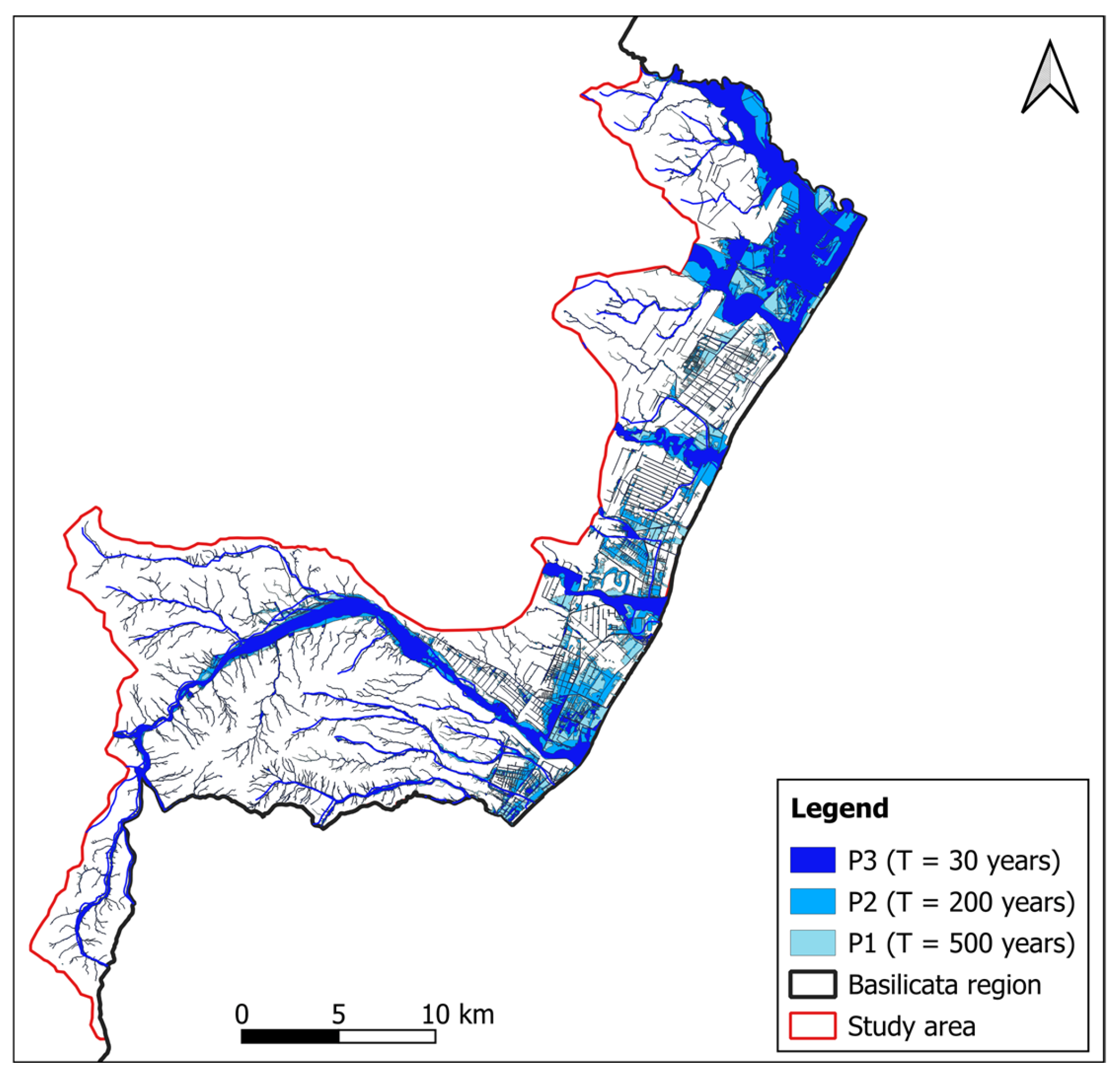
In October 2024, the Southern Apennines District Basin Authority adopted the current delineation and classification of floodplain areas within the Hydrogeological Risk Management Plan (PAI—River Bands and Hillslope Areas) for the Lucanian Ionian Coast. This framework is based on detailed hydraulic analyses and an enhanced knowledge base derived from Flood Risk Management Plans (PGRA), developed in accordance with the EU Floods Directive [1]. The floodplain mapping defines hydraulically hazardous areas classified into high (P3), medium (P2), and low (P1) flood hazard levels. The delineation provides a spatially consistent representation of flood-prone zones, with particular detail in coastal sectors and river mouths, where flood dynamics are strongly affected by backwater conditions and coastal processes. These areas are subject to safeguard measures that are immediately binding within the planning framework. The adopted flood hazard zoning constitutes the authoritative institutional reference for flood risk assessment and territorial planning along the Ionian coastal area. In this study, it is used as the regulatory baseline against which observed flood damage patterns and machine-learning-based damage susceptibility maps are evaluated, ensuring coherence with current planning and risk management instruments.
The floodplain maps used for validation purposes are shown in Figure 3.
Figure 3. Overview of the four damage maps considered in this study: and officially delineated maps P1 (500-year return period), P2 (200-year return period), and P3 (30-year return period).

2.3. Flood Risk Factors

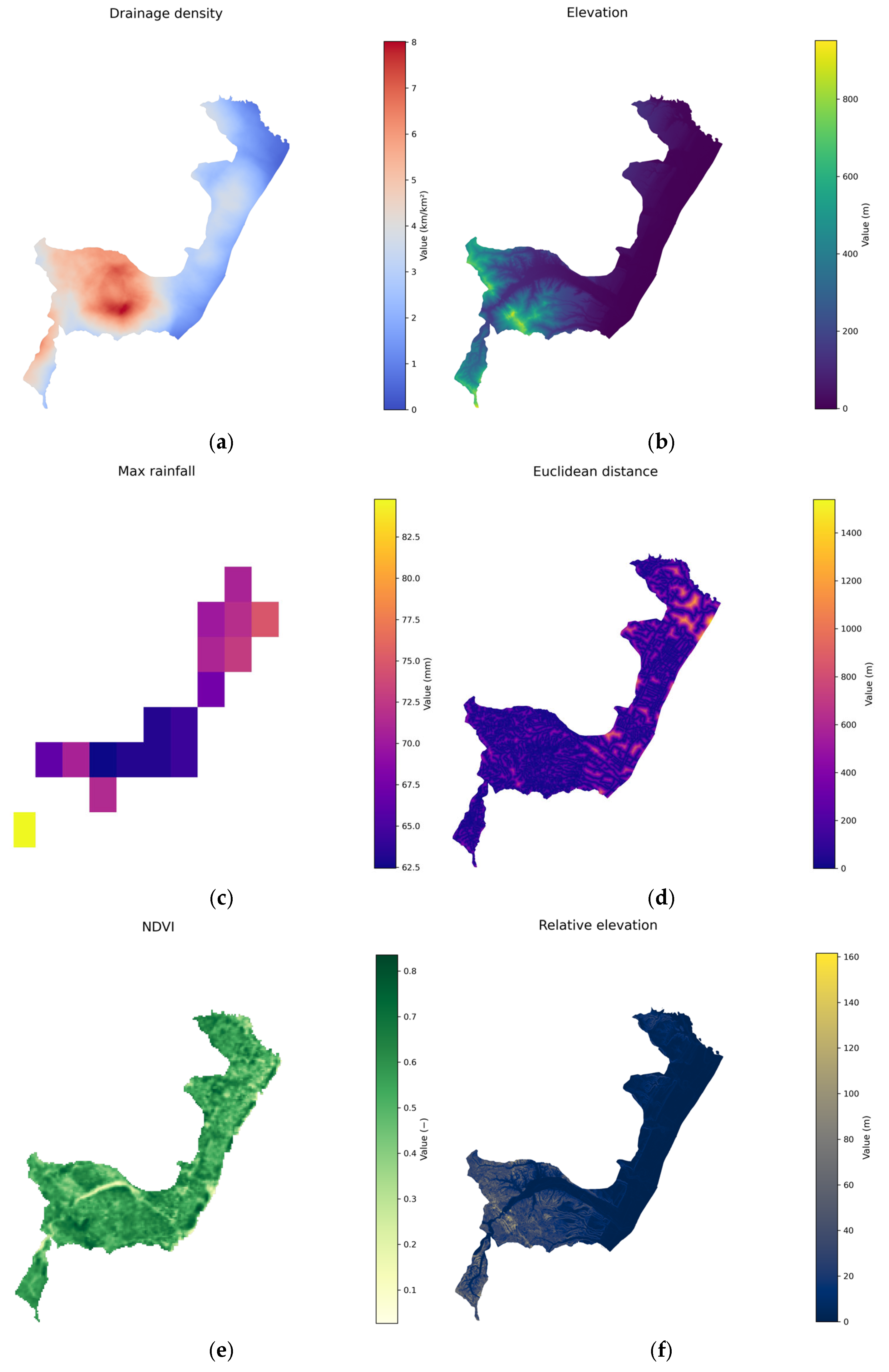
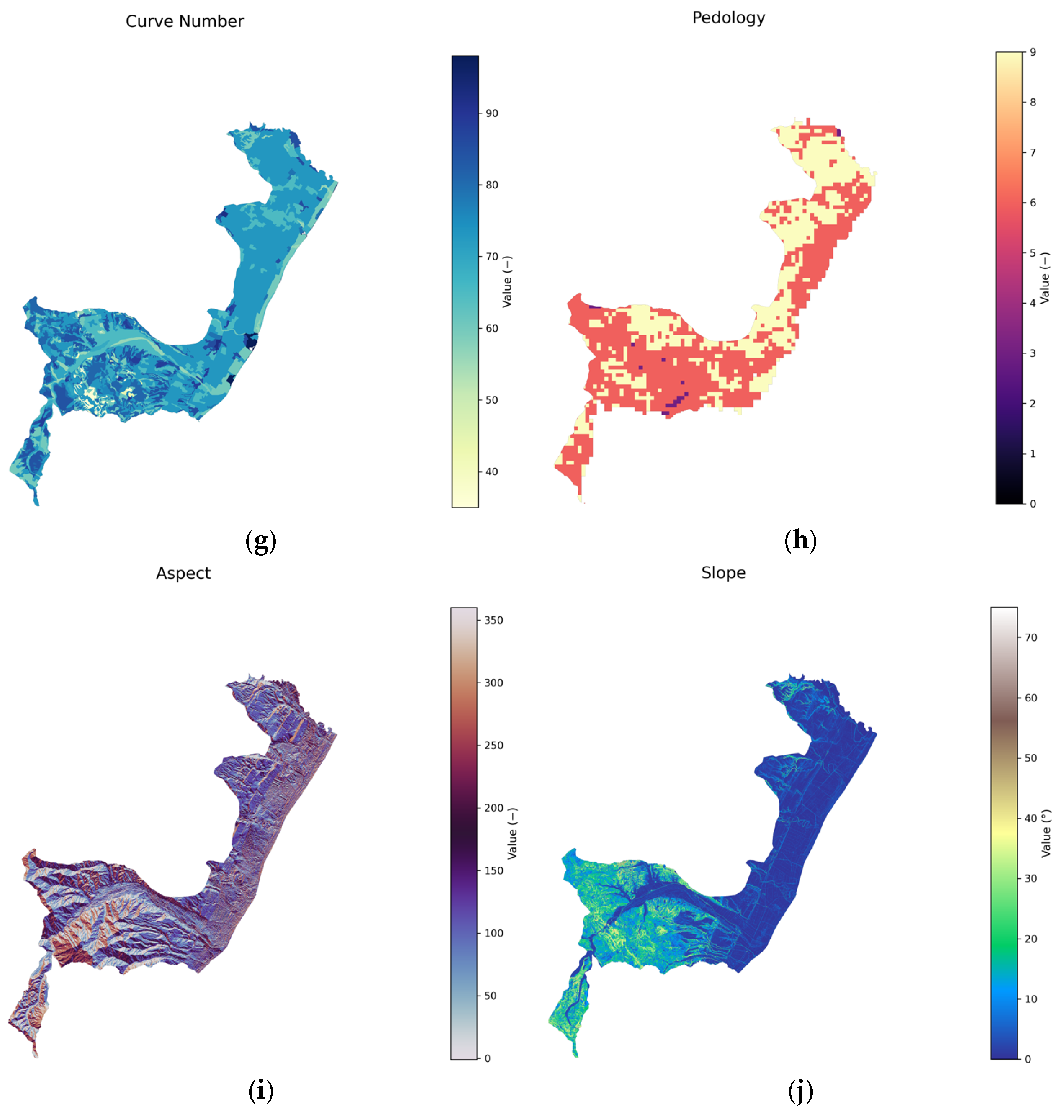
The environmental and anthropogenic conditions of each cell were described by 17 flood risk factors, which represent the main predisposing factors of hydraulic instability. These predictors were categorized into three groups based on flood risk components: hazard (physical and environmental factors contributing to flood occurrence), exposure (elements at risk, such as infrastructure and population), and vulnerability (socioeconomic factors affecting resilience and recovery). All the predictor layers were projected to a common coordinate reference system WGS84 and resampled to a 20 m spatial resolution, enabling their integration within the machine learning framework for flood damage mapping.
Topographic and hydrological predictors were derived from the official geospatial datasets of the Basilicata Region. Elevation data were obtained from airborne LiDAR surveys and photogrammetric processing and provided as a Digital Terrain Model (DTM).
Slope values were computed for each raster cell using a 3 × 3 cell moving window and the planar method, which estimates the maximum rate of elevation change between neighboring cells.
Aspect was computed using the same planar approach and describes the orientation of the steepest slope gradient. Aspect values were classified into eight cardinal directions (N, NE, E, SE, S, SW, W, NW).
Relative elevation was calculated to represent the vertical distance between each pixel and the nearest drainage channel, capturing local topographic controls on flood propagation. This parameter was obtained by subtracting the base-level elevation associated with the closest river or stream from the surface elevation of each pixel.
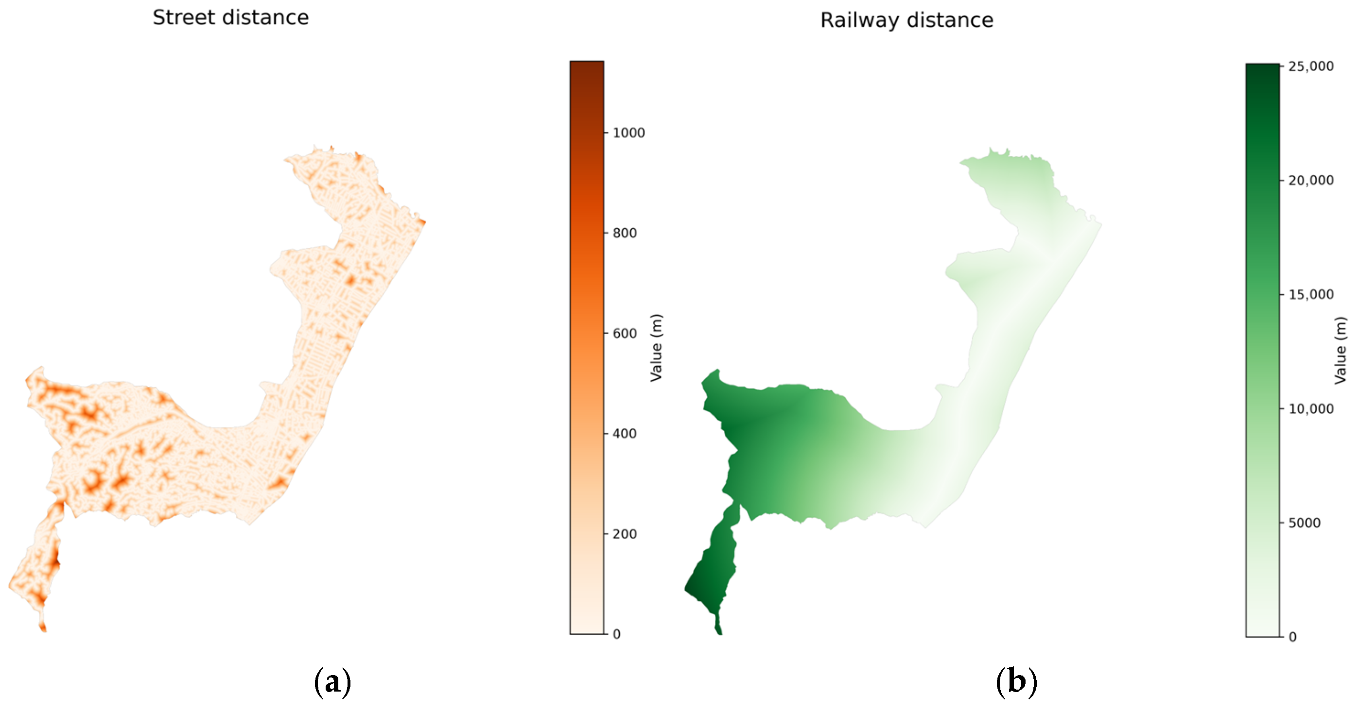
Distance to the hydrographic network was computed using a GIS-based Euclidean distance analysis, assigning each pixel the shortest horizontal distance to the nearest drainage feature. In addition, a flow-path distance approach was implemented to better represent hydraulic connectivity by simulating realistic runoff pathways between terrain elements and the drainage system.
Drainage density was estimated by dividing the total length of stream segments within a predefined grid cell by the cell area, using a moving-window analysis. Areas characterized by high drainage density correspond to well-developed fluvial networks and are typically associated with enhanced surface runoff and increased flood susceptibility.
Maximum precipitation intensity was derived from the Climate Hazards Center Infrared Precipitation with Stations (CHIRPS) version 3 at its native 0.05° resolution. This dataset combines satellite-based thermal infrared rainfall estimates with in-situ station observations to produce a 0.05° gridded rainfall time series over land. CHIRPS rainfall data have been widely used in flood risk mapping studies [39,40,41]. The reanalysis dataset is available from https://data.chc.ucsb.edu/products/CHIRPS/v3.0/ (accessed on 10 February 2026). Subsequently, the data are resampled to the common analysis grid (20 m) based on the nearest-neighbor interpolation method. We acknowledge that this substantial downscaling ratio (~250) results in spatially uniform rainfall values across all pixels falling within each original CHIRPS grid cell (approximately 25 km2). Consequently, the maximum rainfall predictor primarily captures differences at the sub-regional scale rather than fine-scale spatial variability within the study area. In addition, only a limited number of rain-gauge stations with reliable records were available during the 2011–2013 events, further constraining the representation of local rainfall variability.
Vegetation conditions were characterized using the Normalized Difference Vegetation Index (NDVI), derived from the Terra Moderate Resolution Imaging Spectroradiometer (MODIS) (Santa Barbara Remote Sensing, Goleta, CA, USA) Vegetation Indices (MOD13Q1) version 6.1 data, which are generated every 16 days at 250-m spatial resolution [42]. MODIS NDVI has been widely used in flood detection and mapping in previous studies and those proved its reliability and performance [43,44]. NDVI data was chosen for pre-event conditions because it reflects baseline vegetation conditions prior to flooding. The data are resampled to a 20-m grid based on the nearest-neighbor interpolation method.
Soil and land use properties were integrated through the Curve Number parameter, representing the combined effects of soil permeability, land use, and antecedent moisture conditions on surface runoff generation. Curve Number values were assigned using soil and land-use maps and resampled to the common analysis grid.
Pedological information, including soil texture, permeability, and lithological characteristics, was obtained from the regional pedological map and used to further refine infiltration-related hazard components.
Land-use data were obtained from the Regional Spatial Data Infrastructure (RSDI Basilicata), based on the CORINE Land Cover 2012 classification at a scale of 1:100,000. The dataset includes 44 land-cover classes organized into three hierarchical levels and provides essential information for both hazard and exposure characterization.
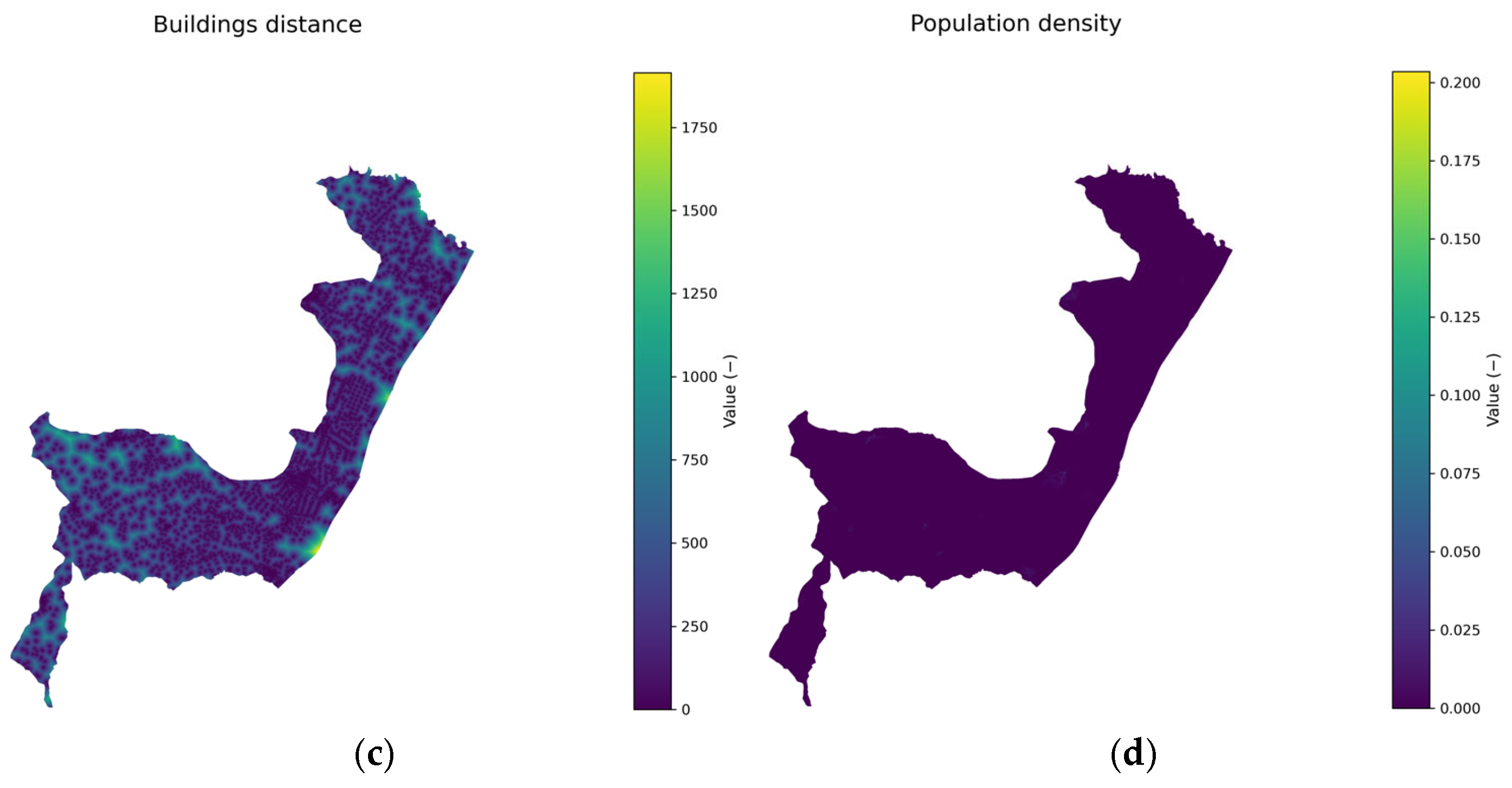
Exposure-related predictors were derived from regional geotopographic and transport datasets provided by the RSDI. Euclidean distance maps were generated for the road network, railway infrastructure, and built-up areas, representing proximity to exposed elements and critical infrastructure. Population density data, expressed as the number of inhabitants per square kilometer, were obtained from national census statistics provided by ISTAT and spatially distributed over the study area.
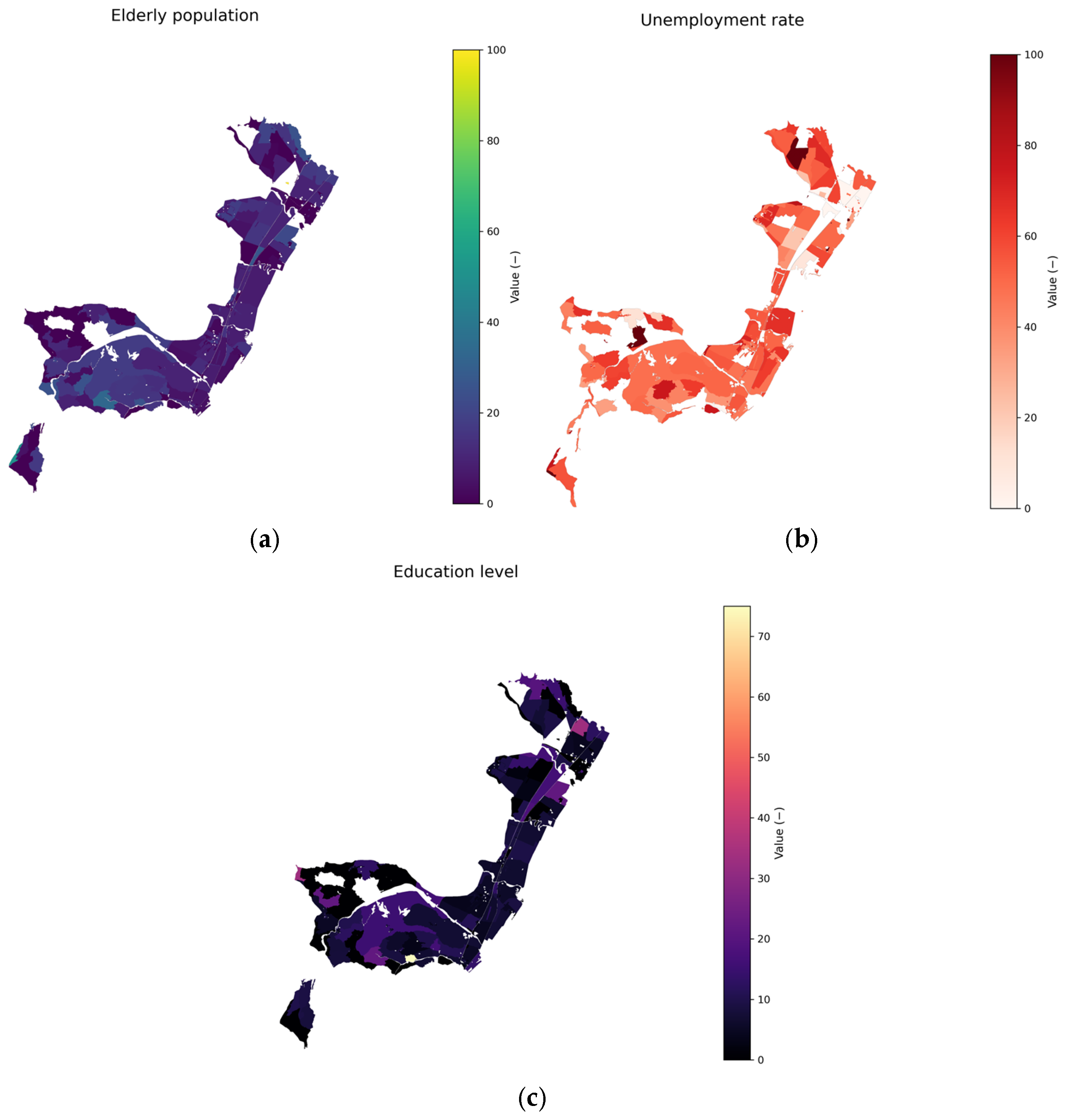
Vulnerability indicators were derived from socio-demographic census data provided by ISTAT, including the percentage of elderly population, the unemployment rate, and the average level of educational attainment.
The name of each factor, its short description and source can be found in Table 1 and the corresponding figures are provided in Appendix A.
Table 1. Sources and characteristics of the spatial data used in this study.

2.4. Conceptual Framework

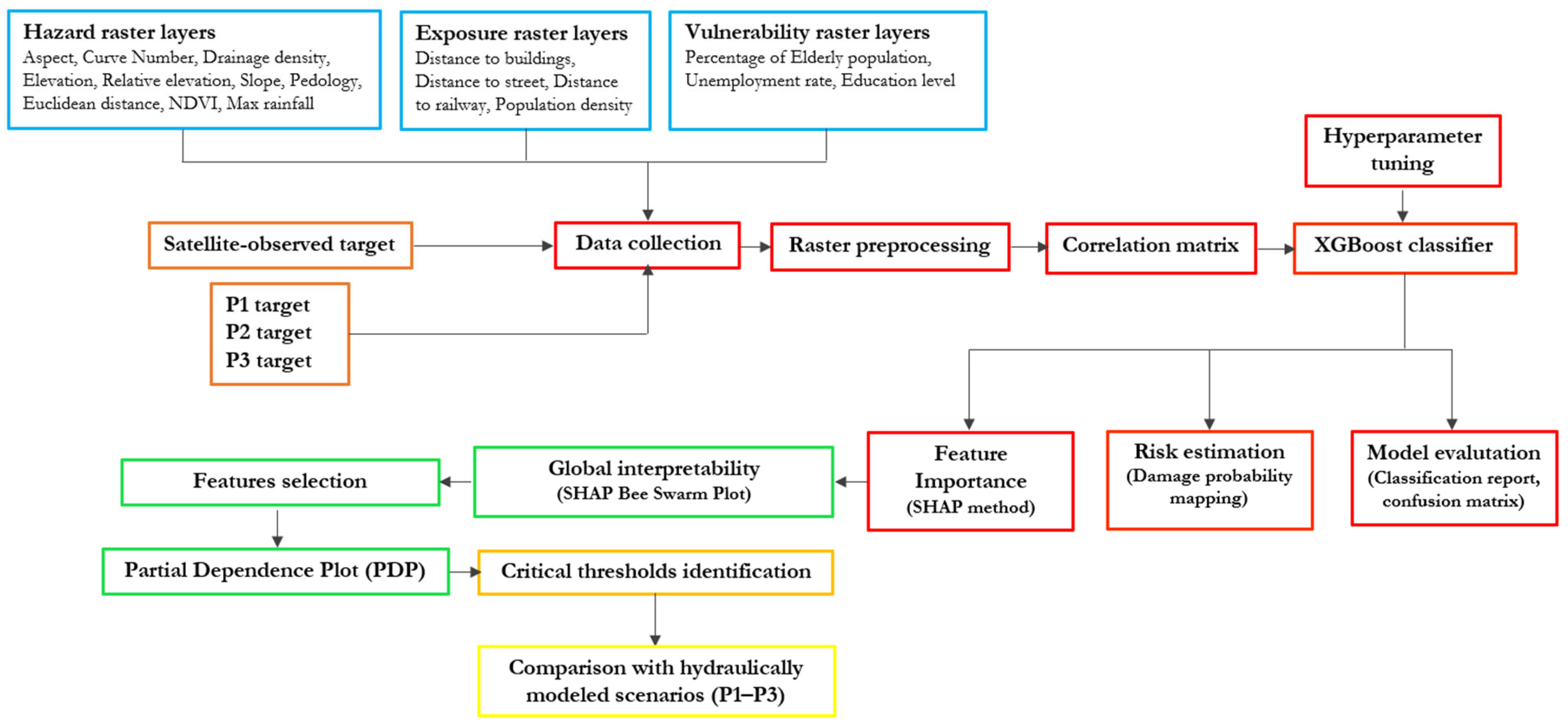
The methodological framework (Figure 4) was designed to identify and map areas susceptible to hydraulic failures across the Ionian coastline in the Basilicata region by combining verified institutional evidence of damage with geospatial predictors representing the physical and anthropogenic characteristics of the territory. To achieve this, eXtreme Gradient Boosting (XGBoost), which is a supervised machine learning model [45], was employed while the SHAP (SHapley Additive exPlanations) method was used to evaluate the influence of individual predictors on risk estimates and to interpret the model results. The approach integrates two complementary components: (i) an empirical basis of observed hydraulic damages derived from institutional datasets and (ii) a set of environmental and infrastructural variables used to characterize the conditions under which these events occurred. The workflow consists of seven main phases as follows and is illustrated in Figure 4:
Figure 4. Methodological workflow.
  • All raster maps used in the analysis were carefully verified to ensure consistency in terms of spatial extent, resolution, and coordinate reference system. This procedure ensured proper spatial alignment and allowed accurate pixel-based integration and analysis.
  • A correlation analysis between the target variable and the predictors was performed. This analysis allowed the relationship between variables to be assessed by measuring how variations in a predictor are associated with variations in the target [46]. To quantify the correlation, Pearson’s correlation coefficient was calculated, which ranges between −1 and 1. Coefficients close to 1 indicate a strong positive correlation, values close to −1 indicate a strong negative correlation, and values near 0 indicate little or no linear association. The statistical significance of the correlations was assessed using the p-value, which allowed random associations to be distinguished from statistically significant relationships. The results showed that none of the predictors exhibited a sufficiently strong correlation with the target variable to warrant exclusion from the model.
  • The modeling phase involved splitting the dataset into a training set (70%) and a test set (30%), applying a stratified split to preserve the same class distribution in both subsets [47]. The original dataset exhibited a marked class imbalance, with 95.9% non-damaged pixels (class 0; 936,372 pixels) and 4.1% damaged pixels (class 1; 39,764 pixels). To address this imbalance, SMOTE (Synthetic Minority Over-sampling Technique) was applied exclusively to the training set after the train/test split, generating new synthetic samples of the minority class, resulting in a balanced training set with 936,372 pixels per class [48]. This approach enables a more balanced class representation and improves predictive performance. The test set was left unchanged, preserving the original class proportions and ensuring an independent and realistic evaluation of model performance. XGBoost is one of the most advanced and high-performing ensembles learning methods based on decision trees. The model builds an ensemble of trees sequentially, where each subsequent tree is trained to correct the residual errors of the previous ones by optimizing a differentiable loss function. The algorithm integrates regularization strategies to reduce the risk of overfitting, optimized techniques for handling missing values, and parallel computations to accelerate tree construction. Thanks to these features, XGBoost is particularly suitable for complex and non-linear datasets such as the heterogeneous spatial data used in this study [49,50]. Hyperparameter optimization was performed using the Randomized Search CV method. This strategy consists of randomly selecting combinations of parameter values within predefined ranges and evaluating them through cross-validation, enabling an efficient exploration of the model’s hyperparameter space, including parameters such as tree depth, learning rate, and number of trees. In this way, the optimal model configuration can be rapidly identified, improving performance while reducing computational costs. The final model was configured with the following parameters (Table 2):
    Table 2. Hyperparameter tuning results using Randomized Search CV.
The XGBoost classifier was then trained using the set of hazard, exposure, and vulnerability variables as inputs, and the damage map described in Section 2.2 as the target variable. Model performance was evaluated using classification reports and confusion matrices, analyzing precision, recall, F1-score, and accuracy [51,52]. In particular, the percent-ages of true positives, true negatives, false positives, and false negatives were also calculated, providing a detailed assessment of the model’s reliability in distinguishing between damaged and non-damaged pixels. To complement the evaluation of model performance and account for spatial autocorrelation, a spatial block cross-validation approach was implemented. The study area was partitioned into spatially contiguous blocks, and an iterative procedure was applied in which each block was used in turn as the test set, while the remaining blocks formed the training set. Within each training subset, SMOTE was applied exclusively to balance the classes. This procedure enables a more robust assessment of the model’s generalization capability across spatially heterogeneous areas and reduces the risk that high predictive performance is driven by spatial dependence or local overfitting.
4.
The resulting classification map was used as the basis for calculating the probability of damage. This probability, spatially represented, constitutes a proxy of flood risk across the entire study area.
5.
An interpretability analysis based on the SHAP (SHapley Additive exPlanations) method [53,54] was conducted to understand the contribution of the predictive variables to the classification outcome. SHAP is an Explainable Artificial Intelligence (XAI) approach [55] grounded in game theory, which allows each predictor to be assigned a weight proportional to its influence on the model prediction, ensuring properties of consistency and additivity. Based on this method, the SHAP Feature Importance was first calculated, enabling the quantification of the overall influence of each variable on the model estimates. This analysis allows the identification of the most relevant features for predicting the probability of damage, highlighting which predictors contribute most to increasing or decreasing the estimated risk [53,54].
6.
A Global interpretability analysis was conducted, to evaluate the global behaviour of the model, focusing on the most relevant features previously identified through SHAP Feature Importance, using Bee Swarm Plots [56]. Bee Swarm Plots are graphical representations that show the distribution of SHAP values associated with each feature for all observations in the dataset. They allow highlighting not only the magnitude of each variable’s contribution, but also the direction of influence (positive or negative) depending on the values assumed by the variable. This analysis enables the observation of how the values of the most important features affect the estimated probability of damage, providing an interpretable and coherent overview of the role of these variables at the global level.
7.
To analyse the effect of the most influential variables on the estimated probability of damage and to identify meaningful operational thresholds, Partial Dependence Plots (PDP) were employed. Partial Dependence Plots were chosen for this analysis because, in the presence of a balanced dataset (achieved using SMOTE), they provide more stable and robust estimates of feature effects compared to alternative approaches [57]. PDPs are graphical tools that show how the model prediction changes, on average, as a function of a single feature, while keeping the other variables fixed. In other words, they allow the visualization of the marginal contribution of a variable to the model predictions. This is particularly useful in complex models, where relationships between variables and predictions may be nonlinear and not easily interpretable.
Conceptually, each PDP curve corresponds to the average of the Individual Conditional Expectation (ICE) curves [58]. ICE curves represent how the model prediction changes for each individual instance in the dataset as the feature of interest varies, while the other variables are kept fixed. Each ICE curve therefore describes the local behaviour of the model for a single observation, whereas the PDP aggregates this information by averaging across all instances, providing a clearer and more interpretable global representation. Operational thresholds were determined by analysing the PDP curves and identifying the value ranges in which the relationship between each variable and the predicted probability of damage shows rapid changes followed by saturation. This approach allows model outputs to be translated into actionable criteria for coastal risk assessment. This procedure was applied to both the main target, corresponding to satellite-observed damages, and the three targets derived from the P1, P2, and P3 models, enabling a comparative assessment of critical thresholds across different scenarios. In particular, these thresholds correspond to the ranges where the PDP curves show pronounced transitions in slope followed by saturation. These ranges provide an objective indication of the conditions under which each predictor exerts a significant influence on the predicted probability of damage.

3. Results

The primary focus is on the model trained using the observed damage map (derived from institutional records integrated with remote sensing-derived indicators) as the target variable, which captures real-world flood damage patterns. Results from the hydraulically modelled scenarios (P1–P3, corresponding to return periods of 500, 200, and 30 years) are presented selectively for comparison, highlighting key differences in behavior and the added value of the observed-data approach.

3.1. Relationships Between Predictors and Damage Occurrence

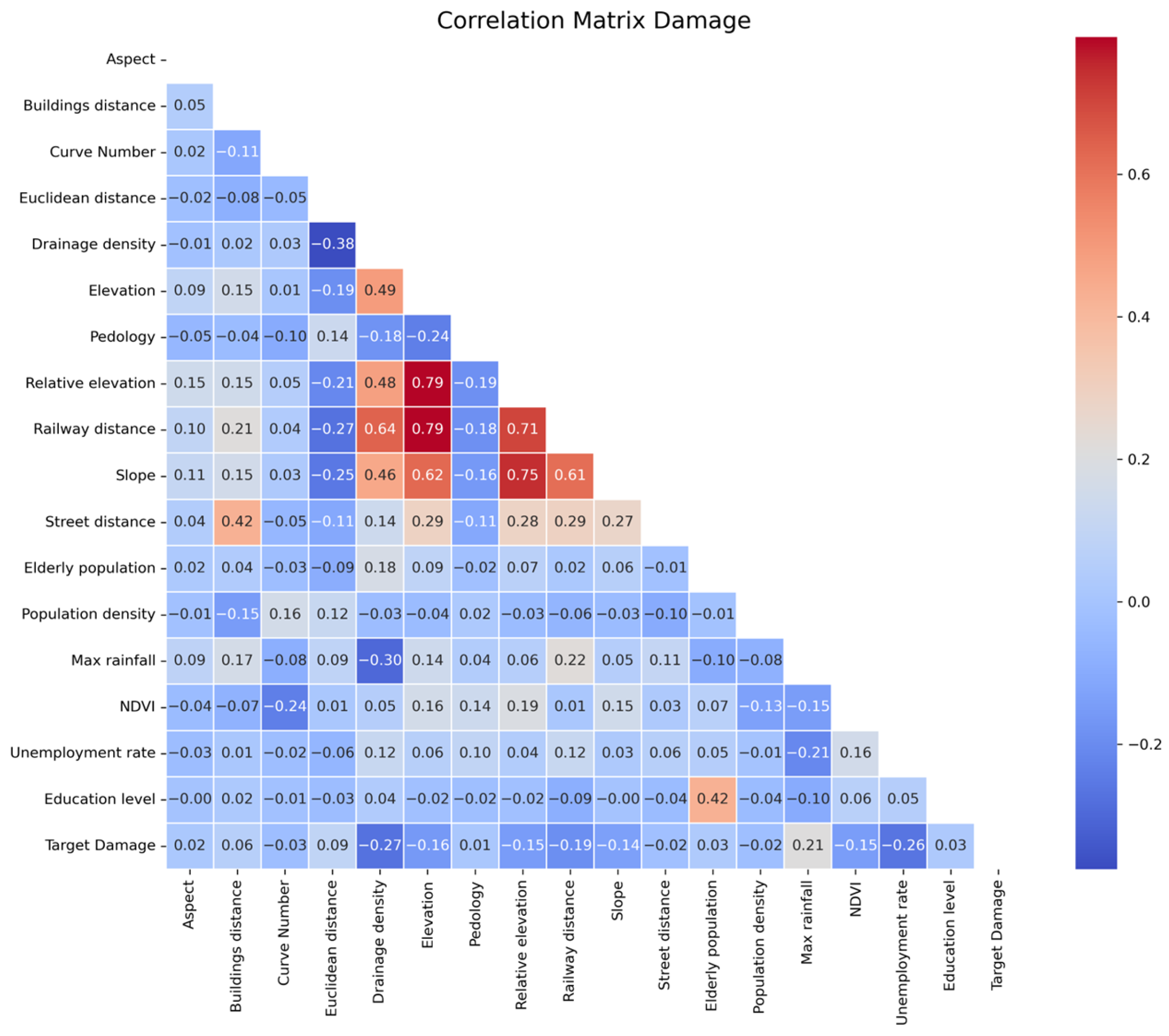
As a preliminary step of the analysis (step 2 in Section 2.4), the relationships among predictors and between each predictor and the target variable were assessed using Pearson correlation analysis, with the aim of identifying potential linear dependencies among the predictors and between each predictor and the target variable. The statistical significance of the correlations was evaluated using the corresponding p-values (Figure 5). The analysis involved predictors related to hazard (Aspect, Curve number, Drainage density, Elevation, Relative elevation, Slope, Pedology, Euclidean distance, NDVI, and Maximum rainfall), exposure (Distance to Buildings, Distance to Streets, Distance to Railways, and Population density), and vulnerability (Percentage of elderly population, Unemployment rate, and Education level).
Figure 5. Correlation matrix for the observed damage target.
The analysis highlighted the absence of strong linear relationships between the predictors and the observed damage variable. However, some moderate to relatively high correlations emerged among variables describing related physical or environmental processes. For instance, significant positive correlations were observed between Elevation and Relative elevation, Elevation and Slope, Relative elevation and Slope, as well as between Drainage density and some of these variables. In particular, the correlations between Elevation and Relative elevation, and between Railway distance and Elevation, reached a maximum value of approximately r = 0.79. Moreover, the positive correlation between Education level and Percentage of elderly population was confirmed. On the contrary, negative correlations were found between Drainage density and damage, and moderately negative correlations with Unemployment rate (Figure 5). The other linear relationships among predictors remained largely consistent with those observed for the satellite-based map.
Despite the presence of some moderate correlations, none were sufficiently strong to justify the exclusion of predictors from the model. Consequently, all variables were retained in the subsequent modelling phases, allowing the classification model to capture complex and non-linear interactions that cannot be fully described through a simple bivariate analysis.

3.2. Classification Model Performance

The performance of the XGBoost classification model was evaluated on the held-out test set using classification reports (Table 3), which provide a comprehensive and quantitative assessment of the model’s ability to distinguish between damaged (class 1) and non-damaged (class 0) areas. These reports include key binary classification metrics: Precision (proportion of predicted positives that are true positives), Recall (proportion of actual positives correctly identified), F1-score (harmonic mean of Precision and Recall), and overall Accuracy.
Table 3. Summary classification report for the satellite-observed target.
The model achieved excellent performance, with overall accuracy = 0.988, ROC-AUC (test set) = 0.996, F1-score for the minority class = 0.860, and macro-averaged F1 = 0.927. Precision, Recall, and F1-score were high for both classes (precision: 0.996 for class 0, 0.822 for class 1; recall: 0.992 for class 0, 0.903 for class 1), indicating robust discrimination, minimal false positives, and effective detection of actual damage instances. Weighted averages for Precision, Recall, and F1 were 0.989, 0.988, and 0.988, respectively, further confirming the balanced predictive performance across classes. These results are in line with state-of-the-art applications of ensemble tree-based models (e.g., XGBoost, Random Forest) in flood damage and susceptibility mapping, where accuracies frequently exceed 95–99% when geospatial predictors are combined with balanced training and rigorous hyperparameter tuning [30,59]. The high performance validates the model’s suitability for generating reliable probabilistic damage probability maps, particularly when trained on observed damage records that reflect actual flood impacts.
To complement the evaluation of predictive performance and account for spatial autocorrelation, a spatial block cross-validation was performed. Each block was used in turn as the test set, while SMOTE was applied exclusively within the training subset of each fold. The mean ROC-AUC across blocks was ≈0.674 (standard deviation = 0.18, range = 0.33–0.98) demonstrating the model’s robust generalization across spatially heterogeneous areas. These results confirm both the reliability of predictions on the held-out test set and the model’s ability to discriminate between damaged and non-damaged pixels in a spatially coherent manner.

3.3. Spatial Distribution of Damage Probability

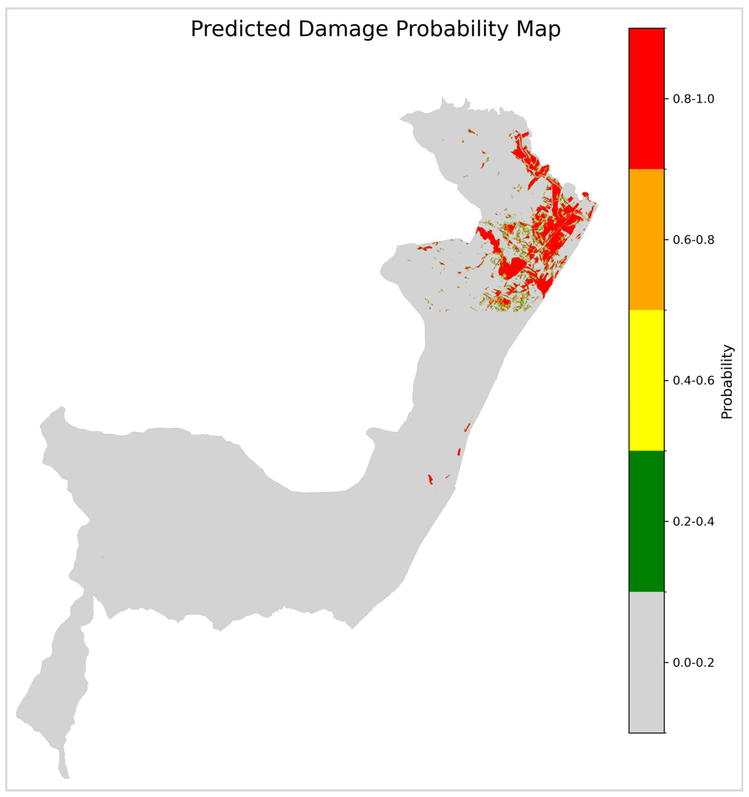
After verifying the good performance of the model, the probability of damage associated with each pixel of the study area was subsequently calculated. This probability represents a quantitative measure of the propensity to damage as a function of the combination of the predictors considered. In this way, the model does not merely provide a simple binary classification (damaged/non-damaged) but allows the expression of the degree of uncertainty associated with the prediction, offering a more informative and gradual assessment of the analyzed phenomenon. The probability estimated by the model assumes continuous values ranging from 0 to 1 and was used to construct a damage probability map, which was subsequently interpreted as a risk map. This interpretation is justified by the fact that the damage probability implicitly integrates the components of hazard, exposure, and vulnerability, allowing the combined effect of these factors on the spatial distribution of potential damage to be captured. This approach makes it possible to overcome a purely deterministic view of damage, providing a representation that is more consistent with the complexity of real territorial systems.
For improved cartographic interpretation, the continuous probability values were divided into five classes, each associated with a specific range of values and a representative color (Figure 6). In particular, areas characterized by null or very low damage probability (values close to 0.0) are represented in grey. Probability classes ranging from 0.2 to 0.4 are displayed in green, while intermediate values between 0.4 and 0.6 are shown in yellow. Areas with higher damage probability, ranging from 0.6 to 0.8, are highlighted in orange, whereas zones characterized by the highest probability of damage (0.8–1.0) are represented in red, indicating the areas at highest risk.
Figure 6. Spatial distribution of damage probability for the satellite-observed target.
The analysis of the probability map highlights that areas where the classifier correctly identified the presence of damage exhibit high probability values, predominantly associated with the highest classes (orange and red). These high-probability areas spatially correspond to the zones where damage was predominantly observed in the original target maps, confirming the spatial consistency of the model outputs. Conversely, areas classified as non-damaged are dominated by the grey color, indicating null or very low damage probability. Intermediate classes (green, yellow, and orange) are limited to small and localized spatial portions, suggesting transition areas or zones characterized by mixed territorial conditions, for which the model expresses a higher degree of uncertainty.
Overall, the spatial distribution of damage probability is consistent with the classification results and confirms the model’s ability to identify not only areas most exposed to damage, but also intermediate risk gradients. The resulting risk map therefore constitutes a decision-support tool, useful for identifying priority areas for intervention, for territorial planning, and for the definition of mitigation and adaptation strategies.

3.4. Feature Importance Analysis Based on SHAP Method

In order to ensure model transparency and to understand the role of individual predictors in risk estimation, an analysis based on Explainable Artificial Intelligence (XAI) techniques was conducted [55,60]. These methods are particularly relevant in the case of complex Machine Learning models, often considered “black-box” systems, as they allow the decision-making process to be interpreted and enable the analysis of how and why specific variables influence predictions.
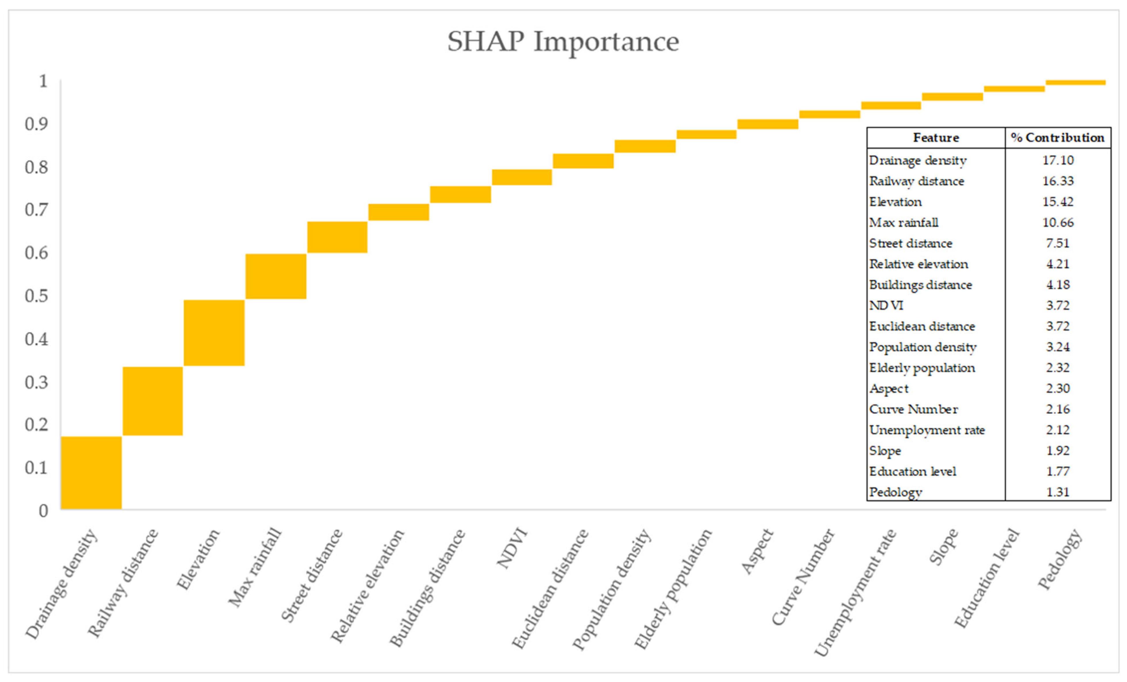
In this study, the SHapley Additive exPlanations (SHAP) method was adopted, which is grounded in cooperative game theory. SHAP assigns to each feature a weight proportional to its relevance within the model, ensuring properties of consistency and additivity [53,54]. Specifically, the SHAP value measures how much each predictor contributes to increasing or decreasing the probability of damage with respect to the average prediction value. Based on this approach, to evaluate the relative importance of the predictors within the model, the SHAP method was used. In particular, SHAP Feature Importance was computed in order to identify the variables that contribute the most to the estimation of damage probability. This measure is based on the mean absolute value of the SHAP contributions associated with each feature and allows the overall influence of the variables on the model predictions to be quantified, providing an interpretable evaluation of their role in the decision-making process [61]. The SHAP values were converted into relative percentages. For each feature, the mean absolute SHAP value across all samples was computed, and its percentage contribution was obtained by dividing this value by the sum of mean absolute SHAP values of all features and multiplying by 100. The results of this analysis are reported in Figure 7, which includes both the SHAP Feature Importance plot and the table of percentage contributions for each feature, making the relative weight of each predictor immediately clear.
Figure 7. SHAP Feature Importance of damage probability.
The analysis shows that the variables exerting the greatest influence on the model predictions are Drainage density (17.10%), Railway distance (16.33%), Elevation (15.42%), Max rainfall (10.66%), Street distance (7.51%), and Relative elevation (4.21%). This result highlights the combined role of the morphological characteristics of the territory and the proximity to infrastructures in the estimation of damage probability, suggesting that these factors represent key elements in defining flood-risk susceptibility within the study area.

3.5. SHAP Bee Swarm Plot for Global Interpretability

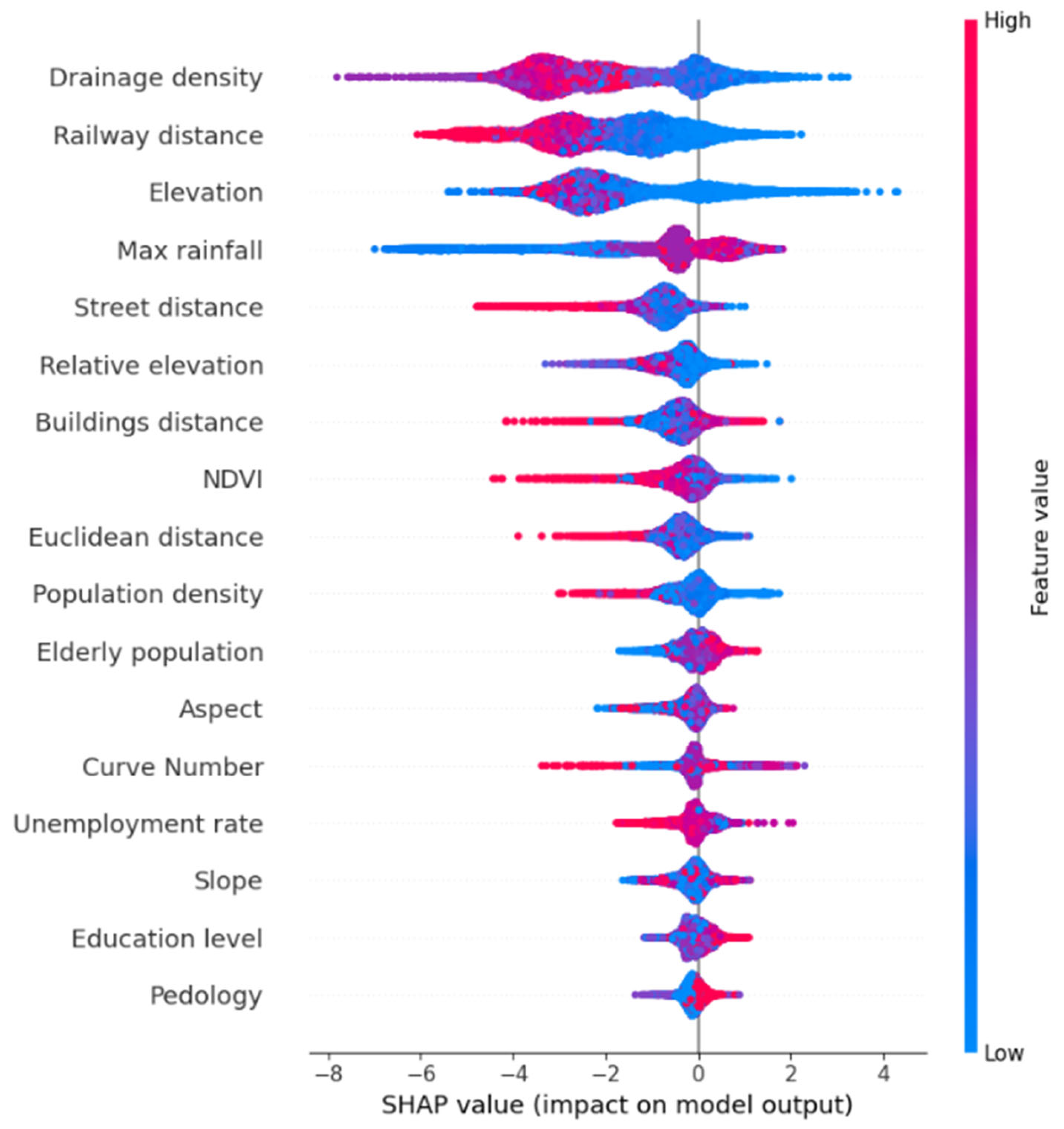
A global interpretability analysis of the model results was conducted using the Bee Swarm Plot representation of SHAP values (Figure 8) [56]. This graphical approach allows the distribution of SHAP values associated with each predictor to be examined, highlighting both the direction and magnitude of their contribution to the model output. In the plot, each point represents an individual observation, along the horizontal axis according to its SHAP value, while the color scale reflects the magnitude of the corresponding feature value.
Figure 8. SHAP Bee Swarm Plot of damage probability.
From the observation of the Bee Swarm Plot (Figure 8), the highest positive SHAP values are predominantly associated with low values of Drainage Density, Railway Distance, Elevation, Street Distance, and Relative Elevation, while they are associated with high values of Max Rainfall and Buildings distance. This indicates that conditions such as lower elevations, closer proximity to infrastructures, specific morphometric configurations, and higher rainfall tend to increase the model-estimated probability of damage. Moreover, high rainfall values are consistently associated with positive SHAP contributions, highlighting the role of intense precipitation in increasing the probability of damage. Regarding the distance from buildings, the model shows a positive contribution for higher values, suggesting a relationship that reflects the specific spatial characteristics of the study area.
Overall, the SHAP analysis highlights a consistent pattern, showing that topographic characteristics, rainfall conditions, and proximity to infrastructures are key determinants of damage probability. The combined interpretation of SHAP Feature Importance and Bee Swarm Plot provides an interpretable overview of the model’s global behavior and the contribution of the main predictors.

3.6. Comparative Assessment with Hydraulically Modeled Scenarios

In order to evaluate the consistency of the results obtained and to assess the behaviour of the model with respect to different representations of the phenomenon, a comparison was carried out between the modelling using the target related to the integrated dataset of recorded damages and satellite-observed flood areas, considered as the main reference of the study, and the three targets derived from hydraulic perimetric delineations (P1, P2, and P3), corresponding to different hazard scenarios. In particular, the analysis focused on the main variables identified as most influential in the models, examining the performance obtained, the Bee Swarm Plot, and the average trend of SHAP values.
Overall, the performance obtained (Table 4) is high for all the targets considered, with accuracy values and classification metrics being comparable among them.
Table 4. Summary classification report for the four targets.
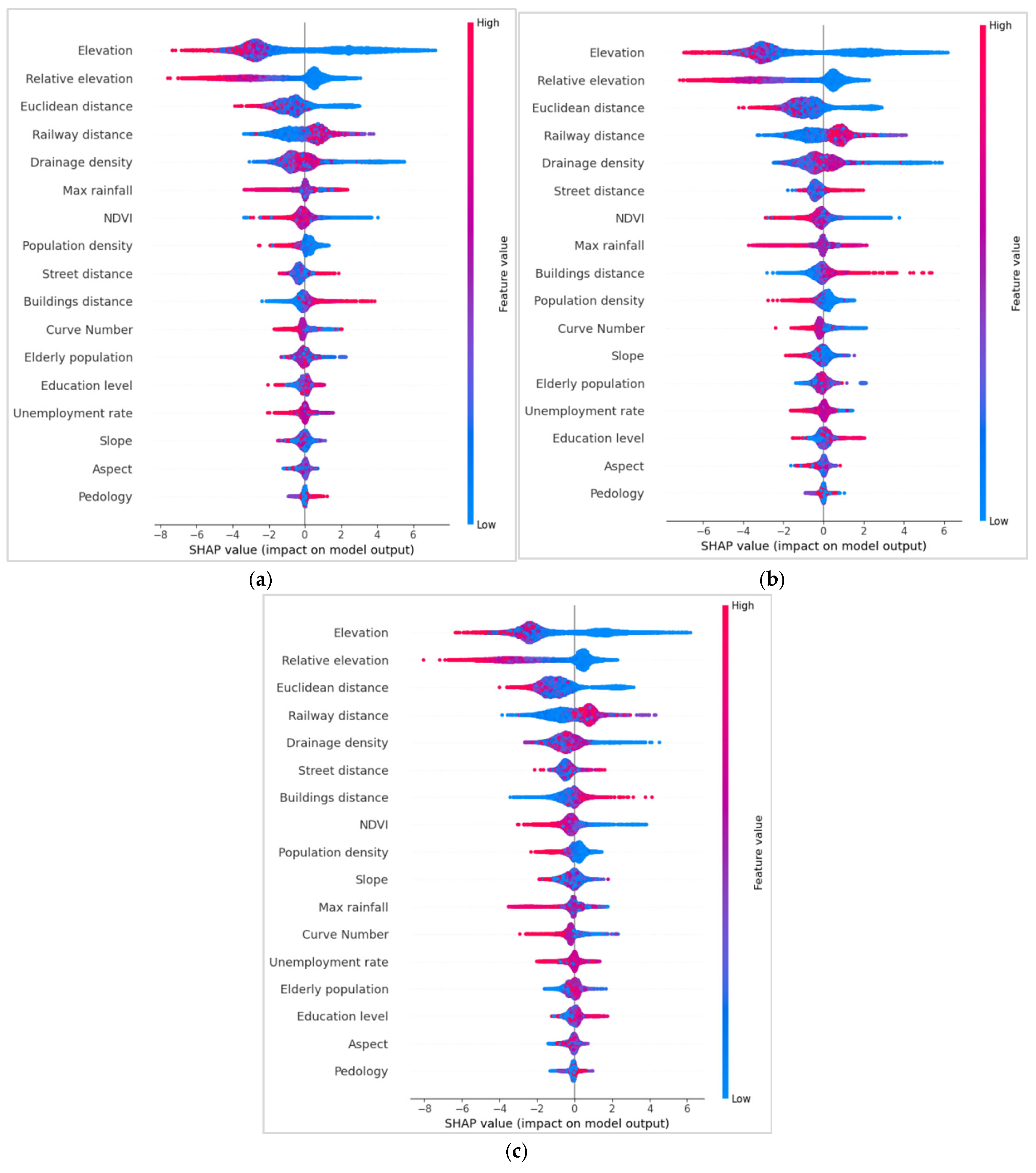
However, the comparative analysis of the interpretations provided by the SHAP method highlights some differences in the behavior of the variables. In the comparison of the Bee Swarm Plots (Figure 9a–c) of the different models (where Figure 9a corresponds to target P1, Figure 9b to target P2, and Figure 9c to target P3—a strong consistency emerges first and foremost among the results obtained for targets P1, P2, and P3.
Figure 9. SHAP Bee Swarm plots for the main predictors under the hydraulic scenarios: (a) P1 (500-year), (b) P2 (200-year), and (c) P3 (30-year).
In all three cases, in fact, the variables that are most relevant are substantially the same: Elevation, Relative elevation, Euclidean distance, Drainage density, Railway distance, and Street distance, although with slight variations in the order of importance. A particularly evident element in the Bee Swarm Plots of the three models concerns the relationship between the value of the variables and the intensity of their contribution to the model. For almost all the features considered, the highest SHAP values are associated with low values of the variables, indicating that conditions of greater susceptibility are generally related to low elevations, reduced distances from infrastructure, and specific morphometric configurations. This behavior appears consistent among the three targets derived from the perimetric delineations. An exception is represented by the variable Railway distance, for which the Bee Swarm Plot shows a less clear distribution: in the area of the plot associated with the highest SHAP values, both points associated with high values and points associated with low values are present, making the identification of a monotonic relationship between distance from the railway and model contribution less immediate.
The comparison with the Bee Swarm Plot related to the integrated dataset of recorded damages and satellite-observed flood areas shows some interesting differences (Figure 8). In this case as well, apart from the order of importance, the most influential variables are largely coincident with those identified in the P1, P2, and P3 target models; however, in the case of the integrated dataset, it becomes more evident that the highest contributions of the model are uniquely associated with low values of all the main variables, confirming the role of low-lying areas close to infrastructures as the conditions most predisposing to damage. Moreover, in the case of the observed dataset, the role of the Max rainfall variable emerges more clearly, taking on a relatively greater importance compared to the other scenarios. This result is consistent with the nature of the phenomenon under investigation, as the damages considered are directly related to flood events triggered by intense precipitation.
Overall, therefore, the analysis of the Bee Swarm Plots highlights on one hand a good consistency among the models built on the three perimetric scenarios and, on the other hand, some differences compared to the model trained on the integrated dataset, suggesting that different definitions of the target may influence, at least in part, the relative weight assigned to the explanatory variables.
To strengthen the comparison and address the reviewer’s request for quantitative assessment, a quantitative spatial evaluation was performed between the susceptibility maps derived from the integrated dataset and those obtained from the hydraulic scenarios (P1, P2, and P3). Specifically, the comparison was carried out by computing the F1-score, the Intersection over Union (IoU), and the Pearson correlation coefficient between the observed damage map and the predicted susceptibility maps. The binary maps used for F1 and IoU computation were obtained by applying an optimal threshold identified through Youden’s J statistic.
The results show moderate levels of spatial agreement, with F1 values ranging from 0.32 to 0.38 and IoU values between 0.19 and 0.23. The Pearson correlation coefficients range from 0.32 to 0.40, indicating a non-negligible correspondence between the spatial patterns of observed damages and model predictions. Among the considered scenarios, P3 consistently exhibits the highest agreement with the observed data across all metrics, suggesting that this configuration provides a more representative approximation of the actual damage distribution. Overall, these results indicate that, although the hydraulic scenarios are not able to fully reproduce the spatial distribution of observed damages, they capture relevant patterns of susceptibility. This partial agreement is consistent with the complexity of flood-related damage processes, which are influenced not only by hydraulic conditions, but also by additional environmental and infrastructural factors.

3.7. Identification of Critical Risk Thresholds Using Partial Dependence Plot (PDP)

To translate the relationships observed in the global interpretability analysis into actionable insights, the effect of the most influential variables on model predictions was examined using Partial Dependence Plots (PDP).
Building on the global interpretability results, six variables consistently identified as the most influential across all four models (observed damage, P1, P2, and P3) were selected for detailed analysis: Drainage density, Railway distance, Elevation, Max rainfall, Street distance, and Relative elevation.
For each variable, PDP curves were produced to show the relationship between feature values and the predicted probability of damage. These plots provide a clear and interpretable visualization of how each predictor influences the model output.
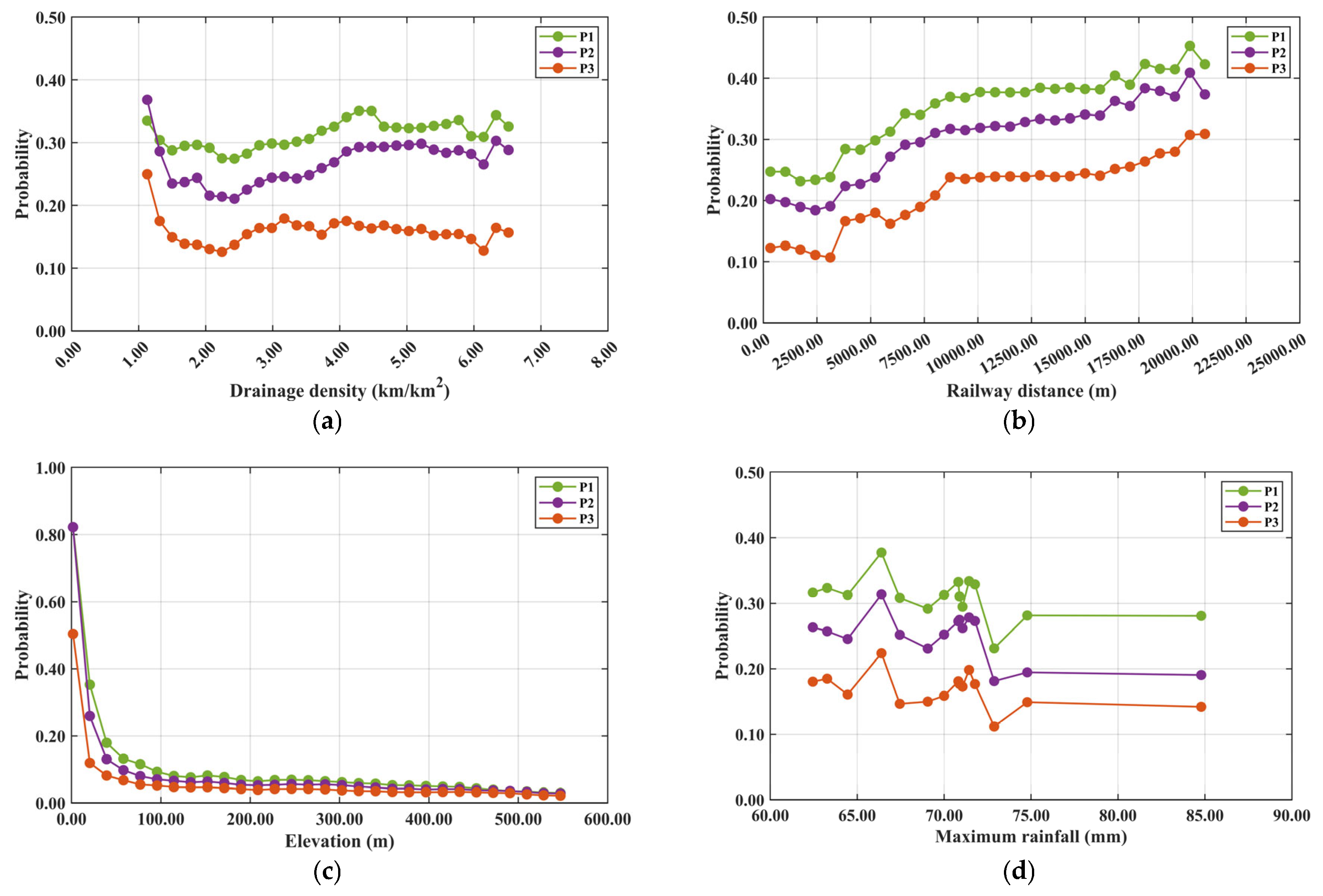
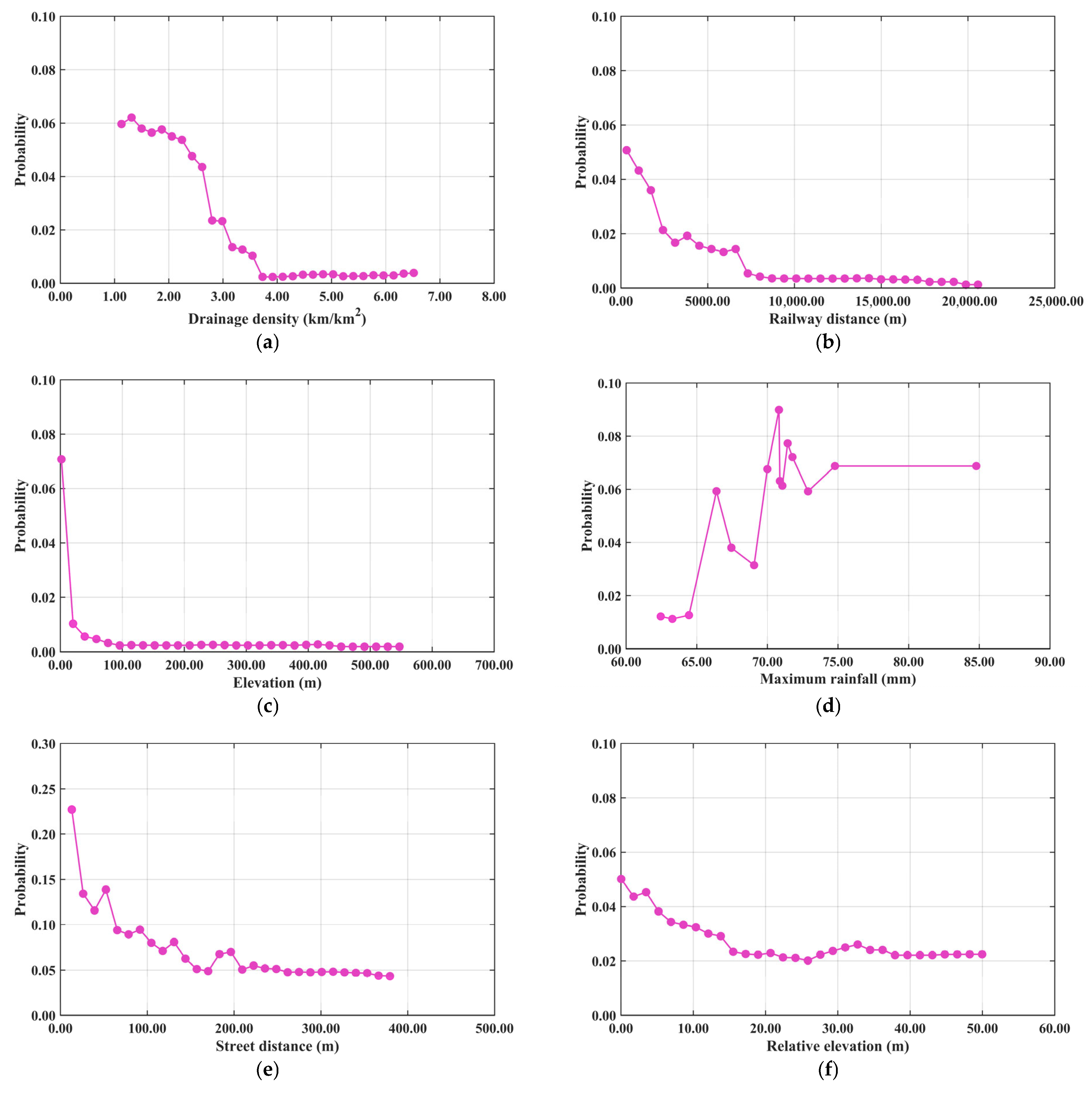
The analysis focused on the trends of the PDP curves to identify critical thresholds for each feature. For the main target, six plots were produced (Figure 10a–f), one for each selected feature, showing the corresponding PDP curves for the integrated target. The identified thresholds indicate the conditions under which each variable has a significant effect on the predicted probability of damage. The PDPs indicate that the model is mainly driven by nonlinear, threshold-based relationships: some variables exhibit a pronounced decreasing effect, while others influence the output only after specific ranges are exceeded. Overall, the plots suggest that the model response depends on a limited number of critical intervals rather than on uniform changes across the entire domain.
Figure 10. Partial Dependence Plot (PDP) of the most important features of the satellite-observed damage target (panels (af)).
The model appears to be particularly sensitive to proximity to infrastructure as well as to topographic and rainfall conditions within well-defined thresholds. The variables showing the strongest effects are street distance, railway distance, drainage density, and elevation, all of which are characterized by a rapid decrease followed by saturation. In contrast, max rainfall is the only variable displaying a clearly increasing and threshold-dependent behaviour. This overall pattern of PDPs is consistent with a model that captures strong nonlinearities, operational thresholds, and potential interactions among environmental predictors.
In summary, the PDPs highlight a predominantly nonlinear and threshold-driven response: distance from roads and railways, drainage density, and elevation show decreasing effects with saturation, whereas max rainfall increases the predicted output beyond a critical threshold, suggesting that spatial configuration and extreme rainfall conditions play a key role within specific ranges.
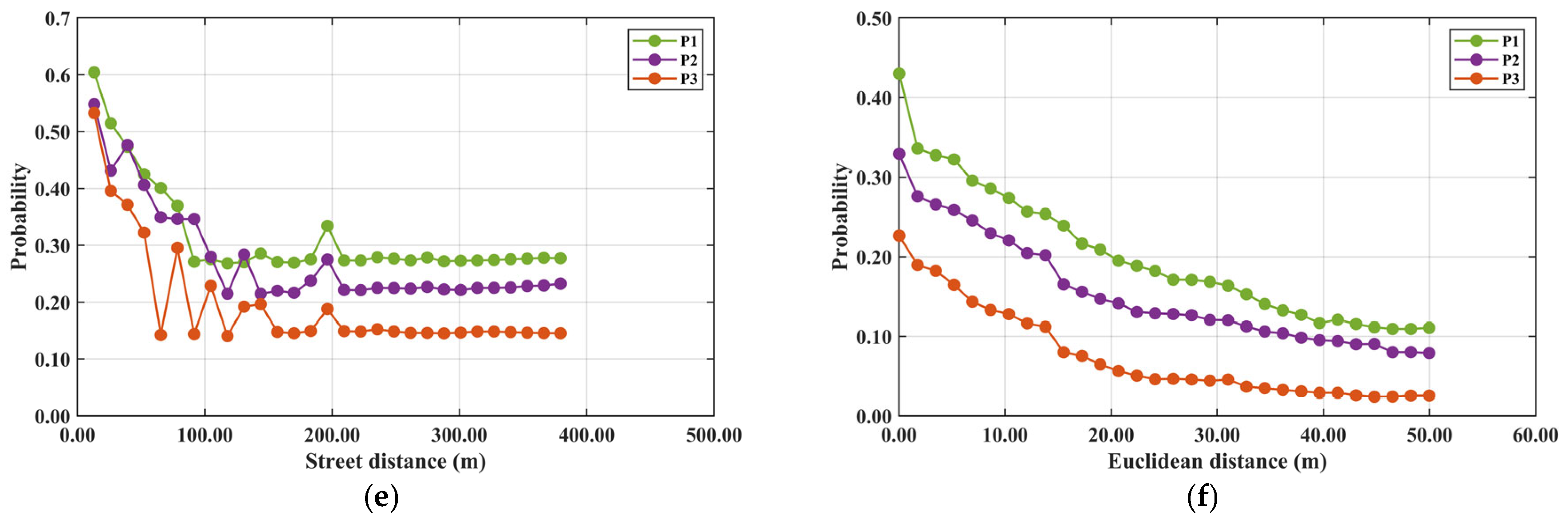
For the three targets derived from the P1, P2, and P3 models, six comparative graphs were produced (one for each selected feature), in which the PDP curves for the three targets are displayed in the same graph using different colors for each model. This visualization allows a direct comparison of the effect of each feature on the predicted probability of damage across the different scenarios (Figure 11a–f).
Figure 11. Partial Dependence Plot of the most important features of the P1, P2 and P3 targets (panels (af)).
The procedure was applied to all six main variables for each of the three modeled targets, providing a consistent and interpretable basis for assessing how critical thresholds vary depending on the hydraulic scenario. This approach enables the identification of feature ranges where the predicted probability of damage significantly changes, offering an objective and quantitative framework for comparing risk patterns across models.
The model using the P1 target shows higher response values and, in some cases, more gradual relationships. Overall, threshold and saturation effects are still evident, but with a less extreme and more smoothed structure. Overall, these PDPs describe a model that combines decreasing, increasing, and saturating effects, although with different intensities across variables. Elevation, relative elevation, and street distance appear to play a more structured and interpretable role, whereas drainage density and max rainfall show weaker or locally non-monotonic relationships. Railway distance, on the other hand, is the predictor exhibiting an opposite relationship compared to urban proximity variables. In summary, the PDPs show that the model is dominated by nonlinear threshold and saturation relationships: elevation, relative elevation, and street distance exert a decreasing effect, railway distance shows an increasing effect, while drainage density and max rainfall exhibit weaker or locally non-monotonic patterns.
The PDPs related to the P2 target show stable and interpretable relationships: some variables exhibit a clear decreasing effect, others show an increasing effect, while drainage density and max rainfall display weaker or slightly non-monotonic patterns. The model therefore appears to respond mainly to threshold and saturation effects rather than to constant linear variations.
The model seems to be driven primarily by topographic and spatial proximity relationships: elevation, relative elevation, street distance, and railway distance show the most clearly defined patterns. Among these, elevation and relative elevation act in a negative direction, whereas railway distance is the only variable with a clearly positive trend. Drainage density and max rainfall are instead weaker or less monotonic, suggesting a secondary role or an influence conditioned by interactions. In summary, the PDPs indicate that the model is dominated by nonlinear saturation-based relationships: elevation and relative elevation show a decreasing effect, railway distance shows an increasing effect, street distance shows a strong initial decrease followed by a plateau, while drainage density and max rainfall exhibit weaker or locally non-monotonic patterns.
Finally, with reference to the P3 target, the PDPs show a fairly consistent pattern: the model is mainly driven by nonlinear, threshold-based relationships with saturation effects. Topographic and distance-related variables exhibit the clearest patterns, whereas drainage density and max rainfall appear weaker or less monotonic.
Overall, elevation, relative elevation, and street distance are the variables with the clearest negative effects, while railway distance shows the most evident positive effect. Drainage density and max rainfall instead display less linear patterns and are likely more dependent on interactions. This configuration suggests that the model primarily exploits spatial and topographic gradients, with some well-defined operational thresholds.
In summary, the PDPs (Figure 11a–f) indicate that the model is dominated by nonlinear threshold and saturation relationships: elevation, relative elevation, and street distance show a decreasing effect, railway distance shows an increasing effect, while drainage density and max rainfall exhibit weaker or locally non-monotonic patterns.
Building on the previous results, the following analysis provides a detailed interpretation of the Partial Dependence Plots (PDPs), illustrating how each predictor influences the model output across the observed target and the simulated scenarios (P1–P3).
Considering the feature Drainage density (unitless index), the observed target (OBS) shows a clearly negative and threshold-driven relationship. For low values (approximately 1.1/2.5 km/km2), the model predicts relatively high outputs, while a sharp decline occurs between about 2.7 km/km2 and 3.6 km/km2, leading to an almost complete flattening beyond 3.8 km/km2. This indicates that the model is mainly sensitive to the transition from low to intermediate drainage density values, while higher values correspond to a saturation effect where the marginal contribution becomes negligible. In P1, the relationship becomes much flatter and less structured. The curve shows only mild oscillations within a narrow range (approximately 0.27–0.35). This indicates that the variable has a weak but non-zero effect: the model uses it, but without a strong monotonic direction. It can be interpreted as a slightly non-linear relationship, with a small minimum around 2/2.5 km/km2 and a maximum around 4/4.5 km/km2. In P2, the pattern remains generally flat but slightly more structured than in P1. A shallow minimum emerges around 2.0/2.6 km/km2, followed by a gradual increase towards higher values (approximately 4.5/5.5 km/km2). This suggests a weak and non-monotonic relationship, where the variable contributes mainly in interaction with other features rather than acting as a dominant driver. Finally, in P3 the curve shows a mild non-monotonic behaviour: values start relatively high, decrease between approximately 1.5 km/km2 and 2.5 km/km2, and then slightly recover before stabilising at intermediate levels. Overall, the effect remains secondary, with no clear monotonic trend, indicating that the model uses Drainage density mainly for local adjustments rather than as a primary explanatory factor.
Passing to the feature Elevation, the observed target (OBS) shows a very strong effect at low values, with a rapid initial decrease followed by an almost complete flattening at very low prediction levels. The model is particularly sensitive to low elevations, with a main PDP threshold emerging around 25/35 m, beyond which additional increases in elevation provide little information. This behaviour is consistent with an inverse and saturating relationship. In P1, elevation shows a clearly decreasing pattern: at very low values predictions are high, then they drop rapidly and continue decreasing more gradually until stabilising at lower levels. This is a typical inverse profile with strong initial sensitivity and later saturation, with the main threshold shifting to approximately 40/60 m. Low elevations therefore have a much stronger impact than intermediate and high values. In P2, elevation exhibits a strongly decreasing relationship: low values correspond to high outputs, but predictions drop rapidly in the initial intervals and then continue decreasing more slowly. This is a classic saturation pattern, where the early part of the range carries most of the explanatory power, with a main threshold located around 50/70 m. The model therefore associates low elevations with more favourable conditions for the predicted outcome. Finally, in P3, elevation shows a clearly decreasing relationship: low altitude values correspond to high predictions, but the curve drops rapidly within the first intervals and then flattens. This inverse saturating effect is maintained, with the main threshold further shifting to approximately 60/90 m. The model continues to assign much greater importance to low elevations compared to medium and high ones, although the sensitivity range expands across scenarios.
Moving to the feature Max rainfall, the observed target (OBS) shows a very clear positive and threshold-driven behaviour. For values below approximately 63/65 mm, predictions remain low, while a sharp increase occurs between about 66 mm and 72 mm, with a peak around 70/71 mm. This suggests a step-like response, where rainfall becomes relevant only beyond a certain intensity level. The dispersion observed in the upper range indicates that, although this variable is important, it likely interacts with other predictors in determining the final output. In P1, max rainfall is concentrated within a relatively narrow interval (approximately 63/73 mm), with a peak around 66/68 mm and some lower values closer to 74/76 mm. The relationship is not strictly monotonic: instead, there appears to be an optimal range where predictions are maximised, while beyond this interval the effect slightly decreases. This behaviour suggests potential interactions with other variables or a model sensitivity to intermediate–high rainfall extremes. In P2, max rainfall remains confined to a narrow range (approximately 63/76 mm), with a peak around 66/70 mm and a slight reduction beyond this interval. No clear monotonic relationship emerges; instead, the variable shows a threshold-like behaviour with a preferred range of maximum impact. This is consistent with a response influenced by interactions with other climatic or topographic predictors. Finally, in P3, max rainfall continues to exhibit a similar pattern, with values concentrated between approximately 63 mm and 76 mm and the highest responses around 66/71 mm. The relationship remains non-monotonic, but a clear band of maximum sensitivity emerges at high but not extreme precipitation levels. This confirms a threshold-based behaviour, likely driven by interactions between rainfall intensity and other explanatory variables.
Considering the feature Railway distance, the observed target (OBS) shows a very strong decreasing and threshold-driven relationship. Very low distances from the railway correspond to high predictions, but the effect drops rapidly and then stabilises at an almost negligible level beyond approximately 7000/8000 m. This indicates a clear attenuation effect, where proximity to the railway is relevant only within a limited spatial range, while beyond a certain threshold the model becomes largely insensitive to further increases in distance. In P1, railway distance shows a clear positive relationship: as distance increases, predictions rise from lower values up to a higher plateau. The increase is more pronounced in the initial segments and then gradually attenuates, becoming almost stable beyond approximately 10,000/12,000 m. This suggests that, in this scenario, greater distance from the railway is associated with higher output values. In P2, railway distance exhibits a strongly positive and more continuous trend: predictions increase from approximately 0.18–0.20 to values above 0.40 as distance grows. The rise is steeper in the first 5000/8000 m, after which the curve tends to stabilise with only a slight additional increase. This confirms that the model associates greater railway distance with higher predicted outcomes. Finally, in P3, railway distance maintains a generally increasing and smooth relationship: as distance increases, model responses grow and then stabilise at higher levels. The most significant change occurs within the first 8000/10,000 m, while beyond this range the curve increases more slowly. This confirms a consistent positive association between railway distance and the predicted output across the scenario.
Analysing the feature Relative elevation, the observed target (OBS) shows an initial decreasing behaviour followed by a quasi-flat region with a slight intermediate rebound and a subsequent stabilisation. The model is more sensitive to low values, while in the mid-to-high range the effect becomes weak and almost constant. A main threshold is observed around 12/18 m, indicating that most of the explanatory power is concentrated at low relative elevation values, while higher values contribute marginally to the prediction. In P1, relative elevation exhibits a clear and almost linear decreasing pattern, with predictions dropping from higher initial values to a lower plateau. The relationship is strongly negative, indicating that lower relative elevation is associated with higher model responses. The effect is more pronounced at the beginning and progressively weakens towards the end, with a main threshold around 15/25 m, reflecting a gradual saturation of the effect. In P2, relative elevation maintains a similar structure, with a regular and almost linear decrease from high initial values to a low plateau. The relationship is particularly clear in this scenario, with lower relative elevation corresponding to lower predicted values. The decline is steep in the early range and then slows down, with a main threshold around 10/20 m, again indicating progressive saturation of the effect. Finally, in P3, relative elevation shows a smooth and well-structured decreasing pattern: high initial values progressively decline until reaching a low plateau. The relationship is strongly negative and close to monotonic, making it one of the most stable patterns across features. The main threshold is observed around 12/22 m, confirming that the strongest sensitivity remains concentrated in the low relative elevation range, while the effect stabilises in the higher range.
Finally, considering the feature Street distance, the observed target (OBS) shows a strong negative relationship at low values, with very high predictions for small distances and a progressive decrease as distance increases. After approximately 150/200 m, the curve flattens, indicating a clear saturation effect: beyond this threshold, further increases in distance have a negligible impact on the model output. This reflects a strong spatial gradient that becomes stable once a certain distance is exceeded. In P1, street distance shows a very steep decline in the initial range, followed by an almost complete stabilisation at an intermediate level. This indicates that proximity to streets has a strong influence only up to a certain distance, while beyond that point the effect becomes nearly constant. A small local increase around 190/200 m is observed, likely due to sampling sparsity or interaction effects. In P2, street distance exhibits a sharp initial decrease followed by a stable plateau around 0.22–0.23. The variable has a strong effect only at short distances, while beyond approximately 120/150 m the response becomes flat. A small, isolated increase around 190/200 m is visible but is likely attributable to local variability or sampling artefacts. The main threshold is therefore located around 120/150 m, after which the model output remains largely unchanged. Finally, in P3, street distance shows a pronounced drop at low values followed by a long and stable plateau. The model response decreases rapidly within the first distance intervals and then stabilises, indicating that most of the explanatory power is concentrated below approximately 120/150 m. Beyond this threshold, additional distance contributes minimally to the prediction, confirming a strong saturation effect in the spatial relationship.

4. Discussion

The results from the XGBoost model applied to the observed damage target high-light the critical role of physical and hydrological factors in driving flood damage susceptibility along the Basilicata Ionian coast, with Drainage density emerging as the dominant predictor (17.10% importance). This finding aligns with the region’s geomorphological characteristics, where dense channel networks in erodible clay-sandy formations facilitate rapid runoff and overflow during short, intense rainfall events, as observed in historical floods like those in autumn 2013 (which caused about 45 million euros of damages in the Metaponto plain) and recurrent episodes in the last two decades [32,36,37]. Elevation (15.42%) and Relative elevation (4.21%) further underscore topographic vulnerabilities, with low-lying areas (E ≤ 25/35 m) prone to water accumulation in coastal plains such as the Metaponto, consistent with Bentivenga et al. (2020) [62] on morphodynamic activity in Lucanian basins. The PDP thresholds provide enhanced interpretability by identifying operational risk thresholds for the observed target: Drainage density (transition around 2.7/3.6 km/km2, with saturation beyond 3.8 km/km2; unitless index), Elevation ≤ 25/35 m, Max rainfall approximately 63/72 mm, Railway distance ≤ 7000/8000 m, Relative elevation ≤ 12/18 m, and Street distance ≤ 150/200 m—where risk amplifies non-linearly, extending traditional hydrodynamic models (e.g., [63]) that often lack such granular, empirically grounded insights from real damage records.
Exposure factors, contributing ~37–40% overall (e.g., Street distance 7.51%, Railway distance 16.33%), reveal how proximity to infrastructure exacerbates damages in urbanized zones, amplifying economic losses in transport corridors near the Bradano and Basento rivers. This supports recent findings on infrastructure’s role in flash flood risks in southern Italy [7,10] and aligns with global patterns where dense man-made infrastructure intersects with hazards to increase vulnerability [8]. Max rainfall (10.66%) and NDVI (3.72%) thresholds capture climatic and environmental drivers, linking to climate change-induced storm intensification in Mediterranean contexts [6], though their moderate importance suggests event-specific variability. However, the importance of both maximum rainfall and NDVI may be constrained by the downscaling process, in which high-resolution data are resampled to a common analysis grid using the nearest-neighbor interpolation method.
Vulnerability factors showed limited influence (<4% combined), with elderly population (2.32%) and unemployment rate (2.12%) minimally impacting predictions. This may stem from the model’s training on institutional damage reports focused on physical/infrastructural failures rather than direct human casualties or socio-economic impacts, echoing gaps in Italian studies where social vulnerability is often assessed separately [32]. In addition, these variables exhibit relatively low spatial variability across the study area, as coastal municipalities along the Ionian coast of Basilicata are demographically homogeneous compared to the strong geomorphological and proximity gradients of the dominant predictors. Consequently, their reduced discriminative power is reflected in lower SHAP values, which likely indicate limited spatial variability rather than negligible causal relevance. The predominance of hazard and exposure aligns with the research hypothesis that integrating observed damage data prioritizes observable, threshold-like patterns, addressing limitations in conventional models that overlook real-world records [8,15].
Compared to the hydraulically modeled scenarios (P1–P3), the observed-damage map exhibits sharper, threshold-driven patterns (e.g., abrupt risk increases below low elevation or near infrastructure), while modeled extents produce smoother, continuous gradients that contract with increasing return period. This contrast underscores the added value of the data-driven approach: hydraulic simulations excel at probabilistic hazard delineation but under-represent non-linear damage translation in infrastructure-proximate zones, where empirical evidence shows amplified impacts. The framework thus complements traditional flood hazard mapping by explicitly modeling where inundation translates into actual damage, offering more targeted insights for Mediterranean coastal regions.
These findings have broad implications for flood management in similar Mediterranean settings, enabling data-driven prioritization of interventions such as channel maintenance and desilting in high-drainage density areas, elevation-based zoning restrictions in low-lying coastal plains, and enhanced protection of linear infrastructure (e.g., roads and railways) near river corridors. The PDP-derived thresholds provide quantitative, operational guidance for land-use regulation and civil protection planning, supporting the EU Floods Directive’s risk-based approach by bridging empirical observations with ML explainability.
Limitations include reliance on historical damage data (primarily 2006–2018), which may not fully capture emerging climate scenarios or future extremes, and the exclusion of dynamic factors like sea-level rise or compound events. Potential biases in institutional reporting, particularly the underrepresentation of minor damages, may affect the reliability of the damage dataset. Additional uncertainty may arise from the downscaling to a 20 m spatial resolution, especially for CHIRPS rainfall and MODIS NDVI data. Furthermore, the availability of reliable observed rainfall data during the flooding events was limited. Future studies should consider incorporating higher-resolution precipitation products where available.

5. Conclusions

This study demonstrates the value of an explainable XGBoost + SHAP framework for mapping flood damage susceptibility using observed institutional and remote-sensing damage records together with 17 geospatial predictors.
The model achieved excellent discrimination against damaged vs. non-damaged locations (accuracy ~98.8% on test set for the observed target) and revealed that damage occurrence is mainly controlled by drainage density (~17.1%), elevation (~15.4%), and proximity to transport infrastructure (~23.8% combined), with clear threshold-like patterns.
Compared to official hydraulic hazard zones (30-, 200- and 500-year return periods), the damage-based map captures sharper risk transitions and highlights infrastructure-proximate amplification zones that are less evident in modelled extents.
The methodology offers a replicable, data-driven complement to traditional flood hazard mapping and can support targeted mitigation actions in Mediterranean coastal floodplains—including desilting of dense channel networks, land-use restrictions in low-lying areas, and protection of critical linear infrastructure.
Future developments could focus on the integration of dynamic climate projections, compound-hazard assessment (flood + coastal processes), and enrichment of vulnerability indicators with direct socio-economic impact data.

Author Contributions

Conceptualization, S.F.D.S. and V.T.; methodology, S.F.D.S. and V.T.; software, M.R. and H.H.A.; validation, S.F.D.S. and V.T.; formal analysis, S.F.D.S. and V.T.; investigation, M.R., H.H.A., S.F.D.S. and V.T.; data curation, M.R., H.H.A., S.F.D.S. and V.T.; writing—original draft preparation, M.R., H.H.A., S.F.D.S. and V.T.; writing—review and editing, M.R., H.H.A., S.F.D.S. and V.T.; visualization, M.R., H.H.A., S.F.D.S. and V.T.; supervision, S.F.D.S. and V.T. All authors have read and agreed to the published version of the manuscript.

Funding

This research received no external funding.

Data Availability Statement

The datasets presented in this study are not publicly available because they were provided by institutional authorities and are subject to data-sharing restrictions. Requests to access the datasets should be directed to the competent local authorities, subject to their approval.

Acknowledgments

The authors would like to thank the Italian Department of Civil Protection of the Basilicata Region and the Southern Apennines District Basin Authority for providing the data and information used in this study.

Conflicts of Interest

The authors declare no conflicts of interest.

Appendix A

Figure A1. Hazard maps: (a) drainage density (b) elevation, (c) max rainfall, (d) Euclidean distance, (e) NDVI, (f) relative elevation, (g) curve number, (h) pedology, (i) aspect, and (j) slope.
Figure A2. Exposure maps: (a), street distance, (b) railway distance, (c) buildings distance, and (d) population density.
Figure A3. Vulnerability maps: (a) elderly population, (b) unemployment rate, and (c) education level.

References

  1. EC. Directive 2007/60/EC of the European Parliament and of the Council of 23 October 2007 on the assessment and management of flood risks. Off. J. Eur. Union 2007, 288, 27–34.
  2. Jongman, B.; Ward, P.J.; Aerts, J.C.J.H. Global exposure to river and coastal flooding: Long term trends and changes. Glob. Environ. Change 2012, 22, 823–835. [Google Scholar] [CrossRef] [Scilit]
  3. Lyu, H.M.; Shen, S.L.; Zhou, A.; Yang, J. Perspectives for flood risk assessment and management for mega-city metro system. Tunn. Undergr. Space Technol. 2019, 84, 31–44. [Google Scholar] [CrossRef] [Scilit]
  4. Hapuarachchi, H.A.P.; Wang, Q.J.; Pagano, T.C. A review of advances in flash flood forecasting. Hydrol. Process. 2011, 25, 2771–2784. [Google Scholar] [CrossRef] [Scilit]
  5. EEA. Economic Losses from Climate-Related Extremes in Europe. Available online: https://www.eea.europa.eu/ims/economic-losses-from-climate-related (accessed on 18 February 2026).
  6. Bhattarai, S.; Parajuli, P.B.; To, F. Comparison of flood frequency at different climatic scenarios in forested coastal watersheds. Climate 2023, 11, 41. [Google Scholar] [CrossRef] [Scilit]
  7. Rondinone, M.; Dal Sasso, S.F.; Aung, H.H.; Contillo, L.; Dimola, G.; Schiattarella, M.; Fiorentino, M.; Telesca, V. Assessing flood and landslide susceptibility using XGBoost: Case study of the Basento river in southern Italy. Appl. Sci. 2025, 15, 5290. [Google Scholar] [CrossRef] [Scilit]
  8. Dey, H.; Haque, M.M.; Shao, W.; VanDyke, M.; Hao, F. Simulating flood risk in Tampa Bay using a machine learning driven approach. npj Nat. Hazards 2024, 1, 40. [Google Scholar] [CrossRef] [Scilit]
  9. Romali, N.S.; Yusop, Z. Flood damage and risk assessment for urban area in Malaysia. Hydrol. Res. 2021, 52, 142–159. [Google Scholar] [CrossRef] [Scilit]
  10. Balestra, F.; Del Vecchio, M.; Pirone, D.; Pedone, M.A.; Spina, D.; Manfreda, S.; Menduni, G.; Bignami, D.F. Flood susceptibility mapping using a deep neural network model: The case study of southern Italy. Environ. Sci. Proc. 2022, 21, 36. [Google Scholar]
  11. Dawson, G.; Butt, J.; Jones, A.; Fraccaro, P. Flood susceptibility mapping at the country scale using machine learning approaches. Appl. AI Lett. 2023, 4, e88. [Google Scholar] [CrossRef] [Scilit]
  12. Albertini, C.; Gioia, A.; Iacobellis, V.; Petropoulos, G.P.; Manfreda, S. Assessing multi-source random forest classification and robustness of predictor variables in flooded areas mapping. Remote Sens. Appl. Soc. Environ. 2024, 35, 101239. [Google Scholar] [CrossRef] [Scilit]
  13. Hitouri, S.; Mohajane, M.; Lahsaini, M.; Ali, S.A.; Setargie, T.A.; Tripathi, G.; D’Antonio, P.; Singh, S.K.; Varasano, A. Flood susceptibility mapping using SAR data and machine learning algorithms in a small watershed in northwestern Morocco. Remote Sens. 2024, 16, 858. [Google Scholar] [CrossRef] [Scilit]
  14. Navarro, J.S.; Zhuang, R.; Albertini, C.; Manfreda, S. Mapping flood susceptibility using Random Forest exploiting satellite observations and geomorphic features. Sci. Total Environ. 2025, 1002, 180592. [Google Scholar] [CrossRef] [Scilit] [PubMed]
  15. Gain, A.K.; Mojtahed, V.; Biscaro, C.; Balbi, S.; Giupponi, C. An integrated approach of flood risk assessment in the eastern part of Dhaka City. Nat. Hazards 2015, 79, 1499–1530. [Google Scholar] [CrossRef] [Scilit]
  16. Gabriels, K.; Willems, P.; Van Orshoven, J. A comparative flood damage and risk impact assessment of land use changes. Nat. Hazards Earth Syst. Sci. 2022, 22, 395–410. [Google Scholar] [CrossRef] [Scilit]
  17. Meyer, V.; Haase, D.; Scheuer, S. Flood risk assessment in European river basins--concept, methods, and challenges exemplified at the Mulde River. Integr. Environ. Assess. Manag. 2009, 5, 17–26. [Google Scholar] [CrossRef] [Scilit]
  18. Black, A.R.; Burns, J.C. Re-assessing the flood risk in Scotland. Sci. Total Environ. 2002, 294, 169–184. [Google Scholar] [CrossRef] [Scilit]
  19. Werritty, A. Living with uncertainty: Climate change, river flows and water resource management in Scotland. Sci. Total Environ. 2002, 294, 29–40. [Google Scholar] [CrossRef] [Scilit]
  20. Su, H.T.; Tung, Y.K. Multi-criteria decision making under uncertainty for flood mitigation. Stoch. Environ. Res. Risk Assess. 2013, 28, 1657–1670. [Google Scholar] [CrossRef] [Scilit]
  21. Hajkowicz, S.; Collins, K. A Review of multiple criteria analysis for water resource planning and management. Water Resour. Manag. 2006, 21, 1553–1566. [Google Scholar] [CrossRef] [Scilit]
  22. Kabenge, M.; Elaru, J.; Wang, H.; Li, F. Characterizing flood hazard risk in data-scarce areas, using a remote sensing and GIS-based flood hazard index. Nat. Hazards 2017, 89, 1369–1387. [Google Scholar] [CrossRef] [Scilit]
  23. Samuele, D.P.; Filippo, S.; Enrico, B.M. Multi-temporal mapping of flood damage to crops using sentinel-1 imagery: A case study of the Sesia River (October 2020). Remote Sens. Lett. 2021, 12, 459–469. [Google Scholar] [CrossRef] [Scilit]
  24. Almouctar, M.A.S.; Wu, Y.; An, S.; Yin, X.; Qin, C.; Zhao, F.; Qiu, L. Flood risk assessment in arid and semi-arid regions using Multi-criteria approaches and remote sensing in a data-scarce region. J. Hydrol. Reg. Stud. 2024, 54, 101862. [Google Scholar] [CrossRef] [Scilit]
  25. Albano, R.; Limongi, C.; Dal Sasso, S.F.; Mancusi, L.; Adamowski, J. Flood scenario spatio-temporal mapping via hydrological and hydrodynamic modelling and a remote sensing dataset: A case study of the Basento river (Southern Italy). Int. J. Disaster Risk Reduct. 2024, 111, 104758. [Google Scholar] [CrossRef] [Scilit]
  26. Lacava, T.; Ciancia, E.; Faruolo, M.; Pergola, N.; Satriano, V.; Tramutoli, V. Analyzing the December 2013 Metaponto plain (southern Italy) flood event by integrating optical sensors satellite data. Hydrol. 2018, 5, 43. [Google Scholar] [CrossRef] [Scilit]
  27. Antzoulatos, G.; Kouloglou, I.; Bakratsas, M.; Moumtzidou, A.; Gialampoukidis, I.; Karakostas, A.; Lombardo, F.; Fiorin, R.; Norbiato, D.; Ferri, M.; et al. Flood hazard and risk mapping by applying an explainable machine learning framework using satellite imagery and GIS data. Sustainability 2022, 14, 3251. [Google Scholar] [CrossRef] [Scilit]
  28. Ha, H.; Bui, Q.D.; Nguyen, H.D.; Pham, B.T.; Lai, T.D.; Luu, C. A practical approach to flood hazard, vulnerability, and risk assessing and mapping for Quang Binh province, Vietnam. Environ. Dev. Sustain. 2022, 25, 1101–1130. [Google Scholar] [CrossRef] [Scilit]
  29. Museru, M.L.; Nazari, R.; Giglou, A.N.; Opare, K.; Karimi, M. Advancing flood damage modeling for coastal Alabama residential properties: A multivariable machine learning approach. Sci. Total Environ. 2024, 907, 167872. [Google Scholar] [CrossRef] [Scilit]
  30. Tella, A.; Pham, Q.B.; Zahidi, I.; Fai, C.M.; Ibrahim, K.S.M.H. Advancing flood susceptibility mapping with explainable AI: A novel application of Accumulated Local Effects (ALE). Water Resour. Manag. 2026, 40, 140. [Google Scholar] [CrossRef] [Scilit]
  31. Pourzangbar, A.; Razavi-Termeh, S.V.; Sadeghi-Niaraki, A.; Franca, M.J.; Choi, S.M. Advancing flood susceptibility mapping using evolutionary genetic programming and empirical models. Environ. Ecol. Stat. 2026, 33, 371–402. [Google Scholar] [CrossRef] [Scilit]
  32. Pérez Ciria, T.; Zaramella, M.; Dallan, E.; Giovannini, L.; Zardi, D.; Davolio, S.; Borga, M. Ensemble strategies for flash flood forecasting: The 29 October 2018 event in the Eastern Italian Alps. In Proceedings of the EGU General Assembly 2021, Online, 19–30 April 2021. [Google Scholar]
  33. Amadio, M.; Mysiak, J.; Carrera, L.; Koks, E. Improving flood damage assessment models in Italy. Nat. Hazards 2016, 82, 2075–2088. [Google Scholar] [CrossRef] [Scilit]
  34. Lazzarin, T.; Viero, D.P.; Molinari, D.; Ballio, F.; Defina, A. A new framework for flood damage assessment considering the within-event time evolution of hazard, exposure, and vulnerability. J. Hydrol. 2022, 615, 128687. [Google Scholar] [CrossRef] [Scilit]
  35. Corrado, G.; Aiello, G.; Barra, D.; Di Leo, P.; Gioia, D.; Antonio, M.A.; Parisi, R.; Schiattarella, M. Late Quaternary evolution of the Metaponto coastal plain, southern Italy, inferred from geomorphological and borehole data. Quat. Int. 2022, 638–639, 84–110. [Google Scholar] [CrossRef] [Scilit]
  36. Piccarreta, M.; Caldara, M.; Capolongo, D.; Boenzi, F. Holocene geomorphic activity related to climatic change and human impact in Basilicata, southern Italy. Geomorphology 2011, 128, 137–147. [Google Scholar] [CrossRef] [Scilit]
  37. de Musso, N.M.; Capolongo, D.; Refice, A.; Lovergine, F.P.; D’Addabbo, A.; Pennetta, L. Spatial evolution of the December 2013 Metaponto plain (Basilicata, Italy) flood event using multi-source and high-resolution remotely sensed data. J. Maps 2018, 14, 219–229. [Google Scholar] [CrossRef] [Scilit]
  38. Dal Sasso, S.F.; Manfreda, S.; Capparelli, G.; Versace, P.; Samela, C.; Spilotro, G.; Fiorentino, M. Hydrological and geological hazards in Basilicata. L’Acqua 2017, 3, 77–85. [Google Scholar]
  39. Danumah, J.H.; Ataba, W.A.; Jofack Sokeng, V.C.; Akpa, Y.L.; Saley, M.B.; Ogilvie, A. Assessing urban flood susceptibility using random forest machine learning and geospatial technologies: Application to the Bonoumin-Palmeraie watershed, Abidjan (Côte d’Ivoire). Water 2026, 18, 402. [Google Scholar] [CrossRef] [Scilit]
  40. Tetteh, A.T.; Moomen, A.W.; Yevugah, L.L.; Tengnibuor, A. Geospatial approach to pluvial flood-risk and vulnerability assessment in Sunyani Municipality. Heliyon 2024, 10, e38013. [Google Scholar] [CrossRef] [Scilit]
  41. Pimenta, L.; Duarte, L.; Teodoro, A.C.; Beltrão, N.; Gomes, D.; Oliveira, R. GIS-based flood susceptibility mapping using AHP in the urban Amazon: A case study of Ananindeua, Brazil. Land 2025, 14, 1543. [Google Scholar] [CrossRef] [Scilit]
  42. Didan, K. MODIS/Terra Vegetation Indices 16-Day L3 Global 250m SIN Grid V061; NASA Land Processes Distributed Active Archive Center: Sioux Falls, SD, USA, 2021. [Google Scholar] [CrossRef]
  43. Akram, A.; Tahir, A.; Alam, A. GIS based flood extent assessment using MODIS satellite remote sensing and spatial analysis. Front. Earth Sci. 2024, 12, 1309629. [Google Scholar] [CrossRef] [Scilit]
  44. Burstein, O.; Grodek, T.; Enzel, Y.; Helman, D. SatVITS-Flood: Satellite vegetation index time series flood detection model for hyperarid regions. Water Resour. Res. 2023, 59, e2023WR035164. [Google Scholar] [CrossRef] [Scilit]
  45. Kamatchi, A.; Maniraj, V. Survey of supervised learning methods for classification tasks. Int. J. Sci. Innov. Eng. 2025, 2, 430–438. [Google Scholar]
  46. Dufera, A.G.; Liu, T.; Xu, J. Regression models of Pearson correlation coefficient. Stat. Theory Relat. Fields 2023, 7, 97–106. [Google Scholar] [CrossRef] [Scilit]
  47. Mutale, B.; Withanage, N.C.; Mishra, P.K.; Shen, J.; Abdelrahman, K.; Fnais, M.S. A performance evaluation of Random Forest, ANN, and SVM to predict spatio-temporal land use dynamics. Front. Environ. Sci. 2024, 12, 1431645. [Google Scholar] [CrossRef] [Scilit]
  48. Feng, W.; Long, Y.; Quan, Y.; Xing, M. Multi-Class imbalance remote sensing image classification based on SMOTE and deep transfer convolutional neural network. J. Syst. Eng. Electron. 2023, 45, 3715–3725. [Google Scholar]
  49. Shao, Z.; Ahmad, M.N.; Javed, A. Comparison of Random Forest and XGBoost classifiers using integrated optical and SAR features for mapping urban impervious surface. Remote Sens. 2024, 16, 665. [Google Scholar] [CrossRef] [Scilit]
  50. Wei, P.; Ye, H.; Qiao, S.; Liu, R.; Nie, C.; Zhang, B.; Song, L.; Huang, S. Early crop mapping based on sentinel-2 time-series data and the random forest algorithm. Remote Sens. 2023, 15, 3212. [Google Scholar] [CrossRef] [Scilit]
  51. Rahaman, M.; Southworth, J.; Wen, Y.; Keellings, D. Assessing model trade-offs in agricultural remote sensing: A review of machine learning and deep learning approaches using almond crop mapping. Remote Sens. 2025, 17, 2670. [Google Scholar] [CrossRef] [Scilit]
  52. Kramarczyk, P.; Hejmanowska, B. AccuClass: A Comprehensive tool for accuracy metrics evaluation in machine learning and remote sensing classification. SoftwareX 2025, 22, 102332. [Google Scholar] [CrossRef] [Scilit]
  53. Wen, H.; Liu, B.; Di, M.; Li, J.; Zhou, X. A SHAP-enhanced XGboost model for interpretable prediction of coseismic landslides. Adv. Space Res. 2024, 74, 3826–3854. [Google Scholar] [CrossRef] [Scilit]
  54. Kumar, I.E.; Venkatasubramanian, S.; Scheidegger, C.; Friedler, S. Problems with Shapley-value-based explanations as feature importance measures. In Proceedings of the 37th International Conference on Machine Learning, Online, 13–18 July 2020; pp. 5491–5500. [Google Scholar]
  55. Arias-Duart, A.; Parés, F.; Garcia-Gasulla, D.; Giménez-Ábalos, V. Focus! Rating XAI methods and finding biases. In Proceedings of the 2022 IEEE International Conference on Fuzzy Systems (FUZZ-IEEE), Padua, Italy, 18–23 July 2022; pp. 1–8. [Google Scholar]
  56. Telesca, V.; Rondinone, M. An interpretable machine learning framework for analyzing the interaction between cardiorespiratory diseases and meteo-pollutant sensor data. Sensors 2025, 25, 4864. [Google Scholar] [CrossRef] [Scilit]
  57. Rai, T.; He, J.; Kaur, J.; Shen, Y.; Mahmud, M.; Brown, D.J.; O’Dowd, E.; Baldwin, D. Evaluating XAI techniques under class imbalance using CPRD data. Front. Artif. Intell. 2025, 8, 1682919. [Google Scholar] [CrossRef] [Scilit] [PubMed]
  58. Mehdiyev, N.; Majlatow, M.; Fettke, P. Interpretable and explainable machine learning methods for predictive process monitoring: A systematic literature review. Artif. Intell. Rev. 2025, 58, 378. [Google Scholar] [CrossRef] [Scilit]
  59. Demissie, Z.; Rimal, P.; Seyoum, W.M.; Dutta, A.; Rimmington, G. Flood susceptibility mapping: Integrating machine learning and GIS for enhanced risk assessment. Appl. Comput. Geosci. 2024, 23, 100183. [Google Scholar] [CrossRef] [Scilit]
  60. Barredo Arrieta, A.; Díaz-sRodríguez, N.; Del Ser, J.; Bennetot, A.; Tabik, S.; Barbado, A.; Garcia, S.; Gil-Lopez, S.; Molina, D.; Benjamins, R.; et al. Explainable artificial intelligence: A systematic review. Inf. Fusion 2020, 58, 82–115. [Google Scholar] [CrossRef] [Scilit]
  61. Lee, Y.G.; Oh, J.Y.; Kim, D.; Kim, G. SHAP value-based feature importance analysis for short-term load forecasting. J. Electr. Eng. Technol. 2023, 18, 579–588. [Google Scholar] [CrossRef] [Scilit]
  62. Bentivenga, M.; Palladino, G.; Piccarreta, M.; Giosa, L. Geoheritage of the Lucanian Apennines (southern Italy): The geosites of Mt. Volturino (Potenza). Geoheritage 2020, 12, 67. [Google Scholar]
  63. Sole, A.; Giosa, L.; Copertino, V. Risk flood areas, a study case: Basilicata region. WIT Trans. Ecol. Environ. 2007, 104, 213–228. [Google Scholar] [CrossRef] [Scilit]
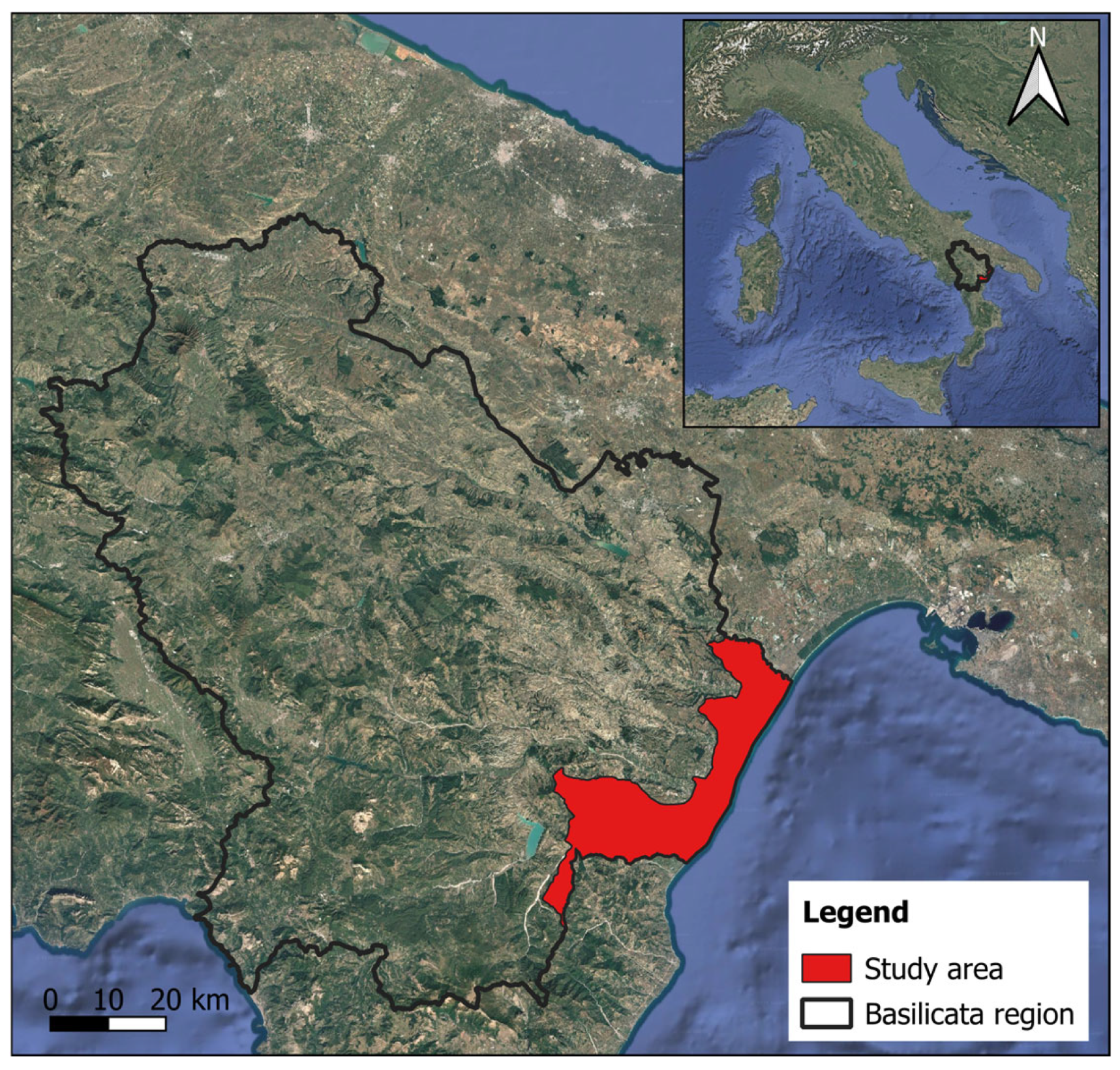
Disclaimer/Publisher’s Note: The statements, opinions and data contained in all publications are solely those of the individual author(s) and contributor(s) and not of MDPI and/or the editor(s). MDPI and/or the editor(s) disclaim responsibility for any injury to people or property resulting from any ideas, methods, instructions or products referred to in the content.

Article Metrics

Citations

Article Access Statistics

Multiple requests from the same IP address are counted as one view.