Regional Soil Erosion Assessment Using Remote Sensing and Field Validation: Enhancing the Erosion Potential Model

Highlights

What are the main findings?

• A two-stage framework integrating the Erosion Potential Model (EPM) with multi-temporal Landsat-derived indices (NDVI and BSI) and systematic field calibration significantly enhanced model performance (AUC: 0.820 to 0.854; Overall Accuracy: 0.78 to 0.84; F1-score: 0.78 to 0.85).
• Remote sensing-based dynamic correction of land cover protection (X·a) and visible erosion (φ) parameters revealed substantial spatial redistribution of erosion intensity, with a 30.37% expansion of medium-to-excessive classes and an increase in the mean erosion coefficient (Z: 0.21 to 0.24).

What is the implication of the main finding?

• The integration of spectral indices with empirical erosion modeling reduces uncertainty in regional-scale assessments and improves discrimination of erosion-prone surfaces in heterogeneous mountainous environments.
• The field-validated framework provides a transferable and operational methodology for sediment yield estimation and spatial prioritization of soil conservation measures across large (26,570 km²) data-limited regions.

Abstract

Soil erosion assessment in Southeast Europe’s mountainous regions often lacks systematic field validation, limiting confidence in model-based predictions. This study integrates the Erosion Potential Model (EPM) with remote sensing and field verification across 26,570 km² in the Federation of Bosnia and Herzegovina (FBiH) and Brčko District (BD). We developed a two-stage framework: initial GIS-based assessment using digital elevation models, soil maps, climate data, CORINE Land Cover, and Landsat imagery, followed by field calibration at 190 representative sites. Spectral indices (NDVI, BSI) provided dynamic corrections for vegetation cover and visible erosion features. Field validation significantly improved model performance; the erosion coefficient increased from Z = 0.21 to Z = 0.24, while discriminatory power improved AUC from 0.82 to 0.85, with corresponding gains in overall accuracy from 0.78 to 0.84 and F1-score from 0.78 to 0.85. The field-validated model estimated mean annual sediment production of 546.60 m³·km⁻²·year⁻¹, with total erosion material production of 14,074,940.2 m³·year⁻¹. Field calibration revealed substantial spatial redistribution, with medium-to-excessive erosion categories expanding by 30.37%, affecting 1319.12 km² requiring priority intervention. The Kappa coefficient (0.81) confirms high classification reliability. This field-validated framework enables evidence-based identification of degradation hotspots and provides actionable guidance for soil conservation planning in geomorphologically heterogeneous, data-limited regions.

1. Introduction

Soil erosion, recognized as one of the main drivers of land degradation worldwide, poses a significant challenge in Europe [1,2,3,4,5]. It is estimated that annual losses in agricultural productivity within the European Union due to pronounced soil erosion amount to approximately €1.25 billion [6]. In addition to water erosion, wind erosion poses a significant threat in arid and semi-arid regions of Europe, where strong winds can remove topsoil and organic matter, leading to desertification and a decline in agricultural productivity [7,8,9,10,11]. Water erosion is the dominant land degradation process in Europe, causing substantial damage to agricultural land, water resources, and ecosystem health. Furthermore, water erosion can trigger landslides and torrential floods, posing risks to human settlements and infrastructure [12]. Unlike general flash floods, torrential floods represent a distinct category of flood events driven by the rapid concentration of surface runoff and sediment-laden flow in steep torrent channels, characterized by strong coupling with hillslope erosion and sediment delivery processes. The ecological and economic impacts of soil erosion are significant and include reduced agricultural yields, increased water treatment costs, and damage to infrastructure. The implementation of comprehensive soil conservation measures, the improvement of sustainable land management practices, and adaptation to climate change impacts are crucial to mitigating the negative effects of water erosion and preserving the long-term stability and productivity of European landscapes [13,14,15].

Addressing soil erosion requires a multifaceted approach that integrates sustainable land management practices, soil conservation measures, and institutional and regulatory actions. Soil erosion assessment and monitoring are fundamental steps in tackling erosion-related issues [16]. Understanding the complex interactions between human activities, climate change, and natural processes is essential for accurately predicting future erosion trends [17]. To further enhance these predictions, erosion models integrated with Geographic Information Systems (GISs) are applied to identify erosion hotspots [18,19]. These methodologies are often complemented by remote sensing technologies, enabling comprehensive spatial and temporal analyses of land-use changes [17,20].

Modeling erosion processes represents a key aspect of land resource management, particularly in areas prone to intensive land degradation. Traditional empirical models, such as the Erosion Potential Model (EPM) [21,22], enable quantification of soil loss based on several input factors and account for various erosion processes (ranging from sheet and rill erosion to gullies and mass movements) [16,23,24,25,26]. The EPM represents an empirical method for estimating soil loss, erosion production, and sediment yield within a catchment or a defined area. In addition to calculating sediment production and transport, the method was also developed for mapping erosion processes and erosion-prone areas, as well as for the quantitative classification of torrential streams [21,22,23,24]. Since its development, the method has undergone several modifications and has been widely applied—across all former Yugoslav republics [27,28,29,30,31,32,33,34,35], as well as internationally in Germany [36], Italy [37,38,39], Greece [26,40,41], Morocco [42], Brazil [43,44], and several other countries [45,46,47,48,49,50], and has been evaluated in global erosion assessments [16].

Despite its widespread application, the EPM presents certain challenges when applied at the regional scale. Its semi-empirical and deterministic nature relies on a limited set of input coefficients that are traditionally assigned using static tabular values based on qualitative field descriptions, which introduces subjectivity and uncertainty in parameter estimation across spatially heterogeneous areas. Furthermore, the φ coefficient, representing visible erosion processes, is inherently difficult to quantify consistently over large territories without systematic field surveys or remote sensing support. Compared to other widely used erosion models, such as the Revised Universal Soil Loss Equation (RUSLE) [51], EPM offers several advantages that make it particularly suitable for the study area. Unlike RUSLE, which is primarily designed to estimate sheet and rill erosion on agricultural land, EPM accounts for a broader range of erosion processes, including gully erosion, mass movements, and mixed erosion types, which are characteristic of the complex mountainous terrain of Bosnia and Herzegovina [52]. Moreover, EPM provides an integrated estimate of both erosion intensity and sediment yield at the catchment or regional scale, directly applicable to water management planning and torrential flood risk assessment, and has been institutionally adopted as the standard engineering tool across the former Yugoslav republics [21,22,24]. The territory of the Federation of Bosnia and Herzegovina (FBiH) and the Brčko District (BD) exemplifies the conditions under which such a framework is critically needed; complex geomorphology, rugged relief, heterogeneous land cover, and high hydro-meteorological variability make erosion processes, along with associated torrential floods and landslides, a significant socio-economic and environmental issue [52]. Catastrophic events in May 2014 caused damages exceeding €555.2 million in the FBiH alone [53,54,55,56], while more recent floods in October 2024 resulted in dozens of fatalities and severe infrastructure losses across central and southern Bosnia [57,58,59,60].

Although the EPM has been widely applied across the Balkan region and beyond, systematic field validation at the regional scale remains scarce, and the dynamic correction of model parameters using remote sensing-derived spectral indices has not been sufficiently explored. This study addresses these gaps by developing and applying a two-stage framework that integrates EPM with multi-temporal Landsat-derived NDVI and BSI indices, followed by systematic field calibration across 190 representative sites in the Federation of Bosnia and Herzegovina and Brčko District (26,570 km²). The methodological novelty of this study lies in the operational integration of spectral indices as dynamic correction tools for the land cover protection (X·a) and visible erosion (φ) coefficients, replacing static tabular assignments with spatially continuous, remotely sensed estimates. The expected contribution is threefold: (i) a field-validated regional soil erosion map with demonstrated improvement in classification performance; (ii) quantification of the added value of field calibration relative to desk-based modeling; and (iii) a transferable and operationally applicable framework for data-limited mountainous regions in Southeast Europe.

2. Materials and Methods

2.1. Study Area

The Federation of Bosnia and Herzegovina (FBiH) and the Brčko District (BD), together with the Republika Srpska (RS), constitute the state of Bosnia and Herzegovina (BiH), which is located in Southeast Europe and geographically belongs to the Adriatic and Black Sea watersheds, i.e., to the group of Mediterranean and Danubian countries.

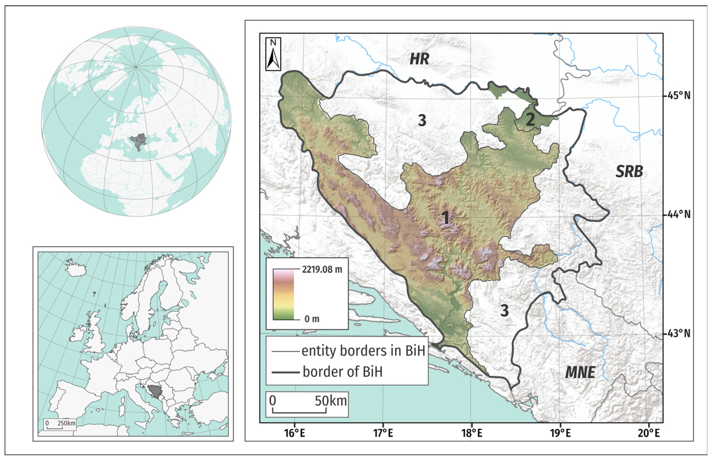
Bosnia and Herzegovina is situated in the central part of the Balkan Peninsula (Figure 1), between 42°26′ and 45°15′ north latitudes and 15°45′ and 19°41′ east longitudes. The total area of Bosnia and Herzegovina is 51,209.2 km², while the study area comprising FBiH and BD covers 26,570 km². The relief of BiH is predominantly hilly and mountainous, but at the same time highly dissected by lowland areas along major rivers. Of the total land area, 5% consists of plains, 24% hills, 42% mountains, and 29% karst fields [61]. Owing to its specific geographical position and relief, the climate of BiH is highly complex. Three distinct climatic zones can be identified, with more or less pronounced boundaries: the Mediterranean (maritime) climate in the southwest, the continental mountain (Alpine) climate in the central part, and the temperate continental (Central European) climate in the north [62].

The geological structure of Bosnia and Herzegovina is the result of a long history of geological activity. It is extremely complex, characterized by the formation of diverse rock types, including igneous, sedimentary, metamorphic, and numerous transitional forms. The most widespread lithological units in BiH are schists, followed by limestones and dolomites, and flysch–ophiolitic complexes [62].

The geological structure and climatic conditions have led to the development of various soil types, among which Calcomelanosols, Dystric Cambisols, and Calcic Cambisols are the most widespread in hilly and mountainous areas. Among automorphic soil types in these regions, Lithosols, Regosols, Terra rossa, Rendzinas, Luvisols, Podzols, and Vertisols are represented. In lowland areas, several hydromorphic soils occur, with Pseudogley and Fluvisols being the most prevalent [63]. According to CORINE Land Cover 2018 datasets [64], the most recent version available at the time of this study, most of BiH’s territory is covered by forests (53.2%), while agricultural land accounts for 26.8%. Urban and transport areas together occupy 1.7% of the total land area. Within forest land, broadleaved forests cover 32.62% of the territory, while coniferous and mixed forests account for 13.72%. Transitional woodland–shrub areas cover 5.53% of the territory, and land predominantly used for agriculture, with significant areas of natural vegetation, covers 8.65%. Agricultural land includes pastures, which account for 6.33% of the area, with various types of production (plantations, orchards, berry plantations, annual crops, intensive orchards, and vineyards) [61].

2.2. Data Sources and Preparation

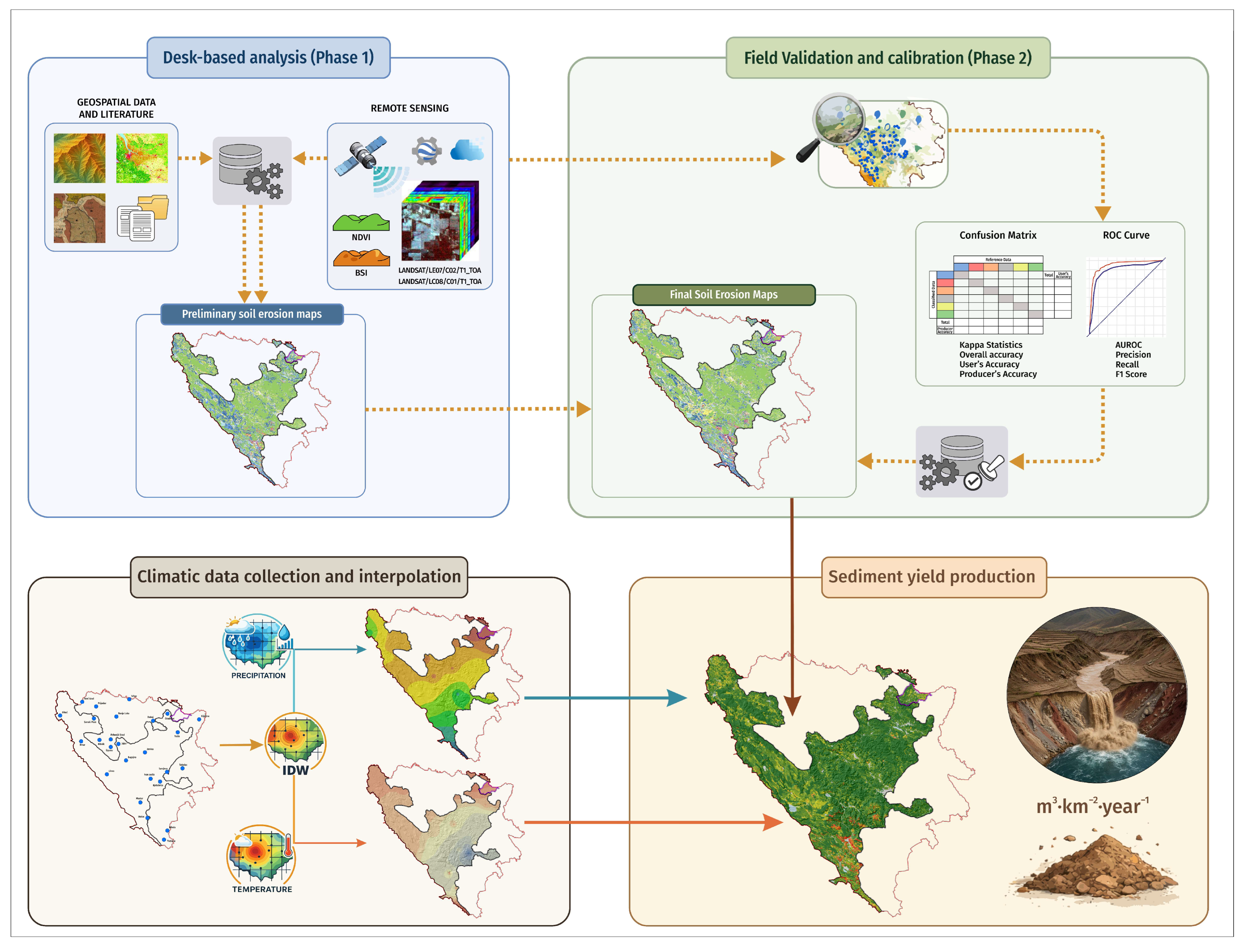
To apply the Erosion Potential Method (EPM) model to the study area of the FBiH and BD, all relevant input datasets were used to quantify the erosion coefficient (Z) and calculate sediment production (Figure 2). These datasets included spatial data in both raster and vector formats, along with associated metadata, which were integrated and analyzed using ArcMap 10.8 software [65]. Satellite-derived products were generated using the Google Earth Engine (GEE) platform [66] (

Table 1. Overview of spatial datasets used in the EPM application, including data type, spatial resolution, temporal coverage, and data source.

Data	Type	Description	Resolution	Duration	Source
Annual precipitation data	Vector and raster	Meteorological station network; station coordinates used as input points for IDW spatial interpolation to generate continuous raster surfaces	100 m	2010–2020	[67,68,69]
Annual temperature data	Vector and raster	Meteorological station network; station coordinates used as input points for IDW spatial interpolation to generate continuous raster surfaces	100 m	2010–2020	[67,68,69]
Digital elevation model	Raster	EU-DEM v1.1, Copernicus Land Monitoring Service	25 m	2015	[70]
Land Cover map	Vector	CORINE Land Cover 2018	100 m	2018	[64]
Soil map	Vector	Basic Soil Map of Bosnia and Herzegovina, 116 map sheets, georeferenced and digitized	Scale 1:50,000	1960–1980	[63]
Normalized Vegetation Index (NDVI)	Raster	LANDSAT/LE07/C02/T1_TOA and LANDSAT/LC08/C01/T1_TOA	30 m	1 January 2010–31 December 2020.	[71]
Bare Soil Index (BSI)	Raster	LANDSAT/LE07/C02/T1_TOA and LANDSAT/LC08/C01/T1_TOA	30 m	1 January 2010–31 December 2020.	[71]

).

The primary task in developing the soil erosion map was establishing a geodatabase, which serves as the fundamental informational and geometric framework for relevant spatial datasets. The geodatabase comprises the key factors influencing the occurrence and development of soil erosion processes. Its creation represents an initial step toward the development of a progressively operational database that, among other purposes, serves as a foundation for preparing field investigation activities. The formation of the geodatabase was a complex process involving the collection, digitization, and harmonization of relevant datasets (vector data, raster data, and metadata), which required both spatial and informational adjustment within a GIS (Geographic Information System) environment.

One favorable circumstance was the availability of global and European-level datasets that could be applied to the study area with a certain level of accuracy. All datasets were standardized to the MGI/Balkans 6 coordinate reference system (EPSG: 31276). This system is based on the Gauss–Krüger projection, using the Bessel 1841 ellipsoid and a defined central meridian of 18° east of Greenwich.

Climate data were obtained from 26 meteorological stations distributed across the study area and surrounding region, maintained by the Federal Hydrometeorological Institute of Bosnia and Herzegovina (FHMZBIH) [67], and the Republic Hydrometeorological Institute of Republika Srpska (RHMZRS) [69] which continuously measures and publishes climatological time series through the national meteorological station network. The United Nations Framework Convention on Climate Change (UNFCCC), which reports average annual air temperatures and precipitation amounts for different regions of the country [68], provided the additional context regarding the climatic characteristics of the study area. Inverse Distance Weighted (IDW) interpolation method generated the spatial distribution of climatic variables across the study area [72] (see Supplementary Figures S1 and S2). The IDW method was selected due to its computational simplicity, deterministic nature, and suitability for the available station density in the study area. Although geostatistical methods such as ordinary kriging can provide superior interpolation accuracy when the spatial autocorrelation of climatic variables is well-defined, their application requires a sufficient number of observation points to reliably estimate the variogram. Given the uneven spatial distribution of meteorological stations across the complex relief of BiH, IDW was deemed the most robust and reproducible approach for this application.

The Basic Soil Map of Bosnia and Herzegovina at a scale of 1:50,000, produced by the Institute for Agropedology in Sarajevo as part of a national soil mapping project conducted between 1960 and 1980 [63], provided the pedological basis for the study. The physical and mechanical properties of soils were interpreted based on this map, accompanying soil survey documentation, and relevant pedological literature. This approach provided data on soil types and subtypes, texture, profile depth, structure, permeability, and soil erodibility. These data were used to determine the soil resistance coefficient to erosion (Y) within the EPM framework.

The digital elevation model from the pan-European EU-DEM database, with a 25 m spatial resolution, was used for terrain analysis and slope modeling [70]. CORINE Land Cover (CLC) dataset, a standardized European land cover database with a 100 m spatial resolution, provided data on land cover and land use within the study area [64].

Landsat satellite imagery from missions 7 and 8, with a spatial resolution of 30 m, was used to analyze erosion processes. The official website of the United States Geological Survey (USGS) [71] via the Google Earth Engine (GEE) platform [66] provided the imagery. Landsat imagery used to develop the soil erosion map covered 10 years from 1 January 2010 to 31 December 2020. Satellite scenes with the lowest cloud cover were selected for each month. To ensure the relevance of results, imagery from both vegetation and non-vegetation periods was used. Before data acquisition, digital image processing was performed, including geometric, atmospheric, and radiometric corrections [73,74].

Following primary image processing, products derived from available spectral bands were generated as spectral indices. Used spectral indices included the Normalized Difference Vegetation Index (NDVI) [75] and the Bare Soil Index (BSI) [76]. The NDVI was used to identify vegetation cover and to correct input parameters for soil erosion calculation. In addition to NDVI (see Supplementary Figure S3), the BSI was applied (see Supplementary Figure S4) to detect visible erosion processes and identify urbanized and impervious surfaces. The BSI was likewise used to correct input parameters for soil erosion estimation.

It is acknowledged that resampling all spatial datasets to a common 100 m resolution, while necessary for methodological consistency with the CORINE Land Cover dataset, introduces a degree of spatial generalization that may affect the accuracy of derived parameters. In particular, the EU-DEM, originally at 25 m resolution, and Landsat imagery at 30 m were both upscaled to 100 m, which results in a smoothing of terrain gradients and a reduction in the range of slope values. This spatial averaging tends to suppress local maxima in the mean slope coefficient (I_mean), potentially leading to an underestimation of the erosion coefficient (Z) in highly dissected terrain and steep mountain slopes, including karst areas. Similarly, the 100 m resolution limits the detection of fine-scale vegetation heterogeneity captured by NDVI, which may reduce the sensitivity of the X·a coefficient in transitional land cover zones. The potential underestimation of erosion intensity in topographically complex areas should therefore be considered when interpreting results at sub-regional or local scales, and higher-resolution analyses are recommended for local-scale management applications. Nevertheless, the selected resolution is consistent with the spatial detail of the primary land cover input (CORINE Land Cover, 100 m), appropriate for the strategic planning purposes of this regional-scale assessment, and in line with comparable regional EPM studies conducted across Southeast Europe.

2.3. Erosion Potential Method (EPM)

The EPM is an empirical method for assessing soil loss, erosion production, and sediment transport in a watershed, erosion area, or land parcel. This technique was developed based on long-term field research, observations, and watershed measurements [21,22]. In addition to calculating sediment production and transport, this method was designed for mapping and assessing erosion processes in erosion-prone areas and quantitatively classifying torrential flows [21,23,24]. This method is a standard tool for solving engineering problems related to preventing soil erosion and torrential floods in water management. To develop water management foundations, studies, and projects, Equations (1) and (2) is used [21]:

$$\mathrm{W}=\mathrm{T}·{\mathrm{H}}_{\mathrm{y}\mathrm{e}\mathrm{a}\mathrm{r}}·\mathsf{\pi }·\sqrt{{\mathrm{Z}}^3}·\mathrm{A}$$

(1)

W—Total production of erosive material (i.e., annual gross erosion) [m³∙year⁻¹]; T—temperature coefficient [-]; H_year—mean annual precipitation [mm]; π—3.14; Z—coefficient of erosion [-]; A—watershed area [km²].

$${\mathrm{W}}_{\mathrm{s}\mathrm{p}}={\displaystyle \frac{\mathrm{W}}{A}}$$

(2)

W_sp—specific annual production of erosive material (i.e., specific annual gross erosion) [m³∙km²∙year⁻¹].

The temperature coefficient of the area is calculated according to Equation (3) [21]:

$$\mathrm{T}=\sqrt{{\displaystyle \frac{\mathrm{t}}{10}}+0.1}$$

(3)

t—average annual air temperature in the research area [°C].

The method starts with the analytical processing of data on factors influencing erosion. Since erosion is a spatial phenomenon, it is represented on maps based on classification according to the analytically calculated erosion coefficient (Z), which is not dependent on climatic characteristics but on soil characteristics, vegetation cover, relief, and the visible occurrence of erosion processes. The erosion coefficient (Z) is obtained from Equation (4) [21]:

$$\mathrm{Z}=\mathrm{Y}·\mathrm{X}·\mathrm{a}·\left(\mathsf{\phi }+\sqrt{{\mathrm{I}}_{\mathrm{m}\mathrm{e}\mathrm{a}\mathrm{n}}}\right)$$

(4)

Z—erosion coefficient [-]; Y—soil erodibility coefficient (soil resistance to erosion) [-]; X∙a—soil protection coefficient (land use and land cover) [-]; φ—coefficient of type and extent of erosion and slumps [-]; ${\mathrm{I}}_{\mathrm{m}\mathrm{e}\mathrm{a}\mathrm{n}}$—the mean slope coefficient [%].

Based on the erosion coefficient (Z), erosion processes can be categorized according to the work by Gavrilović (

Table 2. Classification of the erosion classes according to the Z coefficient [21].

Erosion Class	Intensity of Erosion Processes	Dominant Erosion Type	Erosion Coefficient Z	Mean Value of Z
I	Excessive erosion	Deep	>1.51	1.25
		Mixed	1.21–1.50
		Surface	1.01–1.20
II	Severe erosion	Deep	0.91–1.00	0.85
		Mixed	0.81–0.90
		Surface	0.71–0.80
III	Medium erosion	Deep	0.61–0.70	0.55
		Mixed	0.51–0.60
		Surface	0.41–0.50
IV	Slight erosion	Deep	0.31–0.40	0.30
		Mixed	0.25–0.30
		Surface	0.20–0.24
V	Very slight erosion	Traces of erosion	0.01–0.19	0.10

). The values typically range from 0.1 to 1.5 and higher, i.e., from preserved, mildly eroded catchments and areas to catchments significantly degraded due to soil erosion. Z values may only be above and below the mentioned thresholds in exceptional cases [24]. Thirteen categories have been established based on the type of prevailing erosion and the values of the erosion coefficient (Z) (Table 2) [21].

The soil erodibility coefficient (Y) depends on the climatic conditions of the environment, geological substrate, and types of pedological formations being analyzed. According to the original method, the values of the coefficient range from 0.25 for bare and compact rocks to 2.0 for fine sediments and unbound soils without the ability to resist erosion [21] (see Supplementary Table S1). The values of the Y coefficient for the territory of the FBiH and BD were defined based on a digitized pedological map at a scale of 1:50,000.

The soil protection coefficient (X∙a) relates to the soil’s protection from atmospheric agents and erosion effects. This coefficient comprises the original or ‘unchanged’ land cover (‘X’) and soil protection measures (‘a’). According to Gavrilović, its values range from 0.05 to 1.0 (see Supplementary Table S2) [21]. The soil protection coefficient (X·a) was determined by overlaying the multi-temporal Landsat-derived NDVI raster (computed using Equation (5)) with the CORINE Land Cover vector dataset. Each CLC polygon was treated individually, with the mean NDVI value extracted for that specific polygon serving as the basis for X·a assignment. This approach follows a logic analogous to the NDVI-based derivation of the RUSLE C-factor [4], in which higher NDVI values, indicative of dense and continuous vegetation cover, correspond to lower X·a values reflecting greater soil protection, while lower NDVI values within the same land cover class indicate degraded or sparse vegetation and were assigned proportionally higher X·a values. This polygon-level approach avoids the use of uniform class-average values and instead captures the spatial variability of vegetation protective capacity within each land cover category, in accordance with the original EPM coefficient ranges defined by Gavrilović [21].

$$\mathrm{N}\mathrm{D}\mathrm{V}\mathrm{I} = {\displaystyle \frac{\mathrm{N}\mathrm{I}\mathrm{R} - \mathrm{R}\mathrm{E}\mathrm{D}}{\mathrm{N}\mathrm{I}\mathrm{R} + \mathrm{R}\mathrm{E}\mathrm{D}}}$$

(5)

NIR—near-infrared spectral channels; RED—red spectral channels.

The I_mean coefficient represents the topographic characteristics of the study area and describes the general relief conditions and geomorphological features. According to the EPM, the mean slope is expressed as a weighted arithmetic mean of the areas between two contour lines [21]. This value was derived from a digital elevation model with a spatial resolution of 100 m, using slope-generation tools in a GIS environment.

The coefficient of the types and extent of erosion and slumps (φ) represents the numerical equivalent of visible and clearly expressed erosion processes in a watershed or erosion area (see Supplementary Table S3). The coefficient of type and extent of erosion and slumps (φ) was derived from the Bare Soil Index (BSI) through linear min–max normalization, as described in Equation (6) [77]. The BSI composite was computed from all available cloud-free Landsat scenes acquired during the 10-year study period (2010–2020), ensuring a temporally representative characterization of bare-soil exposure across the study area. Before the normalization procedure, urban areas, water bodies, and wetlands were excluded from the analysis through spatial masking, thereby reducing the risk of misclassifying spectrally similar impervious or water surfaces as erosion-prone bare soil. The resulting normalized BSI values were linearly rescaled to the φ range (0.1–1.0), where maximum BSI values representing bare soil and rock surfaces correspond to φ = 1.0, and minimum BSI values associated with dense vegetation correspond to φ = 0.1, consistent with the original EPM coefficient boundaries [21].

$$\mathsf{\phi } = {\displaystyle \frac{\mathrm{B}\mathrm{S}\mathrm{I} - {\mathrm{B}\mathrm{S}\mathrm{I}}_{\mathrm{m}\mathrm{i}\mathrm{n}}}{{\mathrm{B}\mathrm{S}\mathrm{I}}_{\mathrm{m}\mathrm{a}\mathrm{x}} - {\mathrm{B}\mathrm{S}\mathrm{I}}_{\mathrm{m}\mathrm{i}\mathrm{n}}}}$$

(6)

φ—The coefficient of type and extent of erosion; BSI—the bare soil index; BSI_max—a value representing bare soil in the BSI layer; BSI_min—a value representing vegetation in the BSI layer.

The BSI values range from −1 to +1, where positive values indicate a higher presence of bare soil and impervious surfaces, while negative values reflect the presence of vegetation and porous surfaces. This linear transformation assumes that maximum BSI values (bare soil/rock) correspond to surfaces with visible erosion features (φ = 1), while minimum BSI values (dense vegetation) indicate erosion-free areas (φ = 0.1). The BSI values were computed using Equation (7) [76,78].

$$\mathrm{B}\mathrm{S}\mathrm{I} = {\displaystyle \frac{\left(\mathrm{S}\mathrm{W}\mathrm{I}\mathrm{R} + \mathrm{R}\mathrm{E}\mathrm{D}\right) - (\mathrm{N}\mathrm{I}\mathrm{R} + \mathrm{B}\mathrm{L}\mathrm{U}\mathrm{E})}{\left(\mathrm{S}\mathrm{W}\mathrm{I}\mathrm{R}+\mathrm{R}\mathrm{E}\mathrm{D}\right) + (\mathrm{N}\mathrm{I}\mathrm{R} + \mathrm{B}\mathrm{L}\mathrm{U}\mathrm{E})}}$$

(7)

SWIR—shortwave infrared spectral channels; RED—red spectral channels; NIR—near-infrared spectral channels; BLUE—blue spectral channels.

This innovative approach for deriving the coefficient of visible and clearly expressed erosion processes has been successfully applied in hilly–mountainous catchments in Serbia [79], in the Sarajevo Canton [80], as well as in mountainous catchments in Greece [26].

2.4. Models Validation and Accuracy Assessment

2.4.1. ROC Curve and AUC Value

For the quantitative assessment of the predictive performance of soil erosion maps, Receiver Operating Characteristic (ROC) analysis and the corresponding Area Under the Curve (AUC) values were employed. The ROC curve illustrates the relationship between the true positive rate and the false positive rate across different classification thresholds, enabling the evaluation of the model’s ability to discriminate between erosion-prone areas and stable surfaces. The AUC represents the area under the ROC curve and serves as a numerical indicator of model reliability, where values closer to 1 indicate high discriminative capability, while values around 0.5 suggest random prediction [81]. The analysis was applied to erosion maps derived from both the desk-based and field-validation phases, using a binary approach for the independent evaluation of each class. In addition to ROC/AUC analysis, model performance was evaluated using standard statistical metrics: true positive rate (TPR) (Equation (8)), false positive rate (FPR) (Equation (9)), AUROC (Equation (10)), overall accuracy (Equation (11)), precision (Equation (12)), recall (Equation (13)), and F1-score (Equation (14)). The true positive rate (TPR) and false positive rate (FPR) were used to construct the ROC curve, while AUROC provides a comprehensive indicator of the model’s discriminative power. Overall accuracy reflects the proportion of correctly classified samples, precision measures the proportion of correctly predicted erosion locations, recall evaluates the model’s ability to detect truly erosion-affected areas, and the F1-score represents the harmonic mean of precision and recall. The F1-score is particularly relevant under conditions of class imbalance, which are common in erosion-related studies [82,83].

$$\mathrm{T}\mathrm{P}\mathrm{R} = {\displaystyle \frac{TP}{TP + FN}}$$

(8)

$$\mathrm{F}\mathrm{P}\mathrm{R} = {\displaystyle \frac{FP}{FP + TN}}$$

(9)

$$\mathrm{A}\mathrm{U}\mathrm{R}\mathrm{O}\mathrm{C} = {\sum }_{i=1}^{n-1}({FPR}_{i+1} - {FPR}_i)·({\displaystyle \frac{{TPR}_{i+1} + {TPR}_i}{2}})$$

(10)

$$\mathrm{O}\mathrm{v}\mathrm{e}\mathrm{r}\mathrm{a}\mathrm{l}\mathrm{l} \mathrm{A}\mathrm{c}\mathrm{c}\mathrm{u}\mathrm{r}\mathrm{a}\mathrm{c}\mathrm{y}={\displaystyle \frac{TP + TN}{TP + TN + FP + FN}}$$

(11)

$$\mathrm{P}\mathrm{r}\mathrm{e}\mathrm{c}\mathrm{i}\mathrm{s}\mathrm{i}\mathrm{o}\mathrm{n}={\displaystyle \frac{TP}{TP + FP}}$$

(12)

$$\mathrm{R}\mathrm{e}\mathrm{c}\mathrm{a}\mathrm{l}\mathrm{l}={\displaystyle \frac{TP}{TP + FN}}$$

(13)

$$F_{1 } \mathrm{s}\mathrm{c}\mathrm{o}\mathrm{r}\mathrm{e} = 2 · {\displaystyle \frac{Precision · Recall}{Precision + Recall}}$$

(14)

2.4.2. Confusion Matrix and Model Accuracy Evaluation

To assess the accuracy of soil erosion maps produced using the EPM approach, a confusion matrix–based analysis was applied. This metric enables the quantification of agreement between erosion classes predicted by the model and the actual field conditions, the identification of correctly and incorrectly classified locations, as well as the comparison of maps derived from the desk-based and field-validation phases, thereby allowing the contribution of fieldwork to improvements in model accuracy to be evaluated. The confusion matrix provides the basis for deriving various accuracy measures, including overall accuracy (Equation (15)), user’s accuracy (Equation (16)), producer’s accuracy (Equation (17)), and the Kappa statistic (Equation (18)) [74,84,85,86,87,88]. Overall accuracy expresses the proportion of correctly classified locations and reflects the general reliability of the model. Producer’s accuracy measures the ability of the model to correctly identify actual erosion classes, whereas user’s accuracy indicates the probability that a location classified as erosion-prone indeed belongs to that class. In addition to these basic metrics, the Kappa statistic was employed to account for chance agreement and to provide a more rigorous assessment of classification accuracy. Kappa coefficient values closer to 1 indicate high agreement, while values below 0.4 suggest low classification reliability [74,84].

$$\mathrm{O}\mathrm{A}={\displaystyle \frac{{\sum }_{\mathrm{i}=1}^{\mathrm{r}}{\mathrm{x}}_{\mathrm{i}\mathrm{i}}}{\mathrm{N}}}$$

(15)

$${\mathrm{P}\mathrm{A}}_{\mathrm{i}}={\displaystyle \frac{{\mathrm{x}}_{\mathrm{i}\mathrm{i}}}{{\mathrm{x}}_{+\mathrm{i}}}}$$

(16)

$${\mathrm{U}\mathrm{A}}_{\mathrm{i}}={\displaystyle \frac{{\mathrm{x}}_{\mathrm{i}\mathrm{i}}}{{\mathrm{x}}_{\mathrm{i}+}}}$$

(17)

$$\mathrm{K}\mathrm{a}\mathrm{p}\mathrm{p}\mathrm{a}={\displaystyle \frac{\mathrm{N}{\sum }_{\mathrm{i}=1}^{\mathrm{r}}{\mathrm{x}}_{\mathrm{i}\mathrm{i}}-{\sum }_{\mathrm{i}=1}^{\mathrm{r}}{(\mathrm{x}}_{\mathrm{i}+}·{\mathrm{x}}_{+\mathrm{i}})}{{\mathrm{N}}^2-{\sum }_{\mathrm{i}=1}^{\mathrm{r}}{(\mathrm{x}}_{\mathrm{i}+}·{\mathrm{x}}_{+\mathrm{i}})}}$$

(18)

where r denotes the number of rows in the matrix; X_ii represents the number of samples in row i and column i (i.e., the diagonal elements of the matrix); X_i+ denotes the sum of row i; X_+i denotes the sum of column i; and N is the total number of samples.

2.4.3. Correlation Analysis

Pearson’s correlation coefficient (r) assesses both the strength and the direction of the linear relationship between two variables. In this study, Pearson correlation analysis was conducted to examine the relationships between the specific annual production of eroded material (W_sp), erosion coefficient (Z), and the input parameters that potentially influence the occurrence of erosion processes. Pearson’s correlation coefficient (r) is calculated as follows [89] (Equation (19)):

$$r={\displaystyle \frac{\sum (x_i-\overline{x})·(y_i-\overline{y})}{\sqrt{{\sum {(x_i-\overline{x})}^2·\sum (y_i-\overline{y})}^2}}}$$

(19)

where xi and yi represent the values of variables x and y in the i-th sample, $\overline{x}$ and $\overline{y}$ denote the mean values of variables x and y, n is the sample size.

2.4.4. Descriptive Statistical Analysis

In addition to correlation analysis, an analytical–descriptive data processing approach was applied using box-plot diagrams. Box plots were employed to provide a graphical interpretation of the variability in erosion material production across different land cover types, as well as to illustrate the distribution of erosion values within individual categories. The box-plot diagram represents data distributions through key statistical descriptors, including minimum and maximum values, the median, the interquartile range (IQR), and potential outliers. This approach allows clear identification of differences among land cover types in terms of their susceptibility to generating eroded material. Land cover types exhibiting higher medians and wider interquartile ranges indicate a higher degree of erosion instability, whereas those with narrower distributions and lower values represent more stable surfaces.

2.5. Field Survey Work

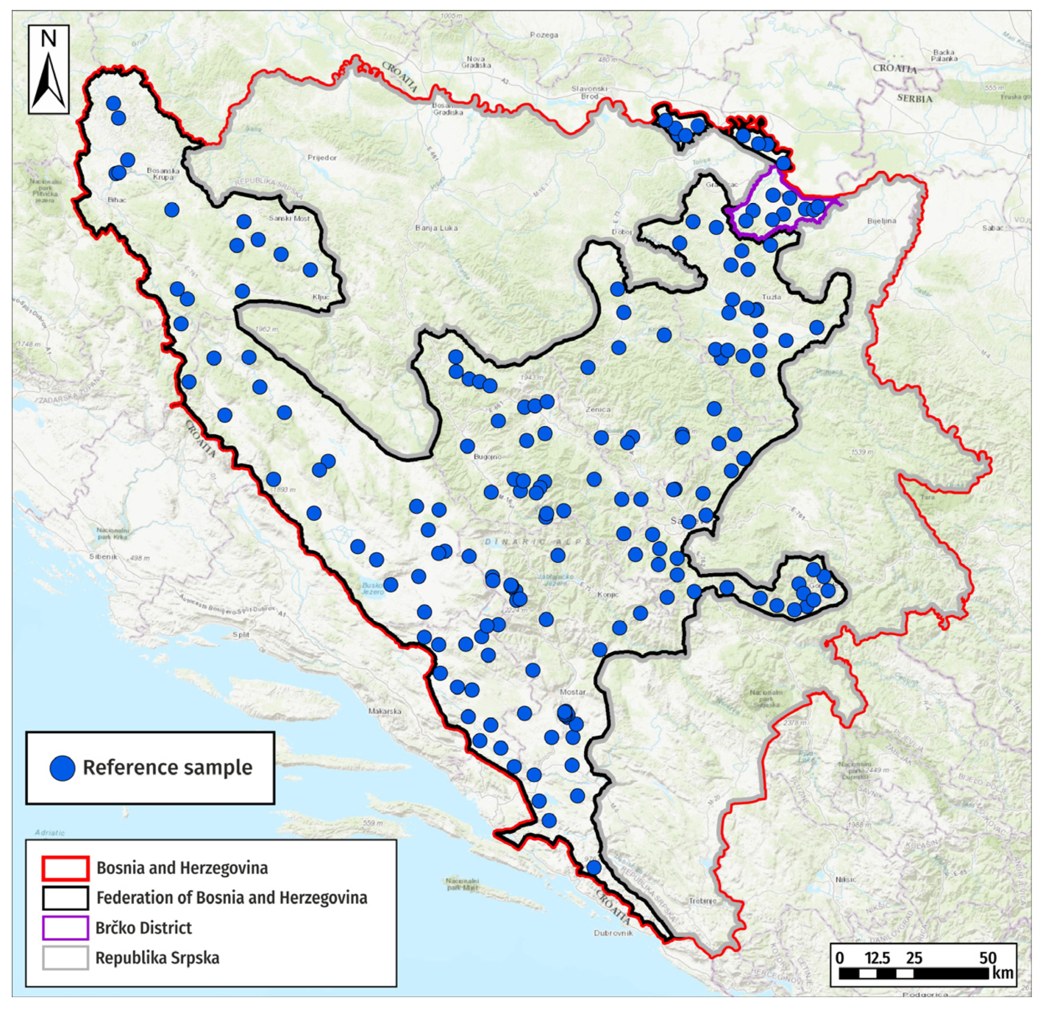
The desk-based (Phase 1) soil erosion database represents a key phase following the establishment of the geodatabase and serves as the basis for planning field survey activities. At this stage, the soil erosion coefficient (Z) was calculated using Equation (4). The desk-based soil erosion map was generated in a GIS environment, with the Z coefficient represented as a raster at a 100 m spatial resolution. The analysis was conducted exclusively in areas susceptible to erosion, including agricultural land, forested and grassland areas, shrub vegetation, and semi-natural landscapes. In contrast, urbanized areas, water bodies, and wetlands were excluded from the analysis because they lack a soil layer [5]. Visible erosion indicators recorded during field surveys included: surface sheet erosion and inter-rill erosion features, rill and ephemeral gully development, permanent gully erosion, mass movement features (shallow landslides and soil slumps), sediment deposition at slope bases and in channel beds, as well as the condition of vegetation cover and land-use practices. These observations were systematically recorded on standardized field forms accompanied by georeferenced photographic documentation. These data were used to calibrate input parameters and validate the results of the desk-based soil erosion map, thereby ensuring greater reliability of the field-validated soil erosion map. Calibration of input parameters involved the systematic comparison of desk-based EPM coefficient values (X·a and φ) with field-observed conditions at each survey location. Where significant discrepancies were identified between the model-assigned coefficient class and the field-verified erosion intensity, the relevant coefficient values were adjusted within the bounds prescribed by the original EPM methodology. Adjustments to the X·a coefficient reflected observed vegetation cover density, land-use intensity, and soil surface protection status, while φ corrections accounted for the presence, type, and spatial extent of visible erosion features identified in the field. The selection of field survey locations was based on the spatial representation of erosion categories, as well as terrain accessibility and safety constraints (e.g., minefield zones, road infrastructure, protected areas, hydrographic networks, settlements, etc.). In total, 190 field locations were defined and evenly distributed across the territory of the FBiH and BD (Figure 3), with fieldwork conducted between June and December 2021.

Following completion of field surveys and data collection, the correction of the desk-based soil erosion geodatabase resulted in the production of the field-validated soil erosion geodatabase. The field-validated soil erosion geodatabase for the study area was produced by applying the analytical expression based on calibrated input parameters. The calibration of input parameters and the resulting changes in erosion intensity categories were analyzed using statistical metrics and accuracy assessments. Accuracy assessment is a key component and central focus of numerous studies that evaluate classification reliability. Fundamentally, accuracy assessment determines the quality of information derived from field surveys, remote sensing, laboratory investigations, and related approaches. These assessments may be qualitative or quantitative. Qualitative assessments involve comparing the obtained data with actual field conditions, whereas quantitative assessments aim to identify and quantify errors. In such evaluations, data from the derived thematic maps are compared with reference (ground truth) data collected through systematic field surveys.

3. Results

3.1. Comparative Analysis of Soil Erosion Maps

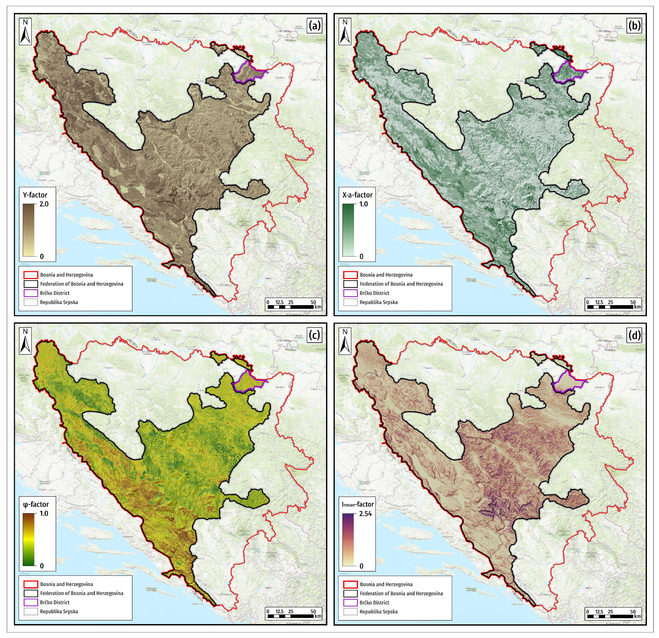
To assess the reliability of the EPM-based soil erosion model, a statistical analysis was conducted comparing results from the desk-based soil erosion map (Phase 1) with those from the field-validated soil erosion map produced after field investigations (Phase 2). This approach enabled the evaluation of the level of concurrence, deviations, and improvements in the model results relative to actual field conditions. Based on the established geodatabase and the conducted field surveys, calibrated input parameters for the calculation of the erosion coefficient (Z) were defined (Table S4 in the Supplementary Materials). The soil erodibility coefficient Y ranges from 0 to 2, with a mean value of 0.93 across the entire study area (Figure 4a). The soil protection coefficient X·a ranges from 0 to 1, with a mean value of 0.29 (Figure 4b). The coefficient of type and extent of erosion and slumps (φ) ranges from 0 to 1, with a mean value of 0.39 (Figure 4c). The mean slope coefficient (I_mean) has an average value of 0.21, with values ranging from 0 to 2.54 (Figure 4d).

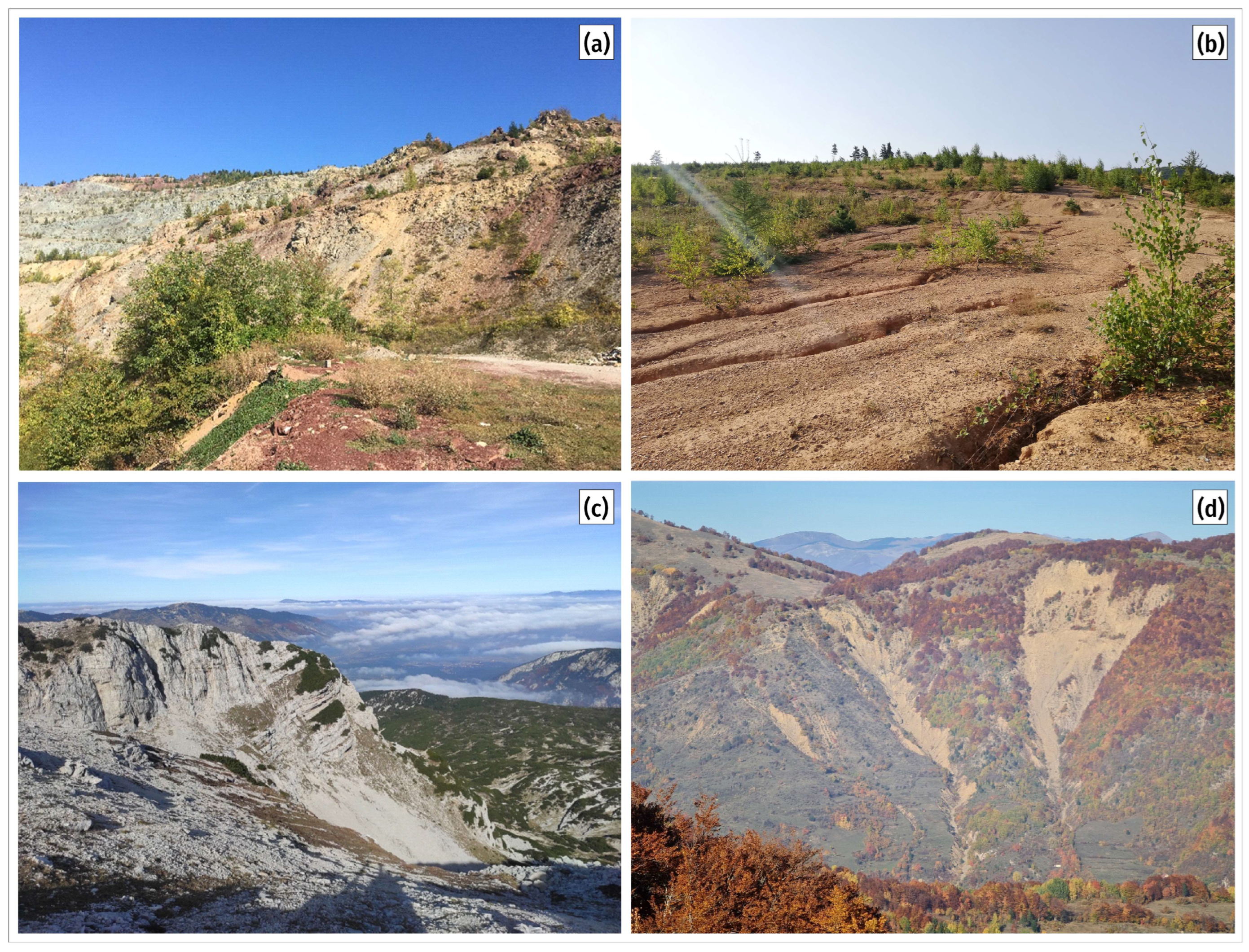
Field investigations included terrain reconnaissance and systematic field surveys, with detailed collection of relevant data on indicators associated with specific annual erosion categories, including visible erosion features, vegetation condition, land use practices, and land cover structure. These data were recorded in standardized field survey forms. Standardized field forms integrated preliminary GIS results with field-observable parameters (visible erosion features, vegetation condition, land use) necessary for model calibration. The field data collection included elements required for calibrating input parameters, such as visible evidence of erosion processes, land cover structure, and land use patterns (Figure 5).

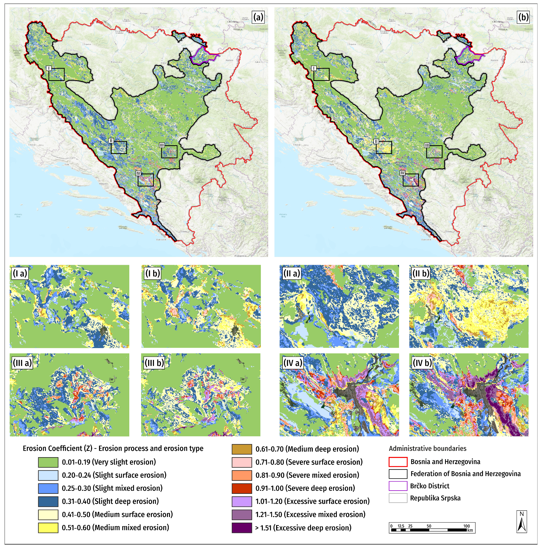
Field survey forms, together with accompanying photographic documentation, play a significant role in assessing the accuracy of the desk-based soil erosion map and correcting its input parameters and results, thereby providing quantitative guidance for the development of a representative field-validated soil erosion map. The selection of field survey locations was based on the distribution of soil erosion categories identified during the preparation of the desk-based map, as well as on available auxiliary data influencing fieldwork logistics, such as mine-contaminated areas, road infrastructure, protected zones, the hydrographic network, and settlement locations. Upon completion of field investigations and data collection, the desk-based (Phase 1) soil erosion map was corrected, resulting in the field-validated soil erosion map (Phase 2). The analysis of both the desk-based and field-validated soil erosion maps indicates the presence of all erosion intensity categories, ranging from very slight to excessive. The average erosion coefficient derived from the desk-based soil erosion map is Z_mean = 0.21, classifying the study area as slight erosion, with coefficient values ranging from Z = 0.01 to 2.49 (Figure 6a). After field verification, the average erosion coefficient increases to Z_mean = 0.24 (still within the slight erosion category), with values ranging from Z = 0.01 to 3.24 (Figure 6b).

Analysis of the desk-based soil erosion map (Phase 1) shows that the majority of the study area falls into the very slight and slight erosion categories. Very slight erosion covers an area of 14,566.11 km², representing 56.57% of the total territory, while slight erosion occupies 6840.08 km² (26.56%). Moderate erosion is recorded over 3797.66 km² (14.75%), whereas more intensive erosion processes are considerably less widespread, with severe erosion affecting 387.99 km² (1.51%) and excessive erosion covering 157.82 km² (0.61%) of the study area. After field investigations and calibration of input parameters, the field-validation soil erosion map (Phase 2) shows spatial redistribution of erosion intensity classes. The area affected by very slight erosion marginally decreases to 14,183.61 km² (55.08%), while slight erosion covers 5903.46 km² (22.93%), indicating a partial transition of some areas toward more intensive erosion categories. The most pronounced change is observed in the medium erosion category, which increases to 4820.87 km² (18.72%), reflecting the spatial expansion of zones with medium erosion intensity identified during field verification. Although intensive erosion categories remain proportionally the least represented, they exhibit greater spatial extent than in the desk-based phase. Areas affected by severe erosion increased to 476.19 km² (1.85%), while excessive erosion expanded to 365.53 km² (1.42%), representing more than a twofold increase compared to the desk-based results. These changes result from improvements in input spatial data, more accurate field identification of erosion features, and correction of model parameters based on observed conditions (see Supplementary Figures S5 and S6). The total area of the study region remains unchanged at 25,749.66 km² in both phases of the analysis. The obtained results confirm the importance of integrating desk-based modeling with field verification to achieve a reliable assessment of the spatial distribution and intensity of erosion processes (

Table 3. Erosion coefficient (Z) in the study area.

Erosion Class	Intensity of Erosion Processes	Erosion Coefficient (Z)	Desk Based Z (Phase 1)		Field Validation Z (Phase 2)
			km2	%	km2	%
I	Excessive erosion	>1.01	157.82	0.61	365.53	1.42
II	Severe erosion	0.71–1.00	387.99	1.51	476.19	1.85
III	Medium erosion	0.41–0.70	3797.66	14.75	4820.87	18.72
IV	Slight erosion	0.20–0.40	6840.08	26.56	5903.46	22.93
V	Very slight erosion	0.01–0.19	14,566.11	56.57	14,183.61	55.08
	Total		25,749.66	100	25,749.66	100

).

A more detailed examination of the four representative localities highlighted in Figure 6 provides further insight into the spatial patterns and physical drivers of these erosion category transitions. In Locality I, situated in the northwestern zone and predominantly characterized by agricultural land and transitional woodland–shrub areas, field verification revealed that the desk-based assessment had underestimated the extent of medium erosion due to an overestimation of vegetation protective cover based solely on CLC data. Correction of the X·a coefficient following field observation of degraded pastures and fragmented vegetation resulted in the transition of several areas from the slight to the medium erosion category Figure 6(Ia,Ib).

Locality II, located in the central part of the FBiH and BD, represents a mountainous zone characterized by complex relief, deep river valleys, and heterogeneous land cover. In this locality, the presence of actively developing erosion features including rill networks and shallow mass movement scarps was confirmed during field surveys. These features, not fully captured at 100 m resolution during the desk-based phase, led to an upward revision of the φ coefficient and a corresponding increase in Z values, with localized transitions from the medium to the severe erosion category (Figure 6, insets IIa and IIb).

Locality III, situated in the eastern part of the FBiH and BD, is dominated by natural grasslands and sparsely vegetated surfaces with pronounced terrain gradients. Field verification in this area confirmed that a significant proportion of surfaces exhibiting high BSI values during the desk-based phase corresponded to stable bare rock outcrops rather than actively eroding soil surfaces. Accordingly, the φ coefficient was revised downward for these locations, resulting in a reduction in erosion intensity classification across several sub-areas (Figure 6, insets IIIa and IIIb). On sparsely vegetated surfaces, significant evidence of mixed erosion processes was identified during field surveys.

Locality IV, situated in the southern part of the FBiH and BD, is characterized by steep slopes, degraded vegetation cover, and concentrated erosion along torrent channels and gully systems. In this locality, field surveys identified active gully erosion features and sediment mobilization processes that were insufficiently represented in the desk-based model output. The correction of both the X·a and φ coefficients following field observations resulted in a pronounced upward reclassification of erosion intensity, with several areas transitioning to the severe and excessive erosion categories (Figure 6, insets IVa and IVb).

3.2. Accuracy Assessment of Soil Erosion Maps Using ROC–AUC Analysis

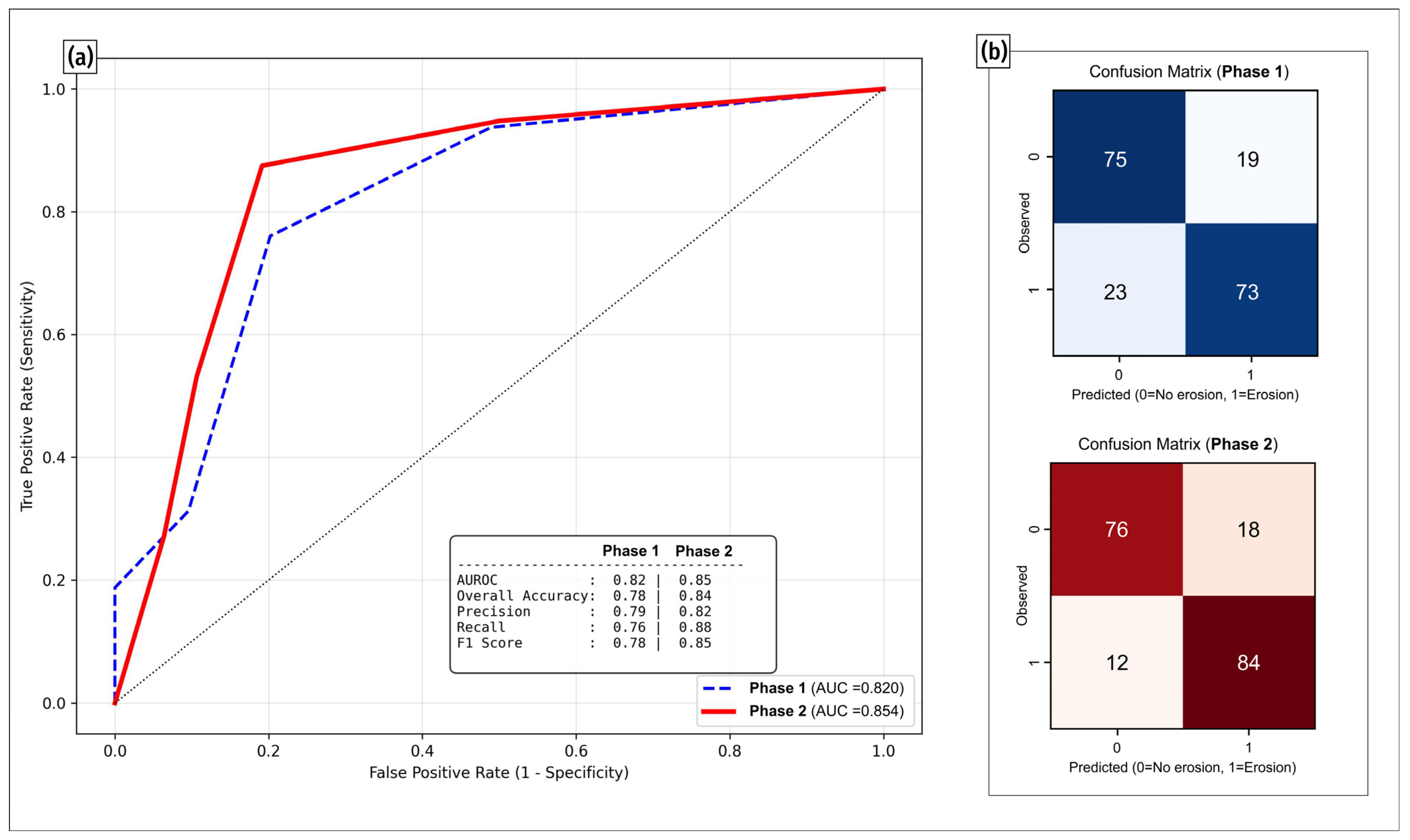
ROC analysis was applied to assess the classification capability of the Erosion Potential Model (EPM) in two phases of soil erosion assessments: Phase 1, based on desk-based modeling, and Phase 2, refined through field investigations and calibration of EPM input parameters (Figure 7a). For the purpose of ROC analysis and confusion matrix construction, binary ground truth labels (eroded/non-eroded) were assigned to each of the 190 field survey locations based on direct field observation. A location was classified as ‘eroded’ if visible erosion features (rills, gullies, mass movements, or surface wash) were documented during the field survey, and as ‘non-eroded’ if the surface was stable with no visible signs of active erosion. These field-derived binary labels served as the reference dataset against which both the desk-based (Phase 1) and field-validated (Phase 2) model predictions were evaluated. ROC curves describe the relationship between the true positive rate (TPR—sensitivity) and the false positive rate (FPR—1—specificity). This approach enables an objective evaluation of model performance independent of the selected classification threshold. The results indicate that the ROC curve for Phase 2 consistently lies above that of Phase 1, demonstrating that the EPM has improved capability to distinguish between eroded and non-eroded spatial units after field-based parameter calibration. This improvement is quantitatively confirmed by an increase in the Area Under the Curve (AUC) from 0.820 in Phase 1 to 0.854 in Phase 2, indicating a transition from a very good to a highly reliable category of classification performance. In addition to the AUC indicator, improvements in model performance in Phase 2 are supported by other statistical measures. Overall Accuracy increased from 0.78 to 0.84, while the precision increased from 0.79 to 0.82, indicating a reduction in the number of false-positive erosion classifications. At the same time, Recall increased from 0.76 to 0.88, indicating substantially improved detection of truly eroded pixels. As an integrative performance metric, the F1-score increased from 0.78 to 0.85, indicating balanced improvement in both model accuracy and sensitivity. Further insight into model performance was obtained by analyzing the confusion matrices for both phases (Figure 7b). For the desk-based soil erosion map (Phase 1), 75 non-eroded and 73 eroded spatial units were correctly identified, while 19 units were incorrectly classified as eroded, and 23 eroded units remained undetected. Confusion matrix analysis confirms the observed improvement in model performance following field validation (Phase 2), with 76 non-eroded and 84 eroded surfaces correctly classified. Overall, the results clearly indicate that including field data and calibrating input parameters significantly improve the EPM model’s discriminative ability, thereby increasing the reliability of the field-validated soil erosion map and its applicability for spatial planning and the management of erosion processes (Table S5 in the Supplementary Materials).

3.3. Analysis of the Accuracy of Soil Erosion Category Assessment

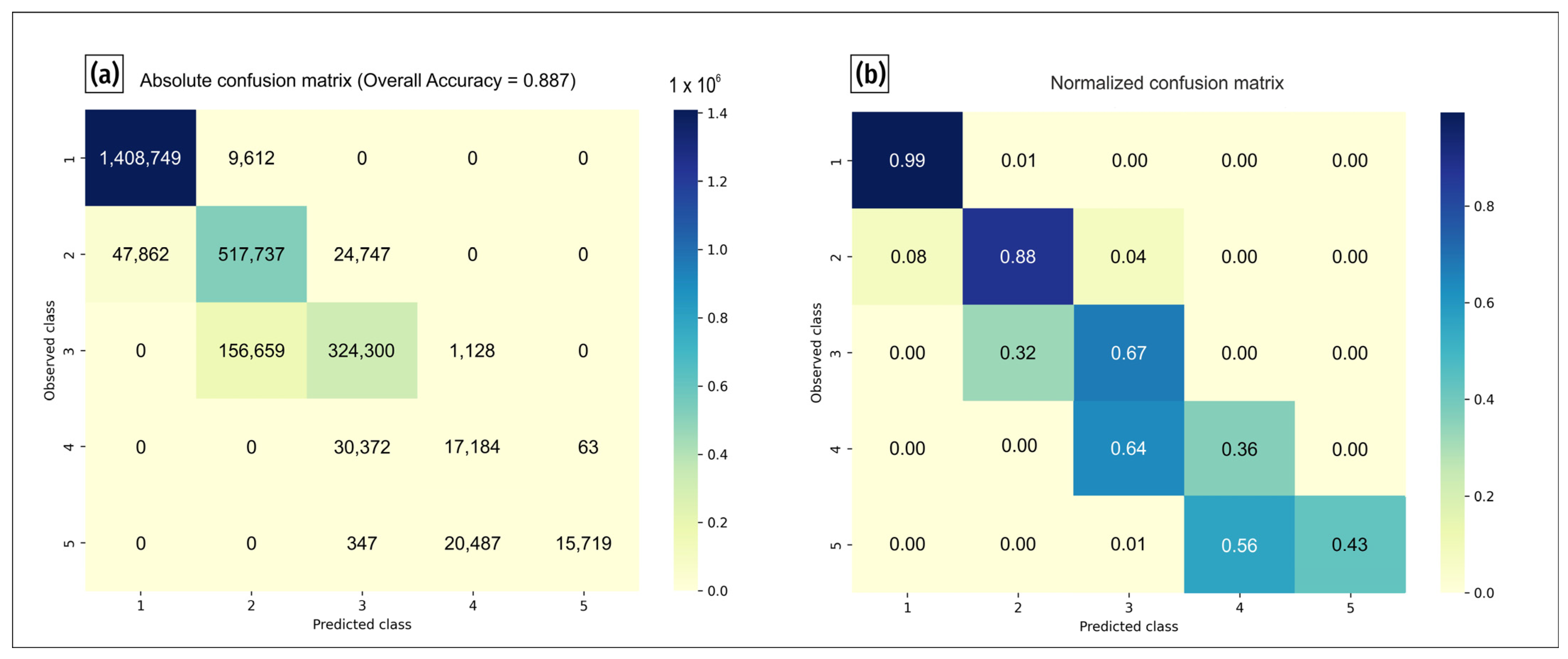
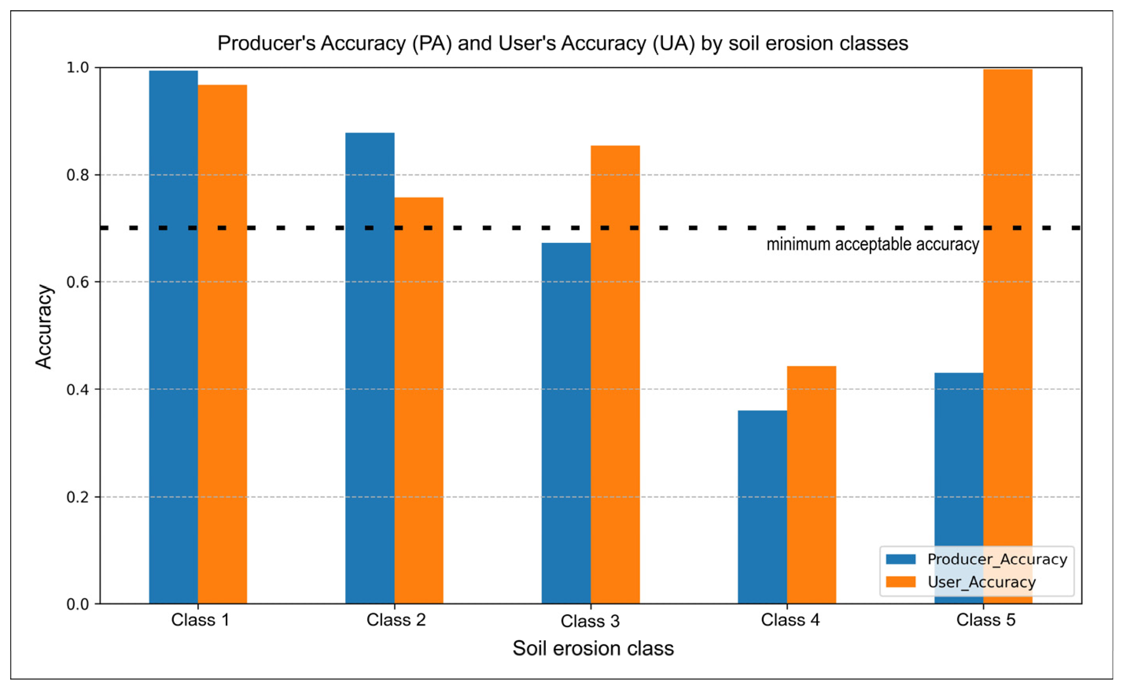
The accuracy of soil erosion model results was assessed by analyzing the absolute (Figure 8a) and normalized confusion matrices (Figure 8b) for five erosion categories (1—very slight, 2—slight, 3—medium, 4—severe, 5—excessive). The results indicate high agreement between the model predictions and the reference data, confirming the overall accuracy (Overall Accuracy = 0.88) and the Kappa coefficient (Kappa = 0.81), indicating a very good to almost complete agreement between the observed and predicted values. The absolute and normalized confusion matrices show that the highest reliability is achieved in the very slight and slight erosion classes. In contrast, the medium, severe, and excessive classes are also correctly classified to a significant extent, with the expected presence of classic errors due to their spatial heterogeneity and reduced surface representation. High values of accuracy and the Kappa coefficient confirm that the models, both in the deks-based and in the field validation phase, reliably represent the spatial distribution of erosion processes, while the field-validated map, thanks to field verification, reaches a higher level of precision. The producers’ and users’ accuracies indicate high reliability in classifying very slight erosion (class 1) in both modeling stages (Figure 9). The slight erosion class (class 2) shows a decrease in user accuracy due to overlap with the medium erosion class, while the transitional character of class 3 results in greater differences in accuracy. Lower values in the severe erosion class (class 4) reflect the spatial heterogeneity of intensive processes. The excessive erosion class (class 5) is characterized by high user but lower producer accuracy, which indicates an underestimated representation in the desk-based map. The results confirm the importance of field verification for improving classification accuracy, especially in higher erosion-intensity classes (Table S6 in the Supplementary Materials).

3.4. Analysis of the Influence of Input Factors on Erosion Processes

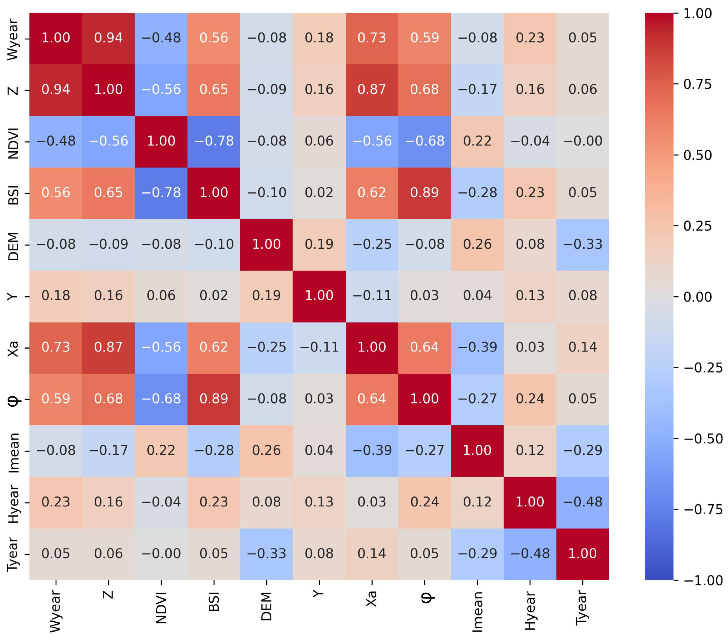
To understand the contribution of individual input factors to the formation of the intensity of erosion processes and the specific annual production of erosion material, a Pearson correlation analysis was conducted, which quantified the relationship between key morphometric, protective, and spatial parameters and the value of the erosion coefficient (Z) and the specific annual production of erosion material (W_sp) (Figure 10). The results of the Pearson correlation analysis indicate a strong dependence between the specific annual production of erosion material (W_sp) and the erosion coefficient Z (r = 0.94), confirming that the coefficient (Z) plays a key role in evaluating the intensity of erosion processes. In addition, significant positive correlations were observed with soil protection factors Xa (r = 0.73), visible erosion processes φ (r = 0.59), and the BSI (r = 0.56), indicating that degraded and poorly protected surfaces contribute dominantly to increased erosion material.

Conversely, NDVI shows a negative correlation with W_sp (r = −0.48), confirming the protective role of vegetation cover. Other factors (elevation, terrain slope, precipitation, and temperature) show reduced correlations, suggesting a less direct influence on the relationship between land cover and anthropogenic activities. The relatively low correlation between DEM (elevation) and W_sp (r = −0.08) can be explained by the indirect role of elevation in the EPM framework. Unlike slope gradient, which directly enters the erosion coefficient (Z) through the I_mean parameter, absolute elevation influences erosion processes primarily through its effect on vegetation type, land use, and climatic conditions rather than through a direct mechanistic link to erosion intensity. In the study area, higher elevations are predominantly covered by dense forest vegetation, which exerts a strong protective influence on soil surfaces. This creates an inverse relationship between elevation and erosion that partially offsets the expected positive effect of steeper slopes at higher altitudes, resulting in a near-zero net correlation. The weak correlation between annual precipitation (H_year) and W_sp (r = 0.23) reflects a fundamental characteristic of the EPM structure. In EPM, precipitation appears as a linear multiplier in the sediment production equation (Equation (1)) and does not modulate the erosion coefficient Z, which captures the spatial pattern of erosion intensity. As a result, the spatial variability of W_sp is primarily governed by Z, and by extension, by land cover, soil erodibility, visible erosion features, and slope, rather than by precipitation alone. Furthermore, the relatively modest spatial gradient of mean annual precipitation across the study area (compared to the pronounced variability in land cover and relief) limits its explanatory power in a regional correlation analysis. These findings are consistent with other regional EPM applications, where land cover and terrain variables consistently emerge as dominant drivers of erosion variability [30,35]. From the perspective of the erosion coefficient (Z), the strongest correlations were observed with Xa, BSI, φ, and NDVI, confirming that land cover condition and the intensity of surface degradation play a crucial role in shaping the area’s erosion picture. These results confirm the consistency of the EPM model and its ability to realistically depict the relationships between input factors, erosion intensity, and total erosion material production at the area level.

3.5. Spatial Distribution of Sediment Production

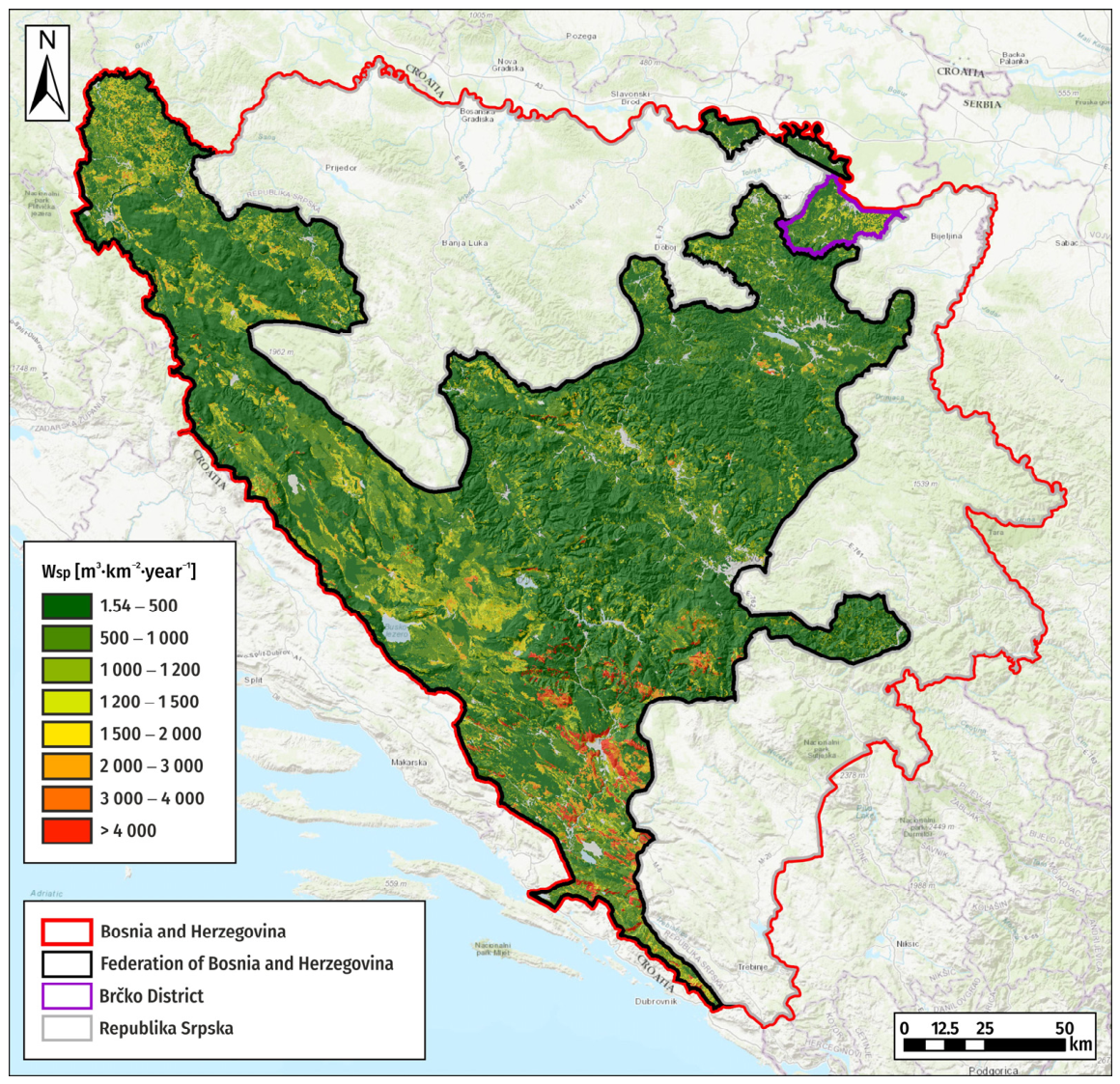
After defining the geobase of soil erosion, the erosion coefficient (Z) and key climatic parameters (average annual precipitation and temperature), the specific annual production of erosion material (W_sp) was calculated. The spatial distribution of erosion material production is shown in Figure 11, while the surface representation according to sediment production categories is shown in

Table 4. Surface representation of specific annual production of erosive material.

Category of the Sediment Production	Intensity of Erosion Processes	Dominant Erosion Type	Wsp m3∙km−2∙Year−1	km2	%
I	Excessive	Deep	>4000	332.10	1.29
I	Excessive	Surface	3000–4000	216.35	0.84
II	Severe	Deep	2000–3000	427.50	1.66
II	Severe	Surface	1500–2000	793.96	3.08
III	Medium	Deep	1200–1500	1324.61	5.14
III	Medium	Surface	1000–1200	1600.84	6.22
IV	Slight	Mixed	500–1000	5414.74	21.03
V	Very slight	Mixed	1.54–500	15,639.56	60.74
Total				25,749.66	100

. The production values reflect the strength and type of erosion processes in the researched area, which are divided according to the original EPM division [21]. The average specific annual production of erosion material for the territory of FBiH and BD is W_sp = 546.60 m³∙km⁻²∙year⁻¹, which places the area in the category of slight erosion of mixed type, with a range from 1.54 to 20,912.58 m³∙km⁻²∙year⁻¹. The total annual production of erosion material is W = 14,074,940.2 m³∙year⁻¹. The most prevalent category is very slight mixed-type erosion (60.74%), while slight mixed-type erosion accounts for 21.03% of the surface. Medium erosion-surface type includes 6.22%, and medium erosion-deep type 5.14% of the analyzed area. Severe erosion-surface type is represented at 3.08%, and severe erosion-deep type at 1.66%. Excessive surface-type erosion occupies an area of 0.84%, while excessive deep-type erosion occupies an area of 1.29%, including severe gully erosion and landslides.

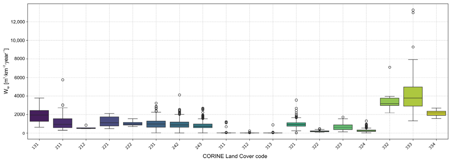
The distribution of W_sp by CORINE Land Cover (CLC) classes was analyzed (Figure 12) to examine the variability and range of values for the specific annual production of erosion material (W_sp) across land cover and land use types. The results indicate pronounced differences in erosion intensity across land cover types. The highest central values and the highest variability of W_sp were recorded in the classes that include agricultural areas with intensive cultivation, vineyards, pastures, complexes of agricultural areas, and agroforestry areas (CLC 211, 221, 231, 242, and 243), which indicates the increased sensitivity of these areas to erosion processes due to reduced soil protection and pronounced anthropogenic influence. Forest areas and thickets (CLC 311, 312, 313, 324) are characterized by significantly lower W_sp values and a narrower range of variability, which confirms the protective role of continuous vegetation cover in reducing soil erosion. Exploitation areas (CLC 131) show increased values of erosion material production with pronounced heterogeneity, which can be related to local construction activities and uneven runoff conditions. The most pronounced values and the greatest dispersion of W_sp were observed in the classes of meadows, natural grass communities, as well as in the area with scarce and sclerophyllous vegetation, bare and burnt areas (CLC 321, 323, 332, 333, 334), where extreme values also occur, which indicates a strong influence of terrain slope, vegetation cover degradation and local geomorphological conditions. Overall, the results confirm that land cover type is a key factor in the spatial variability of erosion material production, consistent with the EPM’s basic assumptions.

4. Discussion

The results of this research confirm that the EPM, when integrated with modern GIS tools and remote sensing data, represents a methodologically reliable and adaptable framework for the regional assessment of erosion processes. It is particularly significant that the application of the two-stage methodology, comprising an initial desk-based phase and a field-validated phase of field calibration of input parameters, enabled a systematic reduction in uncertainty in the spatial identification of erosion zones. The clearly expressed differences between the desk-based and field validation soil erosion maps indicate that field verification has a key role in improving the reliability of model results, especially in zones of medium and severe erosion intensity, which are usually the most sensitive to local geomorphological and pedological conditions [35,90,91].

A potential limitation of the BSI-based derivation of the φ coefficient relates to the spectral similarity between bare rock outcrops and bare or degraded soil surfaces. In karst terrain, which covers approximately 29% of the study area, limestone and dolomite rock exposures may exhibit BSI values comparable to those of eroding soil surfaces, potentially leading to an overestimation of the φ coefficient and, consequently, the erosion coefficient (Z) in rocky karst areas. To partially mitigate this issue, the EPM analysis was conducted exclusively in areas susceptible to erosion, while urban surfaces, water bodies, and wetlands were excluded from the analysis. Furthermore, the Y coefficient (soil erodibility) was assigned based on the pedological map, and areas classified as bare rock (Lithosols and rocky outcrops) received low Y values reflecting their resistance to detachment, thereby partially compensating for potential overestimation introduced through the BSI-derived φ coefficient. Nevertheless, the performance of BSI across different land cover types, particularly in distinguishing between bare rock, bare agricultural soil, and actively eroding surfaces, represents a source of residual uncertainty in this study. Future research should explore the integration of additional spectral indices or lithological masking procedures to improve the discrimination between erodible and non-erodible bare surfaces in karst-dominated landscapes.

An important methodological consideration concerns the allocation of the 190 field survey locations between parameter calibration and model validation. In this study, all field locations were used both to inform the calibration of EPM input parameters (X·a and φ) and to evaluate model performance through confusion matrix and ROC analysis. This dual use of the same dataset introduces a potential optimistic bias in the reported performance metrics, including the AUC of 0.854, as the model was assessed on data that also influenced its parameterization a form of in sample validation.

This approach was adopted due to the practical constraints of conducting field surveys across a 26,570 km² area with complex terrain and limited accessibility, where the collection of a sufficiently large independent validation dataset would have required substantially greater logistical resources. A similar approach has been employed in comparable regional-scale EPM studies [91], though its implications for model transferability should be acknowledged.

To address this limitation in future research, a stratified random partitioning of field samples (e.g., a 70/30 calibration–validation split or leave-one-out cross-validation) is recommended to provide a more conservative and independent estimate of model accuracy. The reported performance metrics should therefore be interpreted as indicative of model fit rather than strictly generalizable predictive accuracy, and the results should be considered in the context of the spatial representativeness of the sampling design across diverse geomorphological and land cover units.

A comparative analysis with existing studies that applied the EPM in the region and the wider Balkan area indicates that the average values of the erosion coefficient and the specific annual production of erosion material in this research are relatively lower compared to studies focused on smaller and more geomorphologically active watersheds [92,93]. This difference can be explained primarily by the greater spatial coverage of the analysis, which includes significant areas under stable forest and semi-natural land cover, as well as the heterogeneity of physical–geographical conditions [79,94,95,96]. Unlike local studies, which are often focused on more extreme relief conditions, the regional approach enables a more realistic assessment of the total erosion balance and the spatial distribution of the erosion potential, which avoids overestimating the intensity of erosion at the level of larger territorial entities [25,26,97]. The comparatively lower erosion coefficient values obtained in this study relative to watershed-scale EPM applications in the region can be partly attributed to differences in spatial resolution. Studies conducted at finer resolutions (10–30 m) capture steeper local slopes and smaller erosion features, thereby producing higher Z and W_sp values. At 100 m resolution, terrain gradients are smoothed through spatial averaging, which suppresses extreme slope values and reduces the computed erosion coefficient in highly dissected terrain. This scale effect is well-documented in the literature and represents an inherent trade-off between spatial resolution and the feasibility of regional-scale analysis. The 100 m resolution applied in this study is consistent with the strategic planning purpose of the outputs and with the spatial detail of the primary input dataset (CORINE Land Cover). However, this resolution prevents the detection of linear erosion features such as rills and gullies, which may be significant contributors to total sediment yield in specific sub-catchments. This limitation is acknowledged and should be considered when interpreting the results at sub-regional or local scales.

The results of this research are consistent with recent global estimates of soil erosion based on EPM and its modified versions, which, for the observed area, also indicate the dominance of slight erosion [16]. Observed deviations in the absolute values of the erosion coefficient (Z) and production of eroded material (W_sp) can be interpreted as an expected consequence of differences in spatial resolution, quality, and sources of input data, as well as the application of regionally adjusted parameters and field verification. These findings indicate that global and regional EPM approaches are not competitive but complementary: while global models provide a consistent framework for interregional comparisons and the identification of general patterns of erosion potential, regionally calibrated analyses allow greater sensitivity to local geomorphological, pedological, and anthropogenic factors.

The reduced classification accuracy observed for the medium and severe erosion classes warrants a more detailed examination of potential sources of discrepancy, including the temporal alignment between spectral data acquisition and field surveys. In this study, the NDVI and BSI indices were computed as multi-temporal composites derived from Landsat imagery spanning the period from January 2010 to December 2020, while field surveys were conducted between June and December 2021. Although the use of a ten-year composite is intended to capture the stable, long-term characteristics of vegetation cover and bare soil exposure, thereby minimising the influence of short-term seasonal fluctuations a degree of temporal mismatch between the spectral signal and the field-observed conditions is unavoidable.

This temporal offset is particularly relevant for the medium erosion class, which is characterised by transitional land cover types (e.g., transitional woodland–shrub, degraded pastures, and areas under shifting agricultural use) that exhibit pronounced seasonal and inter-annual variability in vegetation density. In such environments, NDVI values computed from a decadal composite may not accurately reflect the vegetation cover conditions encountered during field surveys, potentially leading to discrepancies in the assignment of X·a coefficient values and, consequently, in the classification of erosion intensity.

For the severe and excessive erosion classes, the reduced producer’s accuracy suggests that some actively eroding surfaces characterised by dynamic and episodic processes such as gully incision, mass movements, and rill development may not be consistently detectable through multi-temporal spectral composites, particularly if the erosion events occurred after the end of the Landsat time series (post-2020). Future studies should consider using shorter temporal windows for spectral index computation, ideally aligned with the field survey period, and should explore the use of more recent and higher-temporal-resolution imagery (e.g., Sentinel-2) to improve the temporal consistency between remote sensing inputs and field observations.

Analysis of erosion material production by land use type confirms the central role of land cover as a key regulator of erosion processes [98,99,100]. The increased values of the production of eroded material on agricultural and degraded grass surfaces are in accordance with the theoretical assumptions of the EPM and numerous empirical studies that indicate the negative effect of intensive soil cultivation and fragmented vegetation cover [30,101,102,103,104,105]. In contrast, stable forest ecosystems show a distinctly protective function in surface runoff control and soil stabilization, thus confirming their importance in the preservation of land and water resources at the regional level.

The identification of 1319.12 km² of territory affected by medium-to-excessive erosion, representing areas requiring priority soil conservation intervention, carries direct implications for environmental policy and spatial planning in the Federation of Bosnia and Herzegovina and Brčko District.

At the strategic level, the field-validated soil erosion map provides a spatially explicit basis for prioritizing erosion control investments within the framework of national and entity-level water management plans, including the Strategy for Water Management of the Federation of Bosnia and Herzegovina. Priority intervention zones, particularly those classified as severe or excessive erosion, should be integrated into cantonal and municipal spatial plans as areas requiring binding land use restrictions and targeted anti-erosion measures.

At the operational level, the identified hotspots, which are concentrated in areas of degraded pasture, fragmented agricultural land, and transitional woodland–shrub zones, call for specific conservation measures, including the establishment of permanent vegetation cover, reforestation of degraded slopes, construction of check dams and retention structures in active torrent channels, and restrictions on land conversion from forest to agricultural use [106]. The overlay of erosion priority zones with the existing torrent stream network could further support the identification of catchments at elevated risk of torrential flooding, thereby linking soil conservation planning with disaster risk reduction.

Given the severe human and material losses caused by the 2014 and 2024 torrential flood events in BiH, the timely integration of these results into national resilience frameworks, including the Sendai Framework for Disaster Risk Reduction, represents both a scientific imperative and a societal responsibility.

5. Advantages and Limitations

The primary advantage of this study lies in the application of a combined desk-based and field-based approach, through which the EPM was adapted to the regional conditions of the FBiH and BD. The integration of the analytical EPM model, a GIS environment, remote sensing data, and field verification reduced uncertainty in the estimation of the erosion coefficient (Z) and enabled a more realistic assessment of erosion material production (W and W_sp) compared to exclusively desk-based or global approaches. A particular strength of the study is reflected in the possibility of directly comparing regionally calibrated results with contemporary global EPM estimates, thereby confirming both the methodological consistency of the applied approach and the importance of local calibration of input parameters [21,22,35].

A fundamental constraint of the proposed methodology relates to the 100 m spatial resolution adopted for all analytical layers. While this resolution is consistent with the spatial detail of the CORINE Land Cover dataset and appropriate for strategic regional-scale planning, it inherently limits the detection of sub-pixel erosion processes that are particularly significant in complex mountainous environments. Specifically, linear erosion features such as rills, ephemeral gullies, and small torrential channels typically range from decimetres to a few metres in width, rendering them effectively invisible at 100 m resolution. Similarly, localised mass movement scarps, shallow landslide initiation zones, and small erosion patches within otherwise stable landscape units may be systematically underrepresented or averaged out during spatial aggregation.

This resolution-induced smoothing has two principal consequences for the results. First, the mean slope coefficient (I_mean), derived from the resampled DEM, underestimates local gradient extremes in highly dissected terrain, leading to a potential underestimation of the erosion coefficient Z in areas with pronounced micro-relief. Second, spectral indices (NDVI and BSI) computed at 100 m integrate the radiometric signal from multiple land cover types within a single pixel, which may mask the presence of small bare or eroding patches within otherwise vegetated or forested areas. The resulting mixed-pixel effect could lead to an overestimation of vegetation protection (X·a) and an underestimation of visible erosion intensity (φ) in heterogeneous landscape units.

These limitations are acknowledged as inherent trade-offs of the regional-scale approach and should be considered when interpreting the outputs at sub-regional or local scales. Future research should prioritise higher-resolution analyses employing UAV-based photogrammetry, LiDAR data, or Sentinel-2 imagery at 10 m resolution particularly for cantonal and municipal-scale erosion assessments and for the detailed characterisation of erosion hotspots identified in this study.

A further limitation concerns the extent of field investigations, conducted at 190 locations over an area of approximately 26,570 km². Although this number of samples is consistent with recommendations for regional studies and enables statistically robust model validation, a higher sampling density would be required for local-scale analyses in areas characterized by pronounced geomorphological heterogeneity [107]. From a methodological perspective, an additional limitation of the EPM arises from its deterministic and semi-empirical nature, which does not fully capture the nonlinear interactions among climatic, pedological, and anthropogenic factors [98,99].

Future research should integrate EPM with machine learning [108,109], and climate change scenarios [110] and land-cover change simulations [111,112,113,114,115]. Such an approach would enable a transition from static to prognostic analyses, which are essential for the long-term planning of soil-conservation measures and the management of torrential flood risk [116].

Despite the aforementioned limitations, the results of this study confirm that a regionally calibrated soil erosion map represents an important link between global assessments and operational spatial management, with significant applicability in spatial planning, the definition of priority zones, and the implementation of soil-conservation measures at the regional level.

6. Conclusions

This study confirms that integrating the EPM with GIS tools, satellite data, and systematic field verification provides a reliable framework for regional-scale soil erosion mapping. By combining desk-based modelling with field calibration, the spatial accuracy and reliability of the field-validated soil erosion map for the FBiH and BD were significantly improved. The incorporation of spectral indices NDVI and BSI, derived from Landsat satellite imagery, enabled a more objective assessment of vegetation cover conditions and visible erosion features, thereby further enhancing the parameterization of the EPM model. Model validation using ROC/AUC analysis and a confusion matrix indicated high discriminatory performance and clearly confirmed the importance of field calibration, particularly in areas characterized by moderate to high erosion intensity. The results revealed pronounced spatial heterogeneity in erosion processes, with degraded and poorly protected areas identified as the dominant sources of erosion material.

The field-validated soil erosion map provides a reliable spatial basis for identifying priority degradation zones, planning soil and water conservation measures, and reducing torrential flood risk at the regional level. Beyond its immediate applicability, the proposed methodological framework establishes a functional link between global erosion assessments and regionally adapted tools for operational spatial management. Future research should focus on integrating satellite data with higher spatial and temporal resolution, incorporating climate change scenarios, and developing hybrid approaches combining the EPM with machine learning methods. Such an approach could further enhance predictive accuracy and enable dynamic monitoring of erosion processes under conditions of accelerated climatic and anthropogenic change.

References

1. Gianinetto, M.; Aiello, M.; Vezzoli, R.; Polinelli, F.N.; Rulli, M.C.; Chiarelli, D.D.; Bocchiola, D.; Ravazzani, G.; Soncini, A. Future Scenarios of Soil Erosion in the Alps under Climate Change and Land Cover Transformations Simulated with Automatic Machine Learning. Climate 2020, 8, 28. [Google Scholar] [CrossRef] [Scilit]
2. Oldeman, L.R.; Hakkeling, R.T.A.; Sombroek, W.G. World Map on the Status of Human Induced Soil Degradation, with Explanatory Note (Second Revised Edition); UNEP: Athens, Greece, 1991. [Google Scholar]
3. Gobin, A.; Jones, R.; Kirkby, M.; Campling, P.; Govers, G.; Kosmas, C.; Gentile, A.R. Indicators for Pan-European Assessment and Monitoring of Soil Erosion by Water. Environ. Sci. Policy 2004, 7, 25–38. [Google Scholar] [CrossRef] [Scilit]
4. van der Knijff, J.M.; Jones, R.J.A.; Montanarella, L. Soil Erosion Risk Assessment in Europe; EUR 19022; Office for Official Publications of the European Communities: Luxembourg, 2000. [Google Scholar]
5. Panagos, P.; Borrelli, P.; Poesen, J.; Ballabio, C.; Lugato, E.; Meusburger, K.; Montanarella, L.; Alewell, C. The New Assessment of Soil Loss by Water Erosion in Europe. Environ. Sci. Policy 2015, 54, 438–447. [Google Scholar] [CrossRef] [Scilit]
6. Panagos, P.; Standardi, G.; Borrelli, P.; Lugato, E.; Montanarella, L.; Bosello, F. Cost of Agricultural Productivity Loss Due to Soil Erosion in the European Union: From Direct Cost Evaluation Approaches to the Use of Macroeconomic Models. Land Degrad. Dev. 2018, 29, 471–484. [Google Scholar] [CrossRef] [Scilit]
7. Borrelli, P.; Panagos, P.; Montanarella, L. New Insights into the Geography and Modelling of Wind Erosion in the European Agricultural Land. Application of a Spatially Explicit Indicator of Land Susceptibility to Wind Erosion. Sustainability 2015, 7, 8823–8836. [Google Scholar] [CrossRef] [Scilit]
8. McIvor, I.; Youjun, H.; Daoping, L.; Eyles, G.; Pu, Z. Agroforestry: Conservation Trees and Erosion Prevention. In Encyclopedia of Agriculture and Food Systems; Elsevier: Amsterdam, The Netherlands, 2014; pp. 208–221. [Google Scholar]
9. Jarrah, M.; Mayel, S.; Tatarko, J.; Funk, R.; Kuka, K. A Review of Wind Erosion Models: Data Requirements, Processes, and Validity. CATENA 2020, 187, 104388. [Google Scholar] [CrossRef] [Scilit]
10. Nordstrom, K.F.; Hotta, S. Wind Erosion from Cropland in the USA: A Review of Problems, Solutions and Prospects. Geoderma 2004, 121, 157–167. [Google Scholar] [CrossRef] [Scilit]
11. Iturri, L.A.; Buschiazzo, D.E. Interactions between Wind Erosion and Soil Organic Carbon. In Agricultural Soil Sustainability and Carbon Management; Elsevier: Amsterdam, The Netherlands, 2023; pp. 163–179. [Google Scholar]
12. Ristić, R.; Kostadinov, S.; Abolmasov, B.; Dragićević, S.; Trivan, G.; Radić, B.; Trifunović, M.; Radosavljević, Z. Torrential Floods and Town and Country Planning in Serbia. Nat. Hazards Earth Syst. Sci. 2012, 12, 23–35. [Google Scholar] [CrossRef] [Scilit]
13. Prăvălie, R.; Borrelli, P.; Panagos, P.; Ballabio, C.; Lugato, E.; Chappell, A.; Miguez-Macho, G.; Maggi, F.; Peng, J.; Niculiță, M.; et al. A Unifying Modelling of Multiple Land Degradation Pathways in Europe. Nat. Commun. 2024, 15, 3862. [Google Scholar] [CrossRef] [Scilit] [PubMed]
14. Afshar, M.H.; Hassani, A.; Aminzadeh, M.; Borrelli, P.; Panagos, P.; Robinson, D.A.; Or, D.; Shokri, N. Spatial and Temporal Assessment of Soil Degradation Risk in Europe. Sci. Rep. 2025, 15, 44636. [Google Scholar] [CrossRef] [Scilit]
15. Zoka, M.; Lladó, S.; Stathopoulos, N.; Kokkalidou, M.; Ventura, A.M.; Stringer, L.C.; Baarsma, B.; Trakal, L.; Gorfer, M.; Codina, S. Preliminary Assessment of the Knowledge Gaps to Reduce Land Degradation in Europe. Soils Eur. 2024, 1, e119137. [Google Scholar] [CrossRef] [Scilit]
16. Bezak, N.; Borrelli, P.; Mikoš, M.; Jemec Auflič, M.; Panagos, P. Towards Multi-Model Soil Erosion Modelling: An Evaluation of the Erosion Potential Method (EPM) for Global Soil Erosion Assessments. CATENA 2024, 234, 107596. [Google Scholar] [CrossRef] [Scilit]
17. Brandolini, F.; Kinnaird, T.C.; Srivastava, A.; Turner, S. Modelling the Impact of Historic Landscape Change on Soil Erosion and Degradation. Sci. Rep. 2023, 13, 4949. [Google Scholar] [CrossRef] [Scilit]
18. Abeje, A.; Tsegaye, D.; Bayu, T.Y. Geospatial Assessment of Erosion Intensity and Prioritization of Vulnerable Areas in the Shafe Catchment, South Ethiopian Rift Valley. Discov. Sustain. 2025, 6, 911. [Google Scholar] [CrossRef] [Scilit]
19. Sestras, P.; Mircea, S.; Roșca, S.; Ștefan, B.; Sălăgean, T.; Dragomir, L.O.; Herbei, M.V.; Bruma, S.; Sabou, C.; Marković, R.; et al. GIS Based Soil Erosion Assessment Using the USLE Model for Efficient Land Management: A Case Study in an Area with Diverse Pedogeomorphological and Bioclimatic Characteristics. Not. Bot. Horti Agrobot. Cluj-Napoca 2023, 51, 13263. [Google Scholar] [CrossRef] [Scilit]
20. Yao, E. Coupling Benefit of Land Use, Land Cover Change and Soil Erosion Under Algorithmic Optimization Model. ICST Trans. Scalable Inf. Syst. 2024, 12, 1. [Google Scholar] [CrossRef] [Scilit]
21. Gavrilović, S. Engineering of Torrents and Erosion; Journal of Construction (Special Issue): Belgrade, Yugoslavia, 1972. (In Serbian) [Google Scholar]
22. Gavrilović, S. A Method for Estimating the Average Annual Quantity of Sediments According to the Potency of Erosion. Bull. Fac. For.-Belgrade 1962, 26, 151–168. [Google Scholar]
23. Vučićević, D. Uređenje Bujičnih Tokova-Priručnik Za Bujičare; Društvo bujičara Jugoslavije: Belgrade, Yugoslavia, 1995. (In Serbian) [Google Scholar]
24. Kostadinov, S. Bujični Tokovi i Erozija; Univerzitet u Beogradu, Šumarski Fakultet: Belgrade, Serbia, 2008. (In Serbian) [Google Scholar]
25. Malušević, I.; Ristić, R.; Radić, B.; Polovina, S.; Milčanović, V.; Nešković, P. A Historical Overview of Methods for the Estimation of Erosion Processes on the Territory of the Republic of Serbia. Land 2025, 14, 405. [Google Scholar] [CrossRef] [Scilit]
26. Stefanidis, S.P.; Proutsos, N.D.; Tigkas, D.; Chatzichristaki, C. Erosion-Based Classification of Mountainous Watersheds in Greece: A Geospatial Approach. Sustainability 2025, 17, 8710. [Google Scholar] [CrossRef] [Scilit]
27. Lazarević, R. Erozija u Bosni i Hercegovini; Želnid: Belgrade, Serbia, 2010. (In Serbian) [Google Scholar]
28. Trendafilov, B.; Minchev, I.; Trendafilov, A.; Blinkov, I. Comparison of EPM with Rusle for Soil Erosion Modeling in the Strumica River Basin. Geogr. Environ. Sustain. 2025, 17, 44–49. [Google Scholar] [CrossRef] [Scilit]
29. Blinkov, I. Review and Comparison of Water Erosion Intensity in the Western Balkan and EU Countries. Contrib. Sect. Nat. Math. Biotech. Sci. MASA 2015, 1, 27–42. [Google Scholar] [CrossRef] [Scilit]
30. Spalevic, V.; Barovic, G.; Vujacic, D.; Curovic, M.; Behzadfar, M.; Djurovic, N.; Dudic, B.; Billi, P. The Impact of Land Use Changes on Soil Erosion in the River Basin of Miocki Potok, Montenegro. Water 2020, 12, 2973. [Google Scholar] [CrossRef] [Scilit]
31. Petras, J.; Kuspilic, N.K.D. Some Experience on the Prediction of Suspended Sediment Concentrations and Fluxes in Croatia. In Proceedings of the Symposium SI Held During the Seventh IAHS Scientific Assembly at Foz do Igacu, Brazil; IAHS: Wallingford, UK, 2005; Volume 292, pp. 179–184. [Google Scholar]
32. Dragičević, N.; Karleuša, B.; Ožanić, N. Modification of erosion potential method using climate and land cover parameters. Geomat. Nat. Hazards Risk 2018, 9, 1085–1105. [Google Scholar] [CrossRef] [Scilit]
33. Zemljic, M. Calculation of Sediment Load. Evaluation of Vegetation as Anti-Erosive Factor. In Proceedings of the International Symposium Interpraevent, Villach (Australia); INTERPRAEVENT: Vienna, Austria, 1971. [Google Scholar]
34. Globevnik, L.; Holjević, D.; Petkovšek, G.; Rubinić, J. Applicability of the Gavrillović Method in Erosion Calculation Using Spatial Data Manipulation Techniques; IAHS-AISH Publication: Reykjavik, Iceland, 2003; pp. 224–233. [Google Scholar]
35. Zorn, M.; Komac, B. Response of Soil Erosion to Land Use Change with Particular Reference to the Last 200 Years (Julian Alps, Western Slovenia). Rev. Geomorfol. 2009, 11, 39–47. [Google Scholar]
36. De Cesare, G.; Beyer Portner, N.; Boillat, J.S.A. Modelling of Erosion and Sedimentation Based on Field Investigation in Alpine Reservoirs of Hydropower Schemes. In Proceedings of the German Coastal Engineering Research Council, Parallel Session 34; American Society of Civil Engineers: Reston, VA, USA, 1998. [Google Scholar]
37. de Vente, J.; Poesen, J.; Bazzoffi, P.; Van Rompaey, A.; Verstraeten, G. Predicting Catchment Sediment Yield in Mediterranean Environments: The Importance of Sediment Sources and Connectivity in Italian Drainage Basins. Earth Surf. Process. Landforms 2006, 31, 1017–1034. [Google Scholar] [CrossRef] [Scilit]
38. Fanetti, D.; Vezzoli, L. Sediment Input and Evolution of Lacustrine Deltas: The Breggia and Greggio Rivers Case Study (Lake Como, Italy). Quat. Int. 2007, 173–174, 113–124. [Google Scholar] [CrossRef] [Scilit]
39. Milanesi, L.; Pilotti, M.; Clerici, A. The Application of the Erosion Potential Method to Alpine Areas: Methodological Improvements and Test Case. In Engineering Geology for Society and Territory; Springer: Cham, Switzerland, 2015; Volume 3, pp. 347–350. [Google Scholar] [CrossRef] [Scilit]
40. Emmanouloudis, D.A.; Christou, O.P.; Filippidis, E.I. Quantitative Estimation of Degradation in the Aliakmon River Basin Using GIS. In Proceedings of Symposium HS01 Held During IUGG2003 at Sapporo, July 2003; IAHS-AISH Publication: Wallingford, CT, USA, 2003; pp. 234–240. [Google Scholar]
41. Kalinderis, I.; Tziaftani, F.; Sapountzis, M.; Kourakli, P.; Stefanidis, P.; Stathis, D. The Risk of Sedimentation of Artificial Lakes, Following the Soil Loss and Degradation Process in the Wider Drainage Basin. Artificial Lake of Smokovo Case Study (Central Greece). In Proceedings of the Global Change and Soil Management: From Degradation Through Soil and Water Conservation to Sustainable Soil Management; Catena-Verl: Reiskirchen, Germany, 2009. [Google Scholar]
42. Ahmed, A.; Adil, D.; Hasna, B.; Elbachir, A.; Lazaar, R. Using EPM Model and GIS for Estimation of Soil Erosion in Souss Basin, Morocco. Turkish J. Agric.-Food Sci. Technol. 2019, 7, 1228–1232. [Google Scholar] [CrossRef] [Scilit]
43. da Silva, R.M.; Santos, C.A.G.; Silva, A.M. Predicting Soil Erosion and Sediment Yield in the Tapacurá Catchment. J. Urban Environ. Eng. 2014, 8, 75–82. [Google Scholar] [CrossRef] [Scilit]
44. Lense, G.H.E.; Parreiras, T.C.; Moreira, R.S.; Avanzi, J.C.; Mincato, R.L. Estimates of Soil Losses by the Erosion Potential Method in Tropical Latosols. Cienc. Agrotec. 2019, 43, e012719. [Google Scholar] [CrossRef] [Scilit]
45. Rafaelli, S.; Peviani, M.; Ayala, F.P. Study of Sediment Yield on the Mountain Cuence Del Rio Iruya (Argentina). In Proceedings of the IARH AMH, Hydraulic XVIII Latin American Conference, Oaxaca, Mexico, 13–16 October 1998. [Google Scholar]
46. de Vente, J.; Poesen, J. Predicting Soil Erosion and Sediment Yield at the Basin Scale: Scale Issues and Semi-Quantitative Models. Earth-Sci. Rev. 2005, 71, 95–125. [Google Scholar] [CrossRef] [Scilit]
47. Ali, S.S.; Al-Umary, F.A.; Salar, S.G.; Al-Ansari, N.; Knutsson, S. GIS Based Soil Erosion Estimation Using EPM Method, Garmiyan Area, Kurdistan Region, Iraq. J. Civ. Eng. Archit. 2016, 10, 291–308. [Google Scholar] [CrossRef] [Scilit]
48. Amini, H.; Honarjoo, N.; Jalaliyan, A.; Khalilizadeh, M.B.J. A Comparison of EPM and WEPP Models for Estimating Soil Erosion of Marmeh Watershed in the South Iran. Agric. For. 2014, 60, 299–315. [Google Scholar]
49. Kazimierski, L.D.; Irigoyen, M.; Re, M.; Menendez, A.N.; Spalletti, P.; Brea, J.D. Impact of Climate Change on Sediment Yield from the Upper Plata Basin. Int. J. River Basin Manag. 2013, 11, 411–421. [Google Scholar] [CrossRef] [Scilit]
50. Otoniel, N.P. Identificación de Correlaciones Entre La Arga de Lavado y Algunos Parámetros Geomorfológicos y de Uso de Suelo En La Cuenca Del Río Cauca. Master’s Thesis, Universidad Nacional de Colombia, Bogotá, Colombia, 2015. [Google Scholar]
51. Renard, K.; Foster, G.; Weesies, G.; McCool, D.; Yoder, D. Predicting Soil Erosion by Water: A Guide to Conservation Planning with the Revised Universal Soil Loss Equation (RUSLE); Agric. Handb. No. 703; United States Government Printing: Washington, DC, USA, 1997; p. 703. ISBN 0-16-048938-5.
52. Federalno Ministarstvo Poljoprivrede Vodoprivrede i Šumarstva. Strategija Upravljanja Vodama Federacije Bosne i Hercegovine 2010–2022. 2012; 300p. Available online: https://faolex.fao.org/docs/pdf/bih204311.pdf (accessed on 3 April 2026).
53. Federalna Uprava Civilne Zaštite Procjena Ugroženosti Federacije Bosne i Hercegovine Od Prirodnih i Drugih Nesreća. Available online: https://fucz.gov.ba/procjena-ugrozenosti-f-bih-od-prirodnih-i-drugih-nesreca/ (accessed on 3 April 2026).
54. Izvještaj o Realizaciji Sredstava Za Sanaciju Posljedica Poplava u BIH Iz 2014. Godine, Sarajevo, Mart 2016. Available online: https://www.cpi.ba/wp-content/uploads/2020/04/FINALNI-IZVJE%C5%A0TAJ-O-REALIZACIJI-SREDSTAVA-ZA-SANACIJU-POSLJEDICA-POPLAVA-U-BIH-IZ-2014.-GODINE.pdf (accessed on 3 April 2026).
55. GFDRR-Global Facility for Disaster Reduction and Recovery. Bosnia and Herzegovina Floods 2014 Recover Needs Assessment. Available online: https://www.gfdrr.org/en/publication/bosnia-and-herzegovina-floods-2014-recover-needs-assessment (accessed on 3 April 2026).
56. European Union; United Nations; World Bank. Bosnia and Herzegovina Recovery Needs Assessment; European Union-United Nations: Brussels, Belgium, 2014. [Google Scholar]
57. UN. Bosnia and Herzegovina Floods Response—Multi-Cluster Initial Rapid Assessment; United Nations in Bosnia and Herzegovina: Sarajevo, Bosnia and Herzegovina, 2024; pp. 1–21. [Google Scholar]
58. IFRC. DREF Final Report. Available online: https://reliefweb.int/report/bosnia-and-herzegovina/bosnia-and-herzegovina-pluvialflash-flood-2024-dref-final-report-mdrba017 (accessed on 13 February 2026).
59. Kirby, P.; Delauney, G. Delauney Bosnia: Floods and Landslides Leave 18 Dead. Available online: https://www.bbc.com/news/articles/c4g5elll48lo (accessed on 13 February 2026).
60. Vulovic, M. The Impact of Floods and Landslides on the 2024 Local Elections in Bosnia and Herzegovina; International Institute for Democracy and Electoral Assistance (International IDEA): Stockholm, Sweden, 2025. [Google Scholar]
61. Ristić, R.; Solomun, M.K.; Malušević, I.; Ždrale, S.; Radić, B.; Polovina, S.; Milćanović, V. Healthy Soils—Healthy People: Soil and Human Health—The Reality of the Balkan Region. In The Soil-Human Health-Nexus; CRC Press: Boca Raton, FL, USA, 2020; pp. 223–248. [Google Scholar] [CrossRef] [Scilit]
62. (UNEP) United Nations Environmental Programme. Sarajevo Action Program for Combat Land Degradation and Mitigate the Effects of Drought in Bosnia and Herzegovina; GEF: Bosnia and Herzegovina, Sarajevo, 2017. [Google Scholar]
63. Federalni Zavod Za Agropedologiju. Osnovna Pedološka Karta Bosne i Hercegovine 1:50,000. Available online: https://agropedologija.gov.ba/pedoloska-karta-bosne-i-hercegovine/ (accessed on 3 April 2026).
64. CORINE Land Cover—Copernicus Land Monitoring Service. Available online: https://land.copernicus.eu/en/products/corine-land-cover (accessed on 19 March 2024).
65. Law, M.; Collins, A. Getting to Know ArcGIS Desktop 10.8; Esri Press: Redlands, CA, USA, 2021. [Google Scholar]
66. (GEE) Google Earth Engine. Data Catalog. Available online: https://developers.google.com/earth-engine/datasets/catalog/landsat (accessed on 24 May 2024).
67. Federalni Hidrometeorološki Zavod Klimatski Podaci—Srednja Godišnja Temperatura i Količine Padavina Za Federaciju BiH. Available online: https://www.fhmzbih.gov.ba/latinica/METEO/prognozaBI.php (accessed on 13 February 2026).
68. UNFCCC (United Nations Framework Convention on Climate Change—Bosna i Hercegovina). Klimatske Karakteristike Bosne i Hercegovine. Available online: https://www.unfccc.ba/lat/analize-lat/klimatskekarakteristikebih-lat (accessed on 13 February 2026).
69. Republički Hidrometeorološki Zavod Republike Srpske Klimatski Podaci—Srednja Godišnja Temperatura i Količine Padavina Za Republiku Srpsku. Available online: https://rhmzrs.com/page/meteorologija-godisnji-pregled (accessed on 13 February 2026).
70. Copernicus Land Monitoring Service. EU-DEM v1.1—Digital Elevation Model of Europe (25 m); European Environment Agency: Copenhagen, Denmark, 2020.
71. U.S. Geological Survey. EarthExplorer—Gateway to Earth Observation Data. Available online: https://earthexplorer.usgs.gov (accessed on 12 February 2026).
72. Johnston, K.; Hoef, V.J.M.; Krivoruchko, K.; Lucas, N. Using ArcGIS Geostatistical Analyst, Environmental Systems Research; Environmental Systems Research: Redlands, CA, USA, 2001. [Google Scholar]
73. Levin, N. Fundamentals of Remote Sensing; Remote Sensing Laboratory, Geography Department, Tel Aviv University: Tel Aviv, Israel, 1999. [Google Scholar]
74. Khorram, S.; van der Wiele, C.F.; Koch, F.H.; Nelson, S.A.C.; Potts, M.D. Principles of Applied Remote Sensing; Springer International Publishing: Cham, Switzerland, 2016. [Google Scholar]
75. Deering, D.W. Rangeland Reflectance Characteristics Measured by Aircraft and Spacecraft Sensors. Ph.D. Thesis, Texas A&M University, Libraries, College Station, TX, USA, 1978. [Google Scholar]
76. Rikimaru, A.; Roy, P.; Miyatake, S. Tropical Forest Cover Density Mapping. Trop. Ecol. 2002, 43, 39–47. [Google Scholar]
77. Polovina, S.; Radić, B.; Ristić, R.; Milčanović, V. Application of Remote Sensing for Identifying Soil Erosion Processes on a Regional Scale: An Innovative Approach to Enhance the Erosion Potential Model. Remote Sens. 2024, 16, 2390. [Google Scholar] [CrossRef] [Scilit]
78. Diek, S.; Fornallaz, F.; Schaepman, M.E.; De Jong, R. Barest Pixel Composite for Agricultural Areas Using Landsat Time Series. Remote Sens. 2017, 9, 1245. [Google Scholar] [CrossRef] [Scilit]
79. Petrović, A.M.; Guerit, L.; Nikolova, V.; Novković, I.; Filipov, D.; Jakubínský, J. Quantifying Torrential Watershed Behavior over Time: A Synergistic Approach Using Classical and Modern Techniques. Earth 2025, 7, 1. [Google Scholar] [CrossRef] [Scilit]
80. Imširović, Š.; Polovina, S.; Hadžialić, A.; Radić, B.; Ristić, R.; Milčanović, V. Spatial Identification of Erosion Processes in the Sarajevo Canton. Erozija 2025, 51, 7–30. [Google Scholar] [CrossRef] [Scilit]
81. Milanović, S.; Milanović, S.D.; Marković, N.; Pamučar, D.; Gigović, L.; Kostić, P. Forest Fire Probability Mapping in Eastern Serbia: Logistic Regression versus Random Forest Method. Forests 2021, 12, 5. [Google Scholar] [CrossRef] [Scilit]
82. Fawcett, T. An Introduction to ROC Analysis. Pattern Recognit. Lett. 2006, 27, 861–874. [Google Scholar] [CrossRef] [Scilit]
83. Joshi, B.R.; Bhandary, N.P.; Acharya, I.P.; KC, N.; Bhandari, C. Landslide Susceptibility Mapping Optimization for Improved Risk Assessment Using Multicollinearity Analysis and Machine Learning Technique. Appl. Sci. 2025, 15, 12152. [Google Scholar] [CrossRef] [Scilit]
84. Cohen, J. A Coefficient of Agreement for Nominal Scales. Educ. Psychol. Meas. 1960, 20, 37–46. [Google Scholar] [CrossRef] [Scilit]
85. Landis, J.R.; Koch, G.G. The Measurement of Observer Agreement for Categorical Data. Biometrics 1977, 33, 159. [Google Scholar] [CrossRef] [Scilit]
86. Tempfli, K.; Huurneman, G.C.; Bakker, W.H.; Janssen, L.L.F.; Feringa, W.F.; Gieske, A.S.M.; Grabmaier, K.A.; Hecker, C.A.; Horn, J.A.; Kerle, N.; et al. Principles of Remote Sensing: An Introductory Textbook; International Institute for Geo-Information Science and Earth Observation: Enschede, The Netherlands, 2009. [Google Scholar]
87. Olofsson, P.; Foody, G.M.; Herold, M.; Stehman, S.V.; Woodcock, C.E.; Wulder, M.A. Good Practices for Estimating Area and Assessing Accuracy of Land Change. Remote Sens. Environ. 2014, 148, 42–57. [Google Scholar] [CrossRef] [Scilit]
88. Maxwell, A.E.; Warner, T.A.; Guillén, L.A. Accuracy Assessment in Convolutional Neural Network-Based Deep Learning Remote Sensing Studies—Part 1: Literature Review. Remote Sens. 2021, 13, 2450. [Google Scholar] [CrossRef] [Scilit]
89. Asuero, A.G.; Sayago, A.; González, A.G. The Correlation Coefficient: An Overview. Crit. Rev. Anal. Chem. 2006, 36, 41–59. [Google Scholar] [CrossRef] [Scilit]
90. Panagos, P.; Borrelli, P.; Meusburger, K.; Alewell, C.; Lugato, E.; Montanarella, L. Estimating the Soil Erosion Cover-Management Factor at the European Scale. Land Use Policy 2015, 48, 38–50. [Google Scholar] [CrossRef] [Scilit]
91. Eddefli, F.; Tayebi, M.; Hajaj, S.; Khaddari, A.; Ouakil, A.; El Harti, A. Hydric Erosion Mapping Enhancement in Korifla Sub-Watershed (Central Morocco). J. Landsc. Ecol. 2023, 16, 54–75. [Google Scholar] [CrossRef] [Scilit]
92. Kaloper, S.E.; Čadro, S.; Uzunović, M.; Cherni-Čadro, S. Determination of Erosion Intensity in Brka Watershed, Bosnia and Herzegovina. J. Agric. For. 2020, 66, 79–92. [Google Scholar] [CrossRef] [Scilit]
93. Sabljić, L.; Lukić, T.; Bajić, D.; Marković, S.B.; Delić, D. Application of Remote Sensing in Monitoring Land Degradation: A Case Study of Stanari Municipality (Bosnia and Herzegovina). Open Geosci. 2024, 16, 20220671. [Google Scholar] [CrossRef] [Scilit]
94. Stefanović, I.; Ristić, R.; Dragović, N.; Stefanović, M.; Živanović, N.; Čotrić, J. Effects of Erosion Control Works: Case Study–Reservoir Celije, Rasina River Basin, the Zapadna Morava River (Serbia). Water 2024, 16, 855. [Google Scholar] [CrossRef] [Scilit]
95. Paravinja, A.; Polovina, S.; Ristić, R. Analysis of the Intensity of Erosion Processes and Surface Runoff in the Kamešina River Watershed. Erozija 2022, 48, 18–37. [Google Scholar] [CrossRef] [Scilit]
96. Durlević, U.; Srejić, T.; Valjarević, A.; Aleksova, B.; Deđanski, V.; Vujović, F.; Lukić, T. GIS-Based Spatial Modeling of Soil Erosion and Wildfire Susceptibility Using VIIRS and Sentinel-2 Data: A Case Study of Šar Mountains National Park, Serbia. Forests 2025, 16, 484. [Google Scholar] [CrossRef] [Scilit]
97. Ristić, R.; Radić, B.; Polovina, S.; Nešković, P.; Malušević, I.; Milčanović, V. A Modern and Traditional Approach to Modelling the Land Degradation Process Due to Water Erosion (Савремен и Традициoналан Приcтyп Moделирањy Прoцеcа Деградациjе 3емљишта Уcлед Делoвања Boдне Eрoзиjе). In Прoцена Деградациjе 3емљuшmа: Mеmoде u Moделu: [Темаmcкu 3бoрнuк Boдећег Hацuoналнoг 3начаjа]; Универзитет, IIIyмарcки факyлтет: Cрпcкo Дрyштвo за Прoyчавање земљишта: Belgrade, Serbia, 2022; p. 558. [Google Scholar]
98. Lal, R. Soil Degradation by Erosion. Land Degrad. Dev. 2001, 12, 519–539. [Google Scholar] [CrossRef] [Scilit]
99. García-Ruiz, J.M.; Beguería, S.; Nadal-Romero, E.; González-Hidalgo, J.C.; Lana-Renault, N.; Sanjuán, Y. A Meta-Analysis of Soil Erosion Rates across the World. Geomorphology 2015, 239, 160–173. [Google Scholar] [CrossRef] [Scilit]
100. Borrelli, P.; Robinson, D.A.; Panagos, P.; Lugato, E.; Yang, J.E.; Alewell, C.; Wuepper, D.; Montanarella, L.; Ballabio, C. Land Use and Climate Change Impacts on Global Soil Erosion by Water (2015–2070). Proc. Natl. Acad. Sci. USA 2020, 117, 21994–22001. [Google Scholar] [CrossRef] [Scilit]
101. Dragičević, N.; Karleuša, B.; Ožanić, N. Pregled Primjene Gavrilovićeve Metode (Metoda Potencijala Erozije). J. Croat. Assoc. Civ. Eng. 2016, 68, 715–725. [Google Scholar] [CrossRef] [Scilit]
102. Pavlova-Traykova, E. Using the EPM Method for the Estimation of Soil Erosion in Forest Territories in the Upper Part of Dzherman River. Silva Balc. 2022, 23, 19–25. [Google Scholar] [CrossRef] [Scilit]
103. Milevski, I.; Aleksova, B.; Lukić, T.; Dragićević, S.; Valjarević, A. Multi-Hazard Modeling of Erosion and Landslide Susceptibility at the National Scale in the Example of North Macedonia. Open Geosci. 2024, 16, 20220718. [Google Scholar] [CrossRef] [Scilit]
104. Aleksova, B.; Lukić, T.; Milevski, I.; Spalević, V.; Marković, S.B. Modelling Water Erosion and Mass Movements (Wet) by Using GIS-Based Multi-Hazard Susceptibility Assessment Approaches: A Case Study—Kratovska Reka Catchment (North Macedonia). Atmosphere 2023, 14, 1139. [Google Scholar] [CrossRef] [Scilit]
105. Braunović, S.; Cvetković, J.; Jovanović, F.; Polovina, S.; Šurjanac, N.; Stojanović, V.; Momirović, N. Assessment of Soil Erosion Intensity Using the Erosion Potential Method: A Case Study of the Grdelica Gorge, Serbia. Sustain. For. Collect. 2025, 91, 37–53. [Google Scholar] [CrossRef] [Scilit]
106. Kostadinov, S.; Braunović, S.; Dragićević, S.; Zlatić, M.; Dragović, N.; Rakonjac, N. Effects of Erosion Control Works: Case Study—Grdelica Gorge, the South Morava River (Serbia). Water 2018, 10, 1094. [Google Scholar] [CrossRef] [Scilit]
107. Hengl, T.; Mendes de Jesus, J.; Heuvelink, G.B.M.; Ruiperez Gonzalez, M.; Kilibarda, M.; Blagotić, A.; Shangguan, W.; Wright, M.N.; Geng, X.; Bauer-Marschallinger, B.; et al. SoilGrids250m: Global Gridded Soil Information Based on Machine Learning. PLoS ONE 2017, 12, e0169748. [Google Scholar] [CrossRef] [Scilit] [PubMed]
108. Arabameri, A.; Chen, W.; Loche, M.; Zhao, X.; Li, Y.; Lombardo, L.; Cerda, A.; Pradhan, B.; Bui, D.T. Comparison of Machine Learning Models for Gully Erosion Susceptibility Mapping. Geosci. Front. 2020, 11, 1609–1620. [Google Scholar] [CrossRef] [Scilit]
109. Plataridis, K.; Mallios, Z. Flood Susceptibility Mapping Using Hybrid Models Optimized with Artificial Bee Colony. J. Hydrol. 2023, 624, 129961. [Google Scholar] [CrossRef] [Scilit]
110. Elaloui, A.; Khalki, E.M.E.; Namous, M.; Ziadi, K.; Eloudi, H.; Faouzi, E.; Bou-Imajjane, L.; Karroum, M.; Tramblay, Y.; Boudhar, A.; et al. Soil Erosion under Future Climate Change Scenarios in a Semi-Arid Region. Water 2022, 15, 146. [Google Scholar] [CrossRef] [Scilit]
111. Perović, V.; Jakšić, D.; Jaramaz, D.; Koković, N.; Čakmak, D.; Mitrović, M.; Pavlović, P. Spatio-Temporal Analysis of Land Use/Land Cover Change and Its Effects on Soil Erosion (Case Study in the Oplenac Wine-Producing Area, Serbia). Environ. Monit. Assess. 2018, 190, 675. [Google Scholar] [CrossRef] [Scilit]
112. Muhammad, R.; Zhang, W.; Abbas, Z.; Guo, F.; Gwiazdzinski, L. Spatiotemporal Change Analysis and Prediction of Future Land Use and Land Cover Changes Using QGIS MOLUSCE Plugin and Remote Sensing Big Data: A Case Study of Linyi, China. Land 2022, 11, 419. [Google Scholar] [CrossRef] [Scilit]
113. Marondedze, A.K.; Schütt, B. Predicting the Impact of Future Land Use and Climate Change on Potential Soil Erosion Risk in an Urban District of the Harare Metropolitan Province, Zimbabwe. Remote Sens. 2021, 13, 4360. [Google Scholar] [CrossRef] [Scilit]
114. Lukas, P.; Melesse, A.M.; Kenea, T.T. Prediction of Future Land Use/Land Cover Changes Using a Coupled CA-ANN Model in the Upper Omo–Gibe River Basin, Ethiopia. Remote Sens. 2023, 15, 1148. [Google Scholar] [CrossRef] [Scilit]
115. Cherif, K.; Yahia, N.; Bilal, B.; Bilal, B. Erosion Potential Model-Based ANN-MLP for the Spatiotemporal Modeling of Soil Erosion in Wadi Saida Watershed. Model. Earth Syst. Environ. 2023, 9, 3095–3117. [Google Scholar] [CrossRef] [Scilit]
116. Intergovernmental Panel on Climate Change (IPCC). Climate Change 2021: The Physical Science Basis. Contribution of Working Group I to the Sixth Assessment Report of the IPCC. Available online: https://www.ipcc.ch/report/ar6/wg1/ (accessed on 14 February 2026).
Figure 1. Study area: 1—the Federation of Bosnia and Hercegovina (FBiH); 2—the Brčko District (BD); 3—the Republic of Srpska (RSR); BiH—Bosnia and Hercegovina; SRB—Serbia; MNE—Montenegro; HR—Croatia.
Remotesensing 18 01227 g001
Figure 2. The methodological flowchart for soil loss assessment using the EPM framework.
Remotesensing 18 01227 g002
Figure 3. The spatial distribution of reference samples for validating soil erosion map.
Remotesensing 18 01227 g003
Figure 4. Spatial distribution of the soil erodibility coefficient Y (a), soil protection coefficient X·a (b), coefficient of type and extent of erosion and slumps φ (c), and mean slope coefficient Imean (d).
Remotesensing 18 01227 g004
Figure 5. Representative erosive forms used for field validation of the soil erosion map: (a) active gully erosion on degraded hillslope with exposed subsoil and rill network development; (b) sheet and rill erosion on bare agricultural land with reduced vegetation cover; (c) rocky karst slope with exposed limestone outcrops and sparse vegetation, illustrating the challenge of distinguishing bare rock from erodible bare soil using spectral indices; (d) shallow landslide scarp with fresh soil exposure in forested mountainous terrain. All photographs were taken during field surveys conducted between June and December 2021.
Remotesensing 18 01227 g005
Figure 6. Phase 1 (desk-based) (a) and Phase 2 (field validation) (b) soil erosion maps in FBiH and BD. Detailed views (I–IV) indicate characteristic localities with significant changes in erosion categories.
Remotesensing 18 01227 g006
Figure 7. ROC analysis (AUC) (a) and confusion matrices (b) of the EPM for the desk-based assessment (Phase 1) and field validation (Phase 2).
Remotesensing 18 01227 g007
Figure 8. Absolute confusion matrix (a) and normalized confusion matrix (b): class 1—Very slight erosion, class 2—Slight soil erosion, class 3—Medium soil erosion, class 4—Severe soil erosion, class 5—Excessive soil erosion.
Remotesensing 18 01227 g008
Figure 9. Producers’ and users’ accuracy by soil erosion categories: class 1—Very slight erosion, class 2—Slight soil erosion, class 3—Medium soil erosion, class 4—Severe soil erosion, class 5—Excessive soil erosion.
Remotesensing 18 01227 g009
Figure 10. Correlation analysis of indicators.
Remotesensing 18 01227 g010
Figure 11. Category of specific annual production of erosion material.
Remotesensing 18 01227 g011
Figure 12. Distribution of specific annual production of erosion material Wsp according to Corine Land Cover classes. Note: 131−Mineral extraction sites; 211−Non-irrigated arable land; 212−Permanently irrigated land; 221−Vineyards; 222−Fruit trees and berry plantations; 231−Pastures; 242−Complex cultivation patterns; 243−Land principally occupied by agriculture, with significant areas of natural vegetation; 311−Broad-leaved forest; 312−Coniferous forest; 313−Mixed forest; 321−Natural grasslands; 322−Moors and heathland; 323−Sclerophyllous vegetation; 324−Transitional woodland-shrub; 332−Bare rocks; 333−Sparsely vegetated areas; 334−Burnt areas.
Remotesensing 18 01227 g012