Application of PSInSAR Monitoring for Large-Scale Landslide with Persistent Scatterers from Deep Learning Classification

Highlights

What are the main findings?

• The U-Net is applied to extract the identified distributed scatterer using a single interferogram.
• The identified scatterers could provide additional monitoring of the low PS-density area.

What are the implications of the main findings?

• The ability of the semantic segmentation from a single interferogram introduces the possibility of PSInSAR analysis for areas with insufficient SAR images.
• A high-quality scatterers index can be efficiently derived from model predictions, whereas the traditional algorithm has a high computational cost.

Abstract

The Persistent Scatterers InSAR (PSInSAR) technology, which utilizes pixels with stable phases to extract ground deformation, is an effective tool for large-scale, long-period surface monitoring applications. It has been widely applied to land subsidence monitoring, earthquake research, and infrastructure risk management. Furthermore, some studies have successfully employed this method to monitor the progressive motion of creeping in landslide areas. However, these regions containing active landslides are usually covered by canopy layers, which cause low coherence in InSAR processing and reduce the number of stable pixels, thereby preventing long-term period monitoring in those areas. In this study, the supervised deep learning model, U-Net, based on a convolutional neural network, is applied to the differential InSAR dataset acquired from Sentinel-1 to improve persistent scatterer selection. A well-processed PSInSAR result, utilizing 55 Sentinel-1 images acquired from 5 November 2014 to 19 December 2017, is introduced as a dataset for model training. The pixel-based Persistent Scatterer (PS) labels used for model training are identified using the StaMPS software. The model is designed to identify the distributed scatterer (iDS) index using a single pair of SAR images. As a result, more iDS pixels can be obtained from a single interferogram, indicating a significant improvement over the StaMPS algorithm. The line-of-sight velocity and time series of PS pixels from the model prediction show a long-term uplift on the upper slope, which represents downslope sliding in the target area. Furthermore, some iDS pixels exhibit a seasonal deformation on the lower part of the slope. The capability for these additional deformation analyses underscores the potential of this new deep-learning-based approach.

1. Introduction

Differential Interferometric Synthetic Aperture Radar (DInSAR) is a technique based on RADAR remote sensing to monitor surface deformation. A spaceborne SAR sensor can provide information, including intensity and phase observation, rapidly and repeatedly across large areas. By performing differential interferometry on two images acquired at different times, the phase difference induced by surface deformation between the two acquisitions can be measured. After the phase unwrapping procedure, these phase differences can be translated into surface displacement with centimeter-level accuracy [1]. The rapid development of remote sensing technologies has led to substantial improvements in spatial and temporal resolution, enabling high-resolution measurements of surface processes and establishing DInSAR as a widely used geodetic tool.

Despite its advantages, DInSAR often encounters challenges in phase unwrapping and deformation interpretation in areas with low coherence. Such decorrelation may arise from spatial or temporal factors, including rapid changes in vegetation scattering properties, or from atmospheric heterogeneity. To address these limitations, the concept of the Permanent Scatterer Technique was introduced. This method identifies pixels with consistently strong radar scatter, known as Permanent Scatterers, which are typically associated with human-made structures, material objects, or other stable reflectors. As these pixels exhibit a high signal-to-noise ratio (SNR), contributions from non-deformation-related phase can be modeled and removed effectively, allowing extraction of reliable deformation [2].

Permanent Scatterer pixels with stable phase characteristics can be reliably identified in high-SNR environments, enabling accurate deformation estimation. However, in low-coherence environments, the expected positive correlation between amplitude and phase stability becomes less pronounced, substantially reducing the number of reliable scatterers available for monitoring. This scarcity of scatterers remains a critical drawback of the Permanent Scatterer Technique approach. To address this issue, Persistent Scatterer InSAR (PSInSAR) methods were further developed to improve deformation monitoring performance, particularly in decorrelated environments. These approaches identify Persistent Scatterer candidates with potentially stable scattering characteristics based on the statistics of intensity dispersion. Phase stability is then assessed for these candidates, as pixels strongly affected by noise will exhibit larger deviations from the local average phase, while others that demonstrate stable phase behavior are classified as Persistent Scatterers [3]. With discrete, coherent targets that exhibit PS characteristics, such as buildings, transmission towers, or bare ground, PSInSAR techniques enable deformation monitoring in environments that are considered challenging for the DInSAR approach, including vegetated or mountainous areas. The progressive refinement of these methods has substantially improved the performance of InSAR analyses in low-coherence regions and temporal decorrelated scenarios.

Nonetheless, even with PSInSAR, the spatial density of usable scatterers may remain insufficient. Sparse and spatially discontinuous scatterer distributions can hinder phase unwrapping, leading to phase ambiguities and limiting the reliability of ground deformation monitoring in such regions. To address this difficulty, recent studies have focused on increasing the effective density of deformation-monitoring scatterers. Advanced techniques such as SqueeSAR [4] and TCPInSAR [5] incorporate distributed scatterers (DS) in addition to persistent scatterers and have been successfully applied to slope stability investigations in low-coherence areas [6,7].

Although these approaches provide improved spatial coverage and measurement quality in many applications, Small Baseline Subset (SBAS)-based frameworks may involve spatial averaging and computationally intensive operations, including multi-master interferogram generation and statistical estimation of distributed scatterers [4,8]. These procedures can increase processing time and may reduce the effective spatial resolution of deformation products. Furthermore, the high acquisition frequency of modern SAR missions poses additional computational challenges when processing large data stacks. In addition, the implementation details of these algorithms are often not publicly available, which limits their reproducibility and accessibility in practical applications. These limitations motivate the exploration of alternative approaches that can enhance scatterer density while maintaining relatively simple processing workflows and preserving spatial resolution.

Recent studies have explored the integration of deep learning techniques into SAR and PSInSAR remote sensing applications. These neural network-based approaches have demonstrated strong capability in extracting deformation signals from interferograms [9,10], detecting temporal trend changes in time-series observations [11], and improving the phase unwrapping procedure [12,13].

For the task of persistent scatterer (PS) pixel identification, early attempts focused on exploiting spatial and temporal characteristics derived from interferometric observations [14]. Subsequently, Zhang et al. proposed a one-dimensional CNN framework that focuses on temporal features extracted from SAR amplitude and coherence [15]. In addition, Chen et al. introduced a two-branch network named PSFNet, where spatial features are extracted using a ResUNet structure from mean amplitude, amplitude dispersion, and average coherence, while temporal features are captured from interferometric phase through a temporal attention network [16]. More recently, Hu et al. proposed a persistent scatterer selection method based on a multi-temporal feature extraction network, which integrates multi-temporal amplitude and coherence information to improve PS identification performance [17]. Although these studies demonstrate the potential of deep learning for PS identification, most existing approaches primarily focus on identifying temporally stable scatterers while neglecting the potential contribution of distributed scatterers.

Since distributed scatterers are characterized by relatively high spatial coherence but lower temporal stability compared with PS, phase observations from these pixels are usually considered less reliable and excluded during conventional PSInSAR processing. However, even temporally discontinuous DS may provide valuable spatial phase constraints that can support phase unwrapping. In addition, the use of fixed empirical thresholds for PS identification in traditional PSInSAR workflows may introduce both omission and commission errors in the final deformation estimates.

To overcome these limitations, this study develops a deep-learning-based DS classification approach applied to individual interferograms. The identified distributed scatterer (iDS) index is subsequently integrated into the StaMPS processing framework for phase error correction and multi-temporal time-series analysis. This strategy preserves spatial resolution, enhances effective scatterer density, and improves the robustness of surface deformation monitoring in challenging environments.

2. Materials and Methods

This study investigates the feasibility of a deep-learning-based model by supervised training to classify pixels in SAR images into identified distributed scatterer (iDS) and non-identified distributed scatterer (non-iDS) categories. The proposed workflow consists of three main stages: the first is generating a PSInSAR dataset using the conventional PSInSAR algorithm, and then the results are used as the training data for the deep-learning model. Finally, the trained model is applied to the target area to evaluate the ability of the deep-learning-based iDS classification approach at the pixel level.

2.1. Study Area

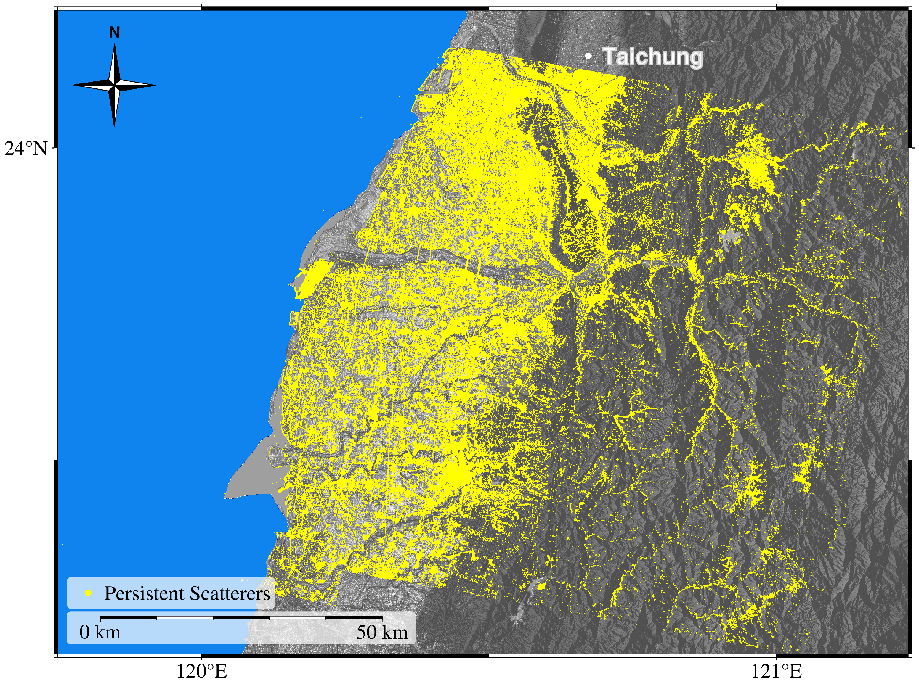
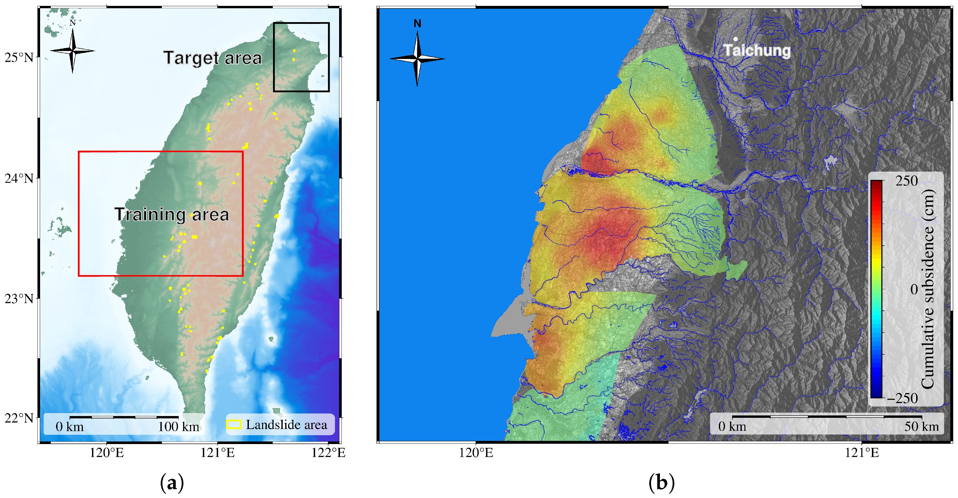
As a requirement for supervised learning, a study area located in central Taiwan is selected to generate the PSInSAR results for model training. Subsequently, a large-scale landslide area in northeastern Taiwan is chosen as the target site for the proposed PS pixel-selection approach. The area of interest is illustrated in Figure 1. An overview of Taiwan and the coverage of data used in model training, marked by the red rectangle, and the target area for application, indicated as the black rectangle. The yellow area is the location of large-scale landslides. The cumulative deformation until 2020 caused by land subsidence is shown in Figure 1b, while the blue line shows the river in this area.

In this work, the central Taiwan area is selected for the training dataset. This region encompasses plains, mountains, and hills, with characteristics reflective of both urban and rural areas. In addition, the land subsidence, caused by groundwater pumping for agricultural requirements, affects the region of the Choushui River alluvial fan, therefore exhibiting multi-temporal surface deformation signals in the PSInSAR result. Based on the long-term monitoring using Global Navigation Satellite System (GNSS) and precise leveling funded by the Water Resources Agency (WRA), Taiwan, about 190 cm of cumulative subsidence until 2020 is observed in Yunlin County, which is widely recognized as one of the regions most severely impacted by land subsidence. Several studies based on the DInSAR technique have also indicated up to 90 mm/yr subcidence over two decades. Due to governmental regulations on groundwater extraction, the severity of land subsidence has gradually diminished in recent years, with a deformation rate of about 50 mm/yr observed in a recent study [18,19].

The geohazard caused by slope activity and failure has attracted increasing attention in recent years, especially after the catastrophic Siaolin Village event triggered by typhoon Morakot in 2008. In Taiwan, numerous slopes, with mountainous settlements in the surrounding, have been identified by the Agency of Rural Development and Soil and Water Conservation as potentially active areas, which are delineated as yellow polygons in Figure 1a. Consequently, landslide monitoring using remote sensing techniques has emerged as an important and active area of research. Previous studies have indicated a good performance while using the PSInSAR technique for landslide activity monitoring [20,21,22], yet most cases have enough PS density for deformation analysis because of existing buildings or low vegetation coverage. The difficulty of long-term deformation analysis in areas with vegetation coverage persists, resulting in low quality, or even no observations [23].

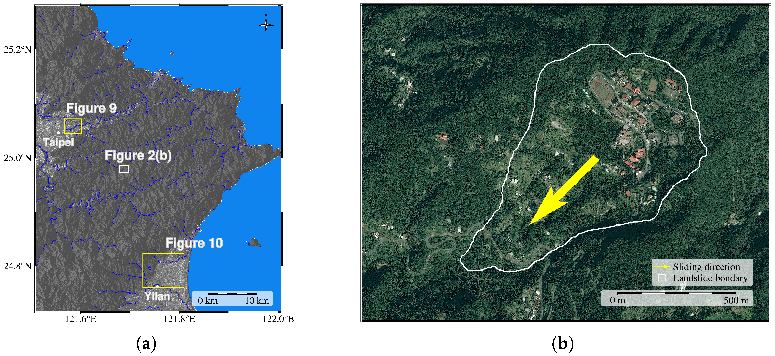
In order to apply and validate the performance of the model classification of Persistent Scatterers in an area with low coherence, the large-scale landslide located at Shiding District, New Taipei City, northern Taiwan, is selected as the target for analysis of the deformation caused by slope activity. The coverage of the InSAR dataset is shown in Figure 2a. The target landslide, which is indicated as a white rectangle in Figure 2a, is sloping toward the southwest with an approximately 20° dip angle. This area has become an outstanding site for landslide and geohazard research in recent years, as the campus of Huafan University is located on and seriously affected by the active slope. Previous studies have indicated creeping activity of about 20–30 mm/yr along the sliding surface, which is supposed to be 30–40 m underground based on on-site inclinometer monitoring [24]. In addition, 2 regions, including urban and field areas shown as yellow rectangles in Figure 2a, are selected to illustrate the ability of iDS prediction for a single pair interferogram. The white polygon in Figure 2b is the boundary of the landslide area identified by the Agency of Rural Development and Soil and Water Conservation.

2.2. Data

In this study, images from the ESA Sentinel-1 satellite are employed to analyze surface deformation and detect landslide activity. Sentinel-1 operates in Terrain Observation by Progressive Scans (TOPSAR) mode, acquiring imagery with a spatial resolution of 5 × 15 m with a swath width of 250 km, and a 12-day revisit cycle, making it appropriate for large-scale, long-term deformation monitoring at relatively high spatial resolution. 55 Sentinel-1 images covering central Taiwan, which were acquired between 5 November 2014 and 19 December 2017, are used to generate the PSInSAR dataset for model training. For the landslide application in northern Taiwan, 175 Sentinel-1 images are obtained and processed. These images used in the work are listed in

Table 1. Specifications for the SAR datasets applied in this study.

Study Area	Staellite	Orbit	Number of Images	Time Period
Central Taiwan	Sentinel-1	Descending	55	5 November 2014–19 December 2017
Northern Taiwan	Sentinel-1	Ascending	175	5 January 2019–28 December 2024

.

2.3. Methods

The rapid rise of deep learning methods for image recognition and classification has drawn considerable attention due to their substantial efficiency gains and high accuracy, and these methods have increasingly been applied to remote sensing imagery. Among them, the convolutional neural network (CNN) is one of the most widely used architectures, specifically designed to process grid-structured image data [25]. A conventional CNN architecture is composed of three main components: convolutional layers, pooling layers, and fully connected layers. Convolutional layers utilize learnable kernels to extract salient features from the input, while pooling layers downsample the feature maps to reduce dimensionality and computational cost, preserving critical information. Fully connected layers then integrate these features with class labels to perform image classification. Through this structure, CNNs enable automated feature extraction and reduce the reliance on hand-crafted features [26].

Conventional CNNs typically assign a single label to an entire image. However, many recognition tasks, particularly in remote sensing, require pixel-level classification to capture the spatial distribution of different classes. For such a purpose, Fully Convolutional Networks (FCNs) were introduced to provide a deep-learning-based method of pixel-based classification. Unlike CNNs, which require input images of fixed size, FCNs can accept inputs of arbitrary size, making them suitable for images with large dimensions. By upsampling or transposed convolution layers, FCNs map extracted feature representations back to the original resolution, producing dense, pixel-level predictions [27].

On this basis, Ronneberger et al. [28] proposed that the U-Net architecture, named for its characteristic U-shaped structure, was initially designed for biomedical image segmentation and has become one of the most effective models for pixel-level prediction. Compared with standard FCNs, U-Net offers superior edge localization and requires fewer training samples, making it especially suitable for applications with limited labeled data. Its architecture consists of a contracting path, composed of convolutional and pooling layers for hierarchical feature extraction, and an expansive path, consisting of upsampling, deconvolutional, and convolutional layers, which enables precise spatial localization through feature map fusion. In practical implementation, large-scale remote sensing images are subdivided into smaller overlapping tiles for training and inference, which allows efficient processing under limited GPU memory. The fully convolutional nature of U-Net enables seamless tiling and reconstruction without requiring fixed input dimensions. Tiles, after applying the classification procedure, are then seamlessly stitched together to generate a complete prediction map.

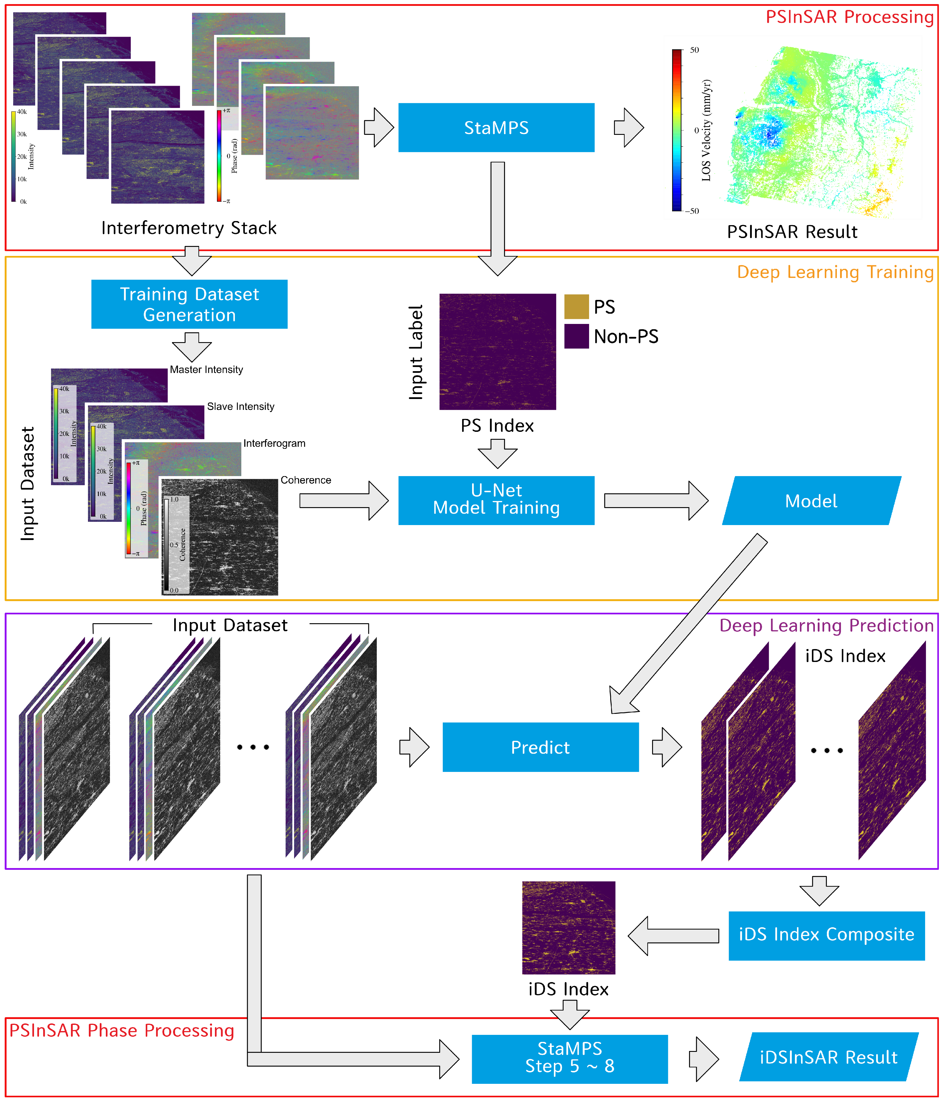
From a deep learning perspective, which naturally aligns with the dense prediction capability of U-Net, PS identification can be formulated as a pixel-wise binary classification problem, where each SAR pixel is assigned to either the PS or non-PS class based on its temporal intensity and phase stability characteristics. Consequently, the U-Net architecture can be directly employed for iDS classification without modification. A newly designed data processing workflow is proposed in this study, shown in Figure 3, which consists of three stages: (i) generation of PSInSAR training datasets, (ii) training of the U-Net model using the generated datasets, and (iii) applying the U-Net model to a new interferometry stack.

2.4. Data Processing

2.4.1. PSInSAR Processing

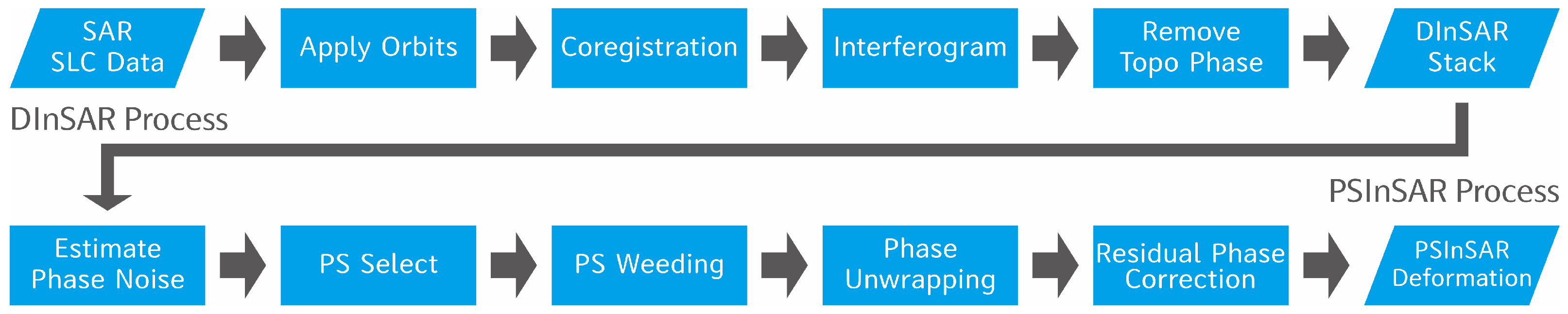
To utilize supervised training for a deep-learning-based model, which is optimized for Persistent Scatterer selection, a complete PSInSAR dataset with reasonable PS selection is necessary. In this study, three software packages were employed: SNAP for DInSAR preprocessing, StaMPS for persistent scatterer identification and phase error correction, and SNAPHU for phase unwrapping after PS selection. The standard PSInSAR procedure introduced by Hooper [29], as illustrated in Figure 4, is applied to the land subsidence area in central Taiwan. This approach starts from the interferograms with topographic and orbital phases removed. For the x-th pixel of the i-th interferogram, the residual phase can be expressed as:

$${\varphi }_{i,x}={\varphi }_{defo,i,x}+\Delta {\varphi }_{topo,i,x}+\Delta {\varphi }_{orbit,i,x}+{\varphi }_{atm,i,x}+{\varphi }_{noise,i,x}$$

(1)

where $\varphi$ is the residual phase, ${\varphi }_{defo}$ is the phase difference caused by deformation along satellite line-of-sight (LOS) direction, $\Delta {\varphi }_{topo}$ is residual phase because of the topographic error in the input digital elevation model (DEM), $\Delta {\varphi }_{orbit}$ is the residual phase due to the satellite ephemeris inaccuracies, ${\varphi }_{atm}$ is a phase caused by the atmospheric phase delay between acquisitions, and ${\varphi }_{noise}$ is from background noise.

In the StaMPS framework, an initial screening based on amplitude dispersion was applied prior to phase stability analysis. Pixels with a low Amplitude Dispersion Index are selected as Persistent Scatterer Candidates (PSCs) and are then subjected to phase stability analysis. The Amplitude Dispersion Index is defined by Ferretti [2] as:

$$D_A={\displaystyle \frac{{\sigma }_A}{{\mu }_A}}$$

(2)

For every PSC, spatially correlated phase components, such as atmospheric and orbital effects, are iteratively estimated and separated from temporally incoherent noise. Assuming that the DEM error can be modeled as a function of perpendicular baseline, the phase stability of each pixel can be evaluated by analyzing the dispersion of the residual phase after removing the spatially averaged component and the estimated DEM error. Then, the phase stability measure is defined as the following formula:

$${\gamma }_x={\displaystyle \frac{1}{N}}\left|\sum _{i=1}^{N}exp\left\{j({\varphi }_{x,i}-{\overline{\varphi }}_{x,i}-\Delta {\widehat{\varphi }}_{ϵ,x,i})\right\}\right|$$

(3)

where N is the number of interferograms, ${\overline{\varphi }}_{x,i}$ represents the spatially averaged phase within a local neighborhood, and $\Delta {\widehat{\varphi }}_{ϵ,x,i}$ denotes the estimation of the topographic error term. Pixels exhibiting low phase dispersion are identified as persistent scatterers. To acquire a reasonable PS index for supervised training, the threshold of the Amplitude Dispersion Index is set to 0.4, and 1.0 is adopted for the weed standard deviation in StaMPS to remove pixels exhibiting high residual phase variance.

After identifying persistent scatterers based on phase stability, the residual phase components, which consist of deformation, DEM error, atmospheric delay, orbital errors, and noise, are iteratively estimated and separated following the StaMPS framework. The DEM error is modeled as a function of the perpendicular baseline and estimated through linear regression across the interferometric stack. Spatially correlated components are extracted using spatial low-pass filtering combined with temporal high-pass filtering and subsequently removed to suppress atmospheric effects and residual orbital errors. Consequently, a PS index, which will be used as the label for supervised training, can be extracted from the PSInSAR results in Central Taiwan, illustrated in Figure 5.

2.4.2. Model Training

A supervised learning framework was adopted to train the neural network using input data and PSInSAR-derived labels. Classification labels were derived directly from PSInSAR results, which divide SAR image pixels into two classes: PS and non-PS. This labeling strategy preserves the physical interpretation of persistent scatterers and avoids subjective bias from manual annotation. The traditional PSInSAR algorithm is based on statistical analysis in both temporal and spatial domains to identify PS points. To ensure the high reliability of identified PS points regardless of the number of available SAR acquisitions, the phase differences of selected PS pixel clusters should remain consistent across all observations. Generally, at least 15 SAR images are recommended to obtain stable PS estimates [30]. However, long temporal baselines increase the likelihood of decorrelation, leading to a gradual reduction in the number of eligible PS points. Such a limitation is particularly challenging in mountainous regions, where scatterers are naturally sparse.

In this work, we propose a strategy for iDS classification that relies solely on spatial backscattering and phase characteristics, independent of temporal continuity, thus increasing the density of iDS points within individual interferometric pairs, thereby improving the spatial accuracy of phase unwrapping. In vegetated regions, interferometric pairs that experience severe decorrelation due to vegetation growth cycles are discarded, while the remaining pairs still enable reliable estimation of long-term deformation trends. This strategy is designed to increase iDS density, thus improving the phase unwrapping accuracy.

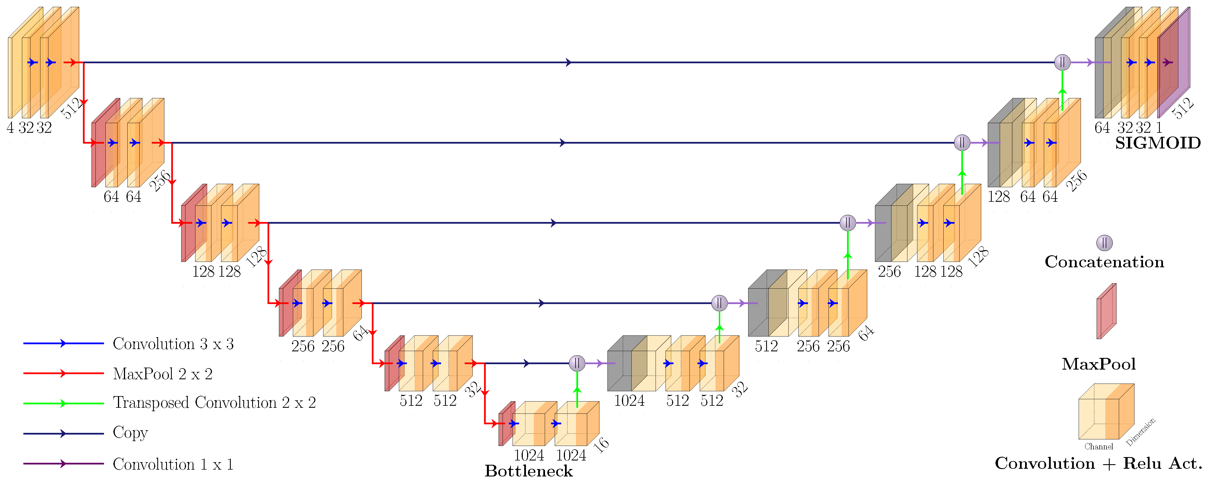
The architecture of the U-Net proposed in this work is shown in Figure 6. It is based on the original U-Net framework proposed by Olaf Ronneberger et al., consisting of a symmetric encoder–decoder structure with skip connections. The network comprises five downsampling stages followed by a bottleneck layer and five corresponding upsampling stages. The encoder progressively extracts hierarchical features using two consecutive 3 × 3 convolutional layers with ReLU activation at each level, followed by 2 × 2 max-pooling for spatial downsampling. The initial number of filters was set to 32 and doubled after each downsampling stage. Batch normalization was applied before each convolutional block from the second stage onward to improve training stability, and dropout (rate = 0.25) was introduced after deeper pooling layers to mitigate overfitting in deeper encoding and intermediate decoding stages. The bottleneck layer consists of two 3 × 3 convolutional layers with the highest filter depth. In the decoder, feature maps are upsampled using 2 × 2 transposed convolutions and concatenated with the corresponding encoder feature maps via skip connections. Each upsampling stage is followed by two 3 × 3 convolutional layers with ReLU activation, batch normalization, and dropout in intermediate decoding layers. The number of filters is halved at each decoding stage to maintain symmetry with the encoder. Finally, a 1 × 1 convolutional layer with sigmoid activation is applied to produce pixel-wise binary classification outputs for iDS and non-iDS categories. The model was implemented using TensorFlow [31] and optimized with the Adam algorithm proposed by Diederik P. Kingma and Jimmy Ba [32]. Binary cross-entropy was employed as the loss function for classification problems [33]. To enhance convergence stability and mitigate overfitting, an adaptive learning rate reduction strategy and early stopping mechanism were applied, following standard deep learning optimization practices [34]. Key training parameters, including input size, number of channels, batch size, optimizer settings, number of epochs, and early stopping criteria, are summarized in

Table 2. Key training parameters used in this study.

Parameter	Value
Input dimension	512 × 512
Input channels	4
Classes	2 (PS/non-PS)
Loss function	Binary Cross-Entropy
Optimizer	Adam
Initial learning rate	0.001
Learning rate scheduler	ReduceLROnPlateau
Batch size	5
Epochs	100
Early stopping	Patience = 20, min_delta = 1 × 10−4
Model selection criterion	Best validation loss

.

To balance GPU memory constraints and the scale of surface object features, the tile dimensions of input data were set to 512 × 512 × 4 (height, width, and channel). The four channels, corresponding to (i) the master image intensity, (ii) the slave image intensity, (iii) the interferogram, and (iv) the coherence map of an interferometric pair, are selected as input because PS identification in StaMPS relies primarily on intensity dispersion and phase stability analysis. Due to the relatively large spatial resolution of each tile and the associated GPU memory consumption during backpropagation, the batch size was set to 5 to prevent GPU memory overflow during training. This configuration represents a trade-off between computational efficiency and memory limitations while maintaining sufficient gradient stability for parameter optimization. Random sampling was applied to extract 10,200 tiles of size 512 × 512 (height × width) with a uniform spatial distribution from the co-registered DInSAR stack. The dataset was then divided into 10,000 training tiles and 200 validation tiles to evaluate model generalization during training. Subsequently, the input channels were generated by uniformly sampling a single interferometric pair from the total of 54 differential interferograms. Finally, sufficient training samples from a limited number of interferometric pairs are generated, incorporating temporal diversity that allows the model to learn features across different acquisition times.

The classification results are represented as a 512 × 512 × 1 output matrix, where the single channel indicates the probability of each pixel being an iDS point. Although the network generates a full-resolution output, only the central 384 × 384 region is retained for subsequent analysis. This cropping strategy is adopted to mitigate boundary effects introduced by convolutional operations and zero-padding near tile edges. Pixels located at tile margins have a reduced effective receptive field and are more susceptible to prediction uncertainty. By preserving only the central region, the influence of edge artifacts is minimized, thereby improving the reliability of iDS probability estimation. Eventually, pixels with predicted iDS probabilities greater than 0.1 were selected, generally indicating that phase-continuous regions are adequately captured for subsequent deformation analysis. The selection of this threshold is discussed in detail in Section 4.1, where its impact on classification performance and deformation reliability is systematically evaluated.

2.4.3. iDS Classification and Deformation Estimation

The study area includes several potential large-scale landslides in northern Taiwan. A total of 175 ascending Sentinel-1 images, acquired between 5 January 2019 and 28 December 2024, were processed. These images form 174 differential interferometric pairs, with the master image acquired on 9 October 2021. Each differential interferogram pair was classified using the trained U-Net model, producing 174 classification results.

This work aimed to replace the PS point classification step in the StaMPS software with a deep learning approach, while retaining other PSInSAR components for phase processing. The workflow integrates several classification outputs from interferograms in DInSAR stack into a unified iDS index, which is subsequently used for phase unwrapping, error estimation, and atmospheric phase filtering. Hence, the pixel-wise average of the classification probabilities across all predictions of interferogram pairs was calculated to generate a composite iDS index. Pixels with a probability greater than 0.1 were identified as iDS and imported into StaMPS for subsequent deformation analysis.

2.4.4. Evaluation Metrics

In order to quantitatively evaluate the performance of the neural network for pixel-wise binary classification of remote sensing imagery, several complementary evaluation metrics were adopted. These metrics are derived from the confusion matrix and are commonly used in both remote sensing and artificial intelligence literature to account for class imbalance and spatial prediction accuracy.

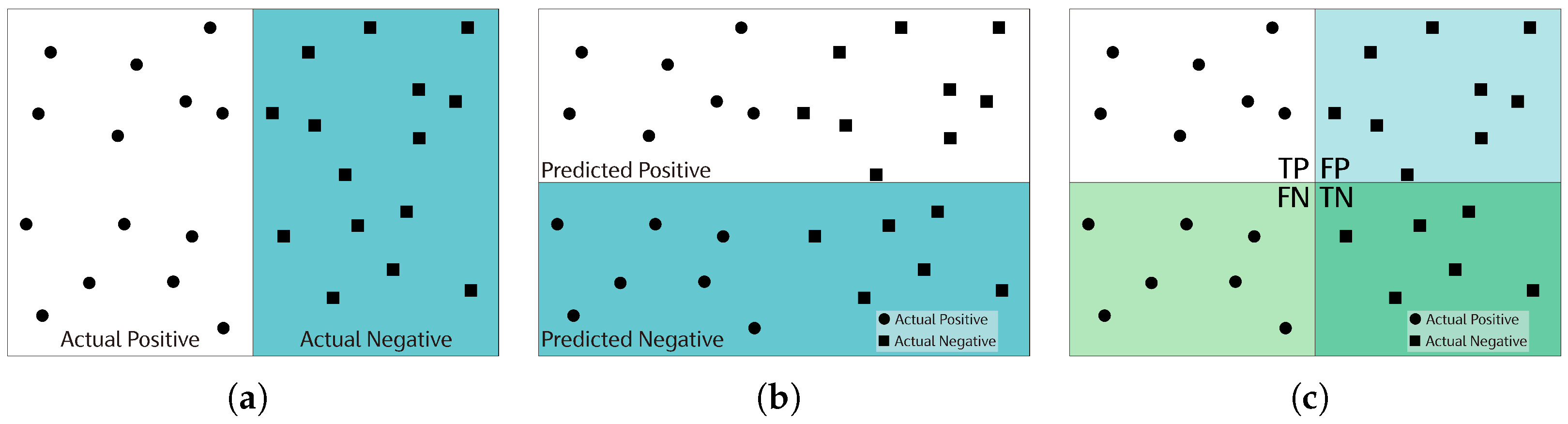
For a binary classification problem, the confusion matrix consists of four elements—true positives (TP), true negatives (TN), false positives (FP), and false negatives (FN)—which are illustrated in Figure 7. In the context of pixel-level remote sensing classification, TP and FN correspond to correctly and incorrectly detected target pixels, while TN and FP represent correctly and incorrectly classified background pixels, respectively.

Based on these elements in the confusion matrix, several metrics are introduced to evaluate the performance of the model prediction. The Overall Accuracy, which measures the proportion of correctly classified pixels over the entire validation dataset, is defined as:

$$Accuracy={\displaystyle \frac{TP+TN}{TP+TN+FN+FP}}$$

(4)

Although overall accuracy provides an intuitive measure of global classification performance [35], it can be biased in the presence of class imbalance, which is common in remote sensing applications [36,37]. In this work, iDS classification constitutes a highly imbalanced binary classification problem, as iDS pixels typically account for only a small fraction of the total pixels compared to non-iDS pixels. Therefore, evaluation metrics that are more sensitive to class imbalance are adopted to provide a reliable validation of classification performance. Precision, Recall, True Negative Rate(TNR, also known as Specificity), and F1-score, which are frequently used in such scenarios, are defined as follows:

$$Precision={\displaystyle \frac{TP}{TP+FP}}$$

(5)

$$Recall={\displaystyle \frac{TP}{TP+FN}}$$

(6)

$$Specificity={\displaystyle \frac{TN}{TN+FP}}$$

(7)

$$F1-score=2\times {\displaystyle \frac{Precision\times Recall}{Precision+Recall}}$$

(8)

Precision reflects the reliability of the classifier when assigning a pixel to the positive class. A high Precision value indicates that the number of false positives is limited, implying that most pixels labeled as positive by the model correspond to true positive samples. In iDS classification, Precision is particularly important for controlling false alarms, where non-PS pixels may be incorrectly classified as iDS pixels. Recall quantifies the proportion of true positive pixels that are correctly detected by the classifier. It evaluates the model’s ability to capture all reference positive samples and is therefore closely related to the missed detection rate. A high Recall value suggests that only a small fraction of true positive pixels are overlooked. In imbalanced datasets, Recall is essential for assessing whether the minority class can be sufficiently detected, especially in applications where missing target pixels may significantly affect subsequent analysis. Specificity measures the proportion of true negative pixels that are correctly identified by the classifier. In the context of iDS classification, Specificity evaluates the model’s ability to correctly reject non-iDS pixels and thus reflects its robustness against false alarms. A high TNR value indicates that the network effectively suppresses misclassification of background or decorrelated pixels as iDS candidates. The F1-score is defined as the harmonic mean of Precision and Recall and provides a balanced measure of classification performance by jointly considering false positives and false negatives. A higher F1-score indicates that the model achieves a favorable trade-off between detection completeness and classification reliability. Compared with Overall Accuracy, the F1-score is less sensitive to class imbalance and explicitly accounts for the trade-off between Precision and Recall. Consequently, it serves as a comprehensive indicator of the classifier’s effectiveness in pixel-wise binary classification tasks, where both detection reliability and completeness are critical.

Together, Precision, Recall, Specificity, and F1-score provide complementary insights into classification performance. Their combined use enables a more informative and application-oriented evaluation of neural network-based pixel-level remote sensing classification models under imbalanced conditions. Moreover, these metrics can serve as a standard baseline for neural network selection and model tuning in subsequent studies.

3. Results

3.1. Training Performance

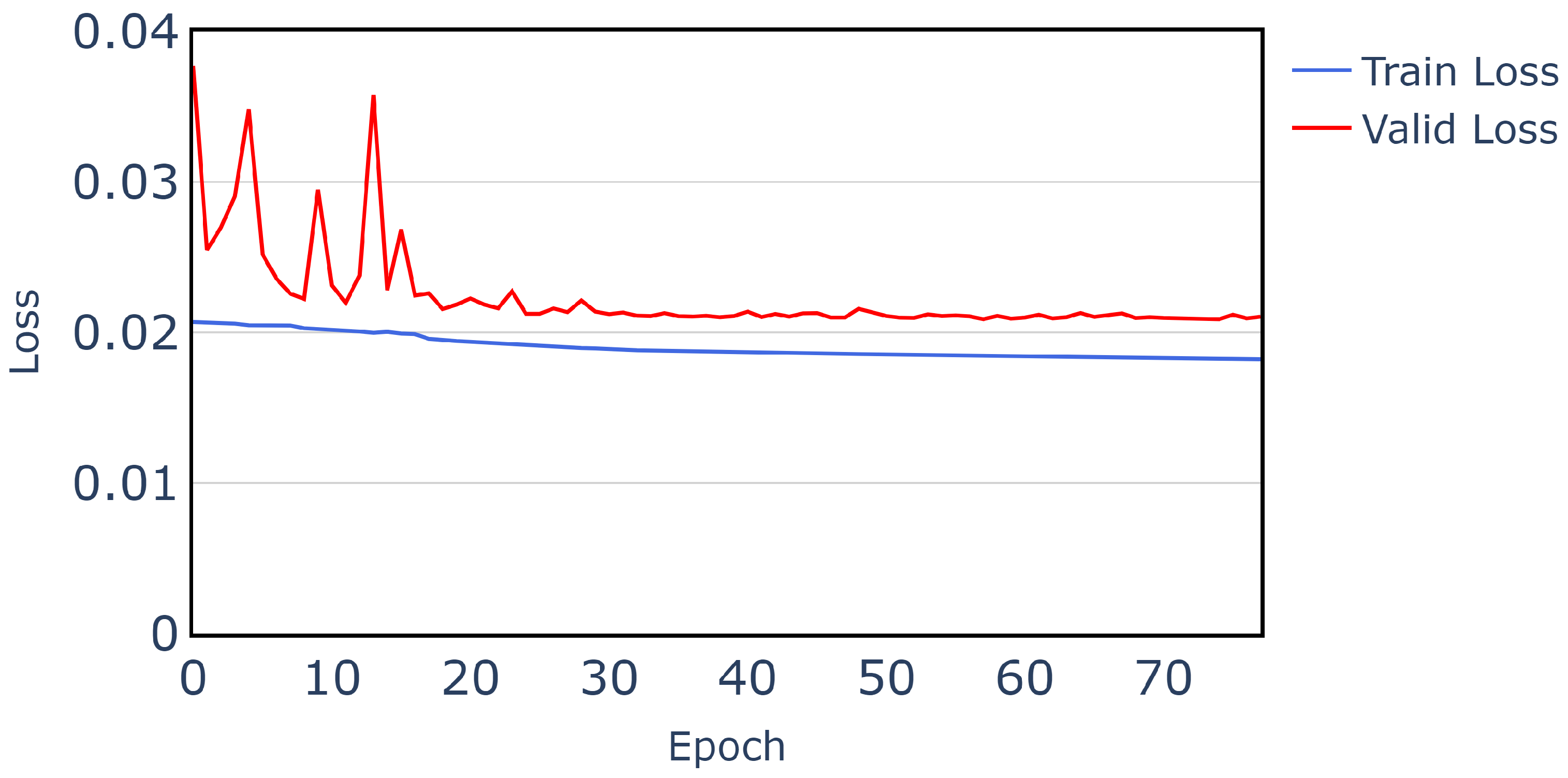
The training and validation loss curves of the proposed U-Net model are illustrated in Figure 8. The training loss gradually decreases during the training process, indicating stable model convergence. The validation loss exhibits relatively larger fluctuations in the early training stage, which can be attributed to the stochastic nature of mini-batch optimization and the relatively small validation set. After approximately 20 epochs, the validation loss stabilizes and follows a trend similar to that of the training loss, suggesting that the model achieves consistent generalization performance without significant overfitting. The final training and validation losses converge to approximately 0.018 and 0.021, respectively, demonstrating that the network effectively learns discriminative features for iDS identification.

3.2. iDS Results

In this section, four interferometric pairs characterized by different perpendicular and temporal baselines, as well as distinct seasonal conditions, were selected to evaluate the prediction performance of the proposed neural network. The corresponding iDS indices were generated for each interferogram to illustrate the model outputs. The selected interferogram segments are summarized in

Table 3. The segments of selected interferograms.

Slave Date	${\mathit{B}}_{\mathit{prep}}$ (m)	${\mathit{B}}_{\mathit{temp}}$ (Days)	Scenario
22 August 2021	25.19	−48	Wet season
2 November 2021	64.40	24	Dry season
22 September 2022	323.10	348	Perpendicular baseline
10 November 2024	−27.45	1128	Temporal baseline

.

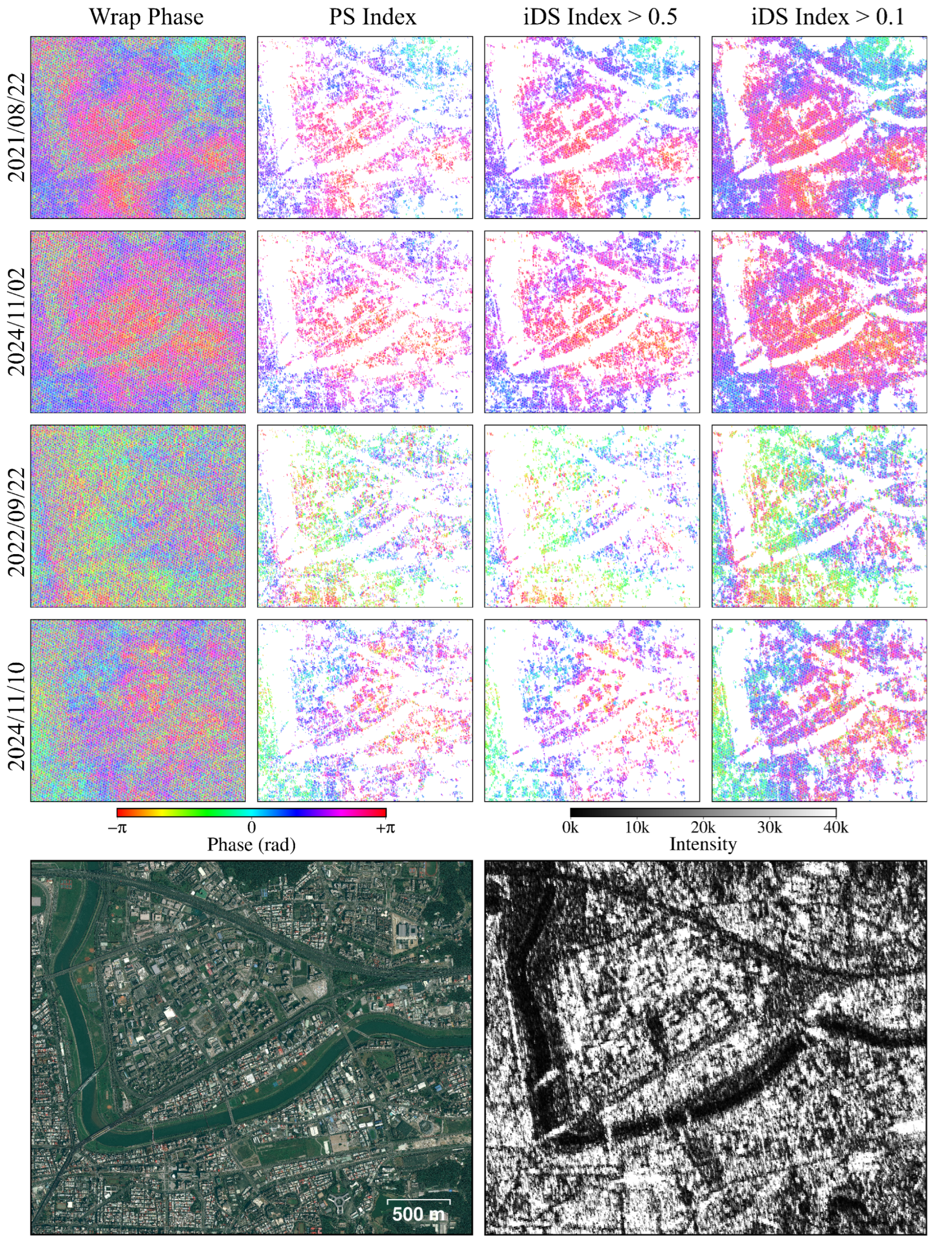
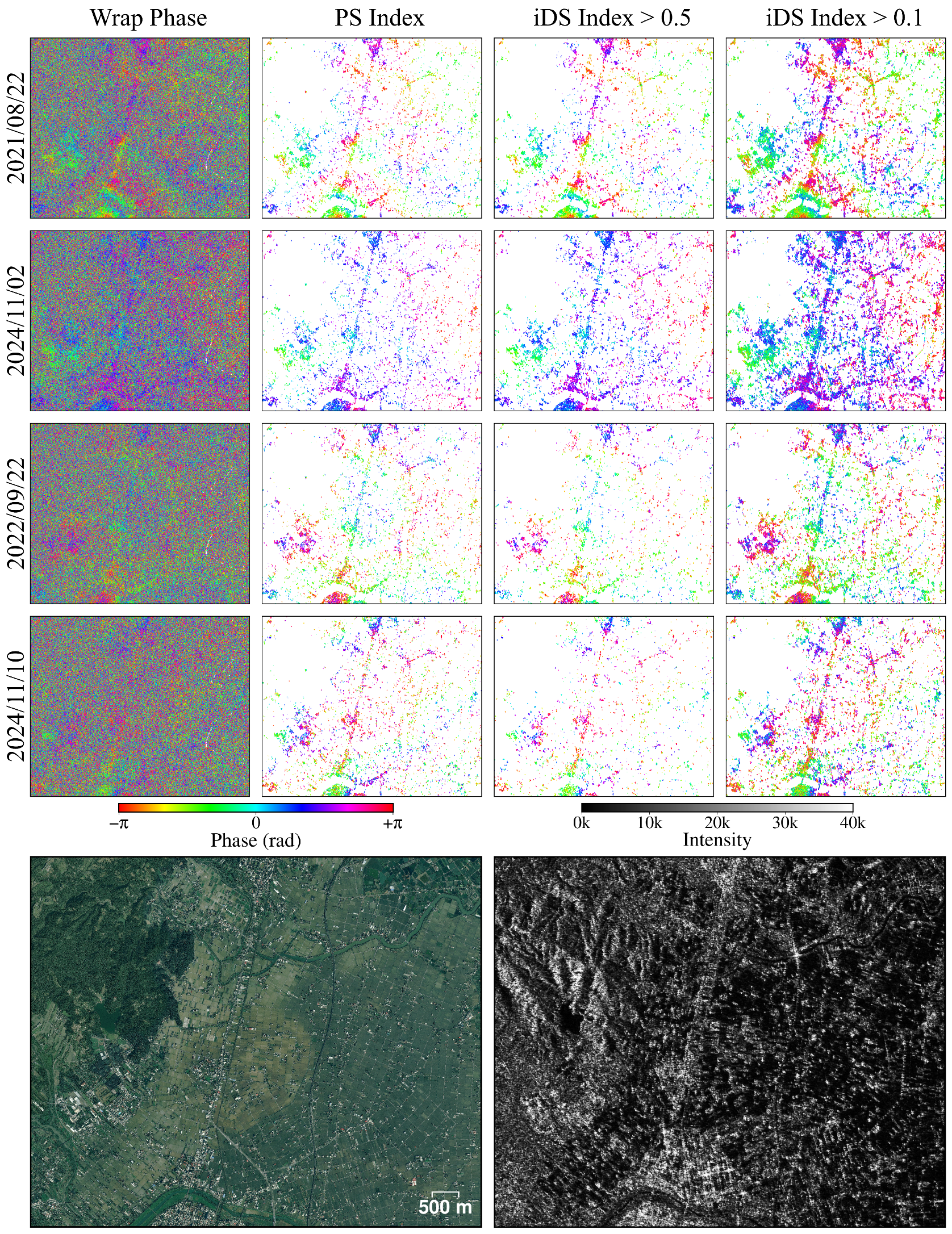
The iDS index was applied to interferograms to extract wrapped phase features in both the urban and field regions shown in Figure 2 with yellow rectangles. The urban area in the eastern part of Taipei City is characterized by rivers, high-rise buildings, and bridges, whereas the field region is located in northern Yilan County, with farms, fishponds, and mountains. The original interferogram and the PS index derived from PSInSAR were used to compare with the iDS index, and results are presented in Figure 9 and Figure 10, which include a 0.7 m resolution optical image acquired by the Pleiades satellite and the master SAR intensity image for reference of ground features. To evaluate the influence of probability threshold selection, two classification thresholds (0.5 and 0.1) were applied to the iDS index.

When a threshold of 0.5 was adopted, the spatial distribution of iDSs was generally consistent with the PS distribution derived from the StaMPS algorithm in two cases, which means pixels exhibiting stable phase behavior were successfully identified by the neural network. In the scenario of short perpendicular or temporal baselines, the iDS represents an increase because of the higher coherence compared to the large baselines case. However, with relatively large perpendicular or temporal baseline pairs, the density of iDS obtained by a threshold of 0.5 was a little less than the PS classification. These results indicate that the proposed neural network-based approach is capable of identifying distributed scatterers for a single interferometric pair in different correlation configurations.

Due to the slight decrease in iDS density in the large baseline scenario, a threshold of 0.1 was used to extract the wrapped phase and compare it with the case with a threshold of 0.5. The experimental results show that a dense distributed scatterer index, reflecting the increased detection of pixels with homogeneous phase characteristics, was obtained. In addition, several bridge structures in the Taipei case were detected under this relaxed threshold, whereas these objects were not identified in the PSInSAR-derived PS index due to temporal correlation issues.

Another example, applied in the field and mountain region, is selected to evaluate the performance of the proposed method in different ground characteristics. Beyond the usual downtown area, the results indicate that the distributed scatterers from the dispersed building in the field are identified as well. Furthermore, a lower threshold extends the coverage of existing iDS with a threshold of 0.1, and the neighboring iDS are characterized by a similar wrapped phase.

In summary, the wrapped phase extracted from the iDS index exhibits good quality and supports obtaining a better phase-wrapping result. A 0.5 threshold can provide an index consistent with the PSInSAR, while a lower 0.1 threshold demonstrates a similar wrapped phase with more distributed scatterers, which are considered to improve the precision of the phase wrapping procedure. Consequently, Pixels over the vegetation and water surface region are excluded in both cases, indicating the predictions from the deep-learning-based approach work as expected.

3.3. PSInSAR Results

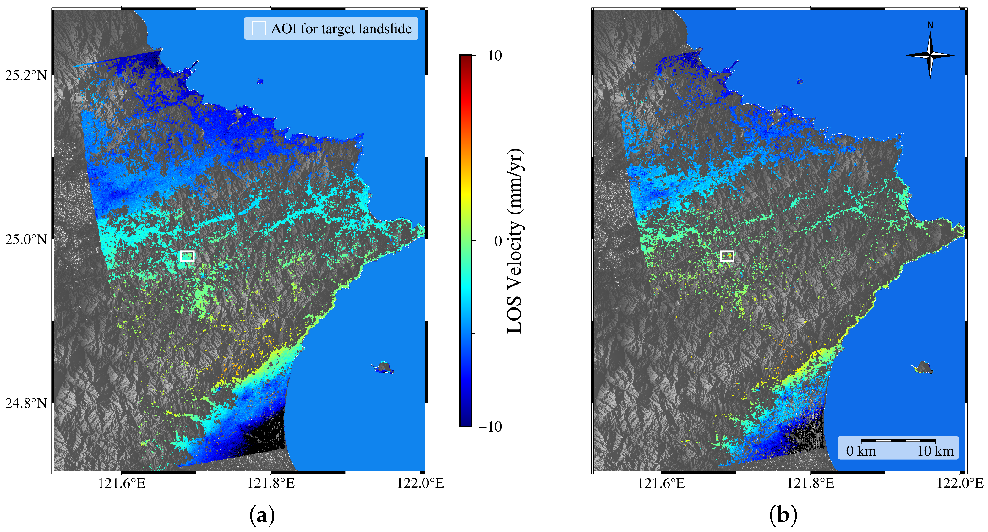
With 175 Sentinel-1 images and the proposed method described in Section 2, we obtained these PSInSAR measurements shown in Figure 11. The LOS velocity derived from the iDS index generated by the U-Net model, which shows a reasonable iDS distribution in northern Taiwan, is present in the left panel. For comparison, the PSInSAR LOS velocity from PSs predicted by StaMPS is also obtained and illustrated in the right panel. The white box marks the location of the large-scale landslide investigated in this study. The observations from two methods exhibit substantial similarity, and the spatial distribution of iDS pixels predicted by the U-Net model closely matches that of the StaMPS algorithm at the regional scale. These results demonstrate that deformation estimates based on the iDS index from U-Net prediction remain highly consistent with those derived from the conventional StaMPS workflow.

3.4. Large-Scale Landslide Monitoring

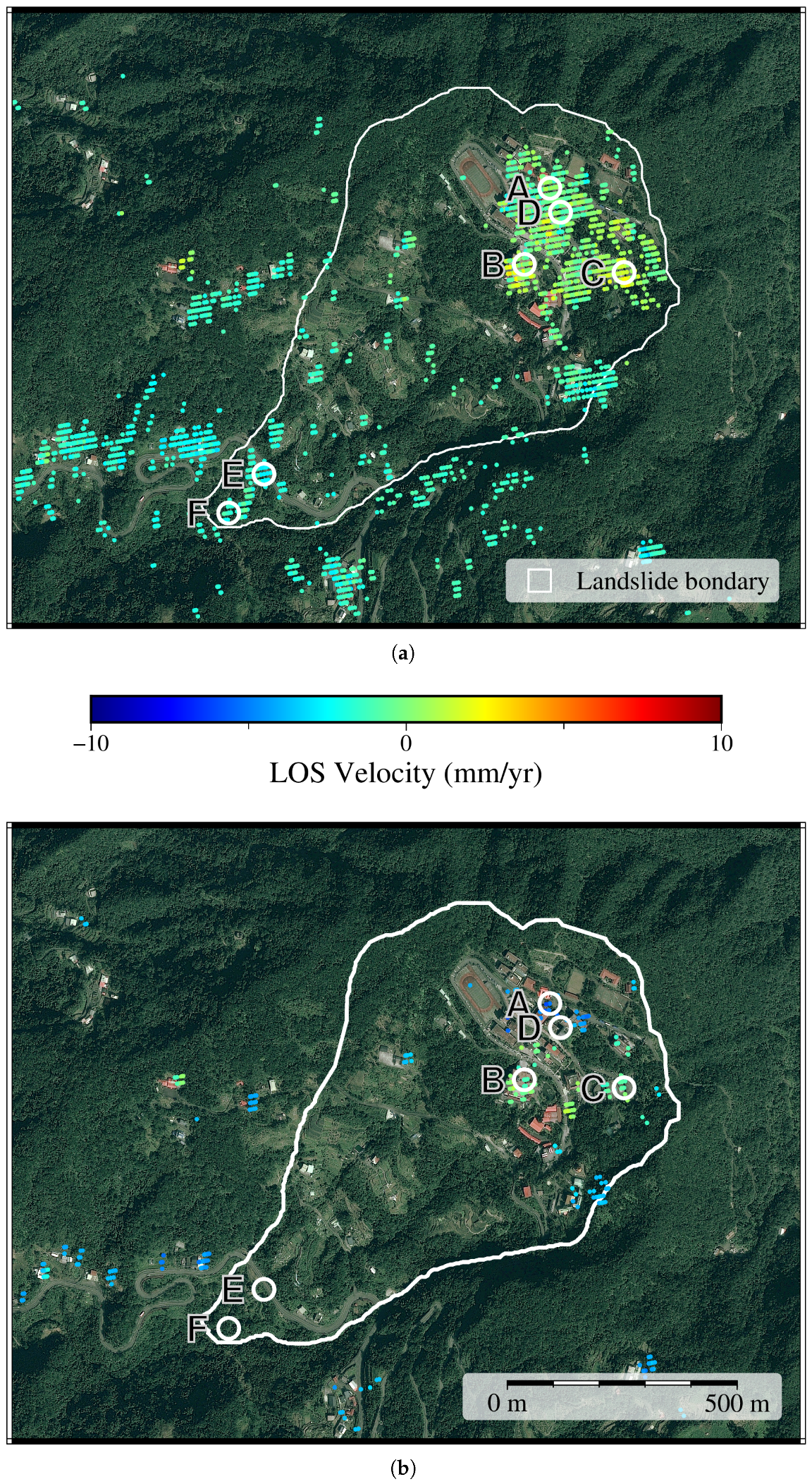
This session evaluated the performance of the new deep-learning-based method for iDS selection by applying it to PSInSAR deformation analysis in the potentially large-scale landslide area in northern Taiwan. The landslide areas were delineated primarily based on data published by the Agency of Rural Development and Soil and Water Conservation, MOA. The line-of-sight deformation rate of the landslide area is presented in Figure 12. The U-Net-derived iDS deformation analysis is shown in the upper column, while the StaMPS-derived results are in the lower. The boundary of the potentially large-scale landslide area is marked as the white polygon, and warm colors indicate surface uplift or motion toward the satellite. In contrast, cool colors symbolize subsidence or motion away from the satellite.

As a result, sparsely human-made structures in the head of the landslide area provide sporadic PS observations in the original PSInSAR analysis. Yet, the U-Net predictions not only capture iDSs from buildings more comprehensively but also identify additional iDSs at the foot of the landslide. As the slope faces southwest, deformation associated with slope activity can be detected as motion toward the satellite with ascending-orbit data. Accordingly, the results reveal buildings near the upper slope exhibiting velocities approaching the satellite, suggesting a potential trend of activity during the observation period. As a consequence, more observation points within the landslide area are obtained using the U-Net-based method, which demonstrates the capability of the proposed method compared to the result from StaMPS.

3.5. Time-Series Analysis

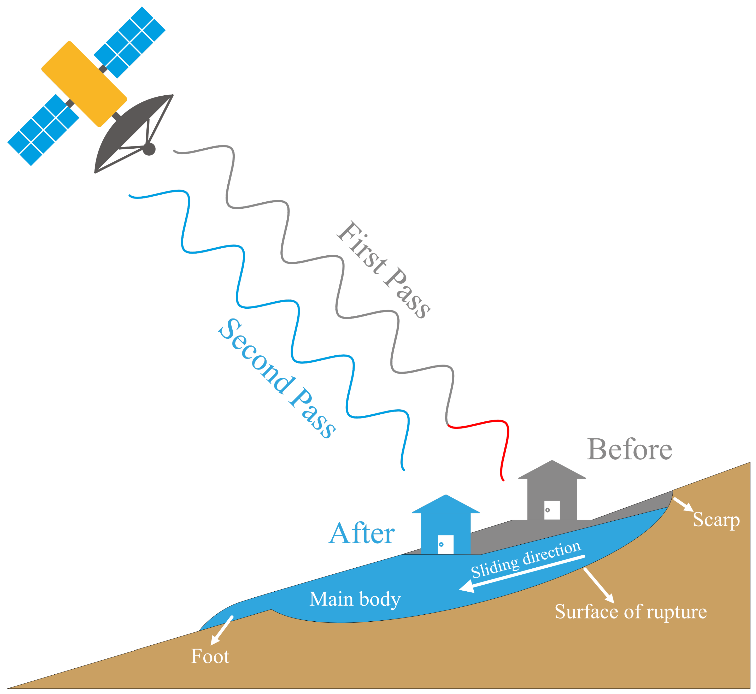
Several PSs identified within the landslide area were further analyzed using deformation time-series data. Because the deformation measurements were derived from SAR images acquired in an ascending orbit, the geometric relationship between the slope orientation and the satellite line-of-sight (LOS) direction must be considered. Under this geometry, slope activity causes movement toward the satellite and results in an apparent uplift signal due to the reduced distance between the satellite and the target. The geometric relationship between the satellite viewing direction and the landslide slope is illustrated in Figure 13.

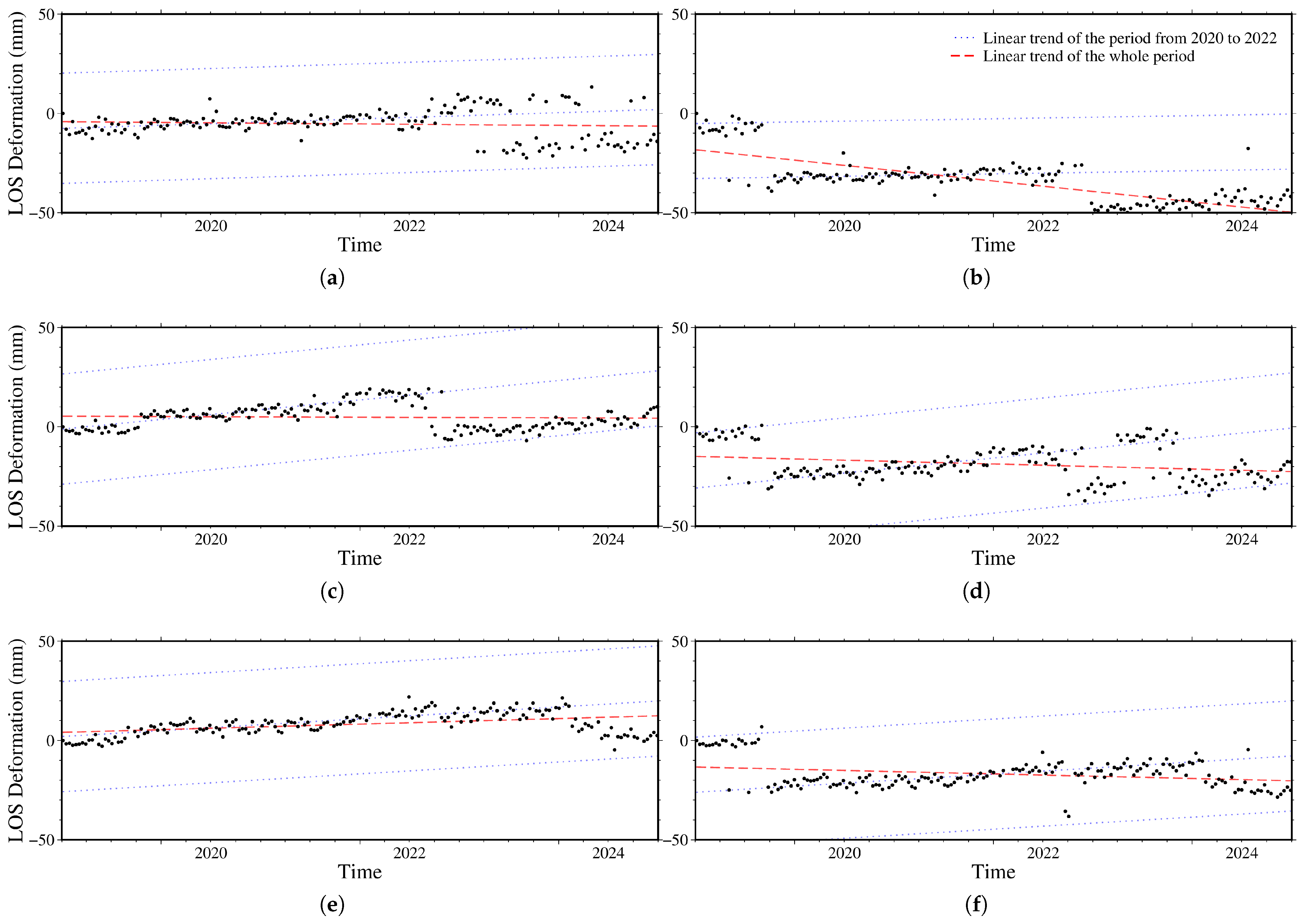
Three representative PS points (A, B, and C), located at different positions within the landslide area, are shown in Figure 12. These PSs were identified by both the proposed U-Net-based method and the conventional StaMPS approach. The deformation time series derived from both methods exhibits partially comparable trends, indicating long-term motion toward the satellite. Considering the slope geometry and satellite viewing direction, this apparent uplift can be interpreted as slope activity. However, the StaMPS-derived time series contains two significant offsets of approximately 27.73 mm, indicated by the blue dashed lines in Figure 14. These discontinuities result in an overall subsidence LOS velocity, which represents an unrealistic deformation behavior for the slope.

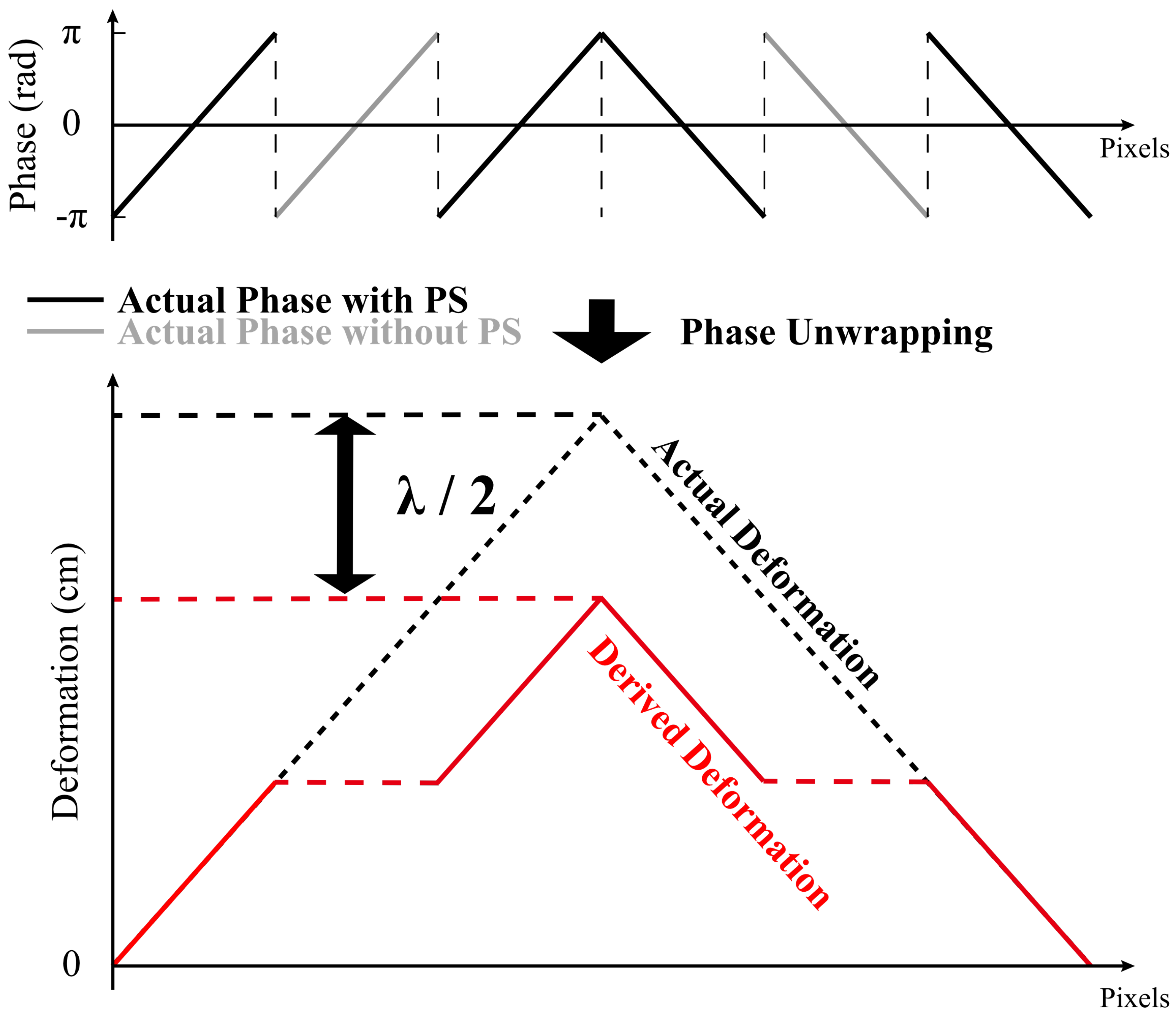
Previous studies have suggested that offsets of approximately 27.73 mm, corresponding to half of the wavelength of C-band SAR, are commonly associated with phase unwrapping errors [38]. Such errors may occur when spatial phase continuity is insufficient during the unwrapping process. As illustrated in Figure 15, the exclusion of numerous pixels in the PSInSAR processing stage can lead to spatial discontinuities in the phase field, resulting in phase ambiguity and subsequent unwrapping errors. These errors may cause underestimation or distortion of the LOS deformation velocity. Benefiting from the broader spatial distribution of identified distributed scatterers (iDSs), the U-Net-based approach provides a denser and more continuous set of phase observations. Consequently, the deformation time series derived from the proposed method exhibits fewer large offsets and a more stable deformation trend. The resulting regression-derived mean velocity, illustrated by the red dashed line in Figure 14, therefore provides a more reliable estimate of the long-term deformation behavior. These results support the idea that increasing the spatial density of stable scatterers from this U-Net-based approach can improve the spatial continuity of phase observations and thereby mitigate phase unwrapping ambiguities.

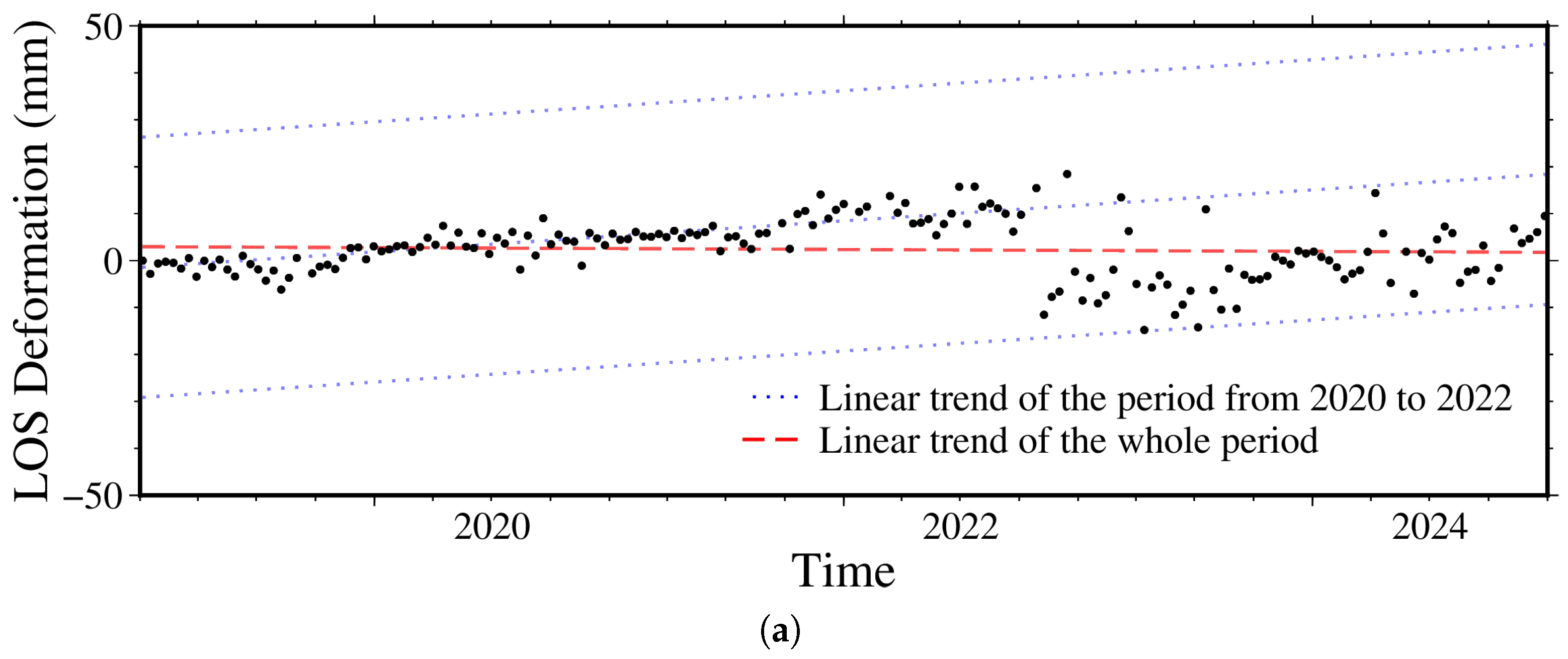
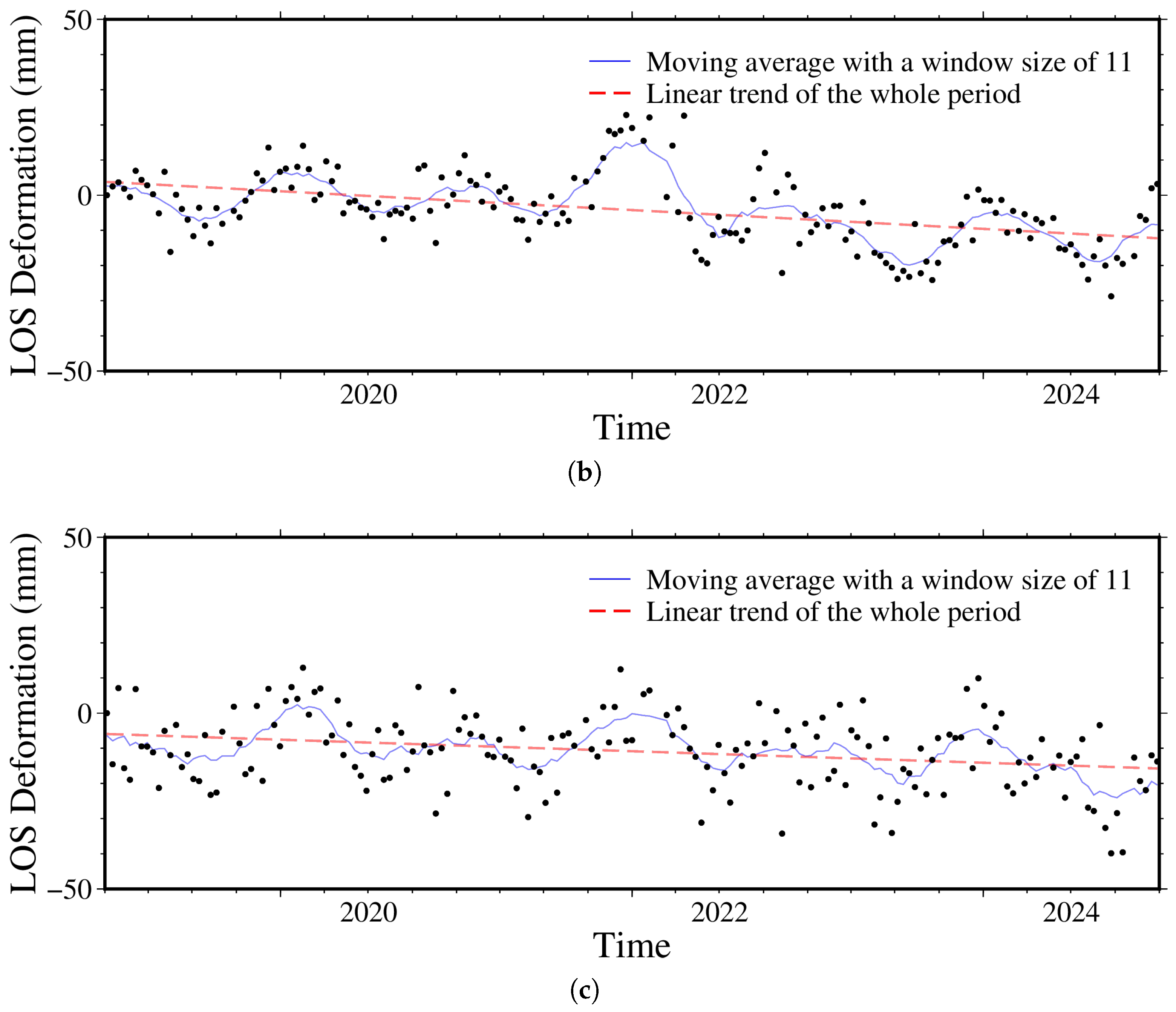
Additional iDS points (D, E, and F), which were detected only by the proposed U-Net method and therefore lack corresponding StaMPS results, are shown in Figure 16. iDS D is located on a campus building near the upper slope and exhibits a deformation pattern similar to that of iDS A, including indications of potential phase unwrapping disturbances. Although this target demonstrates persistent scattering characteristics for most of the observation period, it was excluded by the StaMPS processing due to insufficient phase stability. In contrast, iDS E and iDS F are located near the lower slope margin and exhibit seasonal fluctuations in their deformation time series, as indicated by the blue curves in Figure 16, while maintaining an overall stable long-term trend. These observations suggest that active deformation is primarily concentrated in the upper portion of the slope, whereas the lower slope remains relatively stable.

Overall, the results represent that the proposed method can detect iDSs that are dropped by StaMPS, thereby enhancing the density of observations and improving the assessment of surface deformation in areas with sparse PS coverage.

4. Discussion

4.1. Classification Validation

In order to evaluate the performance of the proposed neural network model for iDS prediction, a confusion-matrix-based validation was conducted for the case studies in Northern Taiwan. In this section, the predicted iDS index is compared pixel by pixel with the reference PS results generated by StaMPS, which serve as the benchmark for iDS classification in this study, producing a confusion matrix that characterizes four prediction scenarios. The confusion matrix for the IDS index, extracted at a probability threshold of 0.1, is listed in

Table 4. The confusion matrix of iDS classification in the Northern Taiwan area.

Method		StaMPS (Actual Class)
	Predict Class	Positive (PS)	Negative (Non-PS)
U-Net (Predicted Class)	Positive (iDS) Negative (non-iDS)	388,131 (TP) 31,295 (FN)	866,305 (FP) 50,714,269 (TN)

. The results confirm that the large number of true negative classes demonstrated by the catalog in the confusion matrix, about 97.39% of pixels in the interferogram stack are identified as non-iDS, while only about 2.61% are recognized as iDS by the neural network model.

Previous studies have shown that pixels located in ocean areas are consistently classified as non-PS due to low backscattering intensity and strong temporal phase decorrelation, which results in a large proportion of non-PS samples in the confusion matrix. This imbalance leads to an inflated overall accuracy and may obscure the actual classification performance of iDS detection. Consequently, ocean-area pixels were identified and excluded from the confusion matrix and subsequent performance analysis using elevation information derived from the DEM. The refined confusion matrix is summarized in

Table 5. The confusion matrix of iDS classification without ocean area.

Method		StaMPS (Actual Class)
	Predict Class	Positive (PS)	Negative (Non-PS)
U-Net (Predicted Class)	Positive (iDS) Negative (non-iDS)	383,919 (TP) 29,721 (FN)	846,242 (FP) 30,873,196 (TN)

.

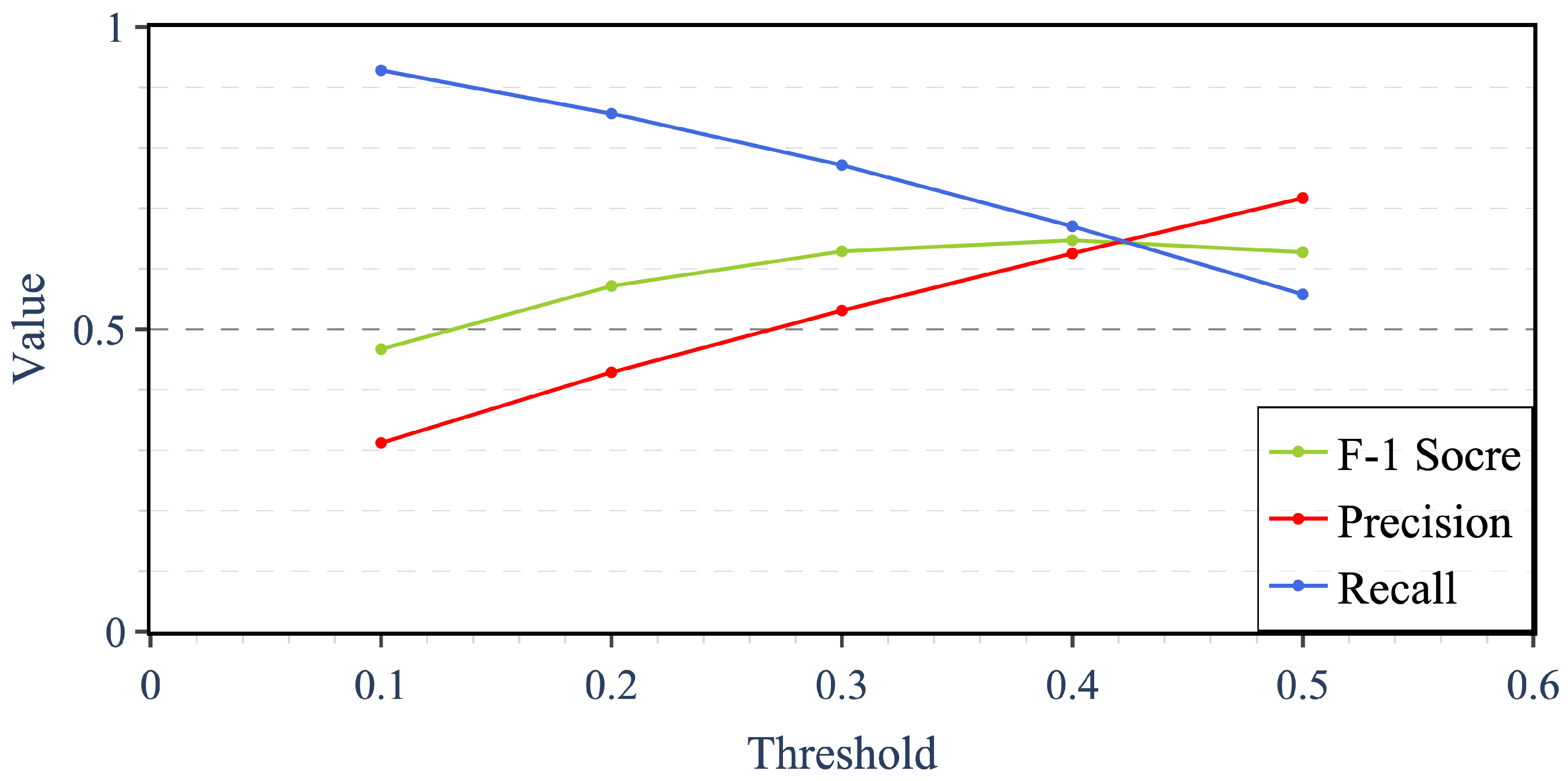
Based on this matrix, several standard evaluation metrics, including Accuracy, Precision, Recall, and F-1 score, can be derived to assess the classification performance of the trained model in this study. To choose a reasonable probability threshold, values between 0.1 and 0.5 are used to calculate the evaluation metrics. The corresponding values are summarized in

Table 6. The results of classification evaluation metrics.

Metrics		Score
	Threshold	0.1	0.2	0.3	0.4	0.5
Accuracy		0.9727	0.9835	0.9883	0.9906	0.9915
Precision		0.3121	0.4287	0.5309	0.6254	0.7169
Recall		0.9281	0.8566	0.7714	0.6703	0.5577
Specificity		0.9733	0.9851	0.9911	0.9948	0.9971
F-1 Score		0.4671	0.5715	0.6289	0.6471	0.6274

.

Although the overall accuracy reaches about 0.9 in every threshold setting, this metric alone does not adequately reflect predictive reliability because the classification in Table 5 illustrated a highly imbalanced distribution even after removing the pixel covering the ocean area, while the proportion of PS pixels relative to the total number of pixels on land is tiny.

In this context, the value of recall is the critical factor in this validation, as it represents the number of actual PSs correctly identified in the model prediction. A higher recall value indicates that most PSs are correctly identified by the neural network, demonstrating the model’s ability to preserve the stable scatterers identified by the conventional algorithm. In contrast, precision reflects the proportion of predicted iDS pixels that correspond to true PS pixels. In this study, precision is expected to decrease as additional iDS pixels are intentionally introduced, thereby increasing the commission error.

Figure 17 illustrates the effect of the probability threshold on the evaluation metrics. When the threshold is set to 0.5, the model achieves relatively high precision but at the cost of substantially reduced recall, indicating that approximately 45% of the actual PS pixels are omitted by the neural network. Conversely, lowering the threshold to 0.1 results in a relatively low precision value, which would typically be considered suboptimal in conventional classification tasks. The corresponding F1-score is also relatively low, reflecting an apparent imbalance between precision and recall under standard classification criteria.

Nevertheless, the results presented in Section 3.2 demonstrate that the threshold of 0.1 effectively identifies pixels with stable phase observations. As the primary objective of this approach is to introduce additional iDS pixels to enhance deformation monitoring in areas with low PS density, accepting a reduction in precision is a reasonable trade-off if it allows more PS pixels to be retained and reduces omission errors associated with the conventional algorithm. As a result, a value of 0.1 is selected as the threshold for obtaining the iDS index and further analysis.

It should be noted that the commission error in the iDS classification can introduce additional phase noise and increase the risk of phase unwrapping errors, resulting in a reduction in the precision of the deformation estimates. Accordingly, the major strategy in this work becomes to ensure that deformation observation derived by iDS from the neural network remains highly reliable, even though low precision and F-1 scores do not substantially affect the overall PSInSAR deformation trends.

4.2. Validation of Phase Stability

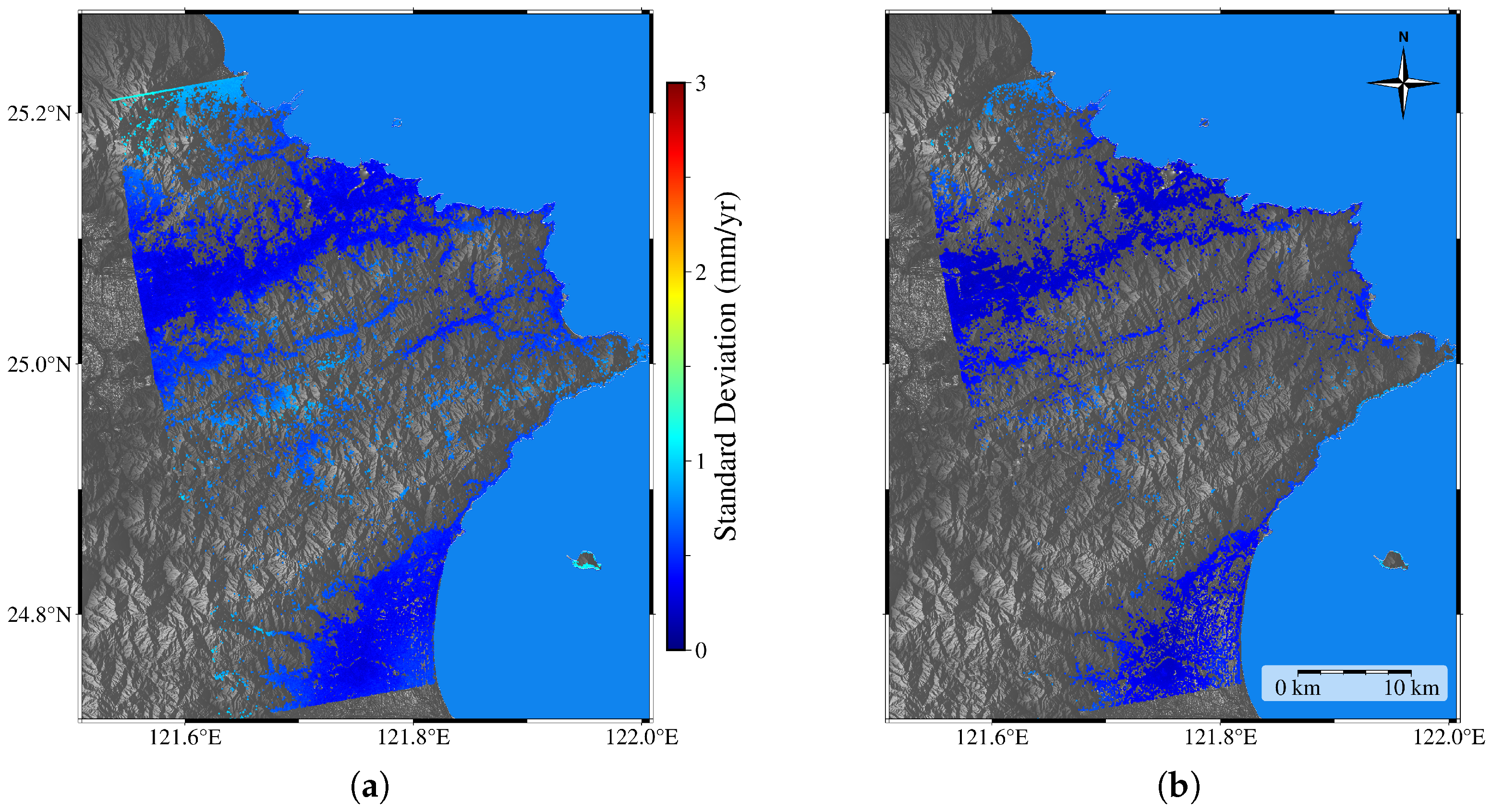
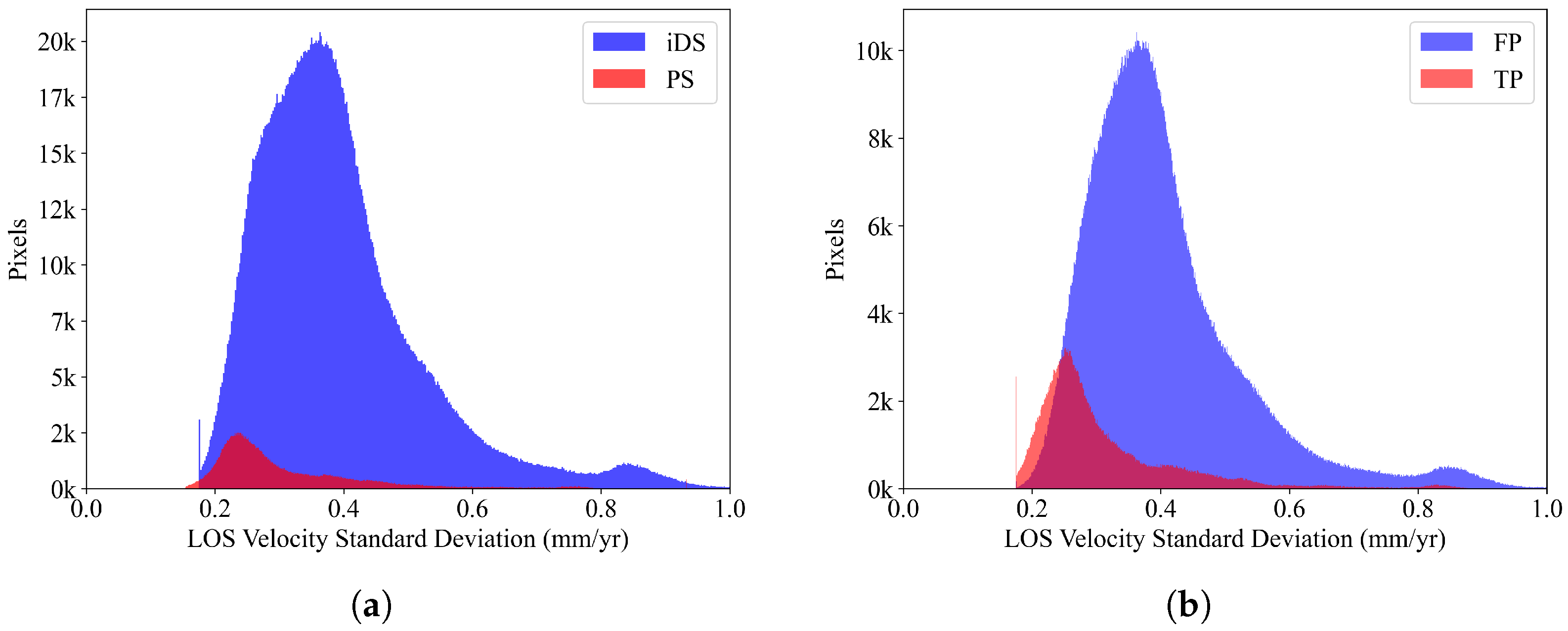
To assess the phase stability of the identified scatterers, the standard deviation of the line-of-sight velocity estimated from the StaMPS time-series analysis was first examined. The LOS velocity standard deviation reflects the uncertainty associated with the deformation rate derived from interferometric phase time series. As shown in Figure 18, pixels exhibiting stable phase behavior generally correspond to smaller velocity dispersion values. The histogram in Figure 19 compares the LOS velocity standard deviation for PS pixels identified by StaMPS and the iDS pixels predicted by the proposed U-Net model. The StaMPS-derived PS pixels are strongly concentrated within a low standard deviation range, indicating stable phase behavior and reliable deformation estimates. In contrast, the iDS pixels show a broader distribution with relatively larger velocity variability. This pattern is consistent with the intrinsic characteristics of persistent and distributed scatterers, where PS pixels typically exhibit higher temporal phase stability than distributed scatterers.

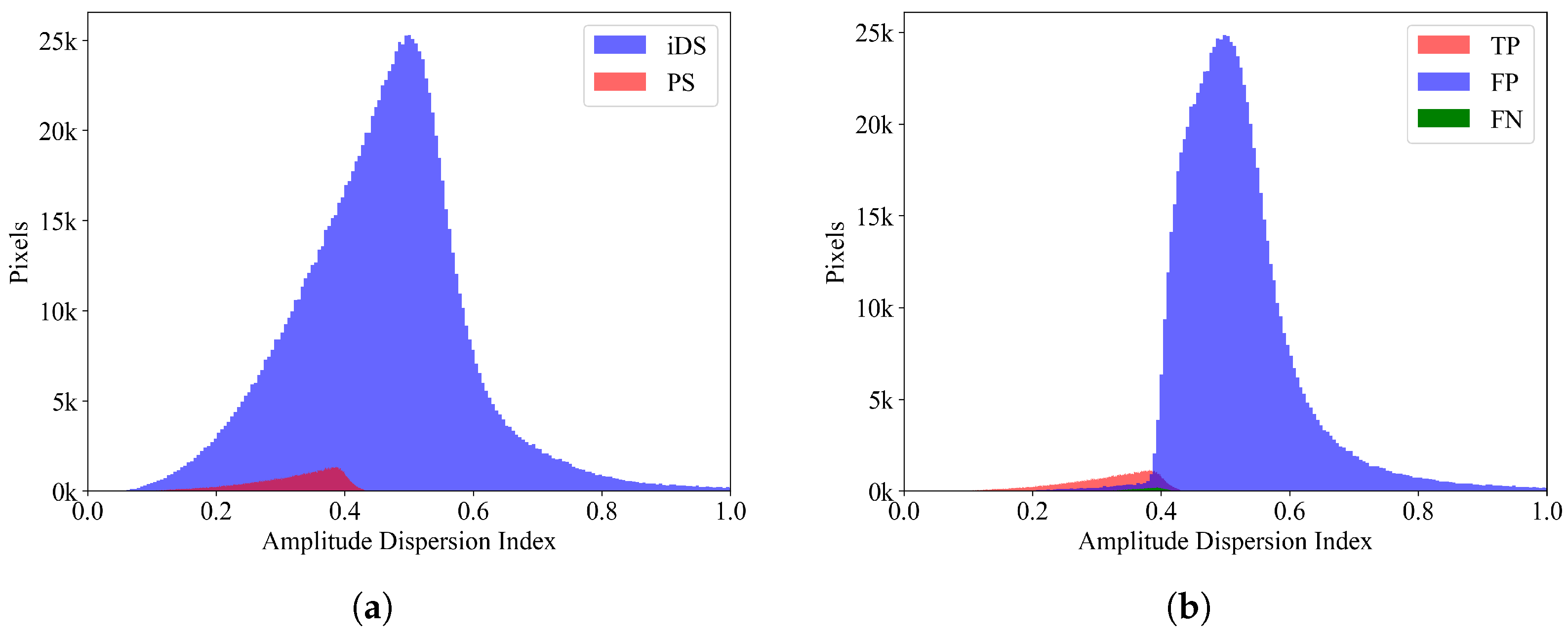
Amplitude stability was further evaluated using the Amplitude Dispersion Index (ADI), which is widely adopted in PSInSAR analysis as an indicator of temporal backscatter stability. The ADI is defined as the ratio of the standard deviation to the mean of the amplitude time series, where lower ADI values generally correspond to more stable scatterers and a higher likelihood of persistent scattering behavior [2]. Figure 20 shows the ADI distributions for the iDS pixels and the StaMPS-derived PS pixels. The PS pixels are primarily concentrated within lower ADI ranges, indicating stable amplitude behavior over time. In contrast, the iDS pixels exhibit a broader distribution with generally higher ADI values, consistent with the expected properties of distributed scatterers.

To further investigate the classification behavior of the U-Net model, the ADI distributions of true positives (TP), false positives (FP), and false negatives (FN) were analyzed. Most TP pixels are concentrated in the low-ADI region where PS pixels dominate. The FP pixels mainly occur within the transitional ADI range and introduce only a limited number of pixels with relatively high ADI values. This observation suggests that the misclassified pixels are primarily associated with scatterers exhibiting weaker amplitude stability. Overall, these results indicate that the U-Net model preserves the principal amplitude stability characteristics of persistent scatterers while introducing only a small proportion of higher-ADI pixels.

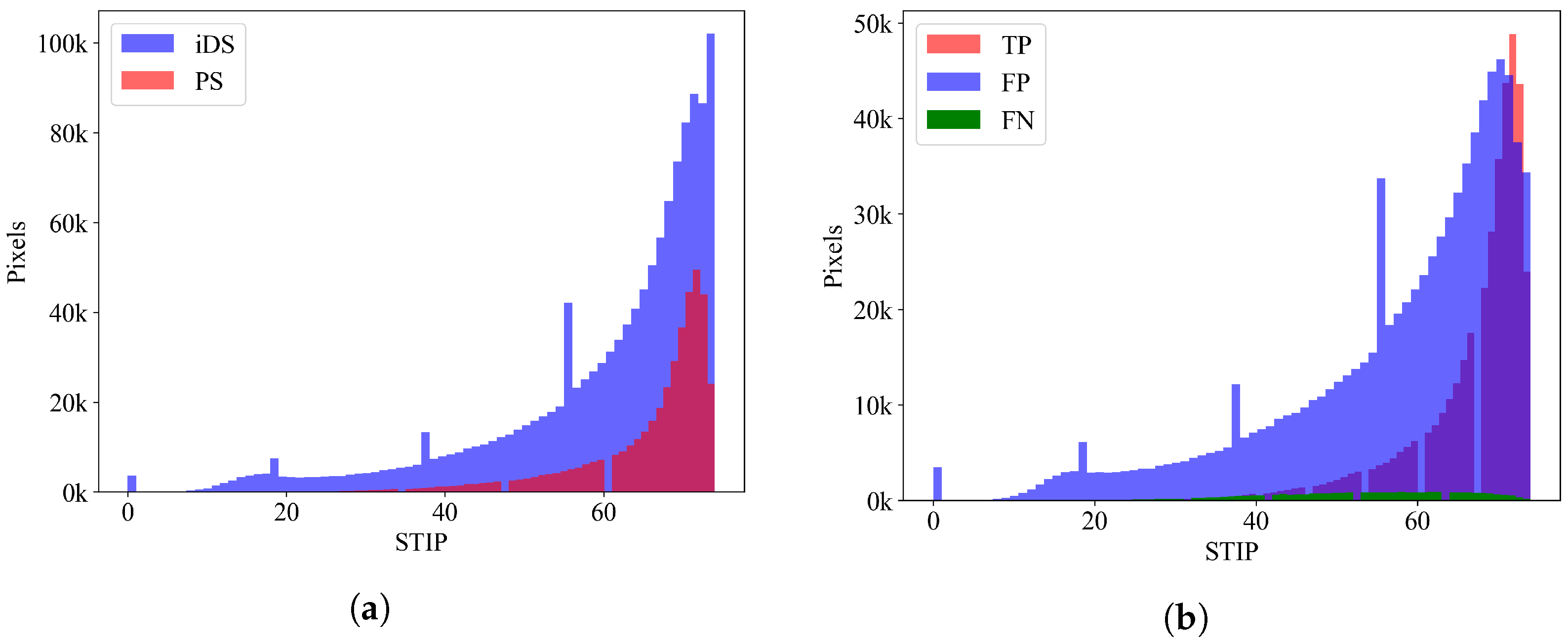
To analyze temporal phase stability, the Similar Time-series Interferometric Pixels (STIP) index was computed for all candidate pixels. The STIP index, proposed by Narayan et al., measures the number of neighboring pixels with highly similar interferometric phase time series within a local search window and serves as an effective indicator of phase stability. Higher STIP values correspond to lower phase noise and greater reliability for PSInSAR deformation monitoring [39]. Figure 21a illustrates the spatial distribution of STIP values across the study area. Compared with the StaMPS-derived PS pixels (red), the histogram of the iDS pixels (blue) exhibits a clear rightward shift, with a larger proportion of pixels concentrated in the high-STIP range (approximately 60–80). This result suggests that the deep learning-based selection identifies a greater number of pixels with strong temporal phase similarity than the conventional threshold-based StaMPS approach.

The STIP distributions for iDS pixels classified according to the confusion matrix are further shown in Figure 21b. The TP component dominates the high-STIP region, indicating that most high-stability pixels identified by StaMPS are successfully preserved by the U-Net model. Notably, a substantial portion of FP pixels also exhibits relatively high STIP values. This observation implies that many of these additional iDS pixels may possess comparable or even superior phase stability to those selected by StaMPS and could represent valid persistent scatterers that were not identified by the conventional algorithm due to amplitude or decorrelation constraints. Taken together, these results demonstrate that the proposed U-Net-based iDS approach not only increases the density of selected scatterers but also improves the overall phase quality of the pixel ensemble, as reflected by the enhanced STIP statistics.

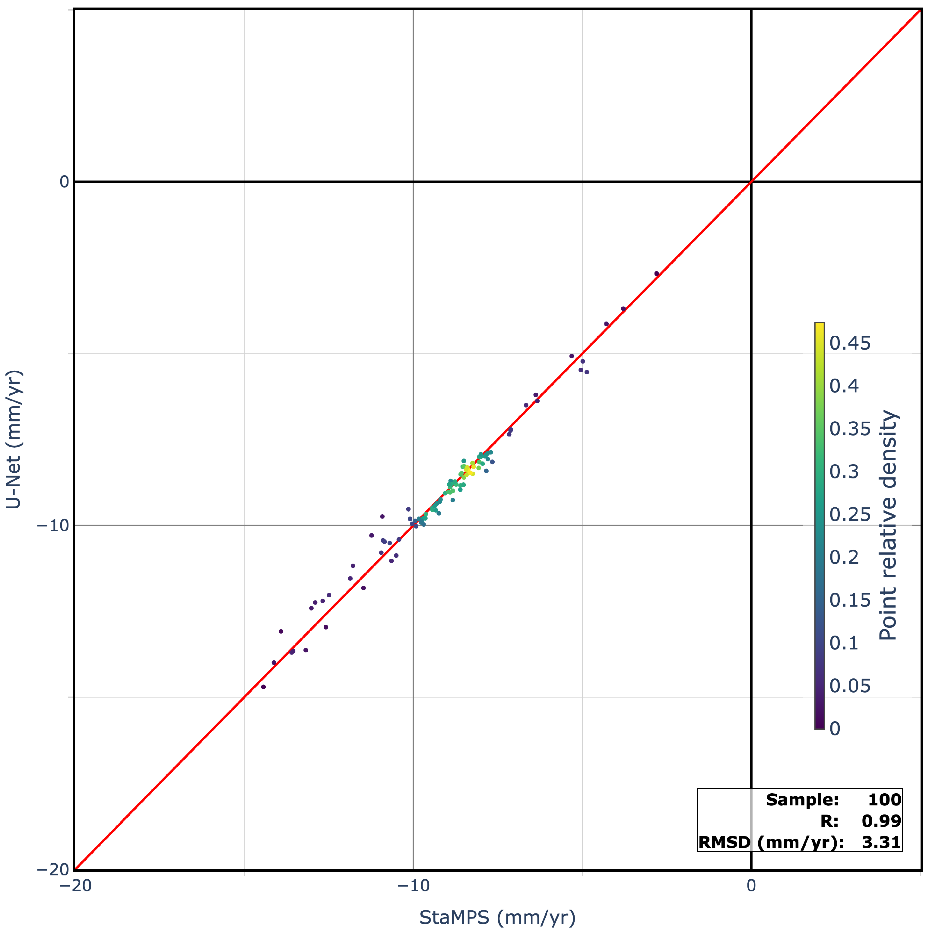
Consequently, the consistency of PSInSAR observations obtained from the conventional algorithm and the proposed neural network is evaluated. 100 PSs from the PSInSAR results are randomly selected and compared between the two approaches. For each selected PS, the mean LOS velocity within a 50-meter radius centered at that PS is computed and compared. The experimental results, illustrated in Figure 22, reveal a strong correlation between the LOS velocities derived from StaMPS-identified PSs and those predicted by the U-Net model, demonstrating the reliability of PSInSAR observations based on the suggested deep-learning approach.

In summary, this agreement indicates that the neural network-based iDS selection does not significantly compromise the derived deformation measurements despite the relatively low precision and F1-score observed in the classification results. This improvement holds particular promise for applications in non-urban or vegetated environments where conventional PS selection often suffers from sparse coverage and reduced reliability.

4.3. Application with a Limited Number of Interferograms

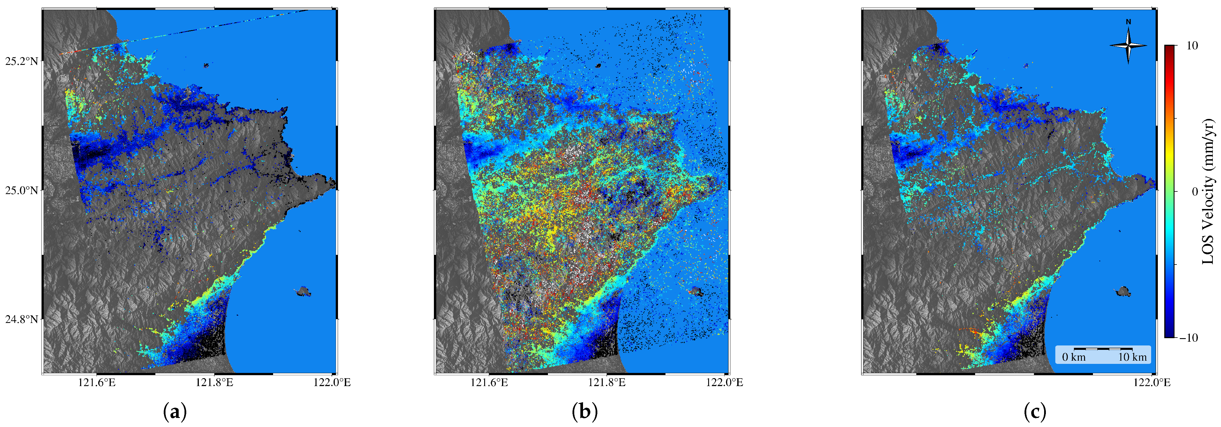
An additional advantage of this deep-learning-based method is the capability to estimate the iDS index from a single interferogram pair, enabling effective pixel classification even when only a small SAR image stack is available. As mentioned before, conventional PSInSAR processing typically requires at least 15 SAR images to ensure reliable PS identification and deformation estimation. In this section, an interferogram stack consisting of only 12 SAR images acquired between 12 January 2020 and 4 October 2022 is used as input to the neural network model to generate an iDS index, followed by phase processing to derive PSInSAR results. For comparison, the same data are applied to the StaMPS software to acquire another result that represents the measurement from the conventional algorithm. The LOS velocity, illustrated in Figure 23, demonstrates that the iDS distribution predicted by the deep-learning model closely resembles that obtained from the full StaMPS dataset, indicating robust iDS index estimation despite the reduced number of interferograms. In contrast, the conventional PSInSAR result derived from only 12 SAR images exhibits a degraded PS distribution, characterized by a substantial number of unreliable signals in low-coherence areas. These results highlight the advantage of the proposed approach in maintaining PS identification performance under data-limited conditions.

The results indicate that the proposed neural network model remains effective under limited SAR image availability, a condition commonly encountered when using high-resolution commercial satellite data, which are often characterized by restricted archives and high acquisition costs. Moreover, this approach enables timely deformation monitoring with high temporal resolution, whereas conventional PSInSAR algorithms typically require at least 15 SAR acquisitions to achieve comparable results.

5. Conclusions

With recent advances in computer technology and artificial intelligence, the application of deep learning techniques for the identification, classification, and exploitation of remote sensing imagery has become a rapidly developing research field. In this study, a U-Net-based neural network model, originally designed for medical image segmentation, was adapted to classify persistent scatterers in a radar interferogram. Benefiting from pixel-level recognition capability and modest training data requirements, supervised learning is successfully applied for iDS classification using Sentinel-1 data from central Taiwan and corresponding PSInSAR results. The trained model was subsequently applied to northern Taiwan and finally retrieved the spatial distribution of iDS pixels successfully. Validation shows that the model recovered approximately 92.81% of StaMPS-derived PSs, in terms of recall. In regions with low PS density, such as the large-scale landslide area investigated in northern Taiwan, the model identified additional iDSs beyond those detected by StaMPS, thereby enabling a more complete assessment of slope activity. Time-series analysis of these iDSs revealed deformation patterns in PS-deficient areas, demonstrating the potential of this approach to enhance InSAR monitoring in challenging environments.

Furthermore, the proposed method requires fewer interferograms for accurate iDS classification, allowing PSInSAR analysis to be performed with a limited number of SAR acquisitions. This characteristic highlights its suitability for operational applications using high-resolution commercial satellite imagery, where data availability is limited or acquisition costs are high.

References

1. Massonnet, D.; Feigl, K.L. Radar Interferometry and Its Application to Changes in the Earth’s Surface. Rev. Geophys. 1998, 36, 441–500. [Google Scholar] [CrossRef]
2. Ferretti, A.; Prati, C.; Rocca, F. Permanent Scatterers in SAR Interferometry. IEEE Trans. Geosci. Remote Sens. 2001, 39, 8–20. [Google Scholar] [CrossRef]
3. Hooper, A.; Zebker, H.; Segall, P.; Kampes, B. A New Method for Measuring Deformation on Volcanoes and Other Natural Terrains Using InSAR Persistent Scatterers. Geophys. Res. Lett. 2004, 31, L23611. [Google Scholar] [CrossRef]
4. Ferretti, A.; Fumagalli, A.; Novali, F.; Prati, C.; Rocca, F.; Rucci, A. A New Algorithm for Processing Interferometric Data-Stacks: SqueeSAR. IEEE Trans. Geosci. Remote Sens. 2011, 49, 3460–3470. [Google Scholar] [CrossRef]
5. Zhang, L.; Ding, X.; Lu, Z. Ground Settlement Monitoring Based on Temporarily Coherent Points between Two SAR Acquisitions. ISPRS J. Photogramm. Remote Sens. 2011, 66, 146–152. [Google Scholar] [CrossRef]
6. Sun, Q.; Zhang, L.; Ding, X.; Hu, J.; Liang, H. Investigation of Slow-Moving Landslides from ALOS/PALSAR Images with TCPInSAR: A Case Study of Oso, USA. Remote Sens. 2015, 7, 72–88. [Google Scholar] [CrossRef]
7. Mirzaee, S.; Motagh, M.; Akbari, B.; Wetzel, H.U.; Roessner, S. Evaluating three insar time-series methods to assess creep motion, Case study: Masouleh landslide in North Iran. ISPRS Ann. Photogramm. Remote Sens. Spat. Inf. Sci. 2017, IV-1-W1, 223–228. [Google Scholar] [CrossRef]
8. Zhang, B.; Wang, R.; Deng, Y.; Ma, P.; Lin, H.; Wang, J. Mapping the Yellow River Delta Land Subsidence with Multitemporal SAR Interferometry by Exploiting Both Persistent and Distributed Scatterers. ISPRS J. Photogramm. Remote Sens. 2019, 148, 157–173. [Google Scholar] [CrossRef]
9. Brengman, C.M.J.; Barnhart, W.D. Identification of Surface Deformation in InSAR Using Machine Learning. Geochem. Geophys. Geosyst. 2021, 22, e2020GC009204. [Google Scholar] [CrossRef]
10. Fiorentini, N.; Maboudi, M.; Leandri, P.; Losa, M.; Gerke, M. Surface Motion Prediction and Mapping for Road Infrastructures Management by PS-InSAR Measurements and Machine Learning Algorithms. Remote Sens. 2020, 12, 3976. [Google Scholar] [CrossRef]
11. Lattari, F.; Rucci, A.; Matteucci, M. A Deep Learning Approach for Change Points Detection in InSAR Time Series. IEEE Trans. Geosci. Remote Sens. 2022, 60, 1–16. [Google Scholar] [CrossRef]
12. Yin, W.; Chen, Q.; Feng, S.; Tao, T.; Huang, L.; Trusiak, M.; Asundi, A.; Zuo, C. Temporal Phase Unwrapping Using Deep Learning. Sci. Rep. 2019, 9, 20175. [Google Scholar] [CrossRef]
13. Zhang, L.; Huang, G.; Li, Y.; Yang, S.; Lu, L.; Huo, W. A Robust InSAR Phase Unwrapping Method via Improving the Pix2pix Network. Remote Sens. 2023, 15, 4885. [Google Scholar] [CrossRef]
14. Tiwari, A.; Narayan, A.B.; Dikshit, O. Deep Learning Networks for Selection of Measurement Pixels in Multi-Temporal SAR Interferometric Processing. ISPRS J. Photogramm. Remote Sens. 2020, 166, 169–182. [Google Scholar] [CrossRef]
15. Zhang, Y.; Wei, J.; Duan, M.; Kang, Y.; He, Q.; Wu, H.; Lu, Z. Coherent Pixel Selection Using a Dual-Channel 1-D CNN for Time Series InSAR Analysis. Int. J. Appl. Earth Obs. Geoinf. 2022, 112, 102927. [Google Scholar] [CrossRef]
16. Chen, S.; Zhao, C.; Jiang, M.; Yu, H. PSFNet: A Feature-Fusion Framework for Persistent Scatterer Selection in Multitemporal InSAR. IEEE J. Sel. Top. Appl. Earth Obs. Remote Sens. 2024, 17, 19972–19985. [Google Scholar] [CrossRef]
17. Hu, Z.; Li, M.; Li, G.; Wang, Y.; Sun, C.; Dong, Z. Persistent Scatterer Pixel Selection Method Based on Multi-Temporal Feature Extraction Network. Remote Sens. 2025, 17, 3319. [Google Scholar] [CrossRef]
18. Hung, W.C.; Hwang, C.; Chen, Y.A.; Chang, C.P.; Yen, J.Y.; Hooper, A.; Yang, C.Y. Surface Deformation from Persistent Scatterers SAR Interferometry and Fusion with Leveling Data: A Case Study over the Choushui River Alluvial Fan, Taiwan. Remote Sens. Environ. 2011, 115, 957–967. [Google Scholar] [CrossRef]
19. Chen, Y.A.; Chang, C.P.; Hung, W.C.; Yen, J.Y.; Lu, C.H.; Hwang, C. Space-Time Evolutions of Land Subsidence in the Choushui River Alluvial Fan (Taiwan) from Multiple-Sensor Observations. Remote Sens. 2021, 13, 2281. [Google Scholar] [CrossRef]
20. Colesanti, C.; Ferretti, A.; Prati, C.; Rocca, F. Monitoring Landslides and Tectonic Motions with the Permanent Scatterers Technique. Eng. Geol. 2003, 68, 3–14. [Google Scholar] [CrossRef]
21. Bovenga, F.; Wasowski, J.; Nitti, D.O.; Nutricato, R.; Chiaradia, M.T. Using COSMO/SkyMed X-band and ENVISAT C-band SAR Interferometry for Landslides Analysis. Remote Sens. Environ. 2012, 119, 272–285. [Google Scholar] [CrossRef]
22. Intrieri, E.; Raspini, F.; Fumagalli, A.; Lu, P.; Del Conte, S.; Farina, P.; Allievi, J.; Ferretti, A.; Casagli, N. The Maoxian Landslide as Seen from Space: Detecting Precursors of Failure with Sentinel-1 Data. Landslides 2018, 15, 123–133. [Google Scholar] [CrossRef]
23. Righini, G.; Pancioli, V.; Casagli, N. Updating Landslide Inventory Maps Using Persistent Scatterer Interferometry (PSI). Int. J. Remote Sens. 2012, 33, 2068–2096. [Google Scholar] [CrossRef]
24. Lu, C.Y.; Chan, Y.C.; Hu, J.C.; Tseng, C.H.; Liu, C.H.; Chang, C.H. Seasonal Surface Fluctuation of a Slow-Moving Landslide Detected by Multitemporal Interferometry (MTI) on the Huafan University Campus, Northern Taiwan. Remote Sens. 2021, 13, 4006. [Google Scholar] [CrossRef]
25. Krizhevsky, A.; Sutskever, I.; Hinton, G.E. ImageNet Classification with Deep Convolutional Neural Networks. Commun. ACM 2017, 60, 84–90. [Google Scholar] [CrossRef]
26. O’Shea, K.; Nash, R. An Introduction to Convolutional Neural Networks. arXiv 2015, arXiv:1511.08458. [Google Scholar] [CrossRef]
27. Long, J.; Shelhamer, E.; Darrell, T. Fully Convolutional Networks for Semantic Segmentation. In Proceedings of the IEEE Conference on Computer Vision and Pattern Recognition, Boston, MA, USA, 7–12 June 2015; pp. 3431–3440. [Google Scholar]
28. Ronneberger, O.; Fischer, P.; Brox, T. U-Net: Convolutional Networks for Biomedical Image Segmentation. In Proceedings of the Medical Image Computing and Computer-Assisted Intervention—MICCAI 2015; Navab, N., Hornegger, J., Wells, W.M., Frangi, A.F., Eds.; Springer: Munich, Germany, 2015; pp. 234–241. [Google Scholar] [CrossRef]
29. Hooper, A.; Segall, P.; Zebker, H. Persistent Scatterer Interferometric Synthetic Aperture Radar for Crustal Deformation Analysis, with Application to Volcán Alcedo, Galápagos. J. Geophys. Res. Solid Earth 2007, 112, 2006JB004763. [Google Scholar] [CrossRef]
30. Crosetto, M.; Monserrat, O.; Cuevas-González, M.; Devanthéry, N.; Crippa, B. Persistent Scatterer Interferometry: A Review. ISPRS J. Photogramm. Remote Sens. 2016, 115, 78–89. [Google Scholar] [CrossRef]
31. Abadi, M.; Agarwal, A.; Barham, P.; Brevdo, E.; Chen, Z.; Citro, C.; Corrado, G.S.; Davis, A.; Dean, J.; Devin, M.; et al. TensorFlow: Large-Scale Machine Learning on Heterogeneous Distributed Systems. arXiv 2016, arXiv:1603.04467. [Google Scholar] [CrossRef]
32. Kingma, D.P.; Ba, J. Adam: A Method for Stochastic Optimization. In Proceedings of the 3rd International Conference on Learning Representations, ICLR 2015, San Diego, CA, USA, 7–9 May 2015. [Google Scholar]
33. Bishop, C.M. Pattern Recognition and Machine Learning; Information Science and Statistics; Springer: New York, NY, USA, 2006. [Google Scholar]
34. Goodfellow, I.; Courville, A.; Bengio, Y. Deep Learning; Adaptive Computation and Machine Learning; The MIT Press: Cambridge, MA, USA, 2016. [Google Scholar]
35. Saito, T.; Rehmsmeier, M. The Precision-Recall Plot Is More Informative than the ROC Plot When Evaluating Binary Classifiers on Imbalanced Datasets. PLoS ONE 2015, 10, e0118432. [Google Scholar] [CrossRef]
36. He, H.; Garcia, E.A. Learning from Imbalanced Data. IEEE Trans. Knowl. Data Eng. 2009, 21, 1263–1284. [Google Scholar] [CrossRef]
37. Foody, G.M. Status of Land Cover Classification Accuracy Assessment. Remote Sens. Environ. 2002, 80, 185–201. [Google Scholar] [CrossRef]
38. Chang, L.; Hanssen, R.F. A Probabilistic Approach for InSAR Time-Series Postprocessing. IEEE Trans. Geosci. Remote Sens. 2016, 54, 421–430. [Google Scholar] [CrossRef]
39. Narayan, A.B.; Tiwari, A.; Dwivedi, R.; Dikshit, O. Persistent Scatter Identification and Look-Angle Error Estimation Using Similar Time-Series Interferometric Pixels. IEEE Geosci. Remote Sens. Lett. 2018, 15, 147–150. [Google Scholar] [CrossRef]
Figure 1. Area of interest used in this study: (a) An overview of Taiwan and the coverage. (b) The central Taiwan area used for model training.
Remotesensing 18 01181 g001
Figure 2. (a) An overview of the DInSAR dataset coverage, which is used to apply the deep-learning-based model for iDS prediction. (b) The optical image map of the large-scale landslide shows the distribution of vegetation coverage and structures in the study area.
Remotesensing 18 01181 g002
Figure 3. Data processing flow of deep learning iDS selection and PSInSAR processing, where “…” represents numerous samples omitted for brevity.
Remotesensing 18 01181 g003
Figure 4. Data processing flow of DInSAR and PSInSAR processing for the training dataset.
Remotesensing 18 01181 g004
Figure 5. The PS Index used in the model training step in this study.
Remotesensing 18 01181 g005
Figure 6. The architecture of the U-Net is proposed in this work.
Remotesensing 18 01181 g006
Figure 7. Illustration of binary classification results. (a) Sample distribution with actual class labels, where background regions indicate algorithm-derived ground truth boundaries (white: Positive; teal: Negative). (b) The same samples under model-predicted boundaries derived from the neural network. (c) Overlay of (a,b), illustrating the four classification outcomes: True Positive (TP), False Positive (FP), False Negative (FN), and True Negative (TN).
Remotesensing 18 01181 g007
Figure 8. Training and validation loss curves of the proposed U-Net model during the training process.
Remotesensing 18 01181 g008
Figure 9. The PS and iDS index applied to the interferogram in the urban area. The original interferogram and the wrap phase from the PS and iDS indices are listed in the columns. The optical and SAR intensity images are rendered in the last row.
Remotesensing 18 01181 g009
Figure 10. The PS and iDS index applied to the interferogram in the field area. The original interferogram and the wrap phase from the PS and iDS indices are listed in the columns. The optical and SAR intensity images are rendered in the last row.
Remotesensing 18 01181 g010
Figure 11. The line-of-sight velocity of PSInSAR produced by (a) the iDS index predicted by the U-Net model and (b) the PS index from StaMPS, while the white rectangle indicate the AOI of Figure 12.
Remotesensing 18 01181 g011
Figure 12. The PSInSAR result obtained by (a) iDS from the U-Net model and (b) PSs from StaMPS. The white circle indicated by letter A, B, C, D, E, and F are PS samples for time series analysis.
Remotesensing 18 01181 g012
Figure 13. The geometry between the satellite and the slope in this study indicates a shortening line-of-sight distance, representing an uplift velocity in the PSInSAR result.
Remotesensing 18 01181 g013
Figure 14. PS time series acquired from (a) U-Net at A, (b) StaMPS at A, (c) U-Net at B, (d) StaMPS at B, (e) U-Net at C, and (f) StaMPS at C.
Remotesensing 18 01181 g014
Figure 15. The phase ambiguity caused by excluding pixels with low coherence in the spatial domain could cause phase unwrapping error.
Remotesensing 18 01181 g015
Figure 16. iDS time series acquired from (a) U-Net at D, (b) U-Net at E, and (c) U-Net at F.
Remotesensing 18 01181 g016aRemotesensing 18 01181 g016b
Figure 17. The effect of the probability threshold on the evaluation metrics.
Remotesensing 18 01181 g017
Figure 18. The standard deviation of the line-of-sight velocity produced by (a) the iDS index predicted by the U-Net model and (b) the PS index from StaMPS.
Remotesensing 18 01181 g018
Figure 19. The distribution of LOS velocity standard deviation for (a) the PS and iDS. (b) The individual TP and FP from the iDS result.
Remotesensing 18 01181 g019
Figure 20. The histogram of ADI from (a) the PS and iDS. (b) The individual TP, FP, and FN ADI from the iDS result.
Remotesensing 18 01181 g020
Figure 21. The histogram of STIP from (a) the PS and iDS. (b) The individual TP, FP, and FN from the iDS result.
Remotesensing 18 01181 g021
Figure 22. The comparison of line-of-sight velocity from 100 random samples in the study area.
Remotesensing 18 01181 g022
Figure 23. (a) The LOS velocity of PSInSAR obtained using 12 SAR images with the iDS index predicted by the U-Net model and (b) the PS index from StaMPS. (c) The LOS velocity derives from corresponding 12 scene observations of the full dataset PSInSAR product.
Remotesensing 18 01181 g023