Application of the Fast Atmospheric Line-by-Line Code with Aerosol and Cloud Scattering (FALCAS) to TROPOMI Total Column Water Vapour Retrievals in the SWIR Band

Highlights

What are the main findings?

• FALCAS is developed as a fast line-by-line RT model with FOCAL-based scattering.
• FALCAS is applied to TROPOMI for TCWV retrievals, showing excellent agreement (correlation > 0.99) with the operational product.

What are the implications of the main findings?

• FALCAS enables accurate, efficient processing of hyperspectral satellite data.
• The approach has the potential for operational, large-scale TCWV retrievals.

Abstract

Fast radiative transfer models are essential for the efficient processing of hyperspectral satellite data in trace gas retrievals, as full multi-stream radiative transfer simulations are computationally demanding. We present FALCAS (Fast Atmospheric Line-by-line Code with Aerosol and Cloud Scattering), a surrogate forward model combining line-by-line radiative transfer with the virtual isotropic scattering layer approximation adopted from FOCAL. FALCAS retains much of the accuracy of full multi-stream calculations while enabling rapid simulations. Previously validated against synthetic spectra from a discrete ordinate radiative transfer model, FALCAS is here applied to real measurements from the TROPOspheric Monitoring Instrument (TROPOMI) to retrieve total column water vapour (TCWV) in the shortwave infrared band around 2.3 μm. Retrieval results are compared to the operational TROPOMI Level-2 TCWV from the CH₄ product. As this comparison is performed against an operational product from the same instrument, it represents an intercomparison rather than an evaluation against an independent reference dataset. FALCAS retrievals show a Pearson correlation coefficient greater than 0.99 with the operational data, and after empirical bias correction, the mean absolute bias across all regions is 1.45 mol m⁻² (0.12% relative) and the mean RMSE is 39.24 mol m⁻² (3.85% relative). These results demonstrate that FALCAS shows strong agreement with the operational TROPOMI Level-2 TCWV product, offering substantial computational advantages for large-scale processing.

1. Introduction

Water vapour is the dominant greenhouse gas and the primary gaseous source of infrared opacity in the atmosphere because it exhibits strong absorption features across a wide spectral range [1,2]. These pronounced and spectrally broad features significantly influence infrared radiative transfer and therefore must be accurately retrieved alongside other trace gases. The TROPOspheric Monitoring Instrument (TROPOMI), on board the Sentinel-5 Precursor satellite, provides global coverage of total column water vapour (TCWV) measurements in the shortwave infrared (SWIR) spectral range, with high spatial resolution and a daily revisit time [3]. TCWV serves as an important parameter for the retrieval of CH₄ in the SWIR band, and accurate knowledge of TCWV is essential for improving the reliability of CH₄ retrievals.

Retrieval algorithms for TROPOMI typically rely on radiative transfer (RT) models that solve the radiative transfer equation (RTE), with multiple scattering explicitly taken into account [4,5,6]. Such multi-stream models offer high physical accuracy but are computationally demanding, particularly at high spectral resolution and when applied to large datasets. This computational burden poses challenges for near-real-time applications and for the reprocessing of multi-year global archives at full resolution. Several approximations have been proposed to accelerate the solution of RTE, including the small-angle modification of the discrete ordinate method [7,8] and approaches based on asymptotic theory [9]. A comprehensive review of these methods is provided in [10].

Another important challenge arises from the large number of spectral points in the SWIR range required for TCWV retrievals, which makes hyperspectral RT simulations particularly time-consuming.

Several approaches have been developed to accelerate such computations. For instance, the correlated-k method [11,12,13] speeds up radiative transfer calculations by computing radiances at selected wavelengths and then using the statistical distribution of radiative properties to approximate values at the other wavelengths. Another approach is to perform low-stream radiative transfer simulations at all spectral points and then apply correction techniques to approximate multi-stream accuracy. In principal component analysis (PCA) [14,15], the full low-stream spectra are projected onto a small set of principal components, and a few multi-stream calculations are used to reconstruct the high-accuracy full-spectrum radiances. Similarly, the Cluster Low-Streams Regression (CLSR) method [16,17] uses the low-stream radiances to form clusters of similar values, computes multi-stream radiances for a few representative points in each cluster, and then applies a regression to predict accurate radiances across the spectrum. Nevertheless, these methods accelerate computations within the framework of conventional radiative transfer solvers. In such models, multiple scattering is still treated numerically, so the fundamental complexity of the scattering problem remains unchanged.

Recent studies have explored data-driven approaches that directly approximate the inverse mapping from measured spectra to geophysical parameters. For example, physics-constrained Bayesian neural networks have been applied to hyperspectral satellite measurements to retrieve aerosol properties with accuracy comparable to operational products, while achieving substantial reductions in computational cost and providing explicit uncertainty quantification [18,19]. However, such approaches rely on representative training datasets and may exhibit reduced generalisation capability when applied to atmospheric conditions or observational geometries that are not well represented in the training data. This highlights the continued relevance of physically based methods that do not require prior training and remain robust across a wide range of conditions.

A promising alternative is the use of surrogate RT forward models that approximate the effect of multiple scattering within a simplified but tunable framework [20]. This approach can substantially reduce the computational requirements of hyperspectral simulations while retaining much of the accuracy of full multi-stream calculations. One example of such a surrogate RT model is the FOCAL (Fast atmOspheric traCe gAs Retrieval) model [21,22], in which the scattering process is represented by an optically thin, isotropic scattering layer. This approximation emulates the isotropisation effect of multiple scattering while avoiding the computational cost associated with explicitly solving the full multi-stream RTE. By modelling scattering in this simplified yet physically motivated manner, FOCAL substantially reduces computational load, enabling faster trace gas retrievals from hyperspectral measurements. In the original studies, the FOCAL model was applied to the retrieval of XCO₂ from Orbiting Carbon Observatory-2 measurements, demonstrating its ability to achieve high retrieval accuracy at a fraction of the computational cost of traditional RT approaches.

In our previous work [23], we introduced the Fast Atmospheric Line-by-line Code with Aerosol and Cloud Scattering (FALCAS), a surrogate RT model that replaces explicit multiple scattering calculations with an effective isotropisation treatment via a single, optically thin scattering layer. The multiple scattering concept is adopted from FOCAL, while the model itself is independently implemented using the Py4CAtS line-by-line modules [24,25]. The model includes tunable parameters that can be optimised during the retrieval to match a reference spectrum, thereby compensating for the simplifications in the scattering treatment. We demonstrated the accuracy of FALCAS using synthetic spectra generated with the multi-stream discrete ordinate model PYDOME [26,27] as a reference, showing that CH₄ retrieval errors remained within 2% under typical atmospheric conditions.

In this study, we extend the application of FALCAS to real TROPOMI measurements for TCWV retrieval in the 2305–2345 nm spectral range. The main goal is to investigate the accuracy and robustness of the FALCAS model when applied to TCWV retrievals from hyperspectral satellite observations. We compare the results with the official TROPOMI Level 2 TCWV from the CH₄ product. In addition to assessing the overall agreement, we analyse how retrieval accuracy depends on key observational and geophysical parameters, including solar and viewing geometry, surface albedo, and aerosol loading. This evaluation allows us to assess whether the computational advantages of FALCAS can be realised for large-scale TCWV monitoring while maintaining strong consistency with the operational TROPOMI product.

2. Materials and Methods

2.1. Forward Model FALCAS

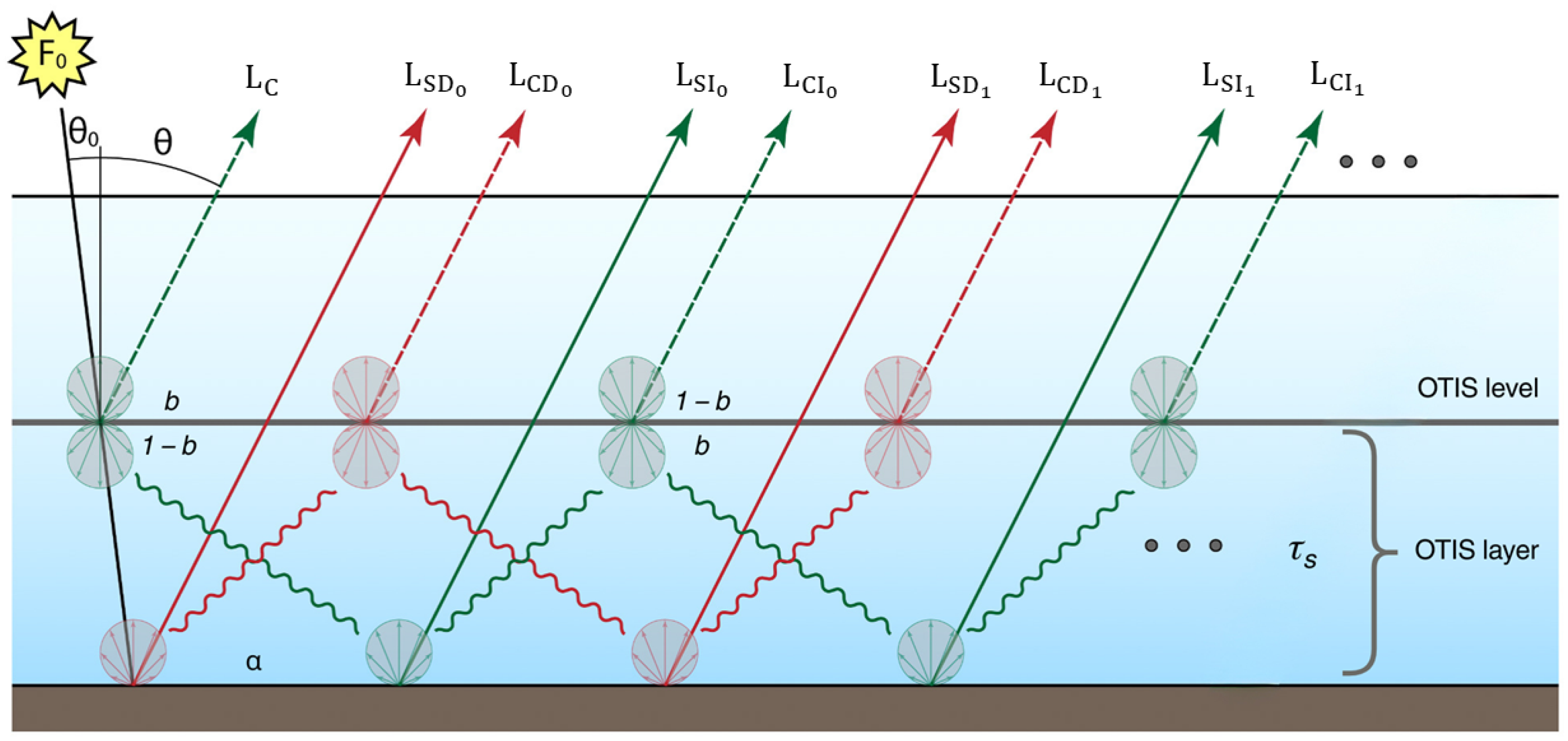
FALCAS is a Python-based forward model under development at DLR, designed for the efficient simulation of solar radiation measurements in trace gas retrievals. The key idea is to represent multiple scattering through an optically thin isotropic scattering (OTIS) level [21], rather than by solving the full multi-stream radiative transfer equation. The OTIS level (Figure 1) is an infinitesimal geometric plane at which scattering is isotropic, while the OTIS layer refers to the atmosphere below this level. Consistent with the definition of optical thickness as increasing downward from the top of the atmosphere, the cumulative scattering optical thickness of the OTIS layer is effectively represented at the OTIS level. At the OTIS level, light is isotropically transmitted in either the forward or backward direction based on the back-scattering fraction. The concept was first implemented in the FOCAL model [21,22] and is here realised independently using the Py4CAtS line-by-line modules [24].

The isotropic scattering at the OTIS level generates an infinite number of light paths reaching the satellite. For instance, the surface-direct component $L_{SD}$ is the sum of individual contributions $L_{S{D}_i}$, i.e., $L_{S{D}_0} ,L_{S{D}_1} ,L_{S{D}_2},\dots$. The infinite sum of reflections between the OTIS level and the surface is approximated by

$$\rho \approx {\displaystyle \frac{1}{1-\alpha S_F({\tau }_s,{\tau }_e,{\tau }_{\downarrow })b{\left(T_F^g\left({\tau }_{\downarrow }\right)\right)}^2}},$$

(1)

where $\rho$ is the diffuse reflectance, $\alpha$ the surface albedo, b the back-scattering fraction, ${\tau }_s$ the scattering optical thickness, ${\tau }_e$ the extinction optical thickness, and ${\tau }_{\downarrow }$ the gaseous optical thickness below the OTIS level. The transmission and scattering terms are

$$T_F^g\left({\tau }_{\downarrow }\right)=2E_3\left({\tau }_{\downarrow }\right),S_F({\tau }_s,{\tau }_e,{\tau }_{\downarrow })={\displaystyle \frac{{\tau }_s}{{\tau }_e}}\left[1-{\displaystyle \frac{E_3({\tau }_{\downarrow }+{\tau }_e)}{E_3\left({\tau }_{\downarrow }\right)}}\right],$$

(2)

where $E_n\left(\tau \right)={\int }_1^{\infty }{e}^{-\tau s}{s}^{-n}ds$ is the generalised exponential integral.

The radiance at the top of atmosphere (TOA) is expressed as

$$L=L_C+L_{SD}+L_{CD}+L_{SI}+L_{CI},$$

(3)

where $L_C$ is the radiance directly scattered from the OTIS level, $L_{SD}$ is the radiance from the surface due to direct illumination, $L_{CD}$ is the radiance from the OTIS level due to direct illumination of the surface, $L_{SI}$ is the radiance from the surface due to diffuse illumination from the OTIS level, and $L_{CI}$ is the radiance from the OTIS level due to diffuse illumination.

The five components in Equation (3) are:

$$\begin{array}{cc}\hfill L_C& =L_0{S}_I({\tau }_s,{\tau }_e,{\zeta }_0)b,\hfill \end{array}$$

(4)

$$\begin{array}{cc}\hfill L_{SD}& =L_0\alpha T_I^s({\tau }_e,{\zeta }_0)T_I^s({\tau }_e,\zeta )T_I^g({\tau }_{\downarrow },{\zeta }_0)T_I^g({\tau }_{\downarrow },\zeta )\rho ,\hfill \end{array}$$

(5)

$$\begin{array}{cc}\hfill L_{CD}& =L_0\alpha T_I^s({\tau }_e,{\zeta }_0)S_F({\tau }_s,{\tau }_e,{\tau }_{\downarrow })f{T}_I^g({\tau }_{\downarrow },{\zeta }_0)T_F^g\left({\tau }_{\downarrow }\right)\rho ,\hfill \end{array}$$

(6)

$$\begin{array}{cc}\hfill L_{SI}& =L_0\alpha S_I({\tau }_s,{\tau }_e,{\zeta }_0)f{T}_I^s({\tau }_e,\zeta )T_F^g\left({\tau }_{\downarrow }\right)T_I^g({\tau }_{\downarrow },\zeta )\rho ,\hfill \end{array}$$

(7)

$$\begin{array}{cc}\hfill L_{CI}& =L_0\alpha S_I({\tau }_s,{\tau }_e,{\zeta }_0)S_F({\tau }_s,{\tau }_e,{\tau }_{\downarrow })f^2{\left[T_F^g\left({\tau }_{\downarrow }\right)\right]}^2\rho ,\hfill \end{array}$$

(8)

with

$$L_0={\displaystyle \frac{F_0}{\pi {\zeta }_0}}{T}_I^g({\tau }_{\uparrow },{\zeta }_0+\zeta ),S_I({\tau }_s,{\tau }_e,{\zeta }_0)={\displaystyle \frac{{\tau }_s}{{\tau }_e}}\left[1-e^{-{\tau }_e{\zeta }_0}\right],$$

(9)

where $F_0$ is the solar irradiance, ${\zeta }_0=1/cos{\theta }_0$ and $\zeta =1/cos\theta$ are the slant path factors for the Sun and satellite, ${\tau }_{\downarrow }$ and ${\tau }_{\uparrow }$ are gaseous optical thicknesses below and above the OTIS level, $T_I^s$ and $T_I^g$ are transmission terms, $S_I$ and $S_F$ are scattering terms, and $f=1-b$. These transmission terms are explicitly given by

$$T_I^s(\tau ,\zeta )=e^{-\tau \zeta },T_I^g(\tau ,\zeta )=e^{-\tau \zeta },$$

(10)

where the appropriate optical thickness and slant path factors (e.g., ${\tau }_{\downarrow }$, ${\zeta }_0$) are inserted for each term in Equations (4)–(8). The forward simulation of a spectrum using FALCAS takes less than 0.1 s, given that the absorption coefficients are pre-computed. For comparison, a full line-by-line simulation using PYDOME requires approximately 400 s for the same spectrum.

2.2. Inversion Algorithm

The total column water vapour (TCWV) retrieval from TROPOMI shortwave infrared measurements using FALCAS is formulated as a nonlinear least-squares problem. The objective function quantifies the difference between simulated and measured top-of-atmosphere (TOA) radiances.

First, the FALCAS forward model is run at high spectral resolution (79,002 spectral points in the 2305–2345 nm window), producing $I_{\mathrm{FALCAS},\mathrm{HR}}(\lambda ;\mathit{\theta })$, where $\lambda$ denotes the spectral samples and $\mathit{\theta }$ is the state vector. The nine parameters of $\mathit{\theta }$ are listed in

Table 1. State vector parameters used in the TCWV retrieval.

Parameter	Description
TCWV	Total column water vapour
XCH4	Dry-air mole fraction of methane
Ground albedo	Surface reflectance at reference wavelength
Albedo slope (1st order)	Linear spectral dependence of surface albedo
Albedo curvature (2nd order)	Quadratic spectral dependence of surface albedo
Back-scattering fraction	Fraction of back-scattering at OTIS level
OTIS layer height	Effective altitude of isotropic scattering layer
Ångström turbidity	Amplitude of aerosol optical thickness (AOT)
Ångström exponent	Spectral slope of AOT

.

The aerosol optical thickness (AOT) at any wavelength $\lambda$ can be calculated from the retrieved Ångström parameters as

$$\mathrm{AOT}\left(\lambda \right)=\AA ngström\mathrm{turbidity}·{\lambda }^{-\AA ngström\mathrm{exponent}}.$$

(11)

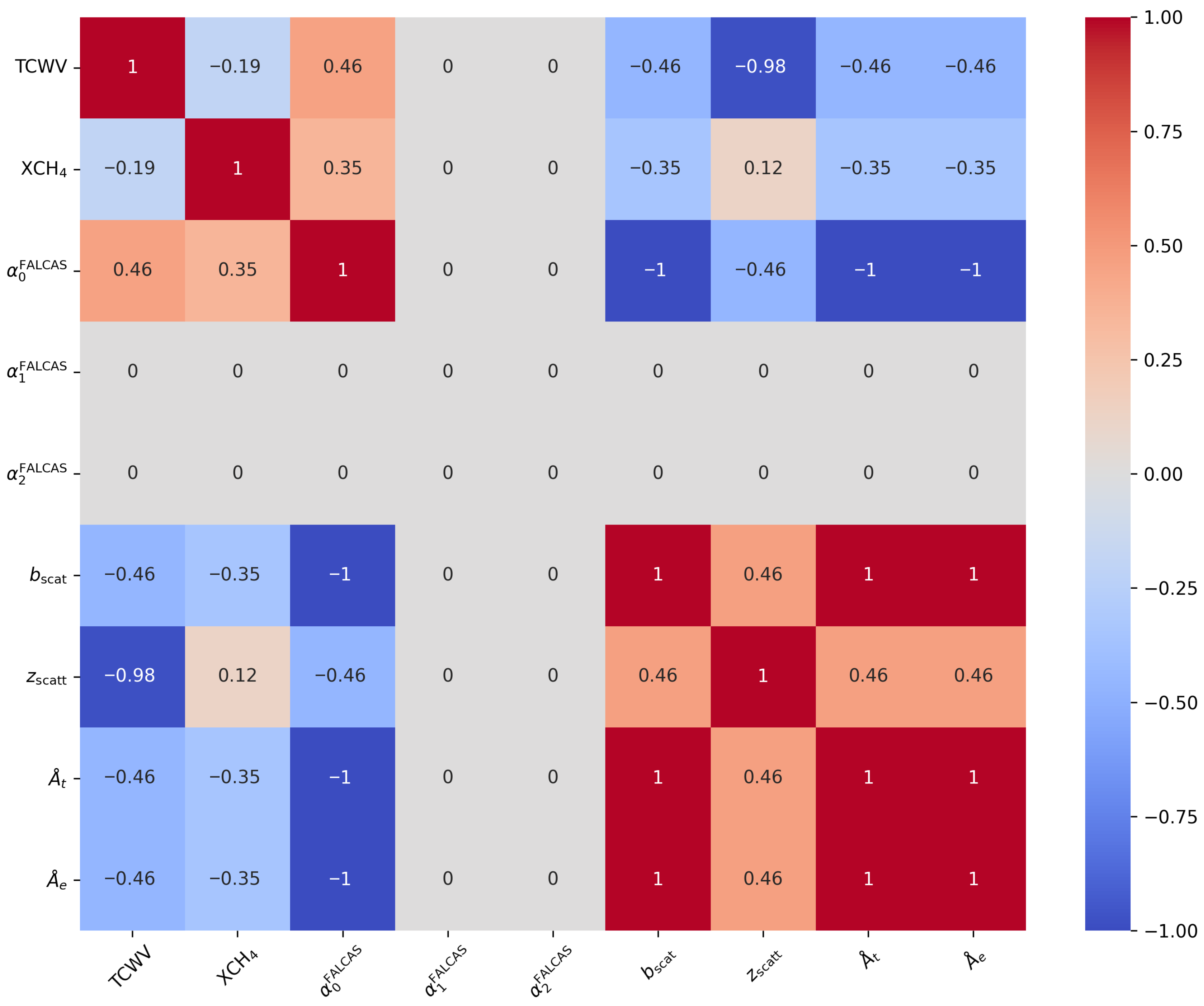
To assess potential compensation effects and the constraints of the fitted state vector parameters, we computed the correlation matrix of radiance derivatives with respect to the nine parameters (Figure 2). Each derivative was calculated using a finite-difference approach by individually perturbing one parameter while keeping the others fixed. The resulting correlation matrix quantified potential compensation between parameters, where values close to $\pm 1$ indicated strong correlation and values near 0 indicated weak correlation.

We observed that TCWV exhibited a strong negative correlation with the OTIS layer height. Both retrieval versions, with and without optimising the OTIS layer height, were tested, and including this parameter yielded improved results on our test cases. Therefore, the OTIS layer height was retained in the retrieval. Other parameters, including ground albedo, albedo slope, albedo curvature, back-scattering fraction, Ångström turbidity, and Ångström exponent, occasionally showed high correlations in certain spectral regions or scenarios. This behaviour has been previously addressed using synthetic data, and given our primary focus on water vapour retrieval, we consider this acceptable for the current study. We note that the derivatives of albedo slope and albedo curvature are extremely small, resulting in near-zero values in the correlation matrix. Nonetheless, these parameters were included in the retrieval since the official TROPOMI product also considers them.

The high-resolution spectrum is then convolved with the TROPOMI slit function $S\left(\lambda \right)$, which has a full width at half maximum (FWHM) of 0.32–0.34 nm, yielding the instrument-resolution spectrum:

$$I_{\mathrm{FALCAS}}\left(\lambda \right)=\int I_{\mathrm{FALCAS},\mathrm{HR}}\left({\lambda }^{\prime }\right)S(\lambda -{\lambda }^{\prime })d{\lambda }^{\prime }.$$

(12)

The cost function to be minimised is defined as

$$J\left(\mathit{\theta }\right)=\sum _{\lambda }{\left[I_{\mathrm{FALCAS}}(\lambda ;\mathit{\theta })-I_{\mathrm{meas}}\left(\lambda \right)\right]}^2,$$

(13)

where $I_{\mathrm{meas}}\left(\lambda \right)$ is the measured TOA radiance.

Minimisation of $J\left(\mathit{\theta }\right)$ is performed using the quasi-Newton Broyden–Fletcher–Goldfarb–Shanno (BFGS) algorithm [28]. The workflow follows these steps [23]:

• Initialisation: Parameters are normalised to comparable magnitudes; initial guesses are drawn from uniform distributions over physically plausible ranges.
• Multistart strategy: The inversion is repeated for $N_{\mathrm{start}}=10$ random initialisations. The solution with the smallest residual is selected.
• Gradient evaluation: Jacobians are computed via finite differences, with step sizes tuned to balance stability and accuracy.
• Convergence criteria: Iterations terminate when the relative change in the objective function or gradient norm falls below ${10}^{-5}$.
• Parallelisation: Multistart runs are distributed across available CPU cores, reducing wall-clock time by ~90%.

This approach is computationally efficient: for a single TROPOMI pixel, the full retrieval, including all multistart fits, takes approximately 29 s using 30 parallel workers on an Intel Xeon Platinum 8380 processor. In our previous synthetic study [23], the multistart strategy substantially improved robustness, avoiding suboptimal convergence in over 80% of cases under conditions of high aerosol loading or low signal-to-noise ratio (SNR).

2.3. Retrieval Process

The retrieval workflow applied in this study consists of three components: pre-processing, processing, and post-processing with error analysis. In the pre-processing stage, TROPOMI Level-1B radiance data—the input to our retrieval—are selected based on the target region and time period, and filtered for quality. The processing stage includes convolution of the input spectra with the instrument spectral response function (ISRF) to ensure consistency with the FALCAS forward model, followed by retrieval using a quasi-Newton BFGS algorithm with a multistart strategy. Post-processing is applied to correct systematic biases in the retrieved TCWV values. This bias correction enables a robust error analysis to quantify the influence of auxiliary parameters on the agreement with the operational TROPOMI product.

2.3.1. Pre-Processing

TROPOMI measurements are used to evaluate the retrieval accuracy of FALCAS for real atmospheric data. Level-1B Band 7 radiance and SWIR irradiance products provide spectra covering 2305–2345 nm at 0.227 nm resolution. TROPOMI Level-2 TCWV from the CH₄ product is employed for comparison. Thirteen regions covering major continents and oceans are investigated. For each region, one NetCDF file from June to August 2021 containing the largest number of valid TCWV measurements is selected.

Spectral channel quality, ground pixel quality, and TCWV QA values are used for filtering. The spectra with fewer than four defective channels, QA above 80, solar zenith angle (SZA) and viewing zenith angle (VZA) below 70°, and cloud fraction below 0.1 are retained. After filtering, 58,625 valid retrieval points remain across all considered regions, corresponding to approximately 33% of the initially available observations. The regional distribution of the retained samples is as follows: Australia (11,580), Central Asia (7918), China (1728), eastern Atlantic Ocean (973), eastern North America (2644), eastern South America (4047), Europe (3180), North Africa (3578), Pacific Ocean (693), South Africa (10,901), western Atlantic Ocean (1035), western North America (4802), and western South America (5546).

2.3.2. Processing

High-resolution FALCAS spectra are convolved with the instrument spectral response function (ISRF) from the TROPOMI calibration database [29] to match the instrument resolution. The ISRF kernel is defined on 480 wavelength steps, with each pixel represented by 1025 values, and is interpolated to all TROPOMI spectral points. The FALCAS grid is converted from wavenumber to wavelength space, with 79,002 spectral points used to match the ISRF resolution of 0.0009765625 nm.

Reference atmospheric profiles are adapted using temperature, humidity, surface pressure, and cloud fraction from ECMWF. SZA and VZA are fixed, while the other state vector parameters (Table 1) are retrieved. Although spectra with four or more defective channels are excluded during pre-processing, the remaining spectra may still contain up to three defective channels; these channels are omitted from the retrieval calculation. TCWV is then retrieved using the quasi-Newton BFGS inversion algorithm with a multistart strategy (see Section 2.2).

2.3.3. Post-Processing and Error Analysis

Before applying any post hoc adjustments, the raw TCWV-FALCAS retrievals are evaluated by comparison with the operational TROPOMI measurements. This comparison represents the intrinsic performance of the FALCAS forward model without any external correction. For both the raw and post-corrected datasets, model performance is quantified using bias and relative bias (%), root-mean-square error (RMSE) and relative RMSE (%), as well as the Pearson correlation coefficient (r).

Empirical bias correction is applied to the retrieved TCWV values using linear regression with TROPOMI measurements. For each region, the collocated dataset is divided into independent training and test subsets using a 70%/30% split. The resulting sample sizes for the training and test subsets are as follows: Australia (8105/3475), Central Asia (5542/2376), China (1209/519), eastern Atlantic Ocean (681/292), eastern North America (1850/794), eastern South America (2832/1215), Europe (2226/954), North Africa (2504/1074), Pacific Ocean (485/208), South Africa (7630/3271), western Atlantic Ocean (724/311), western North America (3361/1441), and western South America (3882/1664), where the numbers correspond to training and test samples, respectively. The correction model is fitted exclusively on the training subset and subsequently evaluated on the independent test subset. This ensures that the reported metrics are out-of-sample and not artificially optimistic. The purpose of this bias correction is not to enhance the retrieval model itself, but to reduce systematic offsets in order to establish a consistent baseline for subsequent analysis of retrieval errors. In particular, by minimising systematic bias, the influence of auxiliary parameters on retrieval accuracy can be more clearly identified.

Auxiliary parameters potentially affecting retrieval accuracy are analysed using a random forest classification model [30]. Relative differences between FALCAS and TROPOMI TCWV are computed for all samples, and the 15% of observations with the largest differences are labelled as “low-correlation,” while the remaining 85% are labelled as “high-correlation.” The 15% threshold was chosen based on an analysis of the distribution of relative differences between FALCAS and TROPOMI TCWV for each region. The differences are generally centred near zero, indicating good retrieval performance, but a small fraction of points exhibit larger deviations. By examining these distributions, we selected 15% to focus on the most extreme deviations while retaining sufficient samples for robust classification.

The dataset is split into training and test subsets with a test size of 20%. Random forest classifiers with 20 trees and balanced class weights are trained to identify the parameters most strongly associated with low-correlation cases. Rather than focusing on classification performance, the analysis emphasises feature importance to determine which auxiliary parameters contribute most significantly to retrieval errors. In the following sections, this approach is referred to as the regional correlation classification model.

The included auxiliary parameters are: SZA, VZA, surface elevation, surface albedo (from TROPOMI and optimised FALCAS), aerosol optical thickness (SWIR and NIR), FALCAS Ångström turbidity coefficient and exponent, number of defective channels, and radiance/irradiance signal-to-noise ratio (SNR) and spectral error ratio (SER). Surface elevation is derived from ETOPO 2022 [31] and interpolated to the measurement locations.

3. Results

TCWV is retrieved from TROPOMI Level-1B data using the FALCAS forward model in combination with a quasi-Newton BFGS inversion algorithm with a multistart strategy. The TCWV retrieved using FALCAS is referred to as TCWV-FALCAS, while the operational TROPOMI Level-2 TCWV product, derived from the CH₄ retrieval, is referred to as TCWV-TROPOMI.

In this section, TCWV-FALCAS is compared with TCWV-TROPOMI for each region to assess agreement. Subsequently, an empirical bias correction is applied to TCWV-FALCAS to reduce systematic differences relative to TROPOMI. Finally, auxiliary parameters that may influence the retrieval results are analysed using a regional correlation classification model based on a random forest machine-learning approach.

3.1. Raw Comparison to Operational TROPOMI TCWV

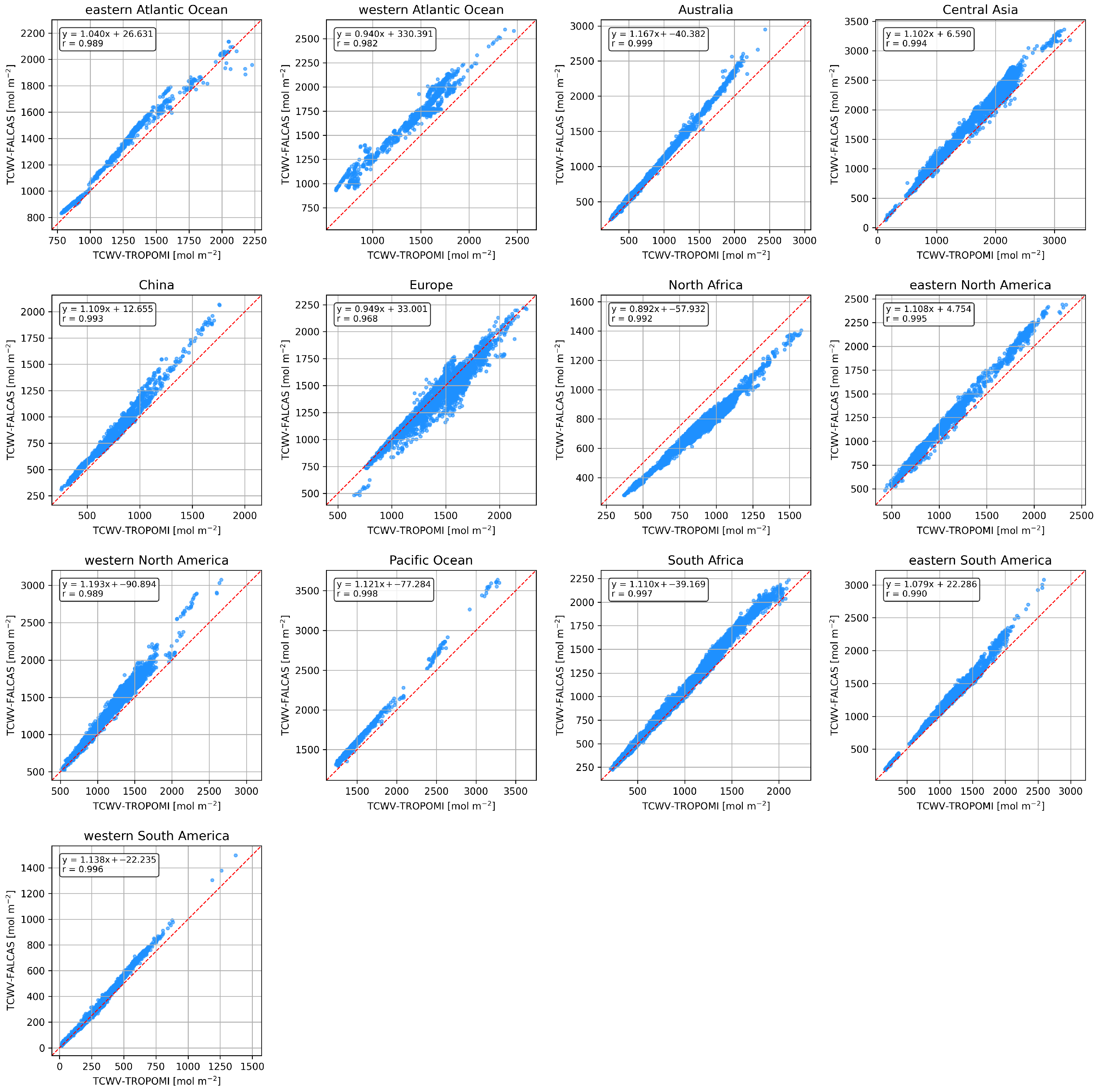
First, we assess the uncorrected agreement between TCWV-FALCAS and TCWV-TROPOMI for the selected regions. Figure 3 presents this comparison, with TCWV-FALCAS showing good overall agreement with TCWV-TROPOMI over both land and ocean, as reflected in high correlation coefficient values (0.99). However, in most regions—including Australia, China, eastern North America, western North America, the Pacific Ocean, eastern South America, and western South America—the regression slopes exceed unity, indicating a systematic overestimation of TCWV-FALCAS relative to TCWV-TROPOMI at high TCWV values. In addition, the variability in slopes and offsets across regions suggests that a single global correction may not perform equally well under all regional conditions.

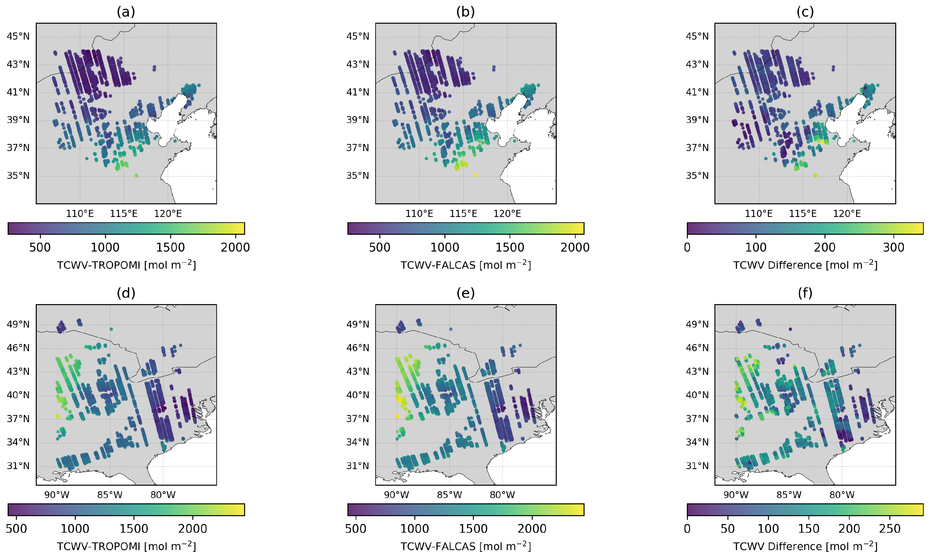
To illustrate how a correlation slope exceeding unity appears in the spatial distribution of TCWV, two regions—China and eastern North America—are selected as examples. Figure 4 shows the spatial distribution of TCWV over these regions: (a) TROPOMI over China, (b) FALCAS over China, (c) absolute TCWV difference between FALCAS and TROPOMI over China, (d) TROPOMI over eastern North America, (e) FALCAS over eastern North America, and (f) absolute TCWV difference between FALCAS and TROPOMI over eastern North America. TCWV-FALCAS and TCWV-TROPOMI are in close agreement when TCWV values are below 1500 mol m⁻². However, for TCWV values exceeding 1500 mol m⁻², TCWV-FALCAS tends to overestimate relative to TCWV-TROPOMI.

3.2. Empirical Bias Correction Relative to TROPOMI

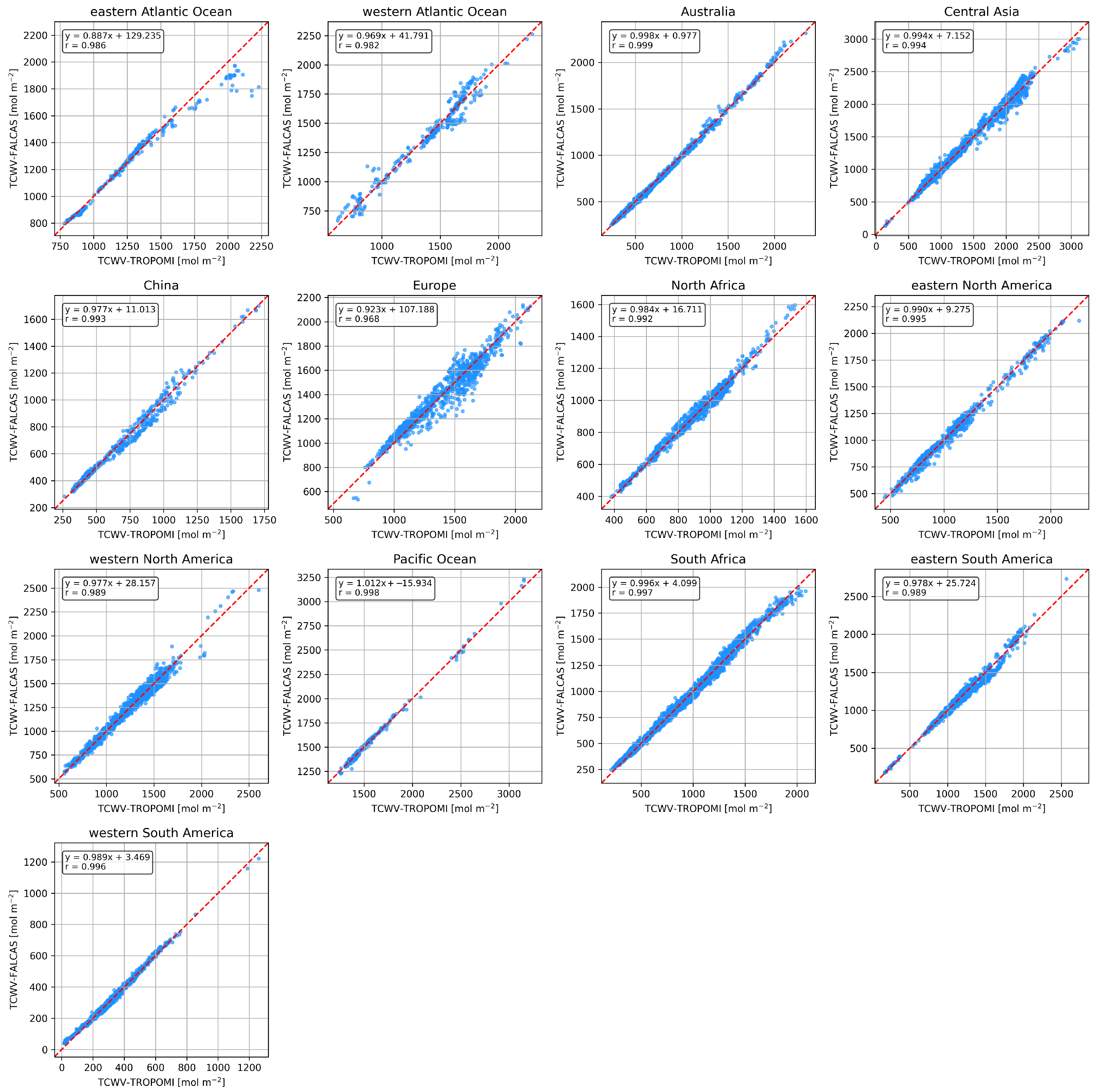
Second, an empirical bias correction relative to TROPOMI is applied to reduce systematic deviations between TCWV-FALCAS and TCWV-TROPOMI (for details, see Section 2.3.3). Figure 5 presents the correlation plots of TCWV-FALCAS and TCWV-TROPOMI after bias correction, evaluated on the 30% independent test dataset. The purpose of this regional empirical bias correction is not to generate a correction model for operational use, but to reduce systematic deviations and establish a consistent baseline for accurately analysing FALCAS performance in the following sections. Due to the region-specific differences in slopes and offsets observed in the raw data, a single global correction model cannot be reliably applied across all regions. Compared to Figure 4, most regions show a significant improvement in the linear regression fit, with slopes and offsets closer to the 1:1 relationship. However, in the eastern Atlantic Ocean, outlier values appear where TCWV-TROPOMI exceeds 2000 mol m⁻², and in Europe, a convex-like distortion is observed around the middle of the diagonal.

Table 2. Statistical comparison between TCWV-FALCAS and TCWV-TROPOMI over different regions for raw and bias-corrected test datasets. For each cell, the first value represents the absolute quantity in mol m⁻², and the value in parentheses is the relative quantity in %. The last row shows the mean across all regions.

Region	Raw Data		Bias-Corrected Data		r
	Bias	RMSE	Bias	RMSE
Eastern Atlantic	76.0 (6.2)	87.9 (7.2)	−12.33 (−0.97)	62.62 (4.92)	0.986
Western Atlantic	246.1 (17.4)	254.7 (18.0)	−4.50 (−0.32)	61.52 (4.37)	0.984
Australia	48.5 (9.1)	73.7 (13.8)	−0.12 (−0.02)	15.81 (2.97)	0.999
Central Asia	130.0 (10.7)	149.1 (12.3)	−1.86 (−0.15)	49.35 (4.08)	0.994
China	84.4 (12.8)	97.9 (14.9)	−0.39 (−0.06)	35.04 (5.37)	0.992
Europe	−38.0 (−2.7)	82.0 (5.9)	−0.24 (−0.02)	70.89 (5.11)	0.969
North Africa	−157.8 (−17.0)	161.0 (17.4)	0.73 (0.08)	25.76 (2.78)	0.992
Eastern N. America	123.6 (11.3)	134.9 (12.3)	−1.60 (−0.15)	34.14 (3.12)	0.995
Western N. America	143.1 (11.8)	163.2 (13.5)	2.15 (0.18)	44.02 (3.63)	0.989
Pacific Ocean	117.6 (7.3)	129.2 (8.0)	−0.69 (−0.04)	22.87 (1.43)	0.998
South Africa	43.8 (5.8)	67.8 (9.0)	0.53 (0.07)	27.00 (3.57)	0.998
Eastern S. America	115.9 (9.8)	128.8 (10.9)	−0.61 (−0.05)	46.91 (3.95)	0.989
Western S. America	22.1 (6.9)	31.6 (9.8)	−0.51 (−0.16)	12.17 (3.77)	0.996
Mean (all regions)	91.3 (8.8)	118.2 (10.7)	−1.45 (−0.12)	39.24 (3.85)	0.991

summarises the statistical comparison between TCWV-FALCAS and TCWV-TROPOMI across the different regions for both the raw and bias-corrected test datasets. Overall, the bias correction substantially reduces systematic deviations: the mean absolute bias across all regions decreases from 91.3 mol m⁻² (8.8%) to 1.45 mol m⁻² (0.12%), and the mean RMSE decreases from 118.2 mol m⁻² (10.7%) to 39.24 mol m⁻² (3.85%).

Region-specific differences are also evident. In the eastern Atlantic Ocean, the bias after correction remains relatively high (−12.33 mol m⁻², −0.97%) compared to other regions, which reflects the presence of outlier values in the correlation plots at high TCWV-TROPOMI (>2000 mol m⁻²). In Europe, the Pearson correlation coefficient after correction (0.969) is lower than in most other regions, consistent with the convex-like distortion observed around the middle of the diagonal in the corresponding correlation subplot.

These observations indicate that, while the bias correction is generally effective in the selected regions, region-specific features and extreme values can still influence the retrieval errors. To investigate the origin of these remaining discrepancies, potential auxiliary parameters are analysed using a regional correlation classification model constructed with a random forest machine-learning method.

3.3. Analysis of Post-Correction Retrieval Error

Third, we analyse retrieval errors after correction to identify remaining scene-dependent effects. Regional correlation classification models are developed using a random forest machine-learning approach to investigate the factors influencing deviations between TCWV-FALCAS and TCWV-TROPOMI.

Table 3. Top three auxiliary parameters with the highest importance scores for each regional correlation classification model. The table columns correspond to the region and the top three ranks of feature importance (Rank 1, Rank 2, Rank 3). Feature importance values (in %) indicate the relative contribution of each auxiliary parameter to the TCWV retrieval error. ${\theta }_0$ and $\theta$ denote the solar zenith angle (SZA) and viewing zenith angle (VZA), H represents the surface height, ${\alpha }^{\mathrm{TROPOMI}}$ denotes the TROPOMI surface albedo, ${ϵ}_{\mathrm{opt}}$ is the optimised spectral fitting residual, and ${\tau }_a^{\mathrm{SWIR},\mathrm{TROPOMI}}$ and ${\tau }_a^{\mathrm{NIR},\mathrm{TROPOMI}}$ represent the aerosol optical thickness (AOT) in the SWIR and NIR spectral ranges derived from TROPOMI, respectively.

Region	Rank 1	Rank 2	Rank 3
eastern Atlantic	${\tau }_a^{\mathrm{SWIR},\mathrm{TROPOMI}}$ (17.01%)	${\tau }_a^{\mathrm{NIR},\mathrm{TROPOMI}}$ (12.01%)	$\mathrm{H}$ (11.1%)
western Atlantic	$\theta$ (16.83%)	${\theta }_0$ (13.52%)	${\tau }_a^{\mathrm{NIR},\mathrm{TROPOMI}}$ (11.85%)
Australia	${\theta }_0$ (14.8%)	$\theta$ (13.39%)	${ϵ}_{\mathrm{opt}}$ (12.93%)
Central Asia	${\theta }_0$ (13.32%)	$\mathrm{H}$ (12.16%)	${ϵ}_{\mathrm{opt}}$ (11.98%)
China	${\theta }_0$ (17.44%)	${\alpha }^{\mathrm{TROPOMI}}$ (10.94%)	$\theta$ (10.11%)
Europe	${\theta }_0$ (19.81%)	$\theta$ (13.09%)	$\mathrm{H}$ (12.92%)
North Africa	$\mathrm{H}$ (17.5%)	${\theta }_0$ (14.97%)	${ϵ}_{\mathrm{opt}}$ (11.62%)
eastern N. America	$\theta$ (16.25%)	${\theta }_0$ (10.81%)	${\alpha }^{\mathrm{TROPOMI}}$ (9.88%)
western N. America	${\theta }_0$ (13.43%)	$\theta$ (12.61%)	${\alpha }^{\mathrm{TROPOMI}}$ (11.49%)
Pacific Ocean	${\alpha }^{\mathrm{TROPOMI}}$ (15.47%)	${\tau }_a^{\mathrm{SWIR},\mathrm{TROPOMI}}$ (11.34%)	$\theta$ (10.14%)
South Africa	${\theta }_0$ (23.46%)	$\theta$ (13.54%)	${ϵ}_{\mathrm{opt}}$ (12.97%)
Eastern S. America	${\theta }_0$ (18.35%)	$\theta$ (12.18%)	${\alpha }^{\mathrm{TROPOMI}}$ (11.77%)
Western S. America	$\mathrm{H}$ (18.57%)	${\theta }_0$ (13.07%)	${\alpha }^{\mathrm{TROPOMI}}$ (10.88%)

presents the top three auxiliary parameters with the highest importance scores for each regional correlation classification model. SZA is identified as the most influential parameter in most regions, whereas VZA dominates in the western Atlantic Ocean and eastern North America. Surface height is the strongest factor in North Africa and western South America, while AOT in the SWIR range is the most important parameter in the eastern Atlantic Ocean.

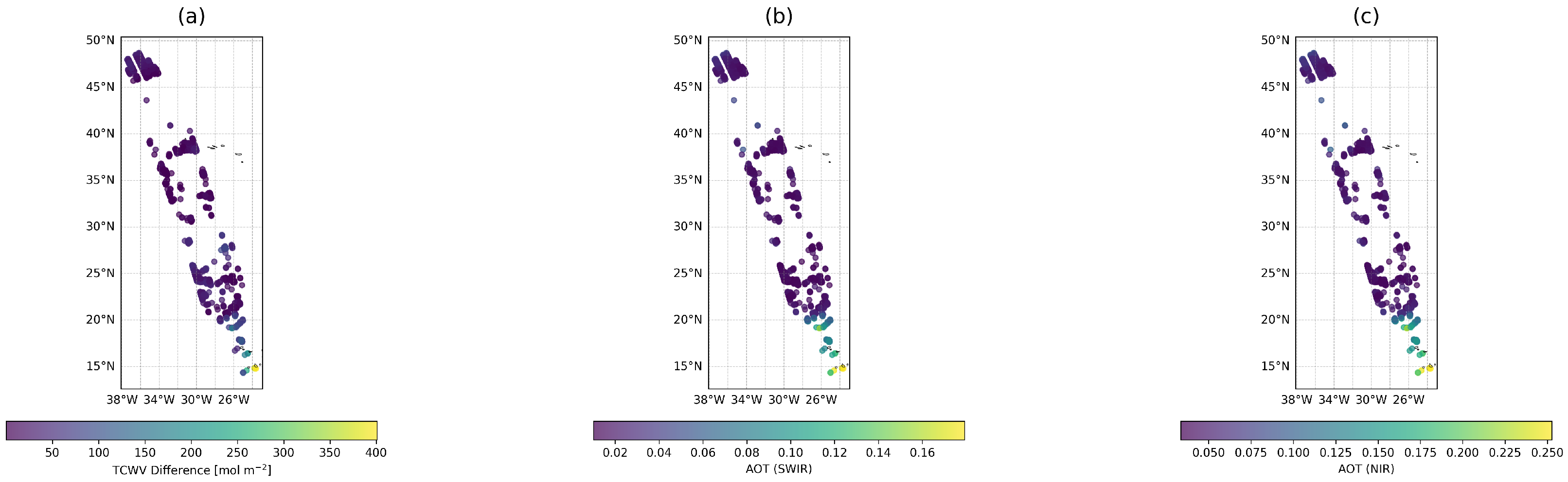
To investigate whether the parameters predicted by the classification model correlate with the outlier values observed in the eastern Atlantic Ocean, the spatial distributions of TCWV differences and AOT over this region are shown in Figure 6. The TCWV difference is defined as the residual between bias-corrected TCWV-FALCAS and TCWV-TROPOMI and represents the remaining retrieval error for each collocation. To create the TCWV difference map, the bias correction model was trained on the 70% training subset as described previously and then applied to the full dataset (training and test points) to visualise the entire regions. As the classification model identifies AOT in the SWIR and NIR ranges as dominant parameters, the high TCWV differences observed near 15°N, 26°W spatially coincide with elevated AOT values in both spectral ranges. This spatial correspondence suggests that enhanced aerosol loading is associated with increased retrieval errors in this region.

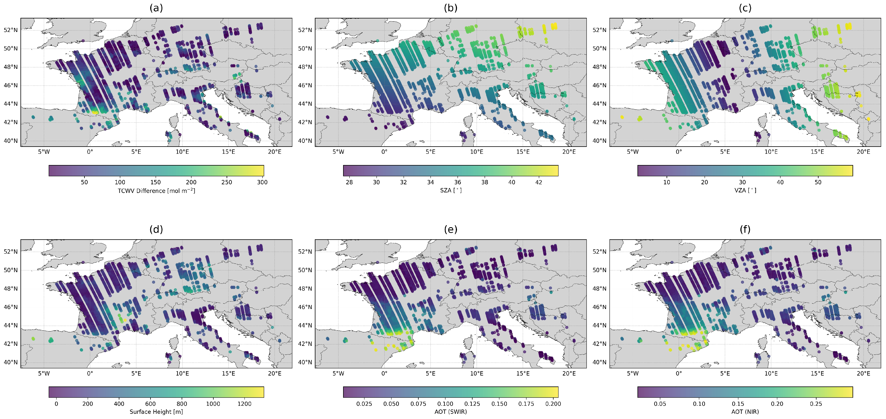
In contrast, the classification model does not clearly identify the parameter associated with the convex-like distortion observed over Europe. Figure 7 shows the spatial distributions of TCWV differences and selected auxiliary parameters over Europe. Although SZA, VZA, and surface height are ranked among the most important parameters by the classification model, the high TCWV differences observed near 43°N, 1°E do not spatially correspond to these parameters. Instead, panels (e) and (f) demonstrate that the high TCWV differences are closely associated with high AOT in both spectral ranges. This suggests that aerosol loading also contributes to the elevated retrieval errors observed in Europe.

The classification model successfully identifies the parameters associated with the outliers in the eastern Atlantic Ocean but fails to identify the convex-like distortion observed over Europe. In both cases, high AOT appears to be associated with the elevated TCWV differences. Although SZA and VZA are frequently ranked as important parameters influencing retrieval performance, spatial analysis indicates that locations with high SZA or VZA do not correspond to the areas with the largest localised errors. Additional regions were examined, and the same pattern was observed. It is worth noting that this observation is consistent with our previous research using synthetic data, where retrieval accuracy was found to gradually decrease as AOT increased.

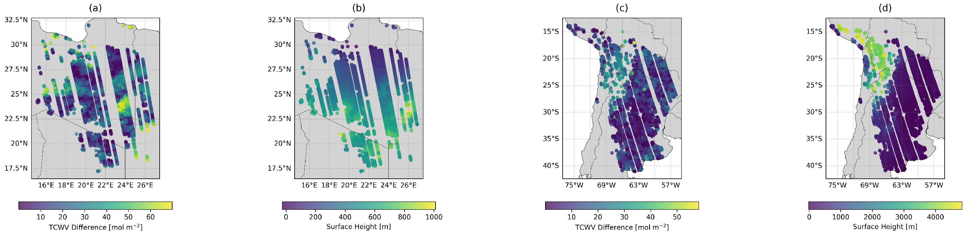
In North Africa and western South America, surface height is identified as an important parameter influencing retrieval accuracy. Although no large-scale systematic errors are apparent in these regions, the spatial distributions of TCWV differences and surface height are further examined in Figure 8.

In North Africa (panels a–b), areas with surface heights around 1000 m (near 22.5°N, 26°E) do not exhibit a clear correspondence with TCWV differences. In contrast, western South America shows a consistent relationship: regions with surface heights near 4000 m (around 20°S, 69°W) exhibit TCWV differences of approximately 40 mol m⁻². Although surface height does not appear to cause large-scale systematic errors, it can contribute to TCWV differences of up to 40 mol m⁻² in regions of extreme elevation, such as western South America.

In the current FALCAS retrieval framework, surface height is not included as a retrieval parameter because it is not directly provided in TROPOMI Level-1B data. For the error analysis, surface height is obtained from the ETOPO 2022 global topography dataset (30-arcsecond resolution). These findings suggest that incorporating surface height into the FALCAS forward model could further improve TCWV retrieval accuracy in high-elevation regions.

4. Discussion

Among the applied pre-processing criteria, the threshold on the number of defective spectral channels has the strongest impact on data availability. Our analysis shows that retrieval accuracy systematically decreases with increasing numbers of defective channels, although the sensitivity is region-dependent. Over Europe, retrieval accuracy remains comparable for up to five defective channels, whereas over North Africa a noticeable degradation is observed under the same condition. Consequently, the current filtering strategy retains approximately 33% of the available observations. Further analysis could therefore focus on region-specific threshold optimisation or adaptive quality filtering to increase retrieval availability while maintaining accuracy.

As observed in the regional correlation plots, the TCWV retrieval shows a high Pearson correlation coefficient (0.99) with TROPOMI data; however, the slope of the regression line exceeds unity and a small offset is present. Since our retrieval values are plotted on the y-axis, this indicates that FALCAS tends to overestimate TCWV at higher water vapour columns.

This overestimation is likely caused by systematic differences in the retrieval approaches. While FALCAS minimises the spectral residuals without additional regularisation, the TROPOMI reference products are retrieved using Philips–Tikhonov regularisation to constrain the solution towards the a priori state vector. Furthermore, the current FALCAS forward model simulates aerosol optical thickness only within the SWIR spectral range. This means that, when performing retrievals, FALCAS accounts for aerosols only at the target SWIR wavelengths. In contrast, TROPOMI retrievals use both NIR and SWIR bands simultaneously. The reason is that NIR wavelengths are more sensitive to aerosols due to stronger scattering, which allows the retrieval algorithm to constrain the aerosol amount more accurately. Similar discrepancies between satellite retrieval products have been reported in the literature and are often attributed to differences in forward modelling, inversion strategies, and calibration uncertainties [32].

Improving the FALCAS forward model by extending aerosol simulations to the NIR spectral range is expected to reduce the observed overestimation of TCWV at higher water vapour columns. Additionally, exploring alternative retrieval approaches, such as including regularisation terms similar to Philips–Tikhonov methods, could improve the accuracy of the retrieved water vapour values. Implementing these improvements is planned as part of future work.

We investigated whether TCWV could be retrieved from Sentinel-2 data. This band combination is widely used in operational TCWV products, which motivated our test. However, unlike hyperspectral instruments, Sentinel-2 provides only discrete multispectral measurements. Specifically, Sentinel-2 retrieves TCWV using the B09 (940 nm) water vapour absorption band together with the B08A (865 nm) reference band within a look-up table (LUT)-based retrieval framework. When applying the FALCAS retrieval approach—which is designed for hyperspectral measurements—to Sentinel-2 data, only two spectral points (B08A and B09) are available for the inversion. This severely limits the information content of the measurement vector. As a result, the inversion was found to be unstable and did not yield sufficiently accurate TCWV estimates.

To assess the validity of TCWV retrieved from the CH₄ product of Sentinel-5 Precursor, a comparison with TCWV derived from Sentinel-2 data was attempted. However, direct matching was challenging. The substantial difference in spatial resolution—kilometre-scale footprints for Sentinel-5P versus metre-scale pixels for Sentinel-2—introduces significant spatial-scale mismatch, particularly in scenes with heterogeneous surface or humidity conditions. Consequently, the substantial spatial-scale mismatch restricted the number of valid collocation points, and the comparison of these selected locations still exhibited low correlation.

5. Conclusions

In our study, TCWV is retrieved from TROPOMI Level-1B data using the FALCAS forward model, with the residuals between FALCAS and TROPOMI spectra minimised through a quasi-Newton BFGS inversion algorithm employing a multistart strategy. Thirteen regions were selected for the period June–August 2021, and the retrieval results were evaluated for consistency with the operational TROPOMI Level-2 TCWV product derived from the CH₄ retrieval. As this comparison is based on an operational product from the same instrument, it represents an intercomparison rather than a validation against an independent reference dataset, and the reported agreement reflects consistency rather than absolute accuracy.

The retrieval shows a high agreement with the operational TROPOMI TCWV product: the Pearson correlation coefficient between TCWV-TROPOMI and TCWV-FALCAS exceeds 0.99 for most regions. However, in the regional correlation plots, the retrieval is slightly overestimated, particularly at high TCWV, and a small offset is also observed. After empirical bias correction, the mean absolute bias across all regions is reduced to 1.45 mol m⁻² (0.12% relative) and the mean RMSE to 39.24 mol m⁻² (3.85% relative), representing a substantial improvement over the raw data values of 91.3 mol m⁻² (8.8% relative) and 118.2 mol m⁻² (10.7% relative), respectively. In the regional correlation plots after bias correction, a few outliers are observed in the eastern Atlantic Ocean, and a convex-like distortion appears over Europe. The retrieval errors in both regions are associated with high aerosol optical thickness.

Future work will focus on improving the FALCAS forward model by extending aerosol simulations to the NIR spectral range and exploring enhanced retrieval strategies, including regularisation techniques. Furthermore, it is of interest to incorporate empirical corrections accounting for cloud adjacency effects into the FALCAS processing pipeline [33]. These improvements are expected to further increase the accuracy of TCWV retrievals and reduce the overestimation observed at higher water vapour columns.

References

- Held, I.M.; Soden, B.J. Water Vapor Feedback and Global Warming. Annu. Rev. Energy Environ. 2000, 25, 441–475. [Google Scholar] [CrossRef] [Scilit]
- Vonder Haar, T.H.; Bytheway, J.L.; Forsythe, J.M. Weather and climate analyses using improved global water vapor observations. Geophys. Res. Lett. 2012, 39, L15802. [Google Scholar] [CrossRef] [Scilit]
- Veefkind, J.; Aben, I.; McMullan, K.; Forster, H.; de Vries, J.; Otter, G.; Claas, J.; Eskes, H.; de Haan, J.; Kleipool, Q.; et al. TROPOMI on the ESA Sentinel-5 Precursor: A GMES mission for global observations of the atmospheric composition for climate, air quality and ozone layer applications. Remote Sens. Environ. 2012, 120, 70–83. [Google Scholar] [CrossRef] [Scilit]
- Peraiah, A. An Introduction to Radiative Transfer: Methods and Applications in Astrophysics; Cambridge University Press: Cambridge, UK, 2001. [Google Scholar] [CrossRef] [Scilit]
- Hasekamp, O.; Lorente, A.; Hu, H.; Butz, A.; aan de Brugh, J.; Landgraf, J. Algorithm Theoretical Baseline Document for Sentinel-5 Precursor Methane Retrieval; Technical Report SRON-S5P-LEV2-RP-001; KNMI: De Bilt, The Netherlands, 2021. [Google Scholar]
- Lorente, A.; Borsdorff, T.; Martinez-Velarte, M.C.; Butz, A.; Hasekamp, O.P.; Wu, L.; Landgraf, J. Evaluation of the methane full-physics retrieval applied to TROPOMI ocean sun glint measurements. Atmos. Meas. Tech. 2022, 15, 6585–6603. [Google Scholar] [CrossRef] [Scilit]
- Afanas’ev, V.; Budak, V.; Efremenko, D.; Kaplya, P. Application of the Photometric Theory of the Radiance Field in the Problems of Electron Scattering. Light Eng. 2019, 27, 88–96. [Google Scholar] [CrossRef] [Scilit]
- Budak, V.P.; Smirnov, P.A. Quasi-diffuse approximation for calculation of light fields in 3D turbid media. Light Eng. 2025, 33, 73–79. [Google Scholar]
- Kokhanovsky, A.A. Asymptotic radiative transfer. In Light Scattering Reviews; Springer: Berlin/Heidelberg, Germany, 2006; pp. 253–289. [Google Scholar] [CrossRef] [Scilit]
- Kokhanovsky, A.; Natraj, V.; Efremenko, D. Analytical Methods in Radiative Transfer; Wiley: Hoboken, NJ, USA, 2025. [Google Scholar] [CrossRef] [Scilit]
- Ambartzumyan, V.A. The Effect of the Absorption Lines on the Radiative Equilibrium of the Outer Layers of the Stars. Publ. Obs. Astron. Univ. Leningr. 1936, 6, 7–18. [Google Scholar]
- Goody, R.; West, R.; Chen, L.; Crisp, D. The correlated-k method for radiation calculations in nonhomogeneous atmospheres. J. Quant. Spectrosc. Radiat. Transf. 1989, 42, 539–550. [Google Scholar] [CrossRef] [Scilit]
- Fomin, B.; Correa, M.P. A k-distribution technique for radiative transfer simulation in inhomogeneous atmosphere: 2. FKDM, fast k-distribution model for the shortwave. J. Geophys. Res. Atmos. 2005, 110, D02106. [Google Scholar] [CrossRef] [Scilit]
- Natraj, V.; Shia, R.L.; Yung, Y.L. On the use of principal component analysis to speed up radiative transfer calculations. J. Quant. Spectrosc. Radiat. Transf. 2010, 111, 810–816. [Google Scholar] [CrossRef] [Scilit]
- Natraj, V.; Spurr, R.J. Accelerating radiative transfer calculations in the thermal infrared through principal component analysis of inherent optical properties. J. Quant. Spectrosc. Radiat. Transf. 2025, 339, 109415. [Google Scholar] [CrossRef] [Scilit]
- del Águila, A.; Efremenko, D.S.; Molina García, V.; Kataev, M.Y. Cluster Low-Streams Regression Method for Hyperspectral Radiative Transfer Computations: Cases of O2 A- and CO2 Bands. Remote Sens. 2020, 12, 1250. [Google Scholar] [CrossRef] [Scilit]
- Águila, A.d.; Efremenko, D.S. Accuracy Enhancement of the Two-Stream Radiative Transfer Model for Computing Absorption Bands at the Presence of Aerosols. Light Eng. 2021, 29, 79–86. [Google Scholar] [CrossRef] [Scilit]
- Doicu, A.; Doicu, A.; Efremenko, D.S.; Loyola, D.; Trautmann, T. An Overview of Neural Network Methods for Predicting Uncertainty in Atmospheric Remote Sensing. Remote Sens. 2021, 13, 5061. [Google Scholar] [CrossRef] [Scilit]
- Rao, L.; Efremenko, D.; Doicu, A.; Shi, C.; Yin, S.; Letu, H.; Xu, J. Physics-Constrained Bayesian Neural Networks for Aerosol Retrieval From Hyperspectral Satellite Measurements With Integrated Uncertainty Quantification. IEEE Trans. Geosci. Remote Sens. 2025, 63, 4113918. [Google Scholar] [CrossRef] [Scilit]
- Verrelst, J.; Morata, M.; García-Soria, J.L.; Sun, Y.; Qi, J.; Rivera-Caicedo, J.P. RTM Surrogate Modeling in Optical Remote Sensing: A Review of Emulation for Vegetation and Atmosphere Applications. Remote Sens. 2025, 17, 3618. [Google Scholar] [CrossRef] [Scilit]
- Reuter, M.; Buchwitz, M.; Schneising, O.; Noël, S.; Rozanov, V.; Bovensmann, H.; Burrows, J. A Fast Atmospheric Trace Gas Retrieval for Hyperspectral Instruments Approximating Multiple Scattering—Part 1: Radiative Transfer and a Potential OCO-2 XCO2 Retrieval Setup. Remote Sens. 2017, 9, 1159. [Google Scholar] [CrossRef] [Scilit]
- Reuter, M.; Buchwitz, M.; Schneising, O.; Noël, S.; Bovensmann, H.; Burrows, J. A Fast Atmospheric Trace Gas Retrieval for Hyperspectral Instruments Approximating Multiple Scattering—Part 2: Application to XCO2 Retrievals from OCO-2. Remote Sens. 2017, 9, 1102. [Google Scholar] [CrossRef] [Scilit]
- Son, H.; Hochstaffl, P.; Efremenko, D. Surrogate infrared radiative transfer model for CO2 and CH4 retrieval. Light Eng. 2026, 34, 19–27. [Google Scholar]
- Schreier, F.; Gimeno García, S. Py4CAtS—Python tools for line-by-line modelling of infrared atmospheric radiative transfer. AIP Conf. Proc. 2013, 1531, 123–126. [Google Scholar]
- Schreier, F.; Gimeno García, S.; Hochstaffl, P.; Städt, S. Py4CAtS—PYthon for Computational ATmospheric Spectroscopy. Atmosphere 2019, 10, 262. [Google Scholar] [CrossRef] [Scilit]
- Efremenko, D.S.; Molina García, V.; Gimeno García, S.; Doicu, A. A review of the matrix-exponential formalism in radiative transfer. J. Quant. Spectrosc. Radiat. Transf. 2017, 196, 17–45. [Google Scholar] [CrossRef] [Scilit]
- Efremenko, D.; Pflug, B.; Richter, R.; de los Reyes, R.; Trautmann, T. Fast Computations of the Top-of-the-Atmosphere Radiance in a Spectral Range 400–2500 nm Using the PYDOME Tool. Environ. Sci. Proc. 2024, 29, 20. [Google Scholar] [CrossRef] [Scilit]
- Nocedal, J.; Wright, S. Numerical Optimization, 2nd ed.; Springer Series in Operations Research and Financial Engineering; Springer: New York, NY, USA, 2006. [Google Scholar]
- Smeets, J.; Kleipool, Q.; van Hees, R.; Sneep, M. Readme for TROPOMI Instrument Spectral Response Functions; Memo Document S5P-KNMI-OCAL-0149-ME; Royal Netherlands Meteorological Institute (KNMI): Utrecht, The Netherlands, 2018. [Google Scholar]
- Breiman, L. Random Forests. Mach. Learn. 2001, 45, 5–32. [Google Scholar] [CrossRef] [Scilit]
- NOAA National Centers for Environmental Information. ETOPO 2022 Global Relief Model; NCEI: Asheville, NC, USA, 2022. [CrossRef]
- Xu, J.; Wang, Y.; Chen, L.; Efremenko, D.; Rao, L.; Tana, G.; Liu, S.; Wang, Q.; Mao, J.; Wang, Y.; et al. First total ozone column observations from the Ozone Monitoring Suite-Nadir (OMS-N) onboard China’s FengYun-3F satellite. Sci. China Earth Sci. 2025, 68, 3665–3683. [Google Scholar] [CrossRef] [Scilit]
- Tarasenkov, M.V.; Engel, M.V.; Zonov, M.N.; Belov, V.V. Assessing the Cloud Adjacency Effect on Retrieval of the Ground Surface Reflectance from MODIS Satellite Data for the Baikal Region. Atmosphere 2022, 13, 2054. [Google Scholar] [CrossRef] [Scilit]
Figure 1.
Schematic of the OTIS layer representation in the FALCAS forward model. Multiple scattering is approximated using the FOCAL approach, summing contributions from all scattering paths between the OTIS level and the surface. Here,
b denotes the back-scattering fraction,
the surface albedo, and
the scattering optical thickness of the OTIS layer. Adapted from [
21].
Figure 2.
Correlation matrix of radiance derivatives with respect to the nine fitted state vector parameters. The derivatives were computed using a finite-difference approach by individually perturbing each parameter while keeping the others fixed, and evaluating the resulting change. The correlation matrix quantifies potential compensation effects between parameters, where values close to indicate strong correlation and values near 0 indicate weak correlation. The parameters shown in the matrix are: TCWV, XCH4, ground albedo (), albedo slope (), albedo curvature (), back-scattering fraction (), OTIS layer height (), Ångström turbidity (Åt) and Ångström exponent (Åe).
Figure 3.
TCWV correlation plots of TROPOMI (
x-axis) and FALCAS (
y-axis), shown separately for the regions defined in
Section 2.3.1. The red dashed line indicates the 1:1 relationship. The black text in each subplot shows the slope (a) and offset (b) of the linear fit (y = ax + b). The correlation coefficient (r) quantifies the strength and direction of the linear relationship between TROPOMI and FALCAS; values close to 1 indicate a strong positive correlation.
Figure 4.
Maps of TCWV retrieved from TROPOMI and FALCAS over China and eastern North America: (a) TROPOMI over China, (b) FALCAS over China, (c) absolute TCWV difference between FALCAS and TROPOMI over China, (d) TROPOMI over eastern North America, (e) FALCAS over eastern North America, and (f) absolute TCWV difference between FALCAS and TROPOMI over eastern North America. The colour scale is region-specific and indicates TCWV in mol m−2. In both regions, TCWV retrieved from FALCAS tends to be higher than that from TROPOMI in areas where TCWV exceeds 1500 mol m−2.
Figure 5.
Correlation plots of TCWV-TROPOMI (
x-axis) and TCWV-FALCAS (
y-axis) after bias correction, evaluated on the 30% independent test subset, shown separately for the regions defined in
Section 2.3.1. The black text in each subplot shows the slope (a), offset (b), and correlation coefficient (r) of the linear fit (y = ax + b) after bias correction. Outlier values remain in the eastern Atlantic Ocean, while in Europe deviations show a convex-like distortion around the middle of the diagonal.
Figure 6.
Spatial distribution of TCWV differences and aerosol optical thickness (AOT) over the eastern Atlantic Ocean. (a) Absolute difference between bias-corrected TCWV-FALCAS and TCWV-TROPOMI. (b) AOT in the SWIR spectral range. (c) AOT in the NIR spectral range. High TCWV differences near 15°N, 26°W spatially coincide with high AOT values.
Figure 7.
Spatial distributions of TCWV differences and selected auxiliary parameters over Europe. (a) Absolute difference between bias-corrected TCWV-FALCAS and TCWV-TROPOMI. (b) SZA. (c) VZA. (d) Surface height. (e) AOT in the SWIR spectral range. (f) AOT in the NIR spectral range. High TCWV differences near 43°N, 1°E are associated with enhanced AOT rather than geometric parameters and surface height.
Figure 8.
Spatial distributions of TCWV differences and surface height over North Africa and western South America. (a) Absolute difference between bias-corrected TCWV-FALCAS and TCWV-TROPOMI in North Africa. (b) Surface height in North Africa. (c) Absolute difference between bias-corrected TCWV-FALCAS and TCWV-TROPOMI in western South America. (d) Surface height in western South America. North Africa (∼1000 m) shows no clear relationship between elevation and TCWV differences, whereas western South America (∼4000 m) exhibits consistently high TCWV differences of approximately 40 mol m−2.