Performance and Detectability Analysis of Resident Space Objects Using an S-Band Bi-Static Radar with the Sardinia Radio Telescope as Receiver

Highlights

What are the main findings?

• A model-based feasibility analysis demonstrates the potential of using the Sardinia Radio Telescope (SRT) as a receiver in an S-band bi-static radar system for Resident Space Object (RSO) observations.
• The results show that the proposed configuration can detect RSOs with radar cross sections down to about 10⁻³ m² at several hundred kilometers and objects of 0.1–1 m² up to ~1700 km under realistic noise and interference conditions.

What are the implications of the main findings?

• Upgrading the BIRALET radar from P-band to S-band could significantly improve sensitivity, enabling the detection of smaller debris and extending the operational capabilities for space object monitoring.
• The study highlights the potential of large radio astronomy facilities such as SRT to operate as high-sensitivity receivers in bi-static radar systems supporting Space Situational Awareness (SSA).

Abstract

The continuous growth of the population of Resident Space Objects (RSOs) poses increasing challenges for Space Situational Awareness (SSA), particularly in terms of detection capability and collision risk mitigation. Ground-based radar systems represent a primary class of remote sensing instruments for RSO observation; however, their deployment is often constrained by cost and infrastructure requirements. In this context, the reuse of existing large radio astronomy facilities as radar receivers offers an innovative and potentially cost-effective alternative. This paper presents a fully model-based feasibility study of S-band bi-static radar observations of RSOs using the Sardinia Radio Telescope (SRT) as a high-sensitivity ground-based receiver. The analysis is entirely analytical and is conducted in the absence of experimental radar measurements. A bi-static radar equation framework is adopted to evaluate received signal power and the resulting signal-to-noise ratio (SNR) as functions of target size, range, and observation geometry. The model explicitly incorporates thermal noise, integration time and target dynamics, radio-frequency interference (RFI), atmospheric and environmental clutter contributions, and the realistic antenna radiation pattern of the SRT through a Gaussian beam approximation. Detection thresholds, maximum observable ranges, and performance envelopes are derived for representative RSO dimensions, and the impact of off-boresight reception on detectability is quantified. The results define the operational conditions under which RSOs may be detected in an S-band bi-static configuration and demonstrate the potential of the SRT as a non-conventional ground-based instrument for space object observation, supporting future developments in SSA and space debris monitoring strategies.

1. Introduction

The increasing number of Resident Space Objects (RSOs)—including active satellites, defunct spacecraft, and orbital debris—poses growing challenges for Space Situational Awareness (SSA) and collision risk mitigation [1,2,3]. As global reliance on satellite infrastructure expands, the ability to accurately detect, track, and characterize RSOs is critical for maintaining the safety and sustainability of space operations [4,5]. Ground-based radar systems play a fundamental role in SSA due to their ability to provide high-precision, all-weather, day-and-night observations of orbital parameters and object characteristics. This capability is particularly crucial in the increasingly congested Low Earth Orbit (LEO) region [6].

Globally, key ground-based radar facilities support the monitoring and tracking of RSOs, providing the foundation for regional SSA programs. In the United States, SSA capabilities are primarily managed by the Department of Defense through the Space Surveillance Network (SSN), a comprehensive system of ground-based radars, optical sensors, and space-based assets [7,8]. A key advancement in the SSN is the Space Fence system, operational since 2020 in the Marshall Islands. Using S-band radar (at approximately 3 GHz), Space Fence can detect objects as small as 0.01 m² in equivalent radar cross section (RCS) or 10 cm in diameter, significantly enhancing the monitoring of LEO traffic and debris [9,10].

Australia contributes to southern-hemisphere radar coverage in collaboration with allied programs, leveraging some of its radio telescopes. In particular, the Murchison Widefield Array (MWA) [11], a low-frequency (i.e., 70–300 MHz) radio telescope located at a radio-quiet site in Western Australia, serves as a radar receiver within a continent-spanning multi-static radar network for space surveillance, detecting all large objects (i.e., RCS greater than 1 m²) passing through its main beam within 1000 km [12].

Similar initiatives are undertaken in Europe, where SSA activities are coordinated by the European Space Agency (ESA) [13] and national agencies through the EU Space Surveillance and Tracking (EU SST) program [14]. Prominent facilities include the Tracking and Imaging Radar (TIRA), operated by Fraunhofer FHR in Germany, which features a 34 m dish with L-band tracking and Ku-band imaging capabilities, achieving high-precision range resolutions [15,16]. In a notable bi-static configuration, TIRA was combined with the 100 m Effelsberg radio telescope [17] as a receiving antenna, significantly improving detection sensitivity down to sub-centimeter-sized objects [18,19]. France contributes the GRAVES system, a bi-static radar operating at 143.050 MHz for continuous LEO monitoring [20,21]. ESA is also developing the German Experimental Space Surveillance and Tracking Radar (GESTRA), a phased-array system aimed at enhancing Europe’s autonomous tracking capabilities [22].

The MWA and Effelsberg campaigns highlighted that large radio telescopes, although primarily built for radio astronomy, can be successfully employed for space debris observations, providing precise measurements and confirming their value as versatile instruments for radar-based SSA [23].

Following the examples of other European countries, Italy has developed a significant SSA infrastructure, integrating civil and military resources to support both national and EU-wide objectives. The Bi-static Radar for LEO Survey (BIRALES) system exemplifies this approach. BIRALES employs a P-band transmitter (410–415 MHz) at the Salto di Quirra range in Sardinia and a multi-beam receiver array based on the Northern Cross Radio Telescope (with a bandwidth of 16 MHz at 410 MHz) at the Medicina radio astronomy station, near Bologna [24,25]. The receiver uses the BEST-2 array, providing a collecting area of ~2800 m² and a field of view of 6.6° × 2.2°. By synthesizing up to 32 simultaneous beams, BIRALES enables angular path reconstruction, Doppler shift analysis, and slant-range measurements, achieving accurate orbit determination from a single pass [26]. Detection sensitivity has reached equivalent RCSs as low as 0.13 m² at altitudes between 300 and 850 km, with recent pulse compression upgrades further enhancing range resolution [27].

Building on this survey capability, Bi-static Radar for LEO Tracking (BIRALET) extends the same bi-static concept by employing the 64 m Sardinia Radio Telescope (SRT) [28] as a high-gain receiver operating in the frequency window of 410–415 MHz, using its P-band cryogenic receiver [29]. The system is optimized for high-precision tracking and relies on a dedicated signal-processing backend for slant-range and Doppler measurements, enabling improved orbit reconstruction accuracy from targeted observations [30,31].

Both BIRALES and BIRALET played a significant role in supporting the Italian contribution to the monitoring of the uncontrolled re-entry of the Chinese space station Tiangong-1 in 2018. The systems were employed to enhance tracking accuracy and provide timely orbital updates, supporting national safety assessments in the event of a potential re-entry over Italian territory [32].

Beyond its role within the BIRALET frameworks in P-band, SRT has also been employed in X-band bi-static radar observations of Near-Earth Objects (NEOs), demonstrating its versatility and high sensitivity in planetary radar experiments [33]. Although primarily used as a scientific instrument for radio astronomy [34,35,36,37,38], this experience across both P- and X-band regimes confirms the SRT as a mature and reliable platform for bi-static radar applications.

Building on this background, the SRT represents a strong candidate for future S-band radar observations. In particular, a cryogenic multi-feed S-band receiver is currently under development, featuring seven feeds and operating over the 3–4.5 GHz frequency range [39]. The S-band provides reliable performance with good atmospheric penetration and is widely used in Europe for telemetry, tracking, and control, mobile satellite services, safety applications, multimedia delivery, and deep space missions [40]; however, these applications represent significant sources of radio-frequency interference (RFI) for radio-astronomical studies and may also affect radar observations conducted with radio telescopes [41]. A new S-band receiver for SRT will expand the operational capabilities of the telescope, further strengthening its role in radar-based observations of RSOs through improved sensitivity and survey flexibility.

This study investigates the feasibility of employing the SRT as a receiver in a bi-static S-band radar configuration for the detection of RSOs, adopting a fully model-based approach. The analysis evaluates received signal power and signal-to-noise ratio (SNR) as functions of target size, range, and observation geometry, explicitly accounting for thermal noise, radio-frequency interference, atmospheric and environmental clutter contributions, and the realistic antenna radiation pattern of the SRT modeled through a Gaussian beam approximation. Detection thresholds and maximum observable ranges are derived, and the impact of integration time and off-boresight reception on detectability is quantified. Although no experimental radar measurements are included, the resulting performance envelopes provide quantitative guidance for potential operational strategies, highlighting the role of the SRT as a non-conventional ground-based instrument for space debris monitoring and SSA.

2. Materials, Methods, and Simulation Framework

This section outlines the analytical methodology adopted in this study. In particular, Section 2.1 presents the system overview and bi-static radar geometry, including SRT as a passive receiver. Section 2.2 introduces the bi-static radar equation for estimating received signal power, while Section 2.3 describes the system noise model and instantaneous SNR. Section 2.4 considers the effects of integration time and target dynamics, and Section 2.5 characterizes the SRT antenna pattern and off-boresight losses. Section 2.6 addresses the issue of RFI in the band of interest, and Section 2.7 accounts for atmospheric and environmental clutter. Finally, Section 2.8 defines detection thresholds and the simulation framework for evaluating S-band bi-static radar performance against RSOs.

2.1. Bistatic Radar Geometry and System Concept

The observation concept considered in this study builds upon the heritage of the Italian BIRALET system, a P-band bi-static radar employed for space debris monitoring and tracking [30,31]. In the original implementation, a ground-based 7 m transmitter, named Radio Frequency Transmitter (TRF), illuminates the target while the 64 m SRT serves as a high-sensitivity receiver [30]. The baseline between transmitter and receiver is approximately 20 km, which is negligible with respect to typical target ranges of hundreds to thousands of kilometers. Consequently, the bi-static configuration can be approximated as quasi-monostatic for performance modeling purposes. The validation of this quasi-monostatic approximation is detailed in Section 3.1.

For this feasibility study, a conceptual upgrade of the system to S-band operation is assumed. The existing TRF infrastructure provides the mechanical and pointing capabilities necessary for high-precision tracking and could be adapted for S-band operation by designing and developing an appropriate feed and radio-frequency chain. The maximum available transmitting power of the TRF at P-band is 10 kW [30], which is assumed as a reference for the S-band configuration to enable a direct feasibility assessment. The technical feasibility study of the entire TRF upgrade, which is beyond the scope of the present work, should follow established guidelines in the literature for the design of microwave components, such as the development of ad hoc S-band power amplifiers [42,43]. Similarly, the SRT is considered as a receiving instrument in the 2–4 GHz range using a new cryogenically cooled receiver currently under development [39], leveraging its large collecting area, active surface system, and low system noise, which make it particularly well suited for this type of observation [44,45].

Within this observation concept, the transmitter continuously illuminates the target during a pass, while SRT tracks the expected target trajectory using its standard pointing capabilities. From an operational standpoint, the bi-static configuration is influenced by the different tracking capabilities of the transmitting and receiving antennas. The TRF system can achieve pointing speeds of up to 3°/s, enabling agile target tracking, whereas the SRT antenna operates with lower but well-characterized slew rates, limited to 0.85°/s in azimuth and 0.5°/s in elevation. These constraints play a key role in defining the achievable observation geometry and the temporal evolution of the bi-static link [30,31].

Synchronization between the TRF and SRT is ensured through the use of GPS-disciplined oscillators, providing a common time and frequency reference. This approach is already implemented in the original BIRALET system, where both the transmitter and receiver chains, equipped with a URSP National Instrument board, are synchronized using a 10 MHz reference signal and a one pulse per second (1 PPS) signal derived from GPS, ensuring precise timing alignment and frequency stability [30].

The received signal is assumed to originate from coherent scattering by the RSO, characterized by an equivalent bi-static RCS. The resulting bi-static geometry—including the transmitter–target and target–receiver distances, as well as the off-boresight angles at the SRT—forms the basis for the analytical performance modeling presented in the following sections.

Regarding the co-visibility issue between the TRF and SRT, the observation geometry is determined using orbital prediction models based on Two-Line Element (TLE) data and SGP4 propagation [31]. This allows the identification of time windows during which both the transmitter and the SRT have simultaneous visibility of the target.

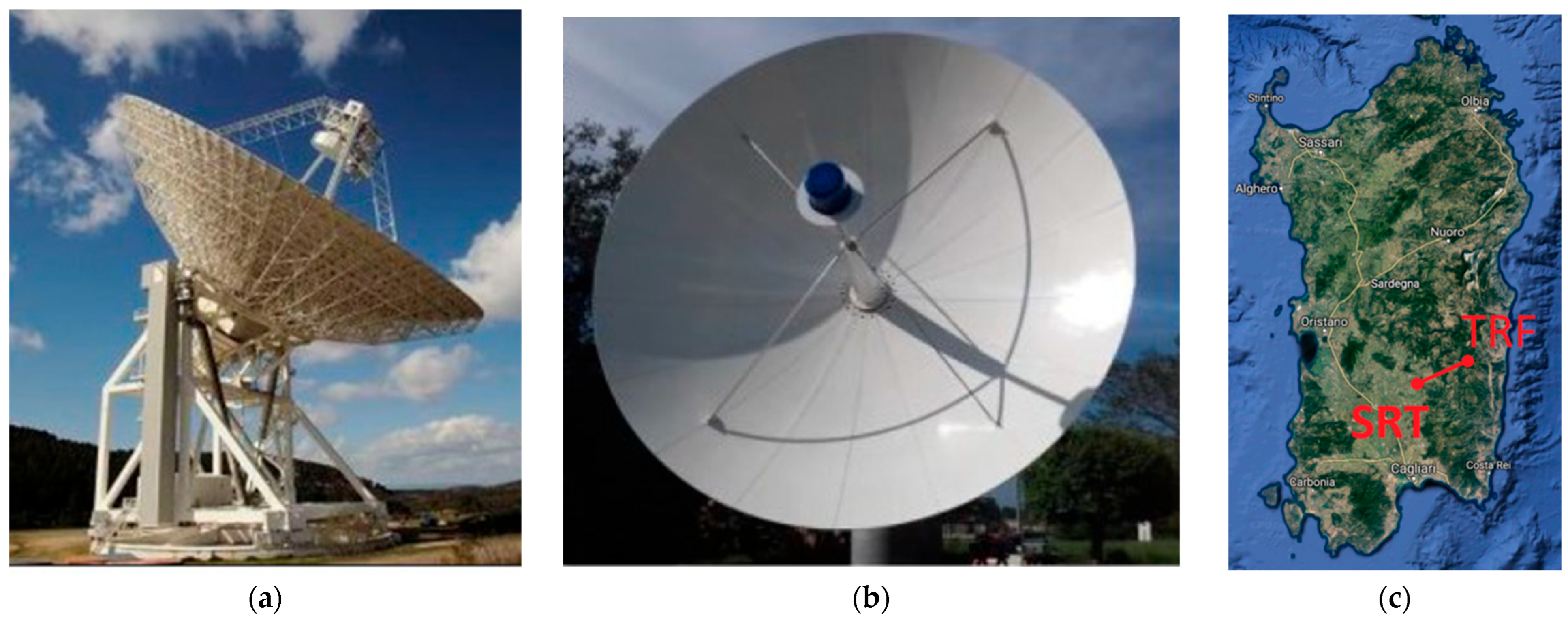
Figure 1 shows the SRT antenna, the TRF transmitting antenna, and a map of their locations in Sardinia, Italy, highlighting the ~20 km baseline used for bi-static observations.

Detailed technical descriptions of the TRF and SRT hardware, including the existing P-band receivers and transmission chain, are beyond the scope of this study. Interested readers can refer to [30,31] for comprehensive technical information.

2.2. Bistatic Radar Equation and Received Signal Power

The detection performance of this new proposed S-band radar configuration is assessed through a bi-static radar equation framework. In a general bi-static geometry, the transmitter and receiver are spatially separated, and the received echo power depends on the transmitter–target distance, the target–receiver distance, and the bi-static radar cross section (RCS) of the object.

The received power P_r can be expressed as [46]

$$P_r={\displaystyle \frac{P_t{G}_t{G}_r\left(\theta \right){\lambda }^2\sigma }{{\left(4\pi \right)}^3{R}_t^2{R}_r^2}},$$

(1)

where P_t is the transmitted power, G_t is the TRF antenna gain, G_r(θ) is the SRT receiving antenna gain as a function of the off-boresight angle θ, λ is the wavelength, and σ is the RCS of the target. The distances R_t and R_r represent the transmitter–target and target–receiver ranges, respectively.

For feasibility analysis, representative RCS values corresponding to typical RSO dimensions are considered [47]. The equation provides the basis for evaluating the received signal power as a function of target size, distance, and observation geometry. By combining the received power model with system noise contributions and detection thresholds, it becomes possible to derive detectability limits, maximum observable ranges, and minimum detectable object sizes for the proposed S-band bi-static configuration.

2.3. Noise Model and Signal-to-Noise Ratio

In this study, the system noise is modeled assuming thermal noise dominance, which represents a common and conservative assumption for S-band ground-based radar receivers operating with narrow bandwidths. The system noise temperature (T_sys) of a receiving antenna, such as SRT, combines the antenna temperature (T_A), which includes contributions from sky, ground, atmospheric emission, and possible RFI, with the receiver noise temperature (T_rec) [48].

Consequently, the system noise power is modeled as thermal noise according to [48,49]

$$N=k{T}_{sys}B,$$

(2)

where k is Boltzmann’s constant, Tsys is the system noise temperature, and B is the receiver bandwidth.

The signal-to-noise ratio (SNR) is computed as [49]

$$SNR={\displaystyle \frac{P_r}{N}},$$

(3)

where P_r is the received echo power obtained from the radar Equation (1) presented in Section 2.2.

This instantaneous SNR formulation represents the baseline performance metric used throughout the paper. Additional effects that enhance or degrade the effective SNR—such as coherent integration, target motion, antenna beam shape, and off-boresight reception—are addressed separately in the following sub-sections.

2.4. Integration Time and Target Dynamics

The detectability of RSOs is not determined solely by the instantaneous SNR, but also by the ability to coherently or incoherently integrate the received echo over a finite observation time [48]. For ground-based radar observations of objects in LEO, the achievable integration time is fundamentally limited by the relative motion between the target and the antenna beam.

In a beam-parking or fixed-pointing observation, the effective integration time is governed by the dwell time of the target within the main lobe of the receiving antenna. This dwell time T_int can be approximated as [48]

$$T_{int}\approx {\displaystyle \frac{{\theta }_{HPBW}}{\dot{\theta }}},$$

(4)

where θ_HPBW is the half-power beam width (HPBW) of the receiving antenna and θ˙ is the apparent angular velocity of the target as seen from the ground station.

For typical LEO objects, the apparent angular velocity is on the order of 0.5–1.5 degrees per second [50], while the S-band HPBW of the SRT at 3 GHz is on the order of fractions of a degree, as calculated in the following:

$${\theta }_{HPBW}\approx 1.22·{\displaystyle \frac{\lambda }{D}}=1.22·{\displaystyle \frac{0.1m}{64m}}=0.0019 rad=0.11°=6.55 arcmin.$$

(5)

As a result, integration times T_int of Equation (4) ranging from 10⁻² s to 10⁻¹ s may be achievable, depending on the observation geometry and pointing strategy.

Assuming coherent integration over N pulses, the resulting SNR improvement (SNR_int) can be expressed as [48]

$$SN{R}_{int}=SN{R}_{inst}·N,$$

(6)

where SNR_inst is the instantaneous SNR defined in Section 2.3. In practice, the maximum number of coherently integrable pulses is limited by Doppler frequency variations induced by target motion and by residual phase instabilities in the radar system.

When coherent integration is not fully achievable, incoherent integration may be adopted, yielding an SNR improvement proportional to √N. The choice between coherent and incoherent processing thus represents a trade-off between achievable sensitivity and robustness to phase errors [46].

In this study, integration effects are incorporated into the performance analysis by parameterizing the effective integration time and the corresponding number of pulses, allowing the evaluation of detectability as a function of target dynamics and observation strategy. It is worth noting that the above considerations primarily apply to beam-parking observations, where the antenna pointing is fixed and the integration time is limited by the target transit through the antenna’s main lobe.

On the other hand, in tracking mode, both the transmitting and receiving antennas dynamically follow the target trajectory, effectively removing the beamwidth-related constraint on the integration time. In this case, the achievable integration time is instead limited by factors such as ephemeris accuracy, residual pointing errors, Doppler frequency evolution, and phase stability of the radar system.

While tracking mode enables longer integration times and potentially higher SNR, the present analysis adopts a conservative approach by parameterizing the effective integration time independently of the pointing strategy. This allows the results to remain applicable to both beam-parking and tracking configurations.

2.5. Antenna Radiation Pattern of the Sardinia Radio Telescope

The antenna radiation pattern of the receiving system plays a critical role in determining the effective received power, particularly in bi-static radar configurations and during observations affected by pointing errors or beam-parking strategies. For large-aperture parabolic antennas such as SRT, the main lobe of the radiation pattern can be accurately approximated by a Gaussian function in the vicinity of the boresight [42].

Consequently, the receiving antenna gain of the SRT is modeled using a Gaussian beam approximation to account for realistic off-boresight reception effects. The angular-dependent gain G_SRT is expressed as

$$G_{SRT}\left(\theta \right)=G_0 exp\left[-4\ln \left(2\right){\left({\displaystyle \frac{\theta }{{\theta }_{HPBW}}}\right)}^2\right],$$

(7)

where G₀ is the on-axis gain and θ is the angular offset from the beam axis, and θ_HPBW is the half-power beamwidth, estimated in Equation (5).

This Gaussian approximation captures the dominant behaviour of the main lobe and is sufficient for performance estimation in feasibility studies, while side-lobe contributions are neglected. This assumption is justified by the focus on detection sensitivity rather than precise angular localization.

Off-boresight reception results in a reduction in the effective received power, which directly translates into an SNR degradation. The SNR as a function of angular offset, SNR(θ), can thus be expressed as

$$SNR\left(\theta \right)={SNR}_0 exp\left[-4\ln \left(2\right){\left({\displaystyle \frac{\theta }{{\theta }_{HPBW}}}\right)}^2\right],$$

(8)

where SNR₀ denotes the on-axis SNR.

In beam-parking observations, the angular offset θ varies with time as the target traverses the antenna beam, introducing a time-dependent SNR profile that limits the effective integration time. In tracking mode, residual pointing errors and ephemeris uncertainties may lead to a non-zero angular offset, which can be naturally incorporated into the same formulation.

The Gaussian beam model, therefore, provides a unified framework for quantifying beam-related losses in both beam-parking and tracking configurations, and it is adopted throughout the simulation framework described in Section 2.8.

2.6. Radio-Frequency Interference Effects

RFI represents a critical limiting factor for radar and, in general, radio astronomy observations conducted with highly sensitive radio astronomy receivers. This is particularly relevant in the S-band, where emissions from telecommunication systems, satellite downlinks, and other active services may overlap or partially contaminate the operational bandwidth [41]. Periodic RFI monitoring campaigns are routinely conducted at the SRT site to continuously assess and update the interference environment, accounting for contributions from both external sources in the surrounding territory and electronic systems installed on the antenna itself [51,52,53].

In the present study, RFI effects are not treated through a detailed spectral or spatial characterization, but are instead incorporated into the performance analysis using a simplified and conservative modeling approach. Specifically, RFI is accounted for through two complementary mechanisms: an effective increase in the system noise temperature and a reduction in the usable integration time due to data excision.

The impact of broadband or persistent interference is modeled as an increase in the effective system noise temperature T_sys,eff such that

$$T_{sys, eff}=T_{sys}+T_{RFI},$$

(9)

where T_RFI represents an equivalent noise temperature associated with interference contributions within the receiver bandwidth. This formulation allows RFI to be naturally included in the SNR definition introduced in the previous Section 2.3.

Transient or intermittent interference, on the other hand, is modeled as a reduction in the effective integration time. If a fraction η of the acquired data is discarded due to RFI mitigation or flagging, the effective number of integrated pulses is reduced accordingly, leading to a corresponding degradation of the achievable SNR.

This dual modeling approach captures the dominant effects of RFI on detection performance while remaining compatible with a fully analytical framework. Although no site-specific interference measurements are included in this study, the adopted parameterization enables sensitivity analyses under varying interference conditions and provides realistic performance bounds for S-band radar observations using the SRT.

2.7. Atmospheric and Environmental Clutter

Atmospheric and environmental clutter can affect radar observations through unwanted backscattering from the atmosphere, precipitation, or ground objects within the antenna side-lobes [46,54]. However, for S-band radar observations of RSOs in LEO, such contributions are generally expected to be significantly weaker than thermal noise and RFI effects [41,54].

In the considered observation geometry, the main antenna beam is directed well above the horizon, and the radar targets are located at ranges of several hundred to thousands of kilometers. Under these conditions, volume scattering from the troposphere and ionosphere contributes negligibly to the received power within the narrow receiver bandwidths typically adopted for space object detection.

Ground clutter may enter the receiver through antenna side-lobes, particularly during low-elevation observations. In this feasibility study, side-lobe related clutter is not explicitly modeled, as the analysis focuses on main-beam reception and adopts a Gaussian approximation for the antenna pattern, as described in Section 2.5. This assumption is consistent with the objective of deriving upper-bound performance estimates.

To account for residual environmental contributions in a conservative manner, atmospheric and environmental clutter effects are implicitly included in the system noise temperature T_sys [48]. This approach allows potential clutter contributions to be absorbed into an effective noise floor without introducing additional model complexity or requiring site-specific measurements.

The adopted treatment is appropriate for a model-based feasibility analysis and provides realistic performance bounds for S-band bi-static radar observations of RSOs using large radio astronomy facilities such as SRT. More detailed clutter characterization may be addressed in future studies supported by experimental measurements.

2.8. Simulation Framework and Performance Evaluation

The feasibility analysis presented in this work is supported by a numerical simulation framework developed in MATLAB R2018a [55], which integrates the analytical models introduced in the previous sections into a unified performance evaluation tool. The framework is designed to be fully parametric, enabling the systematic exploration of radar detectability as a function of system parameters, observation geometry, and target characteristics.

The received signal power is computed using the bi-static radar Equation (1) described in Section 2.2, incorporating the antenna gains of the transmitter and receiver, free-space propagation losses, and the assumed RCS of the target. The receiving antenna gain is further modulated by the angular offset-dependent pattern loss derived in Section 2.5.

The instantaneous SNR is evaluated according to the noise model introduced in Section 2.3, using a configurable system noise temperature T_sys and receiver bandwidth B. Integration effects are then applied following the formulation presented in Section 2.4, allowing both coherent and incoherent integration strategies to be modelled through an effective integration time or number of pulses.

RFI effects are included through the parameterization described in Section 2.6, either by increasing the effective system noise temperature or by reducing the usable integration time. Atmospheric and environmental clutter contributions are conservatively absorbed into the system noise budget, as discussed in Section 2.7.

For each simulated configuration, detection performance is assessed by comparing the resulting SNR with a predefined detection threshold. By varying target size, range, and observation geometry, the framework produces performance envelopes that define maximum detectable distances and minimum detectable RCSs under different operational assumptions.

The modular structure of the simulation framework allows individual effects to be enabled or disabled, facilitating sensitivity analyses and supporting future extensions based on experimental data. This approach ensures transparency and reproducibility, while maintaining consistency with the model-based nature of the present feasibility study.

3. Results

This section presents the results obtained using the simulation framework described in Section 2 and discusses their implications for S-band bi-static radar observations of RSOs using SRT as a receiver. As already mentioned, these results are based on a theoretical, model-driven framework, and real-world system performance may be affected by additional factors not fully captured in the analysis, such as hardware imperfections, calibration errors, and environmental variability. The analysis focuses on detection performance as a function of target size (i.e., RCS), range, and observation geometry. To support the validity of the adopted modeling approach, the analysis begins with an assessment of the quasi-monostatic approximation used throughout this work.

The discussion is structured across six sub-sections: Section 3.1 evaluates the validity of the quasi-monostatic approximation, Section 3.2 evaluates achievable SNR versus target size and range, Section 3.3 investigates the impact of integration time and target dynamics, Section 3.4 considers antenna pattern and off-boresight reception effects, Section 3.5 examines the influence of RFI and noise conditions, and Section 3.6 presents detection performance envelopes and a feasibility assessment. Together, these results highlight the combined influence of system parameters, observation strategies, and interference on RSO detectability with the SRT at 3 GHz.

3.1. Validation of the Quasi-Monostatic Approximation

The validity of the quasi-monostatic approximation adopted in this study was assessed by comparing the received power computed using the full bi-static radar equation with that obtained using the simplified formulation.

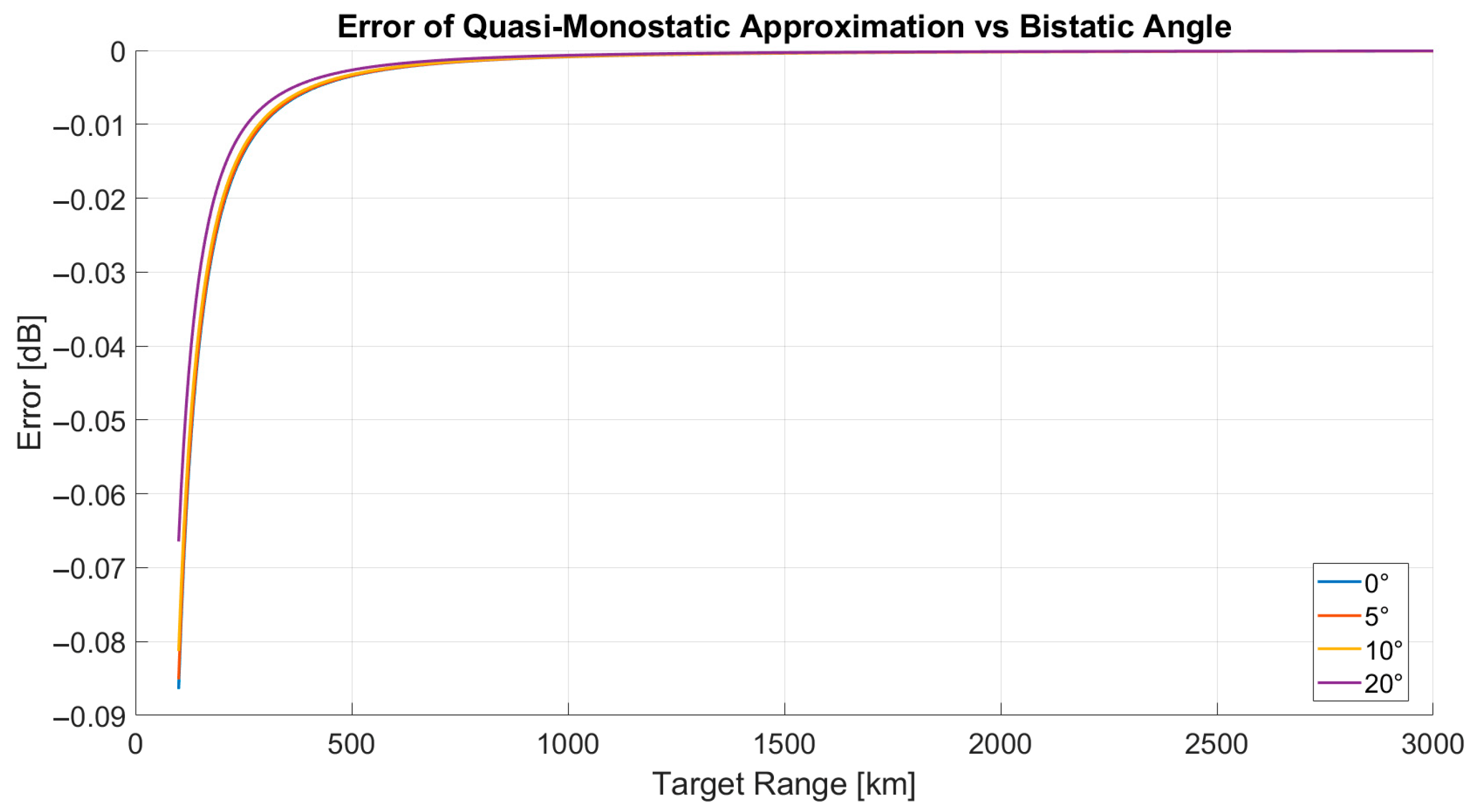
The analysis was carried out considering a transmitter–receiver separation of 20 km and target ranges between 100 km and 3000 km. In addition to the symmetric geometry (i.e., target located along the bisector of the baseline), the effect of non-zero bi-static angles was also evaluated by introducing angular offsets between the transmitter–target and receiver–target directions.

Figure 2 shows the difference between the two models in terms of received power for representative bi-static angles. The results indicate that, for small angular separations (up to approximately 10°), the quasi-monostatic approximation introduces a negligible error (well below 1 dB) over the entire range of interest. Even for larger bi-static angles (e.g., 20°), the deviation remains limited and decreases with increasing target distance.

Slight discrepancies are observed at shorter ranges and for larger angular offsets, where the bi-static geometry becomes more pronounced. However, these conditions correspond to non-nominal observation scenarios and fall outside the primary operational regime considered in this work.

Overall, the analysis confirms that the quasi-monostatic approximation provides a valid and computationally efficient representation of the bi-static geometry for typical observation conditions, supporting its use in the subsequent performance evaluation.

3.2. Signal-to-Noise Ratio as a Function of Target Size and Range

The first set of results evaluates the achievable SNR as a function of the target RCS and range. The received signal power is computed using Equation (1), and the corresponding SNR is derived according to Equations (2) and (3), assuming nominal system noise parameters. A monostatic-equivalent approximation is adopted, as the 7 m TRF and the 64 m SRT receiver are separated by only ~20 km. Therefore, the bistatic range is approximated by the distance between the target and the quasi-monostatic system. The analysis considers a system operating at 3 GHz, with a transmitter power of 10 kW, which represents the maximum offered by the existing TRF system at P-band [30]), a TRF antenna gain of 44.6 dBi (antenna efficiency of approximately 0.6 at 3 GHz [30,42]), an SRT antenna gain of 63 dBi (antenna efficiency of approximately 0.5 at 3 GHz [30,42]), a system temperature T_sys of 30 K (optimistic reference scenario, according to SRT C-band measurements reported in [36]), and a receiver bandwidth B of 1 MHz.

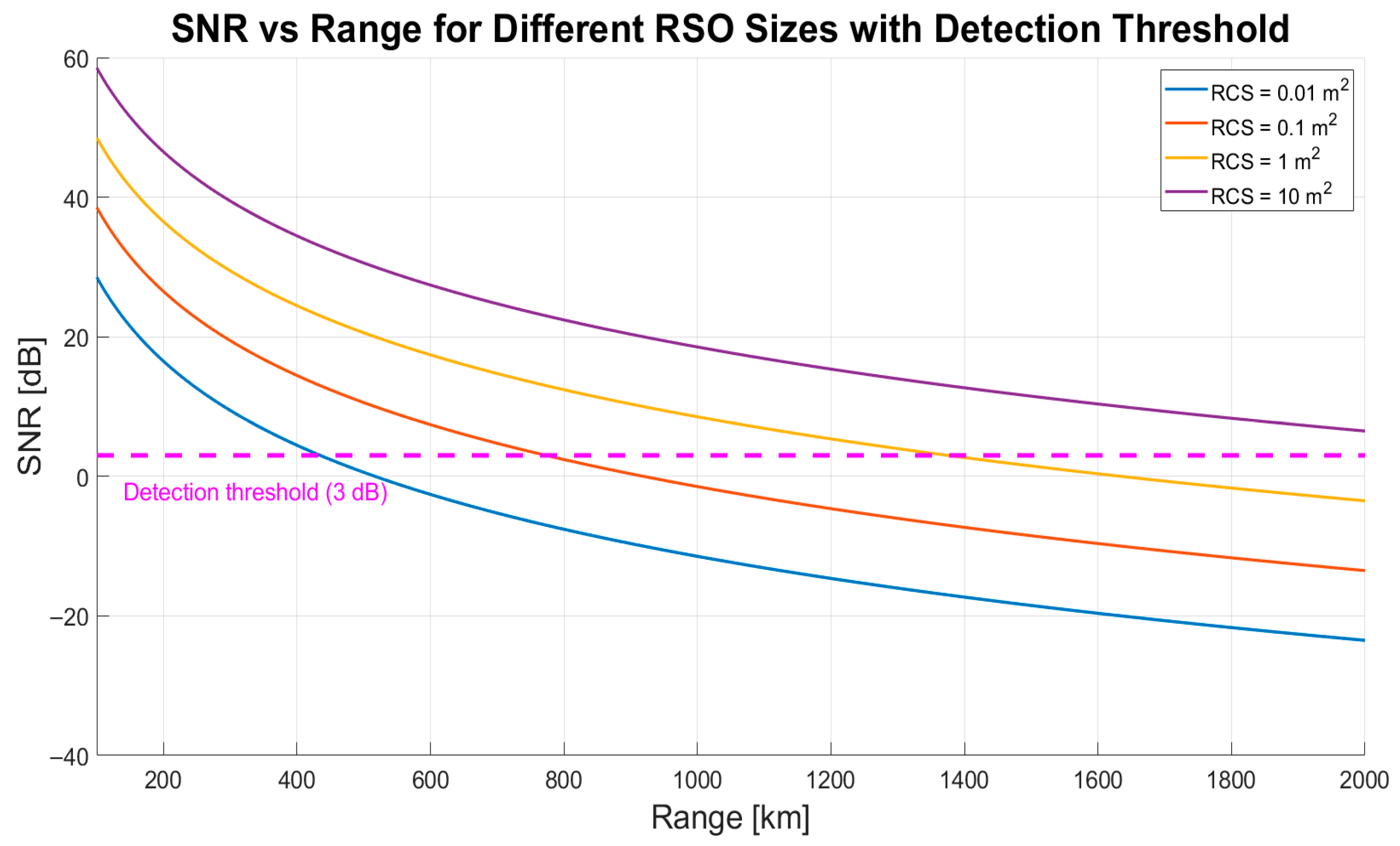
Figure 3 shows the resulting SNR as a function of target range for representative RSO sizes, based on the system parameters described above. The SNR decreases with increasing range due to free-space propagation losses. Notably, the S-band upgrade of the existing BIRALET radar allows the detection of small objects at significant distances: targets with an RCS of 0.01 m² are detectable with an SNR of approximately 3 dB at around 400 km. Medium-sized objects (RCS of 1 m²) can be observed up to 1400 km, while large targets (RCS of 10 m²) can be detected at ranges of 2000 km and beyond. These results highlight the trade-off between target size and maximum detectable range for S-band bi-static observations using large radio astronomy receivers.

The 3 dB threshold, highlighted in Figure 3, has been adopted as a reference sensitivity limit to evaluate the theoretical detectability of targets under ideal conditions. Consequently, this value may be optimistic in terms of detection reliability and false-alarm rate. Higher detection thresholds (e.g., 6 dB or above) would be more appropriate for robust operational scenarios, reducing the maximum detectable range, particularly for small RSOs.

3.3. Impact of Integration Time and Target Dynamics

The effect of signal integration is analyzed by varying the effective integration time calculated with Equation (4), accounting for both beam-parking and tracking observation strategies as described in Section 2.4.

The TRF of the BIRALET radar operates at 412.23 MHz with a frequency-modulated continuous wave (FMCW) chirp (410.43–414.03 MHz), using a pulse repetition frequency (PRF) of 50 Hz (i.e., pulse repetition interval of 20 ms) to enable accurate range measurements of debris up to 3000 km with approximately 30 m range accuracy [30]. These waveform characteristics justify the choice of the PRF and define the number of pulses available for integration. All the characteristics described above refer to the original P-band version of the TRF and can be extended to the case study of this paper, which considers the BIRALET system upgraded to S-band (i.e., 3 GHz). This choice ensures unambiguous range measurements and is consistent with the adopted radar waveform in P-band, while acknowledging that waveform optimization in S-band may require further investigation, which is beyond the scope of this paper.

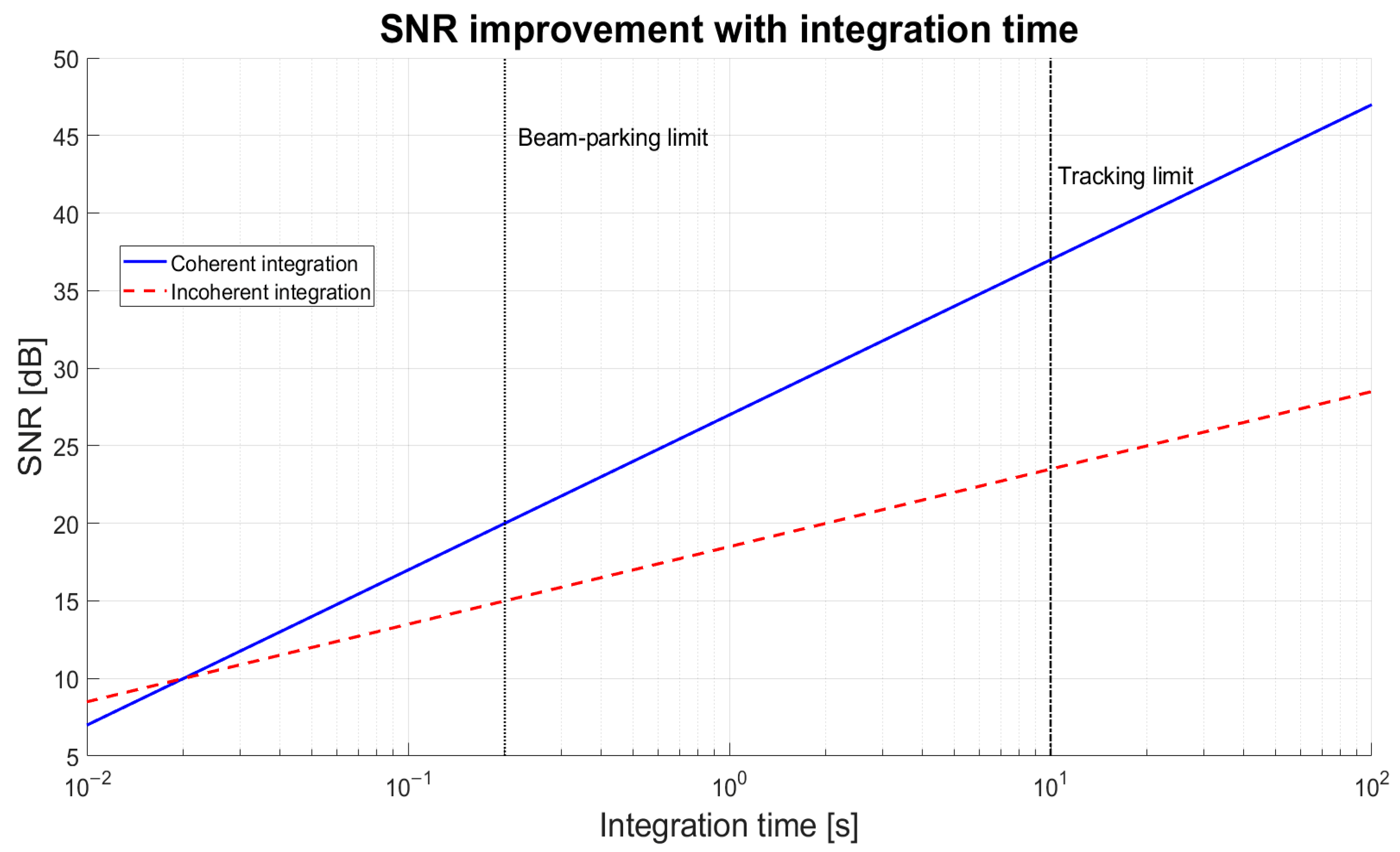
Figure 4 shows the resulting SNR improvement as a function of integration time for a fixed target size and range. Coherent integration provides an SNR gain proportional to the number of integrated pulses, while incoherent integration leads to a slower improvement proportional to the square root of the integration time [46].

The achievable integration time is ultimately constrained by target dynamics and system stability. In beam-parking mode, the integration time is limited by the dwell time of the target within the antenna HPBW. For the SRT antenna operating at 3 GHz, the HPBW is approximately 0.11°, as previously calculated in Equation (5), which, combined with the typical apparent angular velocity of LEO objects (of the order of 0.5–1.5 degrees per second [50]), results in a dwell time on the order of a few tenths of a second (0.2 s in Figure 4). Within this beam-parking limit, the SNR increases by approximately 10 dB for coherent integration and 5 dB for incoherent integration, as shown in Figure 4.

In tracking mode, longer integration times become feasible because the antenna continuously follows the target trajectory. However, the achievable coherent integration time is limited by Doppler variations, orbit prediction uncertainties, and overall system stability. As a result, coherent integration times of the order of seconds (10 s in Figure 4) and longer incoherent integrations are typically considered. Within this tracking limit, the SNR increases by approximately 30 dB for coherent integration and 20 dB for incoherent integration, as observed in Figure 4.

The results indicate that even modest integration times can significantly increase the achievable SNR and extend the detectable range for small RSOs, highlighting the importance of optimized integration strategies for bi-static radar observations using large radio astronomy receivers.

3.4. Effects of Antenna Pattern and Off-Boresight Reception

The influence of antenna pointing and beam pattern effects is investigated by evaluating the SNR as a function of angular offset from the antenna boresight, using the Gaussian beam model introduced in Section 2.5.

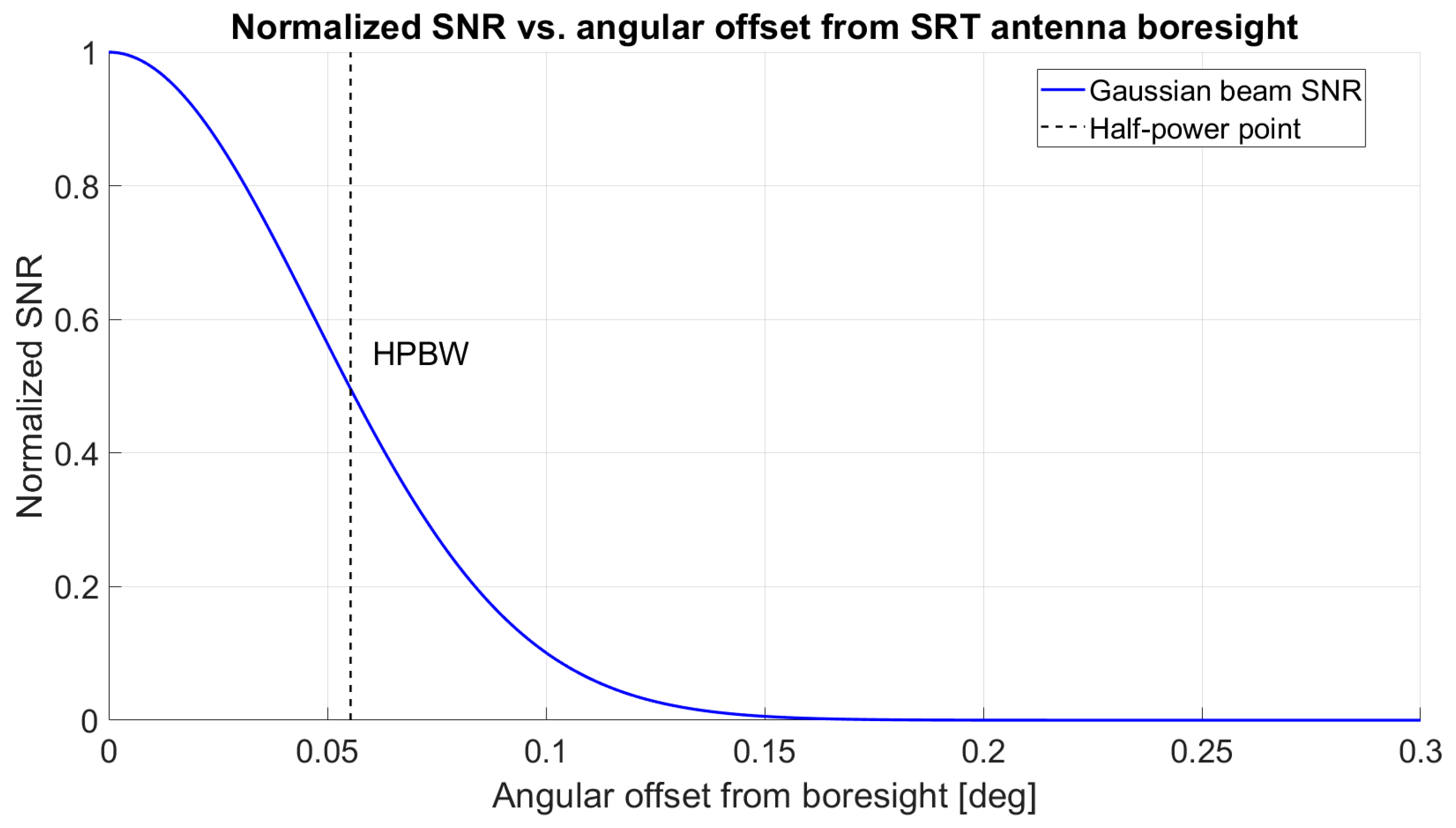
Figure 5 shows the normalized SNR degradation as a function of angular offset. A rapid decrease in SNR is observed as the target approaches the HPBW. For the SRT operating at 3 GHz, the HPBW is approximately 0.11°, implying that even small off-boresight angles can lead to significant losses in received signal power. This behavior highlights the strong sensitivity of system performance to pointing accuracy and tracking precision, particularly when observing small or distant RSOs.

In beam-parking observations, this effect produces a time-varying SNR profile as the target crosses the antenna beam, effectively reducing the useful integration time. In tracking mode, residual pointing errors translate directly into SNR penalties that must be considered in the overall system performance assessment.

Observations performed with the SRT in the 4.2–5.6 GHz frequency range have demonstrated a pointing accuracy better than one-tenth of the theoretical beam width [36]. This level of accuracy represents an excellent performance for RSO observations. A comparable pointing accuracy can reasonably be expected for the S-band case considered in this work (3 GHz), suggesting that the SNR degradation due to pointing errors is expected to remain limited under nominal operating conditions.

3.5. Influence of RFI and Noise Conditions

The sensitivity of detection performance to RFI is examined by varying the effective system noise temperature T_sys and the usable integration time, following the modeling approach described in Section 2.6. For this analysis, a target RCS of 1 m² is assumed, and coherent integration with 200 pulses is considered. The SNR threshold is set to 3 dB, consistent with the estimates reported in Section 3.2 (see Figure 3).

RFI affects radar sensitivity in two main ways: it increases the effective T_sys and may require the excision of contaminated data segments, effectively reducing the achievable integration gain. System noise temperatures ranging from 30 K (ideal case, used in Section 3.2 according to SRT C-band measurements reported in [36]) up to 400 K are considered to account for progressively stronger interference conditions.

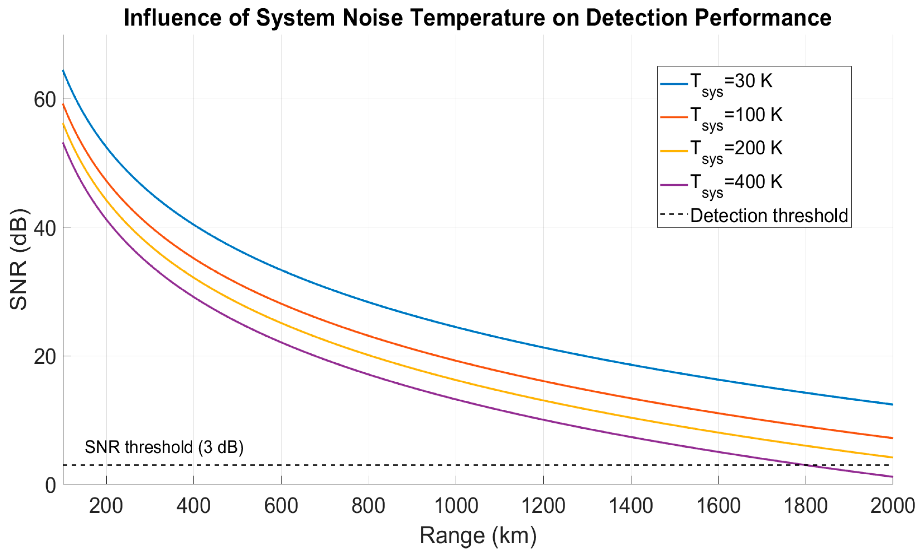
Figure 6 shows the resulting SNR as a function of range for different T_sys values. Even moderate increases in T_sys lead to a noticeable reduction in maximum detectable range. In the worst-case scenario (T_sys = 400 K), the target is detectable up to approximately 1800 km, while for T_sys = 200 K, the detectable range is about 2000 km. For lower noise temperatures (30 K and 100 K), the system enables observations at ranges exceeding 2000 km.

These results highlight the importance of RFI mitigation strategies and careful frequency planning when operating radio astronomy facilities as radar receivers in the S-band, and they provide a quantitative assessment of the impact of RFI and noise conditions on the detectability of RSOs. Periodic RFI measurement campaigns at SRT are necessary to keep RFI maps updated and ensure reliable observation planning, as done for other frequency ranges reported in [51,52,53].

3.6. Detection Performance Envelopes and Feasibility Assessment

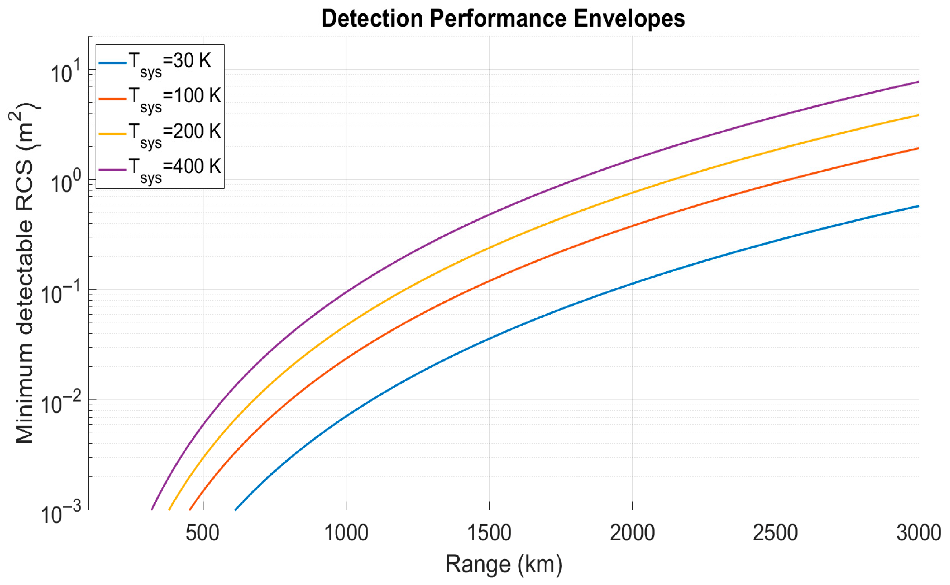
By combining all modeled effects, detection performance envelopes are derived that define the operational conditions under which RSOs of different sizes can be detected. For this analysis, coherent integration with 200 pulses is considered, the SNR threshold is set to 3 dB, and system noise temperatures ranging from 30 K (ideal case) up to 400 K (representative of severe RFI conditions) are evaluated.

Figure 7 summarizes the minimum detectable radar cross section as a function of range for these representative system configurations. Very small targets, with RCS as low as 10⁻³ m², can be observed at ranges of approximately 400 km even under moderate noise conditions (T_sys ≥ 100 K). Medium-sized objects, with RCS between 0.1 m² and 1 m², are detectable up to about 1700 km for high noise temperatures (T_sys = 400 K), indicating that the system retains good performance even in the presence of strong RFI. Large targets (RCS ≈ 10 m²) are detectable at ranges above 2000 km for low-noise conditions, and still up to 3000 km under T_sys = 400 K.

Overall, the envelopes clearly indicate the regimes in which S-band bi-static radar observations using the SRT are feasible, as well as the sensitivity margins associated with integration time and interference assumptions. Despite the absence of experimental radar data, the SRT shows strong potential as a non-conventional S-band radar receiver for space object observation. The presented analysis provides quantitative guidance for future experimental campaigns and system upgrades, supporting the role of large radio astronomy facilities in SSA and remote sensing applications.

4. Discussion

The results presented in Section 3 provide a quantitative assessment of the detection capabilities achievable with an S-band bi-static radar configuration using SRT as a receiver. By systematically analyzing the effects of target size, range, integration time, antenna pointing, and interference conditions, the study defines the operational regimes in which RSOs can be detected and observed using this configuration. The results also allow a direct comparison with the performance already demonstrated by the existing P-band BIRALET system, highlighting the potential benefits of upgrading the radar to operate in the S-band.

The original BIRALET radar operating in P-band has already demonstrated its capability to detect RSOs at significant distances. In particular, observation campaigns conducted between 2019 and 2020 showed that the system was able to detect RSOs with RCS values ranging from approximately 0.1199 m² to 12.1 m² at bi-static slant ranges between about 1200 km and 2600 km [30]. These experimental observations confirmed the feasibility of using a bi-static radar configuration based on the TRF and the SRT receiver for space object detection and tracking.

The model-based analysis carried out in this work indicates that upgrading the system to the S-band would significantly improve its sensitivity to smaller objects. The shorter wavelength associated with S-band operation increases the radar sensitivity and therefore enhances the capability to detect RSOs with smaller RCS values. As shown by the detection performance envelopes derived in Section 3, objects with RCS values as small as 10⁻³ m² may become detectable at ranges of several hundred kilometers. Medium-sized RSOs, with RCS between 0.1 m² and 1 m², can be observed at distances approaching 1700 km even under high system noise conditions, while larger objects remain detectable at ranges exceeding 2000 km. These results indicate a significant extension of the detectable RCS domain toward smaller debris compared to the operational performance previously achieved by the P-band BIRALET system.

These results indicate a significant extension of the detectable RCS domain toward smaller debris compared to the operational performance previously achieved by the P-band BIRALET system.

To better contextualize these findings, a comparison with representative international SSA radar systems is reported in

Table 1. Comparison between representative SSA radar systems and the proposed S-band bistatic configuration using SRT.

System	Frequency	Configuration	Antenna Size	Approximately Min Detectable RCS	Max Range
Space Fence	S-band (~3 GHz)	Monostatic (phased array)	Large phased array	~0.01 m2	>2000 km
TIRA/Effelsberg	L-/S-band	Bistatic/Monostatic	34 m/100 m	~0.01–0.1 m2	~1000–2000 km
GESTRA	L-band (~1.3 GHz)	Monostatic (phased array)	Array system	~0.1 m2	~1000 km
MWA-based radar	VHF (~100–300 MHz)	Passive/Bistatic	Array system	>1 m2	~1000 km
BIRALET (P-band)	~400 MHz	Bistatic (TRF + SRT)	7 m (Tx)/64 m (Rx)	~0.12–12 m2	~2600 km
Proposed S-band SRT system	~3 GHz	Bistatic (TRF + SRT)	7 m (Tx)/64 m (Rx)	~10−3–1 m2 *	~400–2000+ km

* Depending on system noise temperature, integration time, and RFI conditions.

. The comparison includes key parameters such as operating frequency, system configuration, antenna size, minimum detectable RCS, and maximum detection range.

The analysis shows that state-of-the-art systems such as Space Fence [9,10] and TIRA [15,16] achieve high detection performance thanks to dedicated high-power transmitters and large-scale antenna infrastructures. In contrast, the proposed S-band bi-static configuration based on SRT leverages an existing radio astronomy facility as a high-sensitivity receiver, offering a cost-effective alternative for space object observation. In addition, the inclusion of the existing P-band BIRALET system in Table 1 provides a direct reference for experimentally validated performance. The comparison clearly highlights the expected improvement achieved by the S-band upgrade, particularly in terms of sensitivity to smaller RSOs, while maintaining comparable detection ranges for larger objects.

Another important outcome of the analysis concerns the influence of observation parameters on detection performance. The results highlight the critical role of coherent integration in improving the achievable SNR and extending the detectable range for small RSOs. At the same time, accurate antenna pointing is required to avoid significant sensitivity losses caused by off-boresight reception, particularly when observing small or distant targets. The analysis also shows that RFI may substantially affect radar sensitivity by increasing the effective system noise temperature and reducing the achievable integration gain. These effects emphasize the importance of careful observation planning, accurate antenna tracking, and the adoption of RFI mitigation strategies when operating radio astronomy facilities as radar receivers.

Despite the promising results, it should be emphasized that the present study is entirely based on analytical modeling and does not rely on experimental radar observations in the S-band. Although realistic system parameters were adopted, several simplifying assumptions were introduced, including the quasi-monostatic approximation and the use of a Gaussian beam model for the antenna radiation pattern. Experimental validation will therefore be necessary to confirm the predicted detection performance under real observing conditions.

Overall, the results obtained in this study demonstrate the strong potential of using large radio astronomy facilities such as SRT as high-sensitivity receivers in bi-static radar systems for space object observation. In particular, the findings provide a strong motivation for pursuing the upgrade of the BIRALET radar to operate in the S-band, which would significantly enhance its capability to detect smaller RSOs and support future SSA activities.

5. Conclusions and Future Work

This study analyzed the technical specifications of the SRT in the S-band (3 GHz) to estimate its performance as a receiver in a bi-static radar configuration for RSO observations. By combining all modeled effects—including target RCS, range, integration time, antenna pattern, and RFI conditions—detection performance envelopes were derived, providing a comprehensive assessment of the operational regimes in which S-band bi-static observations with SRT are feasible.

The analysis shows that small RSOs (RCS ≈ 10⁻³ m²) can be detected at ranges of several hundred kilometers, medium-sized RSOs (RCS 0.1–1 m²) up to around 1700 km under high T_sys conditions, and large RSOs (RCS ≈ 10 m²) at distances exceeding 2000–3000 km. These results highlight the strong potential of SRT as a non-conventional S-band radar receiver for SSA, despite the absence of experimental radar data.

The study also demonstrates the critical role of integration time, accurate antenna pointing, and effective RFI mitigation in extending the detectable range and improving SNR for RSOs of various sizes. Detection envelopes and sensitivity margins derived in this work provide quantitative guidance for future observation campaigns, system upgrades, and feasibility studies of bi-static radar operations with large radio astronomy facilities.

Future Work will focus on incorporating more realistic scattering models, including aspect-dependent RCS and electromagnetic simulations, representing an important direction for improving the physical accuracy of the analysis. In addition, the effective discrimination of multiple RSOs within the same antenna beam will be investigated by considering advanced signal processing techniques such as range–Doppler separation and multi-target detection algorithms, which are required for realistic operational scenarios. Finally, the findings of this study will be exploited to support the upgrade of the existing Italian BIRALET radar from P-band to S-band. Such an upgrade would enable higher-resolution observations and improved detectability of small RSOs at extended ranges. Periodic RFI monitoring campaigns, system calibration, and experimental validation of the predicted detection envelopes will be essential to ensure reliable operation and refine performance estimates under real observational conditions.