Satellite-Based Differential Radar Interferometry in Landslide Research: An Overview of Applications and Challenges

Highlights

What are the main findings?

• Comprehensive spatiotemporal characterization: DInSAR has evolved from an experimental research tool to a sophisticated technology for the continuous monitoring of landslide dynamics, characterization, mapping, triggering and conditioning factors identification, model development, and asset impact assessment.
• Methodological synergy and AI integration: The current use of DInSAR for landslide research is shifting towards its integration with multi-source datasets (e.g., LiDAR, GNSS, and in situ data) and the application of artificial intelligence (AI) and advanced computer resources for the management and processing of massive regional datasets.

What are the implications of the main findings?

• Enhanced risk management: the improved accuracy and temporal resolution of DInSAR outcomes facilitate more precise susceptibility and hazard mapping, providing essential data for land-use planning and the design of effective mitigation strategies.
• Advancement toward quasi-early warning systems: the transition toward quasi-real-time processing and the upcoming next-generation satellite missions are bridging the gap between historical analysis and the implementation of operational quasi-real-time early warning systems for landslide prevention.

Abstract

The use of satellite Differential Synthetic Aperture Radar Interferometry (DInSAR) has transformed the analysis of landslide dynamics by enabling detailed spatiotemporal monitoring of slow and subtle ground deformations. DInSAR enables comprehensive geomorphological characterization and identification of triggering factors. Retrospective applications of DInSAR provide valuable insights into past events and support causal analysis linked to rainfall episodes or piezometric fluctuations. Moreover, integration with numerical modeling enhances predictive capabilities and facilitates the calibration of geotechnical parameters. DInSAR is also instrumental in assessing infrastructure impacts and in the generation of susceptibility, hazard, vulnerability, and risk maps, which are key for land-use planning and risk management. Nevertheless, this technique has inherent limitations that must be carefully considered when interpreting results. Future developments, driven by the integration of artificial intelligence and enhanced computing capacities, are transforming the landscape of InSAR applications in landslide studies. These advancements, combined with upcoming satellite missions, are expected to significantly improve measurement accuracy, temporal resolution, and overall operational potential, paving the way for more robust quasi-early warning systems for landslide prevention. In this work, an overview of the current applications, future trends, and challenges of DInSAR in landslide studies is presented, with particular emphasis on the practical dimension of landslide studies and on the exploitation of DInSAR outcomes to support risk management and mitigation strategies.

1. Introduction

Detailed landslide investigations typically involve surface data acquisition (e.g., geomorphological analysis), subsurface exploration (e.g., boreholes and geophysical surveys), and the monitoring of key variables involved in slope instability processes (e.g., surface and subsurface displacements and piezometric levels) [1,2]. Traditionally, a wide range of topographic, geodetic, and instrumental methods has been employed for monitoring purposes. However, since the 1990s, there has been a significant increase in the number of Earth observation satellites in orbit, a trend that has accelerated in the 21st century [3]. This expansion has been paralleled by the development of numerous applications and methodologies aimed at leveraging the data provided by these satellites.

Although the first synthetic aperture radar (SAR) satellite—Seasat—was launched in 1978, it was not until the launch of the ERS-1 and ERS-2 satellites by the European Space Agency in 1991 and 1995, respectively, that the practical implementation of Differential SAR Interferometry (DInSAR) became feasible [4,5]. In essence, this technique allows for the comparison of two or more SAR images of the same area to detect subtle changes in the distance between the satellite and the ground surface, thereby enabling precise measurement of ground deformation over time [6,7,8]. Later developments led to substantial improvements in processing, culminating in a family of advanced techniques collectively referred to as Multitemporal DInSAR (MT-DInSAR). These methods rely on a large archive of SAR images to identify specific radar targets—Persistent Scatterers (PS) and/or Distributed Scatterers (DS)—whose phase information remains stable or coherent over time, allowing high-precision displacement estimates, while excluding areas with low signal stability [9]. This technique produces time series of ground motion for the selected area, making it possible to analyze both the spatial-temporal evolution of displacement fields and the temporal behavior of individual measurement points (MPs) [10,11].

InSAR’s wide spatial and temporal coverage, combined with its remote sensing capabilities—i.e., the absence of a need for physical access to the monitored area—make it a highly valuable tool for landslide research in difficult-to-access contexts, ranging from urban areas [12] to mountainous regions [13].

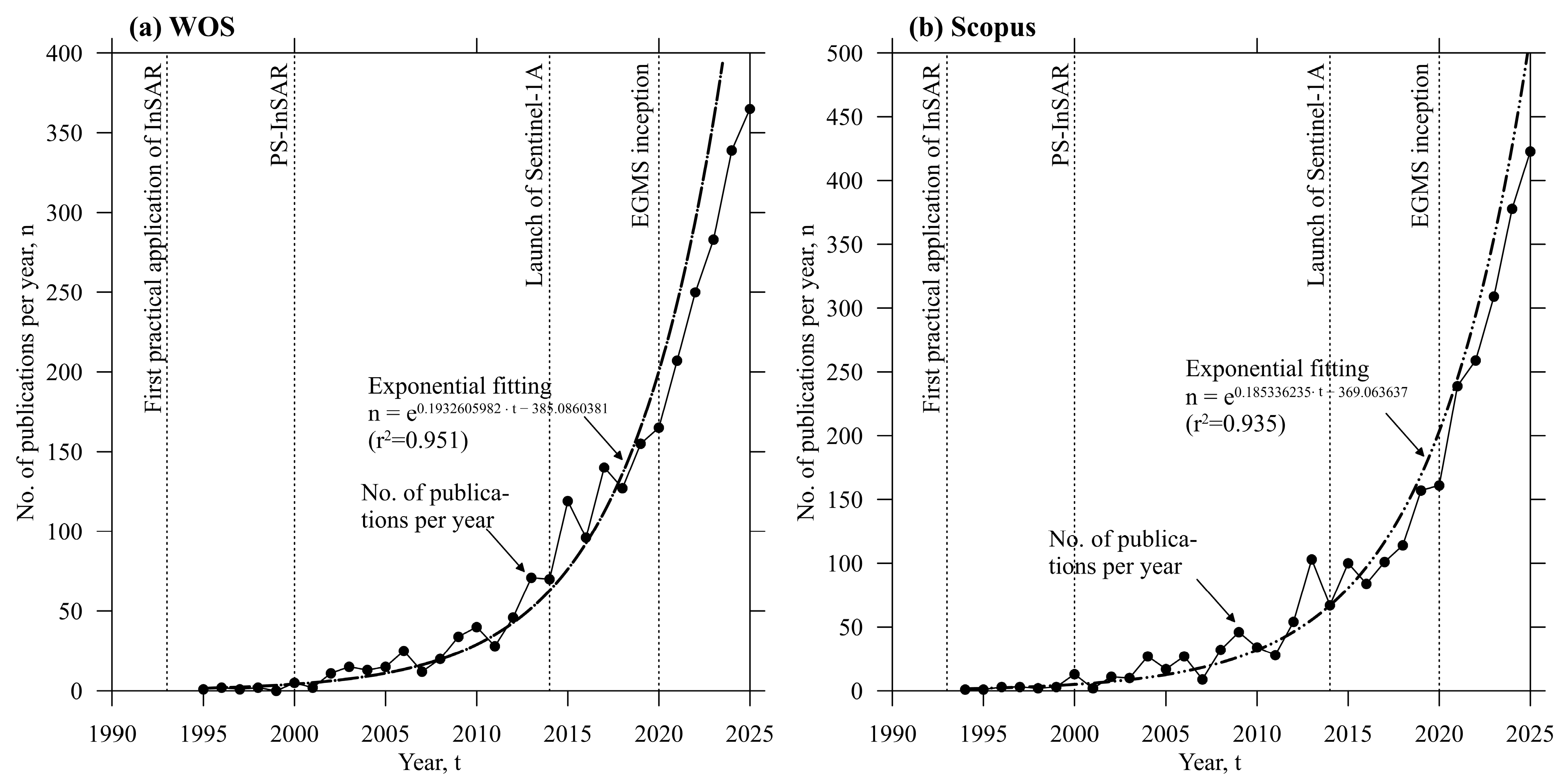
To assess the evolution of DInSAR usage in landslide studies, we conducted a basic bibliometric analysis, applying a different set of search criteria. Figure 1 presents the temporal distribution of publications indexed in all Web of Science (WOS) and Scopus databases using the following search terms in the “topic” field for the WOS and “Article title, Abstract and Keywords” for Scopus: “SAR interferometry” OR “InSAR” OR “Synthetic aperture radar interferometry” OR “PSInSAR” AND “landslide*” OR “mass movement*” OR “slope failure*”, up to year 2025. The wildcard character (*) was used to capture variations of the search terms. The figure also highlights key milestones in the evolution of DInSAR, such as the development of PS-InSAR techniques and the launch of the Sentinel-1A satellite, which have clearly driven progress in the field.

The search, conducted in February 2026, returned a total of 2886 and 2713 records in the Web of Science and Scopus databases, respectively. The first documented application of DInSAR to landslide monitoring [14] was published in a conference two years after the first operational use of satellite DInSAR to analyze the 1992 Landers earthquake [15], which featured on the cover of Nature. However, the first journal paper related to these topics was published in 1993. Since then, the global trend in publications matching the defined search criteria has shown pure exponential growth (Figure 1), reaching a peak of 365 and 423 articles published in 2025 in WOS and Scopus, respectively.

The analysis of the Scopus dataset conducted via VOSviewer version 1.6.20 [16] identifies current research hotspots in InSAR-based landslide monitoring as being concentrated in China and Italy, led by authors from these countries (Figures S1 and S2). The evolution of trends, as revealed by the overlay visualization, shows a significant temporal shift from foundational European contributions toward a global expansion driven by Asian research hubs (Figure S3).

The bibliometric analysis also indicates that, although the technique has reached a high level of maturity and consolidation in landslide research, its application continues to expand, and it has become an established and widely adopted methodology. The launch and availability of a large number of operational SAR satellites, along with extensive archives of SAR images, have contributed to this rapid development. Furthermore, the evolution of published work reveals significant improvements in technological aspects, including processing techniques and data quality. Early studies focused largely on algorithm development and methodological enhancements and were primarily authored by remote sensing specialists. As the state-of-the-art progressed, however, the number of publications in civil engineering, engineering geology, and Earth sciences increased substantially, positioning DInSAR as a key tool for landslide analysis across multiple disciplines. Therefore, we can conclude that DInSAR has evolved from a niche research curiosity into a globally adopted practical [17] and professional tool, with immense potential in the field of landslides’ studies.

The objective of this paper is not to constitute a systematic review in accordance with Preferred Reporting Items for Systematic Reviews and Meta-Analyses (PRISMA) guidelines [18], but rather a narrative review intended to describe the main applications of satellite-based differential radar interferometry in landslide research, to provide a structured overview of the current state of knowledge, and to illustrate prevailing trends through representative studies, without conducting an exhaustive search or a systematic critical appraisal of all the available literature. Therefore, the principles of DInSAR are briefly outlined, while the main part of the work focuses on reviewing the practical dimension of its application in landslide research and on the exploitation of DInSAR-derived products to support risk management and mitigation strategies.

The paper is structured as follows: first, the fundamental principles of the technique are briefly introduced; second, its limitations in the context of landslide analysis are discussed. Then, a detailed overview of its applications in landslide studies is presented. Finally, the paper addresses current challenges and future perspectives. To conclude, the last section presents the final remarks and open questions.

2. Principles of Differential SAR Interferometry

Synthetic Aperture Radar (SAR) systems record both the amplitude and the phase of radar echoes from the observed scene, producing a complex-valued image that represents the electromagnetic backscatter. The phase associated with each pixel in a SAR image consists of three main contributions: (a) the round-trip travel path (sensor–target–sensor), (b) the interaction of the incident wave with scatterers within the resolution cell, and (c) phase shifts introduced by the signal processing system during image generation [6,7].

The phase of a single SAR image is not meaningful on its own, and it can be expressed as [19,20,21]:

$$\phi =-{\displaystyle \frac{4\pi }{\lambda }}\cdot r+{\phi }_s$$

(1)

where λ is the radar wavelength, r is the distance between the satellite and the target (usually called slant range), ${\phi }_s$ is the phase contribution due to target scattering, and the phase shift induced by the processing has been ignored.

However, if we consider two SAR images (referred to as the primary and secondary images) acquired with slightly different incidence angles—typically at different times—the respective phases are:

$${\phi }_1=-{\displaystyle \frac{4\pi }{\lambda }}\cdot r_1+{\phi }_{s1}$$

(2)

$${\phi }_2=-{\displaystyle \frac{4\pi }{\lambda }}\cdot r_2+{\phi }_{s2}$$

(3)

Assuming that the scattering properties of the terrain remain constant between acquisitions (i.e., ${\phi }_{s1}$ ≈ ${\phi }_{s1}$), we can subtract the two equations to derive the interferometric phase:

$${\psi }_{int}={\phi }_1-{\phi }_2={\displaystyle \frac{4\pi }{\lambda }}∆R={\displaystyle \frac{4\pi }{\lambda }}\left(r_2-r_1\right)$$

(4)

The measured interferometric phase (ψ_int) consists of four distinct contributions: a potential displacement along the observation direction (line of sight, LOS), atmospheric artifacts (${\phi }_{atm}$) due to changes in the propagation speed through the atmosphere, a topographic component (${\phi }_{topo}$) arising from differences in acquisition geometry, and noise (${\phi }_{noise}$):

$${\psi }_{int}={\displaystyle \frac{4\pi }{\lambda }}∆R+{\phi }_{atm}+{\phi }_{topo}+{\phi }_{noise}$$

(5)

Conventional Differential SAR Interferometry focuses on isolating the displacement component of Equation (5). It is achieved by subtracting the topographic contribution using an external Digital Elevation Model (DEM). Assuming a low noise level (${\phi }_{noise}$ ≈ 0), the expression becomes:

$${\psi }_{int}={\displaystyle \frac{4\pi }{\lambda }}∆R+{\phi }_{atm}+\epsilon$$

(6)

where ε accounts for residual errors in the DEM subtraction. The resulting interferometric phase, represented as differential interferograms, can be used to detect relatively rapid ground movements. However, in practice, noise levels may be significant, and DEM inaccuracies (ε) combined with atmospheric disturbances (${\phi }_{atm}$) often hinder the reliable estimation of ground deformation from just one interferometric pair [22].

The evolution of Interferometric Synthetic Aperture Radar (InSAR) for landslide monitoring is characterized by a progression from simple differential pairs to complex multi-temporal analyses. As summarized in

Table 1. Classification of DInSAR techniques for landslide monitoring.

InSAR Category		Measurement Points	Characteristics & Limitations	References
Conventional DInSAR		Phase differences in single image pairs. There is no selection of pixels. Result is provided as a displacement between two dates, not as velocity or time series.	Useful for small-scale surface dynamics. Limited by spatial and temporal decorrelation and atmospheric delay. Not suitable for long-term monitoring.	e.g., [25]
Multitemporal DInSAR (MT-DInSAR)	PS-InSAR (Persistent Scatterer)	Persistent Scatterers (PS): Stable targets as rocks, buildings, artificial reflectors.	High precision. Nearly unaffected by decorrelation over long time series. Low point density in mountainous or densely vegetated areas.	e.g., [26]
	DS-InSAR (Distributed Scatterer)	Distributed Scatterers (DS): Statistically homogeneous pixels with optimized phases.	Increases MP density in natural terrains; efficient for complex landslide monitoring. Requires specific phase optimization of spatial areas.	e.g., [27]
	Hybrid MT-InSAR (Combined PS & DS)	A combination of both persistent and distributed targets.	Maximizes measurement density.	e.g., [28]

, while conventional D-InSAR is effective for capturing short-term, small-scale surface dynamics, its utility for long-term monitoring is often hindered by atmospheric delays and decorrelation. To overcome these limitations, advanced or multi-temporal DInSAR techniques, such as Persistent Scatterer SAR Interferometry (PS-InSAR) and Distributed SAR Interferometry (DS-InSAR), were developed [9,23,24]. These approaches rely on large stacks of SAR images to generate multiple interferograms by identifying specific measurement points (MPs).

PS-InSAR identifies radar targets known as Persistent Scatterers (PS), whose backscattered signals remain stable over time, providing optimal results in built-up areas. In contrast, DS-InSAR detects Distributed Scatterers (DS) with moderate to high coherence across selected interferograms, performing particularly well in mountainous, rural, and vegetated regions where PS density is low. From these PS and DS, both the average velocity and displacement time series can be derived with millimetric precision [10,11]. Furthermore, hybrid approaches integrate both PS and DS targets to maximize measurement density, ensuring robust monitoring even in challenging, low-coherence environments (Table 1).

SAR acquisition geometry plays a crucial role in interpreting the retrieved displacement information. SAR images are acquired at an oblique angle relative to the vertical, meaning that the measured displacements reflect shortening or lengthening along the satellite’s line of sight (LOS). Consequently, negative values typically indicate movement away from the satellite, whereas positive values suggest motion toward it. Another geometric consideration is that SAR satellites follow near-polar orbits. Therefore, images acquired during ascending passes (from south to north) differ geometrically from those acquired during descending passes (from north to south), rendering their interferograms incompatible for direct combination.

Since the 1990s, more than twenty SAR-equipped satellite systems, both commercial and scientific, have been launched, operating in different frequency bands (X, C, S, and L). These satellites offer varying revisit times, from just a few days (e.g., Cosmo-SkyMed constellation) to several weeks (e.g., ALOS-PALSAR with 46-day revisit). Additionally, penetration capability through vegetation depends on frequency: L-band (λ ≈ 24 cm) is more suitable for vegetated areas, while X-band (λ ≈ 3.1 cm) is prone to decorrelation in such environments (see Section 3). Both revisit time and vegetation penetration capacity critically affect the applicability of DInSAR for landslide investigations [29].

3. Limitations of the DInSAR Technique

Despite its many advantages, DInSAR presents several limitations that must be carefully considered when applied to the study of landslide phenomena. One of the primary drawbacks is interferometric decorrelation, which refers to the loss of coherence in the signal that prevents accurate phase difference estimation between SAR acquisitions. This phenomenon leads to the presence of noise and, consequently, unreliable time series over some areas of the scene or, if masked, gaps in the dataset, resulting in uneven spatial sampling across the scene. Decorrelation can arise from multiple factors, with temporal decorrelation being particularly significant. This occurs when the scattering properties of the scene change between acquisitions due to factors such as seasonal snow cover, vegetation presence, or land-use changes, especially in agricultural areas (Table 2), where rapid changes in geometry caused by plowing and variations in soil moisture due to irrigation strongly affect the signal [8,22].

Vegetation also hinders the penetration of the SAR signal (Table 2). The ability of SAR to penetrate vegetation depends on the wavelength: the longer the wavelength, the greater its penetration capability, while shorter wavelengths tend to scatter off the vegetation canopy. L-band sensors (λ = 23.6 cm) perform well in vegetated areas, as they penetrate thick canopies and often reach the tree trunks and the ground surface. In contrast, C-band sensors (λ = 5.6 cm) only partially penetrate leaves and scatter off small branches, thus suffering from decorrelation in densely vegetated regions. Finally, X-band sensors (λ = 3 cm) are generally unable to penetrate vegetation, as the signal scatters off small leaves and twigs [30,31,32]. The penetration capability of SAR depends not only on the presence of vegetation but also on its type. In dense forests, decorrelation is very high (Table 2), making mountain landslide monitoring difficult. In orchards and vineyards, decorrelation is seasonally affected by canopy density. A similar effect occurs in grassland and low-shrub areas, where grass height also influences decorrelation. Notti et al. [33] proposed the Land-Use Index (LUI), a semi-quantitative metric empirically derived from the back-analysis of MP density across various land-use databases. This index serves to estimate the expected density of measurement points (MPs) for different land-cover categories.

Table 2. Limiting factors of DInSAR in the study of landslides. γ denotes typical values of interferometric coherence. LUI represents the land-use index [33], and RI_(im) corresponds to the improved R-index [34].

Factor	Landslides Developed On	Effect on DInSAR	Description
Land cover	Urban	High coherence, γ > 0.6, 100 > LUI > 80	Buildings and structures act as stable backscatterers, making this an optimal situation for studying landslides using DInSAR.
	Agricultural fields	High decorrelation, γ < 0.3, 30 > LUI	Rapid changes in geometry (plowing) and soil moisture (irrigation).
	Orchards & vineyards	Seasonal decorrelation, 0.6 > γ > 0.3, 80 > LUI > 30	Better in periods of low canopy density.
	Dense forest	Very high decorrelation, γ < 0.2, 30 > LUI	There are volumetric scattering and seasonal changes. Mountain landslides can suffer from this issue.
	Grassland & low shrubs	Moderate decorrelation, 0.5 > γ > 0.3, 80 > LUI > 30	Strongly depends on season and grass height.
	Bare soil, rock & arid areas	High coherence, γ > 0.7, 100 > LUI > 80	Stable backscatter. Optimal situation for studying landslides using DInSAR.
	Snow & ice	High decorrelation, γ < 0.2, 30 > LUI	There are internal and moisture changes on ice/snow that can decorrelate. It affects landslides in alpine regions and high-latitude areas.
	Mining areas	Variable coherence, 0.8 > γ > 0.2, 80 > LUI > 30	Usually, high backscatter on exposed slopes and inactive mining dumps, but low in slopes under exploitation and active mining dumps.
Slope	Gentle-moderate (<20°)	Optimal, RI(im) > 0.5	Minimal geometric distortion.
	Steep (20–40°) facing the satellite	Foreshortening, 0.5 > RI(im) > 0	Pixel compression in a range that causes a partial loss of information, mainly affecting mountain landslides. This is the most frequent slope range in which landslides develop.
	Very steep (>40°) facing the satellite	Layover, RI(im) ≈ 0	Surface appears “flipped” in the image, causing a geometric inversion that cannot be corrected. It causes a partial loss of information, mainly affecting mountain landslides.
	Very steep facing away from the satellite	Shadow, RI(im) = 0 (no signal)	Radar cannot illuminate the area, and thus, there is no phase information. It affects mainly mountain landslides.
	Abrupt (subvertical)	Combined effects, RI(im) = 0 (no signal)	Foreshortening, shadow, and layover may coexist producing a significant coverage loss. It affects mainly landslides developed on cliffs.

Table 2. Limiting factors of DInSAR in the study of landslides. γ denotes typical values of interferometric coherence. LUI represents the land-use index [33], and RI_(im) corresponds to the improved R-index [34].

Factor	Landslides Developed On	Effect on DInSAR	Description
Land cover	Urban	High coherence, γ > 0.6, 100 > LUI > 80	Buildings and structures act as stable backscatterers, making this an optimal situation for studying landslides using DInSAR.
	Agricultural fields	High decorrelation, γ < 0.3, 30 > LUI	Rapid changes in geometry (plowing) and soil moisture (irrigation).
	Orchards & vineyards	Seasonal decorrelation, 0.6 > γ > 0.3, 80 > LUI > 30	Better in periods of low canopy density.
	Dense forest	Very high decorrelation, γ < 0.2, 30 > LUI	There are volumetric scattering and seasonal changes. Mountain landslides can suffer from this issue.
	Grassland & low shrubs	Moderate decorrelation, 0.5 > γ > 0.3, 80 > LUI > 30	Strongly depends on season and grass height.
	Bare soil, rock & arid areas	High coherence, γ > 0.7, 100 > LUI > 80	Stable backscatter. Optimal situation for studying landslides using DInSAR.
	Snow & ice	High decorrelation, γ < 0.2, 30 > LUI	There are internal and moisture changes on ice/snow that can decorrelate. It affects landslides in alpine regions and high-latitude areas.
	Mining areas	Variable coherence, 0.8 > γ > 0.2, 80 > LUI > 30	Usually, high backscatter on exposed slopes and inactive mining dumps, but low in slopes under exploitation and active mining dumps.
Slope	Gentle-moderate (<20°)	Optimal, RI(im) > 0.5	Minimal geometric distortion.
	Steep (20–40°) facing the satellite	Foreshortening, 0.5 > RI(im) > 0	Pixel compression in a range that causes a partial loss of information, mainly affecting mountain landslides. This is the most frequent slope range in which landslides develop.
	Very steep (>40°) facing the satellite	Layover, RI(im) ≈ 0	Surface appears “flipped” in the image, causing a geometric inversion that cannot be corrected. It causes a partial loss of information, mainly affecting mountain landslides.
	Very steep facing away from the satellite	Shadow, RI(im) = 0 (no signal)	Radar cannot illuminate the area, and thus, there is no phase information. It affects mainly mountain landslides.
	Abrupt (subvertical)	Combined effects, RI(im) = 0 (no signal)	Foreshortening, shadow, and layover may coexist producing a significant coverage loss. It affects mainly landslides developed on cliffs.

SAR images are also affected by geometric distortions (Table 2), notably foreshortening and layover, caused by the specific relationship between the radar incidence angle and the local slope angle of the terrain. These distortions complicate the detection of coherent targets on steep or unfavorably oriented slopes relative to the satellite’s line of sight. In addition, shadow regions, i.e., areas from which the radar does not receive a return signal due to terrain-induced obstructions, result in complete data loss for those portions of the scene [35]. Using Digital Elevation Models (DEMs) and Geographic Information Systems (GIS), and taking satellite acquisition geometry into account, it is possible to compute indices and maps that delineate areas affected by such geometrical distortions, e.g., [33,34]. Additionally, Notti et al. [33] enhanced this approach by integrating land-use information with geometric distortion indices, enabling the prediction of the spatial distribution and likelihood of measurement points across a given area. These products are highly valuable for identifying, in advance, areas with no expected DInSAR coverage (e.g., radar shadow) or those with potential signal degradation due to geometric or land-use effects.

Another important limitation is that DInSAR only measures displacements along the satellite’s line of sight (LOS). As a result, slope movements occurring perpendicular to the LOS may go undetected. This issue can be partially mitigated by combining results from both ascending and descending orbits, which provide different viewing geometries [36,37].

DInSAR also has limited sensitivity to displacements with a north–south component. Since SAR satellites acquire images using side-looking geometry relative to their near-polar orbits, they are practically insensitive to ground motion occurring in the north–south direction.

Furthermore, only landslides with a spatial extent significantly larger than the dimensions of a SAR image resolution are detectable. In fact, DInSAR measurements at a single pixel are generally considered meaningless, since they can be related to local phase noise, atmospheric artifacts, or individual scatterer instability rather than representative ground deformation. To ensure reliability, it is recommended to identify clusters of at least 10 pixels showing consistent deformation [38]. This requirement results in a minimum detectable area (detection threshold) of approximately 100 m² for X-band and 1000 m² for L-band, depending on the sensor resolution and the multi-looking factors applied. Consequently, while X-band sensors are capable of detecting small-scale slope instabilities, L-band sensors are generally limited to the detection of medium- to large-scale landslides.

Moreover, rapid landslide movements are generally undetectable with DInSAR [39]. Fast displacements can cause complete decorrelation or phase ambiguity. The maximum line-of-sight displacement that can be measured between two consecutive acquisitions before phase ambiguity occurs (i.e., exceeding 2π radians) is λ/2. Considering the sign of the movement (i.e., toward or away from the satellite), the phase will vary from −π to +π. Therefore, it is not possible to measure phase differences greater than π radians, which, according to Equation (4), correspond to a maximum displacement of λ/4. Based on this limitation, the maximum detectable velocity ($v_{max}$) can be expressed as [40]:

$$v_{max}={\displaystyle \frac{\lambda }{4·∆t}}$$

(7)

where ∆t is the revisiting time period of the satellite.

However, this value must be regarded as a lower bound, since in practice, the maximum detectable velocity also depends on the spatial gradient of the displacement and the spatial density of coherent points. The only parameter known a priori is the revisiting time interval. Therefore, for X-, C-, and L-band SAR systems, the maximum detectable displacement between successive acquisitions is approximately 7.8 mm, 14 mm, and 39 mm, respectively. Considering typical revisit intervals of these sensors (11, 12, and 14 days, respectively), the maximum detectable velocities are approximately 0.7 mm/day (X-band), 1.2 mm/day (C-band), and 4.2 mm/day (L-band). Based on the landslide velocity classification proposed by Cruden and Varnes [41], we conclude that only “Extremely slow” and “Very slow” landslides and, in some cases, “Slow” movements, particularly when using L-band data, can be effectively detected using DInSAR.

In summary, limitations related to vegetation-induced decorrelation, geometric distortions, LOS measurement constraints (including the insensitivity to motion perpendicular to the LOS and to north–south displacement components), as well as the reduced capability to detect rapid or small-scale landslides, jointly determine the overall effectiveness of DInSAR for landslide identification and monitoring.

4. Main Products Derived from the DInSAR Technique

The DInSAR technique generates differential interferograms that depict ground displacement using a series of fringes, each corresponding to a complete phase cycle from 0 to 2π. According to Equation (4), one fringe represents a displacement equivalent to λ/2. These interferograms can be converted into displacement maps through a complex process known as phase unwrapping [6].

In the case of advanced DInSAR techniques, as previously discussed, displacement is estimated only at those measurement points (MPs) with high backscatter stability. This allows the generation of mean velocity maps covering the full temporal span of the SAR dataset (i.e., displacement maps in x, y, and velocity), as well as displacement time series for each persistent point. Interpreting LOS measurements requires experience and a good understanding of both the satellite acquisition geometry and local topography. One common approach is to decompose the LOS vectors into their east–west and vertical components. However, this decomposition typically leads to a significant reduction in the spatial density of DInSAR measurement points (or DInSAR pixels), especially in low-coherence scenarios.

5. Applications in the Field of Landslides

The DInSAR technique has been used for multiple practical applications related to landslides across different working scales [42]. At the regional scale (typically between 1:10,000 and 1:50,000), it has mainly been applied to the identification and mapping of landslides, as well as to the updating of existing inventories. In contrast, at the local scale (generally larger than 1:10,000), studies focus on the monitoring and characterization of specific instabilities, as well as on the identification of triggering and conditioning factors.

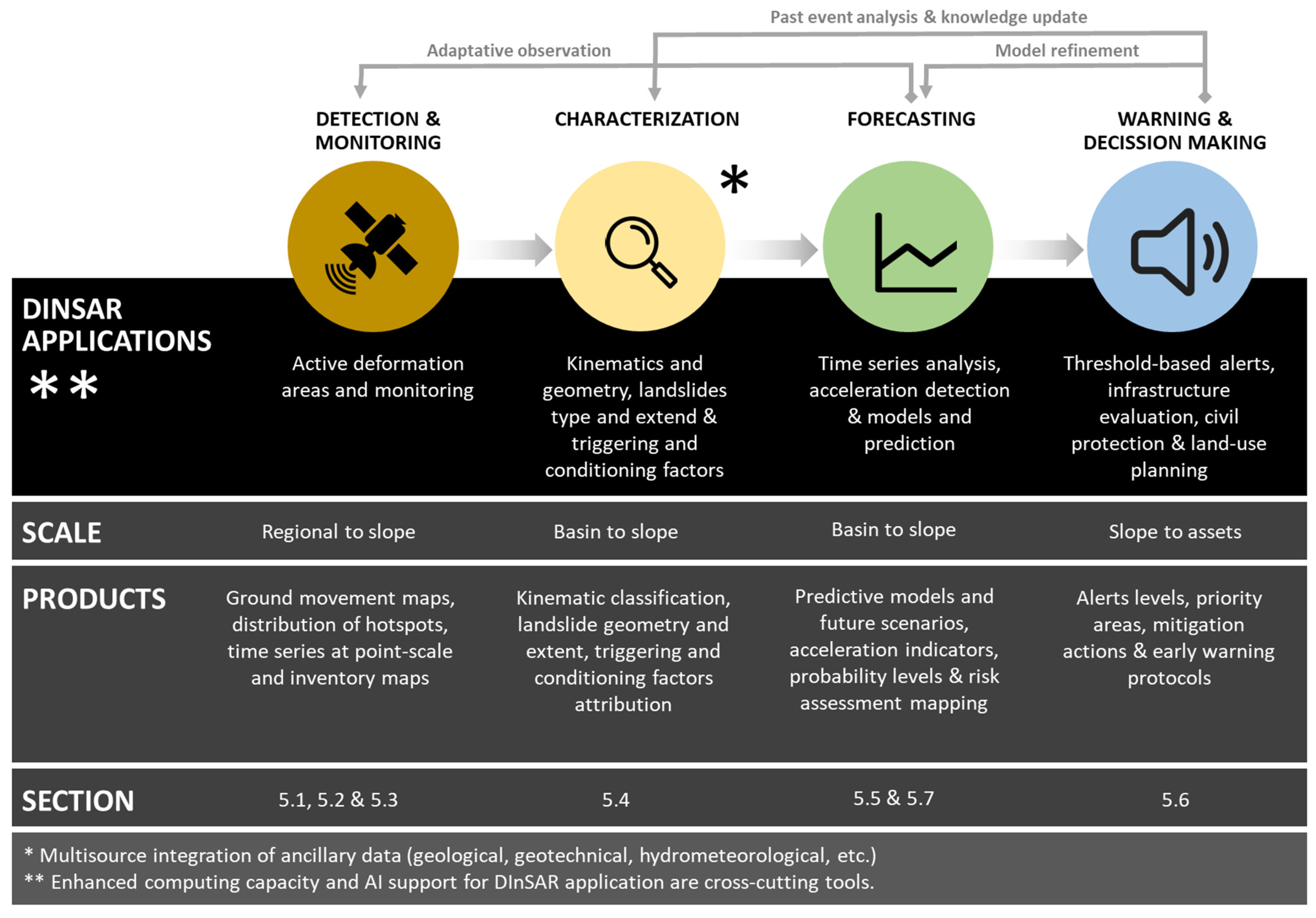
To synthesize the diverse roles of DInSAR in landslide studies and to clarify its contribution to operational risk management, Figure 2 presents a conceptual framework illustrating the progressive workflow from deformation detection to landslide characterization (mainly by integrating DInSAR data with multisource ancillary data), deformation forecasting, and support for warning and risk-informed decision-making, as well as the bidirectional flow between different InSAR applications. The framework emphasizes the transition from regional-scale deformation mapping to local, context-driven analyses, highlighting the main operational products and dominant working scales associated with each stage. It also highlights how artificial intelligence (AI) and enhanced computing capacities are becoming integral to all InSAR-landslide applications. The different applications shown in the figure are described in detail in this section.

5.1. Creation and Update of Landslide Inventories

One of the most remarkable features of DInSAR products is their broad spatial coverage combined with millimetric precision. This potential has been widely exploited for both the creation and the update of landslide inventories at different scales: local, e.g., [43], regional, e.g., [44], and national or continental, e.g., [45].

To generate new landslide inventories, displacement maps allow the identification of areas within the studied scene that exhibit movement and are thus active during the processed period. Subsequently, a process of delineation and classification of these active areas must be carried out. This process is complex, as some of the active areas identified through the DInSAR technique may be related to processes other than landslides, such as building settlement, karst processes, or ground subsidence.

Three main approaches can be found in the literature: (a) visual interpretation and expert-eased methods; (b) statistical methods; and (c) artificial intelligence methods. All these approaches can use either multi-temporal interferometric techniques or single-pair differential interferometry as input. The first method combines traditional methods with DInSAR products. It usually overlaps or projects MPs over DEMs and high-resolution optical images to identify and delineate landslides, for which expert supervision is required for detailed mapping and classification. The statistical and clustering methods enable the semi-automated extraction of geomorphological “objects” from massive InSAR datasets by identifying spatially significant deformation patterns. Techniques such as hotspot analysis (e.g., Getis-Ord Gi*) and unsupervised algorithms like Density-Based Spatial Clustering of Applications with Noise (DBSCAN) effectively group measurement points with similar displacement behaviors while filtering out background noise, e.g., [46,47,48]. Similarly, Active Deformation Areas (ADA) workflow transforms discrete data into coherent active landslide clusters based on predefined velocity thresholds and spatial density [49,50]. The last group of methods for mapping landslides from DInSAR data uses AI approaches to automate the generation of landslide inventories, e.g., [51,52].

When prior landslide inventories are available, the application of these techniques can provide not only the identification of new landslides but also the activity status of pre-existing landslides in the original inventory by comparing the activity state of the landslide in the inventory map and in the InSAR results [44,45,53]. This allows for establishing the activity status of inventoried landslides by comparing the existing inventory with the updated one.

While the aforementioned methods rely primarily on InSAR displacement time series, recent studies have shifted toward utilizing phase gradient measurements derived directly from interferograms. When integrated with artificial intelligence algorithms, these measurements enable the generation of high-accuracy landslide maps, particularly in complex mountainous terrains where traditional displacement analysis may face limitations, e.g., [51,54,55].

It is worth noting that, as in any other application of SAR interferometry, landslide mapping based on DInSAR can be affected by phase errors, which introduce uncertainties in the detection and the interpretation of measured movements. The most substantial contributor to phase noise is atmospheric phase delay, which can be divided into stratified delay (topographically correlated) and turbulent delay (associated with local water vapor variations). These errors can lead to false positives identified as landslides. However, they can be mitigated by applying external weather models [56] or auxiliary datasets [57] to subtract tropospheric delays in single interferograms, as well as by using spatio-temporal filters, specifically, high-pass filtering in time and low-pass filtering in space, exploiting the stochastic nature of the atmosphere, in the case of approaches based on time series. Furthermore, inaccuracies in the Digital Elevation Model (DEM) used for topographic phase removal result in phase residuals induced by the DEM. Additionally, uncertainties in precise orbit determination may create phase ramps across the interferograms. Although these ramps usually cover the whole interferogram, in some cases, they can be erroneously interpreted as landslide movements. Therefore, orbital errors must be corrected by re-estimating orbital parameters (e.g., using stable ground control points), while DEM errors must be corrected by estimating the residual topographic phase component. Finally, phase noise caused by temporal and spatial decorrelation can be minimized by the spatial averaging of measurement points (multilooking), while unwrapping errors should be addressed using robust algorithms that resolve phase ambiguity through spatial and temporal consistency [58]. In summary, fine processing techniques are required to mitigate these errors, especially to avoid the inclusion of false positives in DInSAR-derived landslide inventories.

5.2. Monitoring of Landslides

The temporal nature of DInSAR products allows for the spatiotemporal analysis of landslide evolution over extended periods. The technique provides displacement distributions in plane view (i.e., XY plane) for each available acquisition date, along with time–displacement series for all measurement points in the scene. This information makes it possible, among other things, to identify parts of the instability with higher velocities and periods of acceleration or deceleration, which are key data for risk management. DInSAR also provides time series (time–displacement plots) for each point, enabling the study of the evolution of individual or clusters of points, as well as the identification of trends and changes in displacement over time.

In the past, technical limitations, such as restricted storage, limited processing capacity, and long satellite revisit times, meant that DInSAR was primarily used as a mapping tool. This provided only a “snapshot” of the area of interest every few months or years, constituting a static approach. More recently, particularly following the launch of Sentinel-1 (with its 6 to 12-day revisit period) and the rise of cloud computing, DInSAR has evolved into a near-real-time monitoring system. This shift enables the detection of accelerations, decelerations, and seasonal fluctuations with high temporal resolution. Furthermore, the automatic ingestion and processing of newly acquired images facilitate the continuous monitoring and periodic updating of landslide activity. With such high spatial and temporal resolution, DInSAR can already be regarded as a robust and well-established technique for landslide monitoring. This is supported by broader evidence showing that DInSAR has evolved from a primarily experimental tool into a routine method for observing surface deformation in diverse phenomena, such as tectonic activity, volcanism, or anthropogenic processes [17]. Moreover, it has been widely adopted both as a standalone monitoring approach and as a key component in multi-technique frameworks, commonly with in situ geotechnical and geodetic methods or with optical remote sensing techniques, e.g., [59,60].

5.3. Retrospective Monitoring of Landslides

When a landslide occurs, it is often necessary to retrospectively study its recent displacement history prior to failure and its subsequent evolution to reconstruct the past. This information can be essential for understanding the triggering causes, supporting corrective stabilization measures, and even for legal and insurance applications to establish liabilities.

For this purpose, radar satellite images acquired before, during, and after the failure are analyzed. If the movement is very rapid, displacements during the failure event cannot be studied due to decorrelation between images. Therefore, processing is usually divided into different time periods, grouping SAR images before and after the failure, e.g., [61,62].

Extensive archives from ERS-1 (1991–2000), ERS-2 (1995–2011), ENVISAT (2002–2012), and Sentinel-1 (2014–present) satellites (C-band), as well as ALOS PALSAR (2006–2011) (L-band), are available for retrospective monitoring across most of the world over more than 30 years. SAR imagery from other satellites, such as TerraSAR-X (2007–present) and COSMO-SkyMed (2007–present), is also available for limited areas and can be used for retrospective processing.

5.4. Characterization

The DInSAR technique contributes significantly to the geomorphological characterization of landslides, complementing traditional analyses based on photointerpretation and fieldwork. It also helps establish causal relationships with different triggering factors, facilitating the identification of cause–effect dynamics.

5.4.1. Geomorphological Characterization

In terms of geomorphology, DInSAR helps define landslide boundaries (

Table 3. Geomorphological features of landslides that can be derived from DInSAR.

Geomorphological Features	Description	e.g., Ref.
Boundaries	DInSAR enables the determination of landslide boundaries, including perimeter, area, and shape. Other typical geomorphological parameters, such as the length and width of the displaced mass, can be derived from this information. Additional features, such as the total length, width, and length of the slip surface, require ancillary data to accurately delineate the landslide boundaries.	[63]
Typology	The type of landslide can be inferred by interpreting the spatial distribution of DInSAR-derived displacements within the landslide and by analyzing cross-sections of displacement along it (Figure 3). Complementary information is usually required to confirm the landslide type.	[63]
Sliding mass thickness	This parameter is calculated by inverting the DInSAR data. It requires establishing specific assumptions (e.g., that the surface displacement vector is parallel to the sliding surface), which may differ from reality in areas where significant thickening or thinning occurs. 3D displacements derived from DInSAR are used as input to calculate the sliding mass thickness (see Section 7).	[64,65]
Volume	The volume is inferred from the depth of the slip surface and the area of the landslide. It is usually determined at the pixel scale by summing the partial volumes obtained by multiplying the area of each pixel by the thickness of the landslide at that location.	[64]
Kinematics	The kinematics of landslides is usually determined by analyzing DInSAR time series. It enables the determination of the trajectory, velocity, and type of displacement trend. 2D decomposition of DInSAR displacements and 3D reconstruction using ancillary data (see Section 7 and Table 5) can significantly contribute to the evaluation of these features.	[66,67,68]
Internal partitioning	Landslides rarely move as a single block. DInSAR can be used to reveal landslide subunits by showing different velocity clusters or directions within the same slope.	[69,70,71]
Activity	DInSAR enables to determine the activity of landslides by providing high-precision displacement time series that allow for distinguishing between active, dormant, and reactivated states based on displacement variations.	[68,72]
Other	Although DInSAR does not directly detect geomorphological features such as tension cracks, scarps, or transverse ridges, detailed analysis of the magnitude, distribution and gradients in displacements can help guide their identification during fieldwork.

). Often, the sliding mass exhibits greater activity with clear displacement boundaries relative to the surrounding terrain, allowing precise delineation.

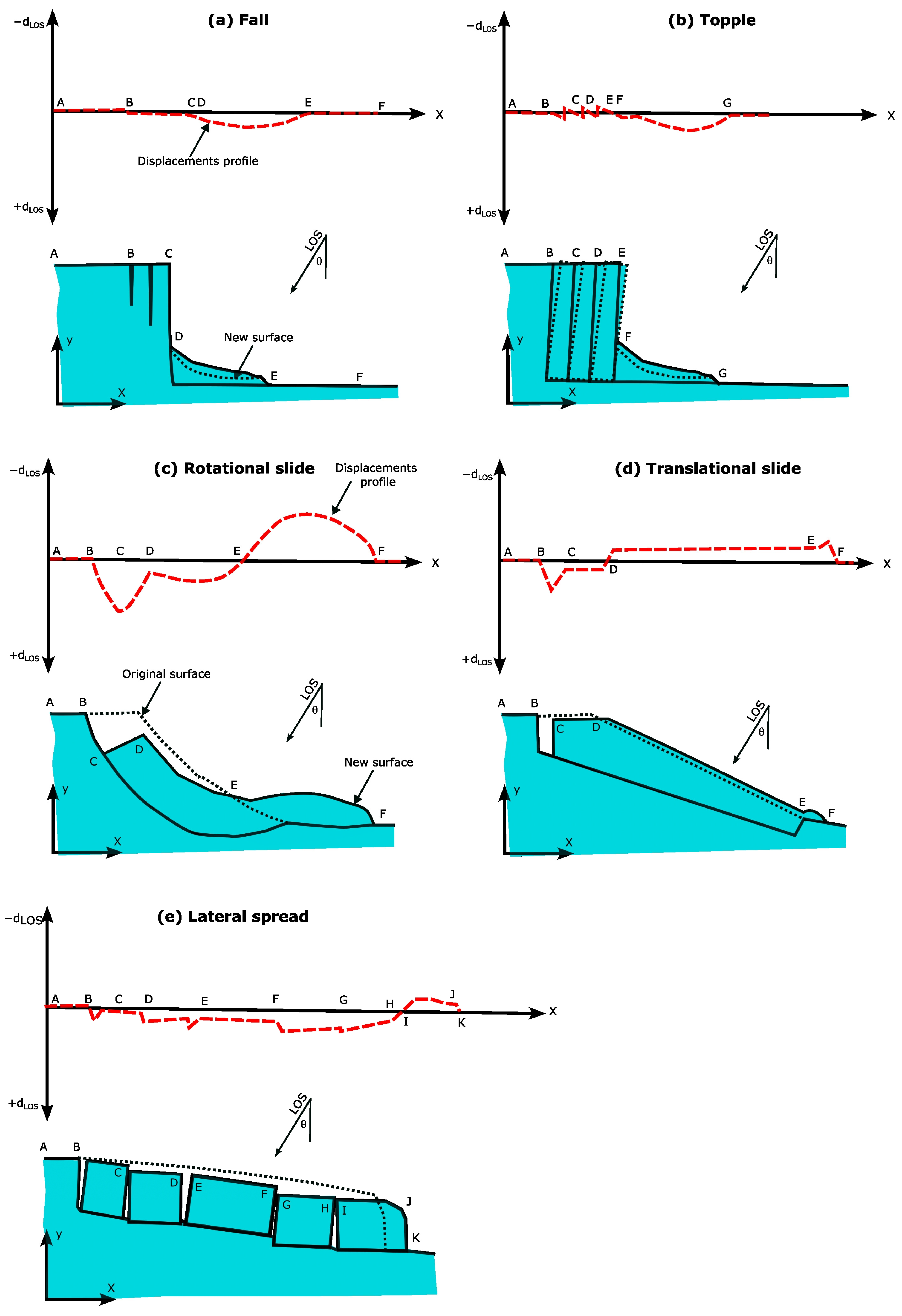
DInSAR also aids in interpreting the landslide type (Table 3). For example, in some rotational slides, uplift is observed in the toe area, while the head and body move downward. Some authors have studied deformation patterns of different landslide types in detail [63]. Figure 3 shows the theoretical longitudinal displacement profiles for different types of landslides, which could contribute to the identification of the landslide type.

Although DInSAR can independently provide decisive information for geomorphological characterization, it is primarily a diagnostic tool for detecting active areas of landslides. These areas often correspond to smaller movements within larger landslides, which can lead to an underestimation of their overall dimensions and potential hazard. For this reason, DInSAR should always be integrated with historical, geological, geotechnical, climatological, and other types of data for a correct characterization and mapping of landslides.

The slip surface, kinematics, activity and volume of landslides are relevant parameters for their geomorphological characterization, which can be derived from DInSAR (Table 3). For example, Frattini, Crosta, Rossini and Allievi [68] proposed a method based on PS-DInSAR data that served to assess the kinematic behavior of landslides (particularly deep-seated ones) and provided insights into the shape and depth of the slip surface. More recently, Chen, Li, Song, Yu, Tomás, Du, Li, Mugabushaka, Zhu and Peng [64] proposed a methodology to derive the slip surface and volume of landslides from DInSAR datasets by inverting quasi-3D DInSAR displacements.

Given that DInSAR only captures surface-level movements, integrating it with in situ data, such as inclinometers or geophysical surveys, is essential. This multisource approach validates subsurface geomorphological features inferred from surface displacements, thereby reducing uncertainty and ensuring a more comprehensive characterization of landslide dynamics.

5.4.2. Identification and Characterization of Triggering Factors

By comparing DInSAR time series or maps with potential triggers such as earthquakes [73], rainfall [74], piezometric levels [75], reservoir water levels [76] or cryospheric processes such as freeze–thaw cycles [77], causal relationships can be identified. These improve our understanding of instability mechanisms, help define more effective mitigation measures, and enhance modeling efforts.

These relationships can be established qualitatively through direct comparison of time series or maps. The simplest approach is to compute direct correlations between DInSAR data and the triggering factors. This correlation provides a straightforward relationship between displacements and a single factor, typically expressed as a correlation coefficient. However, these simple analyses fail to account for the non-linear nature of the relationship or the temporal lag often observed between the trigger and the displacement. For instance, peak deformation may occur significantly after a rainfall event due to the slow infiltration of water and the subsequent rise in pore-water pressure.

Consequently, advanced signal decomposition and correlation methods have emerged. Wavelet tools (e.g., cross wavelet transform and wavelet coherence) are now widely used to quantify the non-stationary relationship and specific time lags between triggers (e.g., intense rain) and DInSAR displacement responses [78]. However, the results are highly sensitive to the choice of the mother wavelet. Gray relational analyses quantify the degree of geometrical similarity between DInSAR displacement series and potential triggers [79]. This method requires equidistant data points in both time series and does not account for physical time lags.

Other decomposition methods, such as Principal Component Analysis (PCA) [80], Independent Component Analysis (ICA) [81], and Seasonal-Trend decomposition using Locally Estimated Scatterplot Smoothing (STL-LOESS) [82], effectively isolate seasonal signals from long-term gravitational trends. Specifically, PCA enables the identification of dominant regional patterns and the reduction of data dimensionality. However, its decomposition is constrained by orthogonal components that maximize variance, which do not always represent independent physical processes. In contrast, ICA facilitates the unsupervised separation of linearly mixed signal sources; nevertheless, it cannot perfectly separate Gaussian-distributed sources, and its computational cost is higher than that of PCA. Finally, STL-LOESS decomposition separates time series, without considering the spatial location of the points, into trend, seasonal, and residual components, providing robustness against outliers, but it is highly sensitive to the choice of smoothing window, which must be carefully selected to avoid signal loss.

More recently, AI, explainable AI and hybrid methods have been used to identify the most relevant triggering factors and recognize the complex coupling between external triggers and landslide motion, e.g., [83]. Ensemble methods such as Random Forest (RF) and eXtreme Gradient Boosting (XGBoost) are widely employed to rank the relative importance of conditioning factors of landslides, e.g., [84]. SHAP (SHapley Additive exPlanations) values are applied to these models to interpret the non-linear contribution and direction of each triggering or conditioning factor, e.g., [67]. Furthermore, Deep Learning architectures, particularly Long Short-Term Memory (LSTM) networks and Attention Mechanisms, are essential in uncovering complex temporal dependencies, allowing researchers to pinpoint critical lag times and seasonal windows where specific factors exert the greatest influence on landslide kinematics.

These methods help identify the main triggering factors, seasonal components, time lags between triggering factors and displacements, and different deformation components within each time series that correlate more directly with triggering factors.

5.5. Mapping of Susceptibility, Hazard, Vulnerability, and Risk

While DInSAR does not measure risk directly, it informs key risk components. However, its integration into comprehensive risk mapping remains challenging and requires complementary data and methods. DInSAR data has been successfully used to develop exposure, susceptibility, hazard, vulnerability, and risk maps, e.g., [85].

Traditional susceptibility mapping can be enhanced by DInSAR, as it provides data on active or incipient slope movements that are often difficult to identify through geomorphological mapping alone. DInSAR information from landslide-affected areas (active points or areas) can be combined with conditioning factors to develop or refine susceptibility maps, e.g., [82,86]. In essence, overlaying DInSAR-derived displacement data, represented as points or polygons, with spatial layers of conditioning factors enables statistical methods (e.g., logistic regression, weight of evidence, or analytical hierarchy process) and machine learning algorithms (e.g., Random Forest, XGBoost, or Support Vector Machines) to identify correlations with past or ongoing movements, e.g., [87,88,89]. These correlations are subsequently used to generate susceptibility maps that highlight areas with a higher probability of landslide occurrence.

Landslide hazard mapping incorporates the temporal probability of occurrence and, in some cases, the expected magnitude of landslides. Therefore, DInSAR can be used for hazard assessment by enabling the analysis of ground deformation time series and kinematic evolution of unstable slopes, e.g., [90].

Vulnerability mapping focuses on evaluating the potential for exposed elements to be damaged by a landslide. Consequently, vulnerability cannot be directly measured by DInSAR, as it depends on other factors (e.g., structural, social, or economic). However, DInSAR can indirectly contribute by identifying elements exposed to deformations, which can, in turn, be used to assess potential damage [91]. Furthermore, when combined with ancillary data (e.g., building typology or construction materials), DInSAR can be used to identify and zone vulnerable elements, for instance, through the calibration of fragility curves relating DInSAR displacements or displacement rates to levels of damage, e.g., [92].

Finally, landslide risk mapping integrates the aforementioned variables to estimate potential losses or costs. Various approaches can be employed by combining one or more DInSAR-derived variables. Artificial intelligence techniques have also been used to assess landslide risk, e.g., [93,94].

In summary, DInSAR data are primarily used to create or enhance the landslide inventories that form the basis of the susceptibility analysis, evaluate hazard through the provided temporal information, assess the vulnerability of exposed elements, or evaluate risk through the integration of the aforementioned variables, as well as to validate the resulting maps.

5.6. Evaluation of the Impact of Landslides on Assets or Infrastructure

Combining DInSAR data with asset or infrastructure maps allows the identification of critical situations and the assessment of landslide impacts, as well as providing essential information for prioritizing maintenance and reinforcement efforts. In urban areas, where coherence is high, measurement points are mostly located on buildings and infrastructure. Consequently, measured displacements typically correspond to these structures, facilitating the assessment of landslide impact on them.

Although some studies use C-band data, high-resolution satellites such as TerraSAR-X, PAZ, and CosmoSkyMed (X-band) provide better spatial resolution, often detecting multiple MPs on a single structure [95]. This enables a more detailed and thorough analysis of individual assets or infrastructure.

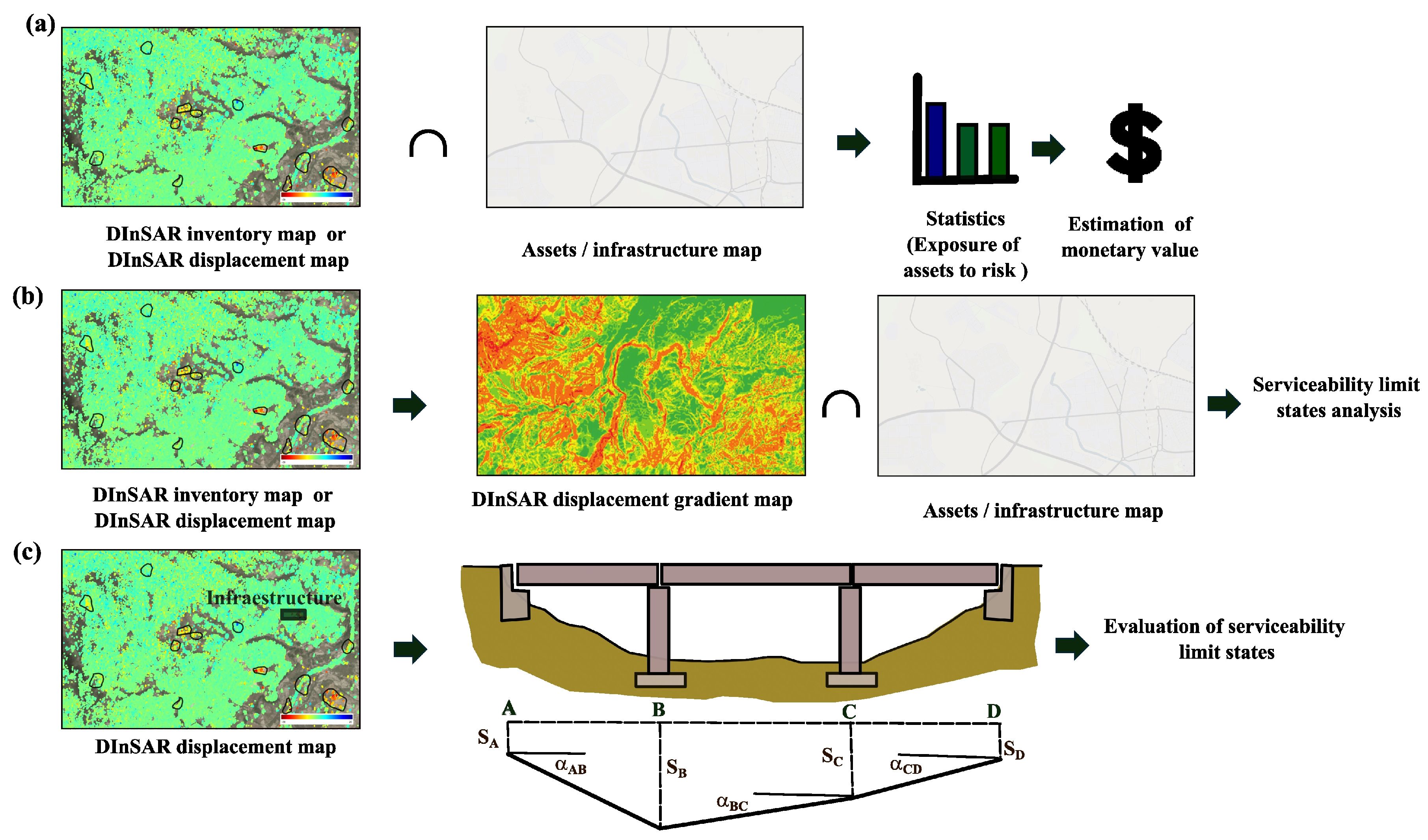
The simplest analysis corresponds to the evaluation of the exposure of assets or infrastructure to landslides. This analysis is performed by determining which and how many assets or infrastructure are located in active landslide zones detected by DInSAR. To this aim, DInSAR displacement maps are intersected with cadastral or infrastructure maps (Figure 4a). This helps identify potentially affected assets or infrastructure and supports cost-based exposure statistics [96].

Another analysis involves interpolating DInSAR data to detect deformation “anomalies”. These are generally defined in terms of gradients calculated from MPs on infrastructure or assets, e.g., [97], and are performed at a regional scale (Figure 4b). Those areas exhibiting high deformation gradients present important uneven displacements that can affect infrastructure and assets, e.g., [91].

Detailed analysis of affected infrastructure can also be conducted using MPs on the structures, assuming they reflect ground movement (Figure 4c). Construction codes define serviceability limits (e.g., angular distortion, maximum vertical and horizontal displacements), allowing evaluation of damage levels.

A specific application developed by Del Soldato, Solari, Poggi, Raspini, Tomás, Fanti and Casagli [92] involved creating empirical fragility curves for buildings on a landslide using DInSAR data combined with a damage inventory. These curves were then used to estimate the probability of building damage based on a new DInSAR displacement map.

Finally, DInSAR has been employed to evaluate the effectiveness of mitigation strategies by comparing landslide activity levels before and after the implementation of stabilization measures, e.g., [97,98].

Although all the approaches described above aim to identify critical situations and evaluate the state of buildings and infrastructure, DInSAR can also be used as a preventive tool in land management. It supports urban development strategies by detecting areas with potential instabilities that should be designated as unsuitable for development.

5.7. Contribution to Landslide Model Development

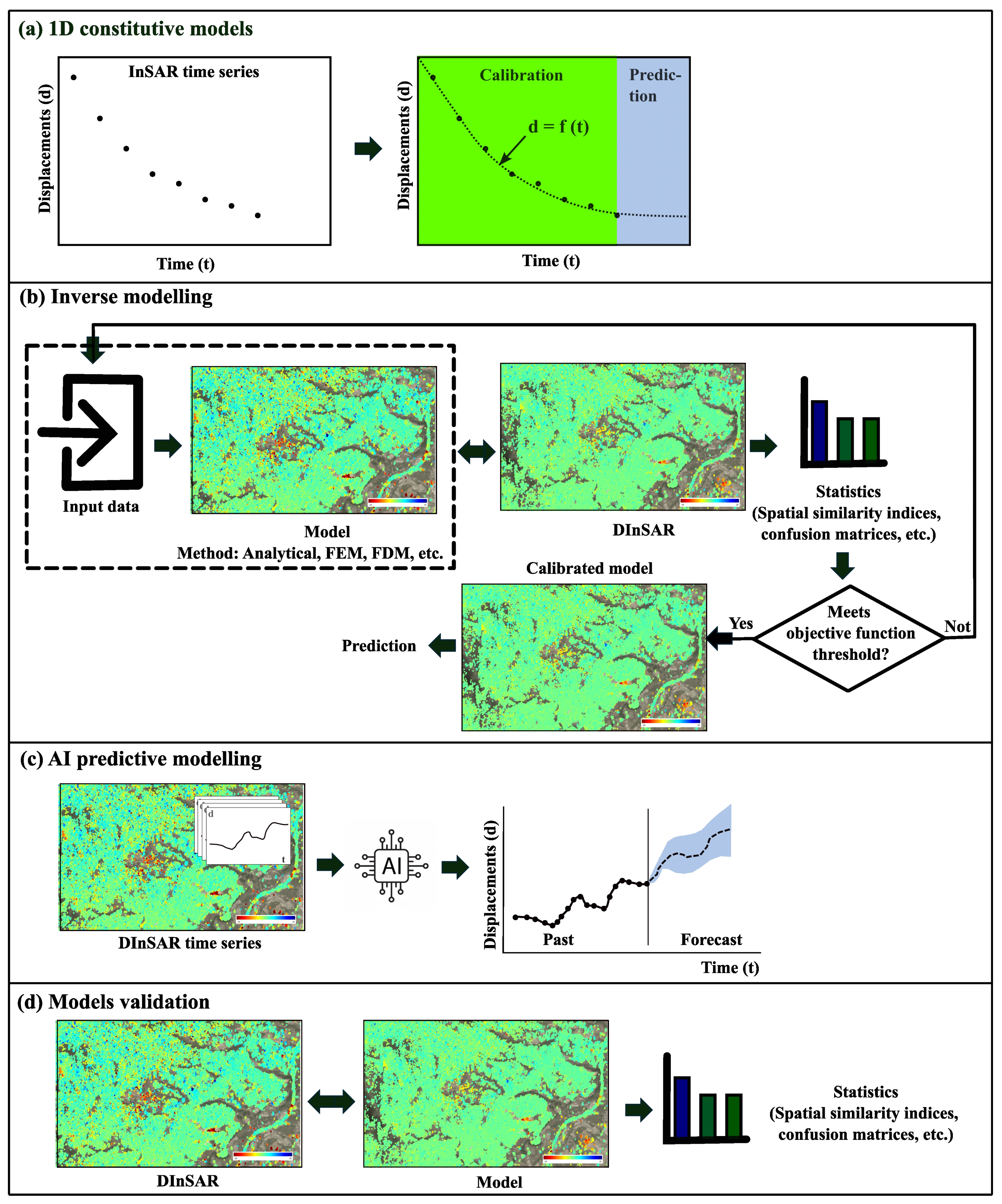
DInSAR data plays a key role in landslide modeling, providing a fundamental basis for parameter calibration, model optimization, and result validation. Specifically, a first application involves using DInSAR time series to calibrate one-dimensional constitutive models capable of replicating certain landslide deformation phases, e.g., [99]. This application basically consists of fitting functions physically representing the landslide movement to the DInSAR time series (Figure 5a). There are well-known analytical models that can fit very well the different phases of creep behavior of landslides.

Another approach involves determining terrain parameters via inverse modeling by minimizing differences between observed and modeled displacements, e.g., [12,100,101]. This is generally framed as an optimization problem [102]. In this approach, initial input parameters are selected to compute a model. The model is then compared with DInSAR data to assess their similarity from a statistical point of view (Figure 5b). To this end, an objective function is defined. If the model does not meet the defined threshold for the objective function, the input parameters are adjusted to compute a new model. This iterative process is repeated until the differences between the model and the DInSAR data fall below the predefined threshold, thereby reducing the uncertainty of geotechnical properties in complex landslide systems. The resulting model is then accepted and can be used to predict future scenarios.

Artificial intelligence predictive models analyze historical and real-time InSAR displacement datasets to forecast future trends (Figure 5c). These methods are also becoming highly popular and are being extensively used as prediction tools to determine the evolution of landslide displacements over time, e.g., [103,104].

Finally, DInSAR data are widely used to validate numerical models by comparing observed displacements with model outputs to statistically or qualitatively assess their accuracy (Figure 5d). This approach ensures that the model accurately captures both the temporal evolution and the spatial boundaries of the landslide mass.

6. Detection Capability of the DInSAR Technique According to Landslide Types

As previously discussed, the detection capacity of DInSAR essentially depends on the level of backscatter from the landslide surface, the movement velocity and the size of the landslide. Regarding backscatter, landslides that develop in rock generally exhibit higher backscatter than those in soil. Additionally, vegetation presence contributes to decorrelation.

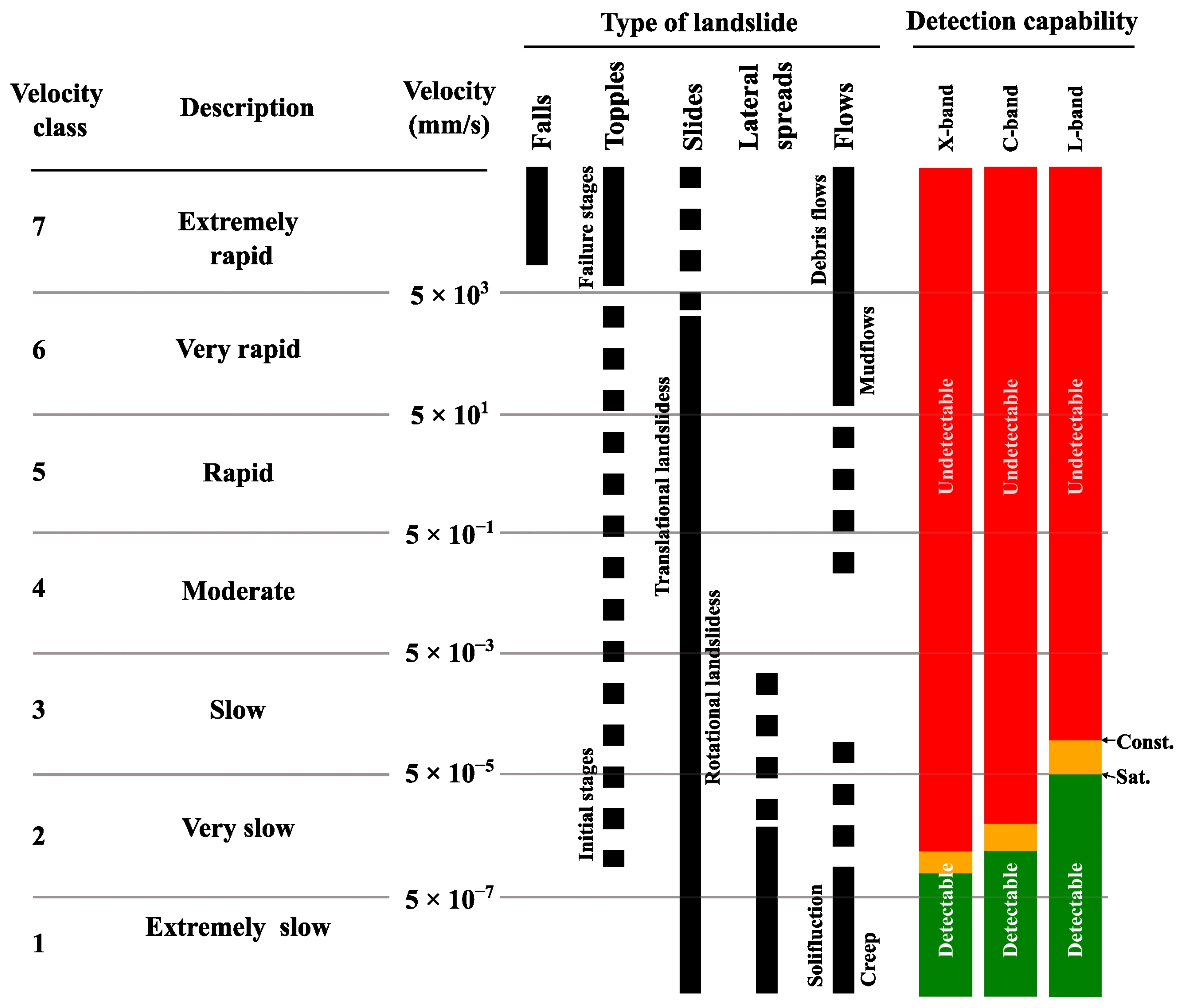
As for velocity, space-borne DInSAR is able to detect “Extremely slow” and “Very slow” landslides (see Section 3), according to the Cruden and Varnes [41] classification (Figure 6). Furthermore, ‘Slow’ movements can be partially detected when a satellite constellation reduces the revisit time, thereby increasing the maximum detectable displacement threshold (Figure 6).

Falls, topples, and some types of flows tend to occur rapidly (from meters per month to meters per second, i.e., “Moderate” to “Extremely rapid” landslides according to the Cruden and Varnes [41] classification), which generally makes their detection using DInSAR impossible due to decorrelation effects. However, DInSAR can still be used to identify precursor movements, as well as post-failure processes associated with these types of landslides, such as secondary landslides and the consolidation of debris deposits, e.g., [105,106].

In contrast, DInSAR is well-suited to detect “Extremely slow” to “Very slow” movements (from a few mm/year up to several cm/year, according to the Cruden and Varnes [41] classification) typically associated with slides, lateral spreads, and specific flows such as solifluction, which fall within the sensitivity range of the technique (see Section 3).

Although in some cases, rotational and translational slides may experience sudden failures and reach high velocities, these often exhibit “Extremely slow” or “Slow” velocities, making them detectable through DInSAR, e.g., [82,107,108]. Precursor deformations can also be detected by DInSAR in these types of landslides.

Lateral spreads are characterized by very low velocities, usually “Extremely slow”. While this makes them detectable by DInSAR, in some cases, the movement falls within the error range, making it difficult to distinguish displacement from noise and challenging to monitor them with this technique.

Flows can present different kinematic characteristics. Debris flows cannot be detected by DInSAR due to their high velocity (i.e., up to tens of meters per second) and the geometrical changes occurred in the mobilized mass, that causes decorrelation. However, after deposition, the debris flow deposits consolidate, making them detectable by DInSAR. Other flow types such as solifluction present very low velocities and clear seasonal deformation patterns correlated to freeze–thaw cycles [77]. Finally, earth flows can exhibit different velocities. Only those earthflows exhibiting “Extremely slow” or “Slow” velocities can be monitored by DInSAR.

The minimum detectable size of a landslide is intrinsically linked to the wavelength band, as discussed in Section 3. X-band sensors are capable of resolving features down to a small-scale, whereas the detection threshold for C-band is limited to small-to-medium-sized landslides. In contrast, L-band sensors are generally restricted to the identification of medium-scale or larger mass movements.

Figure 6. Landslide velocity classification based on [41,109] showing the relationship between landslide types, velocity classes, and the detection capabilities of X-, C-, and L-band DInSAR sensors. The green areas indicate the detectable velocity range for individual satellites (Sat.), while the orange areas delimit the extended range achieved by using a satellite constellation (Const.) for each frequency band. Red areas represent the velocities ranges that are undetectable by DInSAR.

Figure 6. Landslide velocity classification based on [41,109] showing the relationship between landslide types, velocity classes, and the detection capabilities of X-, C-, and L-band DInSAR sensors. The green areas indicate the detectable velocity range for individual satellites (Sat.), while the orange areas delimit the extended range achieved by using a satellite constellation (Const.) for each frequency band. Red areas represent the velocities ranges that are undetectable by DInSAR.

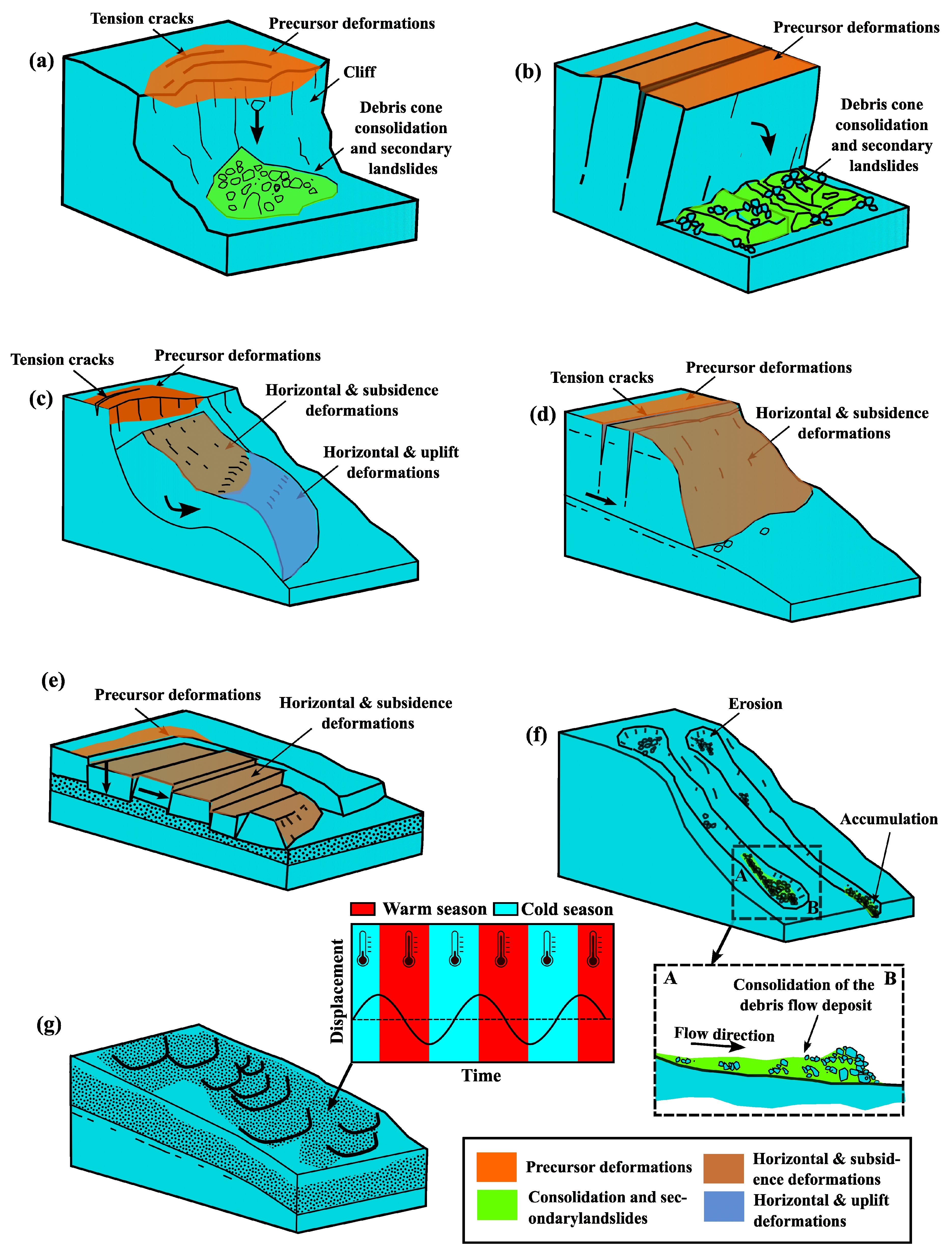
Table 4 summarizes the detection and monitoring capacity of DInSAR for different types of landslides shown in Figure 7.

Figure 7. Main features potentially detected by DInSAR in different types of landslides: (a) falls; (b) topples; (c) rotational slide; (d) translational slide; (e) lateral spread; (f) debris flow; and (g) solifluxion. See Table 4 for a detailed description of the detection and monitoring capabilities of DInSAR. A–B in subfigure (f) represents a cross-section along the debris flow channel.

Figure 7. Main features potentially detected by DInSAR in different types of landslides: (a) falls; (b) topples; (c) rotational slide; (d) translational slide; (e) lateral spread; (f) debris flow; and (g) solifluxion. See Table 4 for a detailed description of the detection and monitoring capabilities of DInSAR. A–B in subfigure (f) represents a cross-section along the debris flow channel.

Table 4. Detection and monitoring capability of various landslide types using DInSAR.

Type	Detection and Monitoring Capacity Using DInSAR
Falls (Figure 7a)	Typically, small size and very fast movements that cannot be detected by DInSAR. They often occur on steep slopes, leading to geometric distortions in the images. Only precursor displacements can be detected, generally limited to the crest of the slope and colluvial deposits. After the event, decorrelation occurs. Consolidation and secondary landslides of the debris cone deposits can also be detected.
Topples (Figure 7b)	Typically, small–medium size, very fast and undetectable by DInSAR. However, some slopes affected by toppling show slower velocities, allowing for detection and monitoring before collapse. Like falls, precursors and post-failure movements of colluvial deposits can sometimes be identified. Detection is usually limited to the slope crest. Consolidation and secondary landslides of the debris cone deposits can also be detected.
Slides (Figure 7c,d)	DInSAR can successfully detect and monitor “extremely slow” and, to some extent, “very slow” landslides. The main limitation regarding size is the detection of very small landslides. It can also detect precursor deformations of faster slides. Rotational slides often show uplift in the toe area and subsidence at the head. Precursors’ movements on the crown of the landslides can also be detected.
Lateral spreads (Figure 7e)	These movements tend to be very slow, making them detectable and monitorable by DInSAR. In some cases, movements are so slow that they approach the technique’s detection threshold. Typically characterized by large dimensions that facilitate their detection.
Flows (Figure 7f,g)	Fast flows (e.g., debris, mud, and some earth flows) cannot be detected due to their high speed, narrow width and internal decorrelation. Only the consolidation of the debris flow deposits can be detected. However, “extremely slow” or “slow” earth flows (e.g., solifluction) and creep can be studied using DInSAR. Solifluction exhibits a seasonal pattern in the time series.

Table 4. Detection and monitoring capability of various landslide types using DInSAR.

Type	Detection and Monitoring Capacity Using DInSAR
Falls (Figure 7a)	Typically, small size and very fast movements that cannot be detected by DInSAR. They often occur on steep slopes, leading to geometric distortions in the images. Only precursor displacements can be detected, generally limited to the crest of the slope and colluvial deposits. After the event, decorrelation occurs. Consolidation and secondary landslides of the debris cone deposits can also be detected.
Topples (Figure 7b)	Typically, small–medium size, very fast and undetectable by DInSAR. However, some slopes affected by toppling show slower velocities, allowing for detection and monitoring before collapse. Like falls, precursors and post-failure movements of colluvial deposits can sometimes be identified. Detection is usually limited to the slope crest. Consolidation and secondary landslides of the debris cone deposits can also be detected.
Slides (Figure 7c,d)	DInSAR can successfully detect and monitor “extremely slow” and, to some extent, “very slow” landslides. The main limitation regarding size is the detection of very small landslides. It can also detect precursor deformations of faster slides. Rotational slides often show uplift in the toe area and subsidence at the head. Precursors’ movements on the crown of the landslides can also be detected.
Lateral spreads (Figure 7e)	These movements tend to be very slow, making them detectable and monitorable by DInSAR. In some cases, movements are so slow that they approach the technique’s detection threshold. Typically characterized by large dimensions that facilitate their detection.
Flows (Figure 7f,g)	Fast flows (e.g., debris, mud, and some earth flows) cannot be detected due to their high speed, narrow width and internal decorrelation. Only the consolidation of the debris flow deposits can be detected. However, “extremely slow” or “slow” earth flows (e.g., solifluction) and creep can be studied using DInSAR. Solifluction exhibits a seasonal pattern in the time series.

7. Emerging Challenges and Future Directions

Today, DInSAR constitutes a fundamental technique for studying landslides, but its application still faces challenges that, despite recent advances, require further attention in the future. Below is a review of the most notable recent developments and upcoming challenges.

One major limitation is the inability to measure north–south displacements due to the SAR image acquisition geometry. In landslides exhibiting a predominant E-W displacement component, the N-S displacement can be neglected when reconstructing the 3D components of movement. However, this assumption is not valid for landslides that exhibit significant N-S movement components. Nevertheless, under specific assumptions—such as planar motion or movement parallel to the terrain surface—it is possible to estimate the three displacement components, e.g., [99]. This method is highly dependent on the DEM quality and assumes a direction of movement that does not always reflect the physical reality of the landslide (Table 5). Moreover, combining DInSAR data from ascending and descending tracks with external data (e.g., photogrammetry, offset-tracking or Global Navigation Satellite Systems (GNSS)) allows for the reconstruction of the full 3D displacement field of a landslide, e.g., [82] (Table 5). This approach improves accuracy and sensitivity to horizontal movements but requires multiple well-aligned datasets and involves higher processing complexity, potential error propagation, and greater computational and operational costs. Multi-pass DInSAR can also be used to estimate 3D displacements with high accuracy by combining right- and left-looking datasets (e.g., from COSMO-SkyMed and RADARSAT-2) [110]. More recently, the use of NewSpace SAR constellations with inclined orbits has opened the door to the high-accuracy reconstruction of 3D landslide displacements with increased revisit frequency, e.g., [111]. However, these satellites are not intended for operational monitoring purposes because the acquisitions are taken on demand, not as part of standard acquisition plans with a scheduled revisit time and large-scale coverage. Regarding the limitations related to the geometry of observation, recent advances with drones mounting SAR sensors have demonstrated an excellent performance in dedicated experiments for 3D displacement retrieval over complex scenarios with daily revisit [112].

The use of BIM (Building Information Modeling) and Digital Twins is emerging as a powerful tool in engineering practice and more specifically in the field of landslides, e.g., [113,114,115]. The integration of DInSAR data into Building Information Modeling (BIM) environments allows for the precise mapping of surface displacements onto specific structural components, facilitating the structural health monitoring of vulnerable infrastructure impacted by landslides. Complementarily, Digital Twins couple these BIM geometries with physics-driven numerical models and remote sensing data. This evolution enables the development of long-term predictive simulations, determination of parameters by inversion, and the assessment of how landslides impact the stability of mitigation structures. The integration of DInSAR into these frameworks is not merely a visual overlay but a structural data ingestion. Therefore, DInSAR acts as a functional data input that feeds BIM structural alerts and provides Digital Twins with physical constraints for predictive modeling. Although the number of applications involving DInSAR as input of BIM or Digital Twins for landslides, or the infrastructure they affect, is limited in the scientific literature, several successful case studies have been reported. D’Amico et al. [116] developed a BIM model for road infrastructure management that integrates ground-penetrating radar, mobile laser scanning, and DInSAR data to assess pavement conditions. Another notable example is the Digital Twin of the Alps [117], part of ESA’s Regional Initiative 3 [118], which includes landslide simulation and aims to support decision-making in natural and environmental risk mitigation.

Thanks to the short revisit intervals of SAR satellites, large image collections can be acquired in short periods, allowing for regular DInSAR processing updates and identification of anomalous landslide behavior. Analyzing MPs’ time series enables the detection of critical pre-failure conditions, commonly using traditional inverse velocity methods to estimate the time of failure. In recent years, this approach has shown success in retrospective landslide predictions, e.g., [119,120,121]. However, most of these analyses are post-event. Consequently, establishing a quasi-real-time early warning system based on InSAR data remains challenging. Even though processing times can be optimized, automated, and considerably reduced, the revisit period (typically 6–12 days) and data availability (ranging from a few hours during emergencies to 1–2 days in standard operations) strongly condition the response time of early warning systems. These constraints often prevent the timely detection of rapid, catastrophic failures, where the acceleration phase typically occurs between two consecutive acquisitions. Another source of delay is the analysis, interpretation, decision-making and dissemination of results to authorities, who must make decisions based on the generated products. These stages may require a short amount of time (from a few minutes to a few hours) and can also be automated, although they usually require expert supervision. Furthermore, results can be affected by atmospheric artifacts or phase unwrapping errors (see Section 5.1), which may lead to false alarms and hinder the implementation of automated alert systems.

Table 5. Summary of methods to estimate 3D displacement from DInSAR datasets. Adapted from [110].

Method	Advantages	Disadvantages
Negligible N-S motion	Simple. Only requires ascending and descending datasets.	Only valid when the movement is purely E-W.
Multi-pass D-InSAR by combining right- and left-looking datasets	Simple. Provides high accuracy for all three displacement components	Reduced performance at high latitudes due to limited viewing geometry diversity. Scarcity of SAR platforms with left-looking acquisition capabilities.
Surface-parallel motion	Only requires ascending and descending datasets. High accuracy for horizontal components.	Assumes a direction of movement that does not always reflect the physical reality of the landslide, which can introduce significant errors, especially in cases of complex motion or when the terrain is poorly represented by the DEM.
Multi-sensor 3D displacement estimation (combination of DInSAR and GNSS, or offset tracking, or other techniques)	Improves accuracy and reliability. Quite sensitive to horizontal movements.	Requires multiple datasets, which may not always be available or well-aligned in space/time. Increased complexity in processing. There is error propagation between sources. Presents a higher computational and operational cost.
NewSpace SAR constellations with inclined orbits	Non-polar orbit acquisitions. High-accuracy 3D displacement estimation. Higher revisit frequency.	Less orbital accuracy. More complex processing. On-demand acquisition plans and small spatial coverage.

Table 5. Summary of methods to estimate 3D displacement from DInSAR datasets. Adapted from [110].

Method	Advantages	Disadvantages
Negligible N-S motion	Simple. Only requires ascending and descending datasets.	Only valid when the movement is purely E-W.
Multi-pass D-InSAR by combining right- and left-looking datasets	Simple. Provides high accuracy for all three displacement components	Reduced performance at high latitudes due to limited viewing geometry diversity. Scarcity of SAR platforms with left-looking acquisition capabilities.
Surface-parallel motion	Only requires ascending and descending datasets. High accuracy for horizontal components.	Assumes a direction of movement that does not always reflect the physical reality of the landslide, which can introduce significant errors, especially in cases of complex motion or when the terrain is poorly represented by the DEM.
Multi-sensor 3D displacement estimation (combination of DInSAR and GNSS, or offset tracking, or other techniques)	Improves accuracy and reliability. Quite sensitive to horizontal movements.	Requires multiple datasets, which may not always be available or well-aligned in space/time. Increased complexity in processing. There is error propagation between sources. Presents a higher computational and operational cost.
NewSpace SAR constellations with inclined orbits	Non-polar orbit acquisitions. High-accuracy 3D displacement estimation. Higher revisit frequency.	Less orbital accuracy. More complex processing. On-demand acquisition plans and small spatial coverage.

Consequently, from an operational perspective, the implementation of a quasi-real-time early warning system based on DInSAR data involves a sequence of steps [119,122]: (i) data acquisition; (ii) data processing; (iii) analysis and interpretation; (iv) decision-making; and (v) communication of warnings to the public. Each of these steps introduces a delay that conditions the overall response time of the system, typically extending it from 7 to 14 days. Therefore, reducing revisit periods, minimizing acquisition, processing, analysis, and decision-making times, and establishing structured protocols are necessary for DInSAR to function as a near-real-time early warning system. In this regard, the use of the aforementioned NewSpace SAR constellations can significantly contribute to reducing these timeframes.

It should be noted, however, that while in situ sensors (e.g., inclinometers or extensometers) provide local point measurements with high temporal resolution, spaceborne DInSAR offers wide spatial coverage with more limited temporal revisit. The integration of both techniques addresses their respective limitations, providing a robust framework for operational early warning systems [119]. Ultimately, it can be concluded that, at present, DInSAR is not competitive on its own as a real-time early warning system when compared to continuous monitoring techniques.

Enhanced computing capacity, driven by parallelization, optimized algorithms, and cloud computing, has significantly increased the efficiency and frequency of large-scale DInSAR updates, e.g., [123]. A practical example is the methodology implemented in Tuscany (Italy), where Sentinel-1 images are processed continuously, updating displacement data every 6 to 12 days as new acquisitions become available, to detect emerging instabilities and monitor existing ones [124]. This approach has enhanced early detection of deformational anomalies and improved risk management at the regional levels.

Another consequence of enhanced computing capabilities, combined with the increasing availability of open-access, high-revisit imagery (e.g., from the Sentinel constellation), is the development of services of DInSAR datasets processed at country or continental scales such as the European Ground Motion Service (EGMS) and the Observational Products for End-Users from Remote Sensing Analysis (OPERA), both of which utilize a hybrid PS and DS approach. EGMS provides LOS (basic and calibrated, using a geodetic referencing process) and ortho (vertical and east–west) displacement data across Europe since 2015, accessible through an online visualization platform [125]. The data can be downloaded in different formats using the EGMS portal and present a mean velocity standard deviation of 0.7 mm/yr [126]. In addition, a dedicated application has been developed by Becattini et al. [127] to store, customize, and convert EGMS ground motion data into geospatial databases, either burst by burst or for an area of interest. Similarly, OPERA provides InSAR products covering North America with a 30 m spatial resolution, a millimeter-level precision, and a temporal frequency of 12 days by integrating Sentinel-1 (C-band) and NISAR (L-band) data from September 2016 [128]. The use of L-band images by OPERA notably increases coherence in vegetated North American terrains, overcoming the temporal decorrelation that hinders landslide monitoring in these regions. Additionally, countries such as Norway [129], the Netherlands [130] and Germany [131] have performed their own country-wide InSAR processing.

In the last decade, the number of SAR satellites has increased significantly (e.g., PAZ and LuTan-1), and new missions are planned (e.g., NISAR and ROSE-L), which will enhance spatial and temporal coverage [132,133,134]. These advancements further facilitate DInSAR applications in landslide research, providing different detection capabilities through the use of different frequency bands, incidence angles, sensor look directions and spatial resolutions, among other technical specifications. Additionally, the increase in the number of SAR satellites, combined with higher observation frequency, brings us closer to quasi-real-time monitoring of landslide movements.

Among all emerging advancements in the use of InSAR for landslide research, artificial intelligence is clearly the most significant. AI is becoming increasingly relevant for DInSAR data interpretation, prediction, and risk assessment in the field of landslides. These techniques could facilitate the management and automatic analysis of the large amounts of data generated by DInSAR, maximizing its benefits [17]. In line with the applications outlined in earlier sections, numerous recent studies have integrated AI with DInSAR datasets to develop susceptibility and hazard maps, identify and map landslide boundaries, predict time series behavior, detect critical phases, define rainfall thresholds, and integrate multi-source data, among other emerging applications, e.g., [135,136]. However, the success of AI within the field of DInSAR for landslide research strongly depends on model transparency, spatial transferability, and data efficiency, e.g., [137,138,139]. In terms of interpretability, some models are inherently opaque. Therefore, techniques such as SHAP can help enhance the understanding of the physical conditioning and triggering factors behind landslide predictions. Furthermore, generalization across diverse geological settings remains a challenge that can be addressed by fine-tuning global models with minimal local data. Finally, in data-scarce environments, the use of synthetic data and strategic data augmentation is essential to mitigate overfitting and ensure reliable performance in data-scarce environments. For a detailed discussion regarding the applicability and limitations of various AI methods within the field of landslides, readers are referred to specialized reviews such as [136,140,141,142,143].

Therefore, a continued rise of these tools in the use of DInSAR for landslide studies is expected in the coming years, mainly due to the increasing availability of computational resources (e.g., cloud computing) and libraries for performing the analyses [144].

8. Final Remarks

DInSAR has transformed landslide research by providing spatially extensive and temporally consistent displacement measurements. It has become an essential tool for the study of landslides, enabling their detection, characterization, monitoring, and modeling with high precision and broad spatial coverage. This relevance is strongly supported by the scientific literature: 2818 articles have been published since the first one in 1996, reaching a record peak of 423 papers in 2025, clearly reflecting the growing adoption of DInSAR in landslide research and the consolidation of the technique for this purpose. The availability of multiple operational satellites and large historical SAR image archives, coupled with advanced algorithms, allows for the detection of millimetric displacements, even in remote or hard-to-access areas. DInSAR is particularly effective for identifying slow movements and producing updated inventories of instabilities.

Its integration with geological, geotechnical, climatic, and topographic data, among others, improves understanding of the factors controlling slope dynamics and triggering events. The analysis of DInSAR time series provides critical insight into landslide behavior, enabling the identification of acceleration phases and correlation with precipitation, seismic activity, or land-use changes. This is vital for early warning system development and for evaluating slope stabilization measures.

The advances in DInSAR are changing risk governance frameworks. Beyond its technical utility, DInSAR provides objective and accurate information for land-use planning, insurance, and legal liability in case of slope failure. Additionally, near-real-time DInSAR processing, as well as the existence of national and continental DInSAR services, enables a unique multi-scale approach. This scalability allows for the transition from a broad, regional assessment of instabilities to a high-resolution, site-specific analysis of a specific landslide or critical assets, contributing to the implementation of proactive prevention, mitigation, and adaptation policies and actions by local authorities and decision-makers.

Furthermore, DInSAR significantly contributes to susceptibility, hazard, vulnerability, and risk mapping, as well as assessing landslide impacts on infrastructure, making it a valuable tool for urban planners and territorial managers. DInSAR data can also be used to calibrate numerical models and validate simulations.

Nevertheless, this technique has some technical limitations. These include vegetation-induced decorrelation, coherence loss during snow-covered periods, and geometric distortions such as layover and shadowing. Furthermore, Line-of-Sight (LOS) measurement constraints, specifically the insensitivity to motion perpendicular to the beam and to north–south displacement components, remain a critical challenge. Additionally, the method exhibits a reduced capability to detect rapid or small-scale landslides due to temporal and spatial resolution thresholds, as well as phase errors introduced by local noise and atmospheric artifacts.

Despite these challenges, future prospects are promising, as the method continues to be integrated into broader management tools such as BIM and Digital Twins. Moreover, future developments in satellite technology and data processing are likely to further expand its applicability, moving closer to operational near-real-time monitoring and more comprehensive hazard mitigation strategies, and the automation or supervised automation of processing and subsequent analyses.

In particular, AI is revolutionizing the processing of SAR data and the analysis of DInSAR datasets, enabling more efficient, accurate, and automated extraction from surface displacement information. Consequently, AI is becoming a strategic and indispensable transversal tool for the diverse applications reviewed here, enhancing the capacity to monitor, analyze, predict and mitigate landslide hazards. Nevertheless, transparency, careful validation and expert supervision remain essential, as AI models can be sensitive to data sampling and quality, biased inputs, or misinterpretation of complex geophysical signals. Moreover, their outputs may lack spatial transferability and cannot always be generalized to different geological settings without proper adaptation.

In summary, DInSAR has evolved from an academic and scientific technique into a powerful and mature tool, now well-established in the fields of geology, civil and mining engineering, as well as in civil protection, with enormous potential for the study of landslides. It has been and will continue to enhance our understanding, monitoring, and management of landslide-related risks, thereby contributing to the improvement of societal safety. Therefore, the synergy between high-revisit satellite constellations, cloud computing, and AI is transitioning DInSAR from a retrospective diagnostic tool into a proactive and near-real-time safeguard for global landslide risk mitigation. The next challenge is no longer detecting motion, but translating deformation into high-quality, reliable, and actionable knowledge in an automated and quasi-real-time way.

References

1. Jongmans, D.; Garambois, S. Geophysical investigation of landslides: A review. Bull. Soc. Geol. Fr. 2007, 178, 101–112. [Google Scholar] [CrossRef]
2. Ebrahim, K.M.; Gomaa, S.M.; Zayed, T.; Alfalah, G. Recent phenomenal and investigational subsurface landslide monitoring techniques: A mixed review. Remote Sens. 2024, 16, 385. [Google Scholar] [CrossRef]
3. Zhao, Q.; Yu, L.; Du, Z.; Peng, D.; Hao, P.; Zhang, Y.; Gong, P. An Overview of the Applications of Earth Observation Satellite Data: Impacts and Future Trends. Remote Sens. 2022, 14, 1863. [Google Scholar] [CrossRef]
4. Roy, P.S.; Behera, M.D.; Srivastav, S.K. Satellite Remote Sensing: Sensors, Applications and Techniques. Proc. Natl. Acad. Sci. India Sect. A Phys. Sci. 2017, 87, 465–472. [Google Scholar] [CrossRef]
5. Asiyabi, R.M.; Ghorbanian, A.; Tameh, S.N.; Amani, M.; Jin, S.; Mohammadzadeh, A. Synthetic Aperture Radar (SAR) for Ocean: A Review. IEEE J. Sel. Top. Appl. Earth Obs. Remote Sens. 2023, 16, 9106–9138. [Google Scholar] [CrossRef]
6. Bamler, R.; Hartl, P. Synthetic aperture radar interferometry. Inverse Probl. 1998, 14, R1. [Google Scholar] [CrossRef]
7. Rosen, P.A.; Hensley, S.; Joughin, I.R.; Li, F.K.; Madsen, S.N.; Rodriguez, E.; Goldstein, R.M. Synthetic aperture radar interferometry. Proc. IEEE 2000, 88, 333–382. [Google Scholar] [CrossRef]
8. Ferretti, A.; Savio, G.; Barzaghi, R.; Borghi, A.; Musazzi, S.; Novali, F.; Prati, C.; Rocca, F. Submillimeter Accuracy of InSAR Time Series: Experimental Validation. IEEE Trans. Geosci. Remote Sens. 2007, 45, 1142–1153. [Google Scholar] [CrossRef]
9. Ferretti, A.; Prati, C.; Rocca, F. Permanent scatterers in SAR interferometry. Geosci. Remote Sens. IEEE Trans. 2001, 39, 8–20. [Google Scholar] [CrossRef]
10. Kampes, B.M. Radar Interferometry. Persistent Scatterer Technique; Springer: Berlin/Heidelberg, Germany, 2006; Volume 12, p. 211. [Google Scholar]
11. Crosetto, M.; Monserrat, O.; Cuevas-González, M.; Devanthéry, N.; Crippa, B. Persistent Scatterer Interferometry: A review. ISPRS J. Photogramm. Remote Sens. 2016, 115, 78–89. [Google Scholar] [CrossRef]
12. Bru, G.; Fernández-Merodo, J.A.; García-Davalillo, J.C.; Herrera, G.; Fernández, J. Site scale modeling of slow-moving landslides, a 3D viscoplastic finite element modeling approach. Landslides 2018, 15, 257–272. [Google Scholar] [CrossRef]
13. Bekaert, D.P.S.; Handwerger, A.L.; Agram, P.; Kirschbaum, D.B. InSAR-based detection method for mapping and monitoring slow-moving landslides in remote regions with steep and mountainous terrain: An application to Nepal. Remote Sens. Environ. 2020, 249, 111983. [Google Scholar] [CrossRef]
14. Fruneau, B.; Achache, J.; Delacourt, C. Observation and modelling of the Saint-Étienne-de-Tinée landslide using SAR interferometry. Tectonophysics 1996, 265, 181–190. [Google Scholar] [CrossRef]
15. Massonnet, D.; Rossi, M.; Carmona, C.; Adragna, F.; Peltzer, G.; Feigl, K.; Rabaute, T. The displacement field of the Landers earthquake mapped by radar interferometry. Nature 1993, 364, 138–142. [Google Scholar] [CrossRef]
16. Van Eck, N.; Waltman, L. Software survey: VOSviewer, a computer program for bibliometric mapping. Scientometrics 2010, 84, 523–538. [Google Scholar] [CrossRef]
17. Biggs, J.; Wright, T.J. How satellite InSAR has grown from opportunistic science to routine monitoring over the last decade. Nat. Commun. 2020, 11, 3863. [Google Scholar] [CrossRef] [PubMed]
18. Page, M.J.; McKenzie, J.E.; Bossuyt, P.M.; Boutron, I.; Hoffmann, T.C.; Mulrow, C.D.; Shamseer, L.; Tetzlaff, J.M.; Akl, E.A.; Brennan, S.E.; et al. The PRISMA 2020 statement: An updated guideline for reporting systematic reviews. BMJ 2021, 372, n71. [Google Scholar] [CrossRef] [PubMed]
19. Mora, O.; Mallorqui, J.J.; Broquetas, A. Linear and nonlinear terrain deformation maps from a reduced set of interferometric SAR images. Geosci. Remote Sens. IEEE Trans. 2003, 41, 2243–2253. [Google Scholar] [CrossRef]
20. Blanco-Sánchez, P.; Mallorquí, J.J.; Duque, S.; Monells, D. The Coherent Pixels Technique (CPT): An Advanced DInSAR Technique for Nonlinear Deformation Monitoring. Pure Appl. Geophys. 2008, 165, 1167–1193. [Google Scholar] [CrossRef]
21. Bru, G.; Martín, P.E.; López-Vinielles, J.; Reyes-Carmona, C.; Albert, C.G.; Pizarro, M.B. Manual Básico Sobre El Uso de Datos InSAR Para Medir Desplazamientos de la Superficie del Terren; InSARLab IGME-CSIC: Madrid, Spain, 2024. [Google Scholar]
22. Wu, Y.-Y.; Madson, A. Error Sources of Interferometric Synthetic Aperture Radar Satellites. Remote Sens. 2024, 16, 354. [Google Scholar] [CrossRef]
23. Ferretti, A.; Prati, C.; Rocca, F. Nonlinear subsidence rate estimation using permanent scatterers in differential SAR interferometry. Geosci. Remote Sens. IEEE Trans. 2000, 38, 2202–2212. [Google Scholar] [CrossRef]
24. Casu, F.; Manzo, M.; Lanari, R. A quantitative assessment of the SBAS algorithm performance for surface deformation retrieval from DInSAR data. Remote Sens. Environ. 2006, 102, 195–210. [Google Scholar] [CrossRef]
25. Strozzi, T.; Farina, P.; Corsini, A.; Ambrosi, C.; Thüring, M.; Zilger, J.; Wiesmann, A.; Wegmüller, U.; Werner, C. Survey and monitoring of landslide displacements by means of L-band satellite SAR interferometry. Landslides 2005, 2, 193–201. [Google Scholar] [CrossRef]
26. Bovenga, F.; Pasquariello, G.; Pellicani, R.; Refice, A.; Spilotro, G. Landslide monitoring for risk mitigation by using corner reflector and satellite SAR interferometry: The large landslide of Carlantino (Italy). CATENA 2017, 151, 49–62. [Google Scholar] [CrossRef]
27. Fobert, M.-A.; Singhroy, V.; Spray, J.G. InSAR Monitoring of Landslide Activity in Dominica. Remote Sens. 2021, 13, 815. [Google Scholar] [CrossRef]
28. Raspini, F.; Moretti, S.; Casagli, N. Landslide mapping using SqueeSAR data: Giampilieri (Italy) case study. In Landslide Science and Practice: Volume 1: Landslide Inventory and Susceptibility and Hazard Zoning; Springer: Berlin/Heidelberg, Germany, 2013; pp. 147–154. [Google Scholar]
29. Mondini, A.C.; Guzzetti, F.; Chang, K.-T.; Monserrat, O.; Martha, T.R.; Manconi, A. Landslide failures detection and mapping using Synthetic Aperture Radar: Past, present and future. Earth-Sci. Rev. 2021, 216, 103574. [Google Scholar] [CrossRef]
30. Mathieu, R.; Naidoo, L.; Cho, M.A.; Leblon, B.; Main, R.; Wessels, K.; Asner, G.P.; Buckley, J.; Van Aardt, J.; Erasmus, B.F.N.; et al. Toward structural assessment of semi-arid African savannahs and woodlands: The potential of multitemporal polarimetric RADARSAT-2 fine beam images. Remote Sens. Environ. 2013, 138, 215–231. [Google Scholar] [CrossRef]
31. El Hajj, M.; Baghdadi, N.; Bazzi, H.; Zribi, M. Penetration Analysis of SAR Signals in the C and L Bands for Wheat, Maize, and Grasslands. Remote Sens. 2019, 11, 31. [Google Scholar] [CrossRef]
32. Hrysiewicz, A.; Holohan, E.P.; Donohue, S.; Cushnan, H. SAR and InSAR data linked to soil moisture changes on a temperate raised peatland subjected to a wildfire. Remote Sens. Environ. 2023, 291, 113516. [Google Scholar] [CrossRef]
33. Notti, D.; Herrera, G.; Bianchini, S.; Meisina, C.; García-Davalillo, J.C.; Zucca, F. A methodology for improving landslide PSI data analysis. Int. J. Remote Sens. 2014, 35, 2186–2214. [Google Scholar] [CrossRef]
34. Ren, T.; Gong, W.; Bowa, V.M.; Tang, H.; Chen, J.; Zhao, F. An Improved R-Index Model for Terrain Visibility Analysis for Landslide Monitoring with InSAR. Remote Sens. 2021, 13, 1938. [Google Scholar] [CrossRef]
35. Esmaeilzade, M.; Amini, J.; Zakeri, S. GEOREFERENCING ON SYNTHETIC APERTURE RADAR IMAGERY. Int. Arch. Photogramm. Remote Sens. Spat. Inf. Sci. 2015, XL-1/W5, 179–184. [Google Scholar] [CrossRef][Green Version]
36. Casagli, N.; Cigna, F.; Bianchini, S.; Hölbling, D.; Füreder, P.; Righini, G.; Del Conte, S.; Friedl, B.; Schneiderbauer, S.; Iasio, C.; et al. Landslide mapping and monitoring by using radar and optical remote sensing: Examples from the EC-FP7 project SAFER. Remote Sens. Appl. Soc. Environ. 2016, 4, 92–108. [Google Scholar] [CrossRef]
37. Byrraju, S.V.; Rizos, D.C.; Qian, Y. Satellite Radar Imagery for Detection and Monitoring of Geohazards. Transp. Res. Rec. 2020, 2674, 283–292. [Google Scholar] [CrossRef]
38. Massonnet, D.; Feigl, K.L. Radar interferometry and its application to changes in the Earth’s surface. Rev. Geophys. 1998, 36, 441–500. [Google Scholar] [CrossRef]
39. Manconi, A. How phase aliasing limits systematic space-borne DInSAR monitoring and failure forecast of alpine landslides. Eng. Geol. 2021, 287, 106094. [Google Scholar] [CrossRef]
40. Wasowski, J.; Bovenga, F. Investigating landslides and unstable slopes with satellite Multi Temporal Interferometry: Current issues and future perspectives. Eng. Geol. 2014, 174, 103–138. [Google Scholar] [CrossRef]
41. Cruden, D.M.; Varnes, D.J. Landslide types and processes. In Landslides: Investigation and Mitigation (Special Report); Turner, A.K., Schuster, R.L., Eds.; National Research Council, Transportation and Research Board: Washington, DC, USA, 1996; pp. 36–75. [Google Scholar]
42. Solari, L.; Del Soldato, M.; Raspini, F.; Barra, A.; Bianchini, S.; Confuorto, P.; Casagli, N.; Crosetto, M. Review of Satellite Interferometry for Landslide Detection in Italy. Remote Sens. 2020, 12, 1351. [Google Scholar] [CrossRef]
43. Reyes-Carmona, C.; Galve, J.P.; Pérez-Peña, J.V.; Moreno-Sánchez, M.; Alfonso-Jorde, D.; Ballesteros, D.; Torre, D.; Azañón, J.M.; Mateos, R.M. Improving landslide inventories by combining satellite interferometry and landscape analysis: The case of Sierra Nevada (Southern Spain). Landslides 2023, 20, 1815–1835. [Google Scholar] [CrossRef]
44. Rosi, A.; Tofani, V.; Tanteri, L.; Tacconi Stefanelli, C.; Agostini, A.; Catani, F.; Casagli, N. The new landslide inventory of Tuscany (Italy) updated with PS-InSAR: Geomorphological features and landslide distribution. Landslides 2018, 15, 5–19. [Google Scholar] [CrossRef]
45. Confuorto, P.; Casagli, N.; Casu, F.; De Luca, C.; Del Soldato, M.; Festa, D.; Lanari, R.; Manzo, M.; Onorato, G.; Raspini, F. Sentinel-1 P-SBAS data for the update of the state of activity of national landslide inventory maps. Landslides 2023, 20, 1083–1097. [Google Scholar] [CrossRef]
46. Samsonov, S.; Blais-Stevens, A. Satellite interferometry for regional assessment of landslide hazard to pipelines in northeastern British Columbia, Canada. Int. J. Appl. Earth Obs. Geoinf. 2023, 118, 103273. [Google Scholar] [CrossRef]
47. Wang, Y.; Dong, J.; Zhang, L.; Deng, S.; Zhang, G.; Liao, M.; Gong, J. Automatic detection and update of landslide inventory before and after impoundments at the Lianghekou reservoir using Sentinel-1 InSAR. Int. J. Appl. Earth Obs. Geoinf. 2023, 118, 103224. [Google Scholar] [CrossRef]
48. Han, J.; Guo, X.; Jiao, R.; Nan, Y.; Yang, H.; Ni, X.; Zhao, D.; Wang, S.; Ma, X.; Yan, C.; et al. An Automatic Method for Delimiting Deformation Area in InSAR Based on HNSW-DBSCAN Clustering Algorithm. Remote Sens. 2023, 15, 4287. [Google Scholar] [CrossRef]
49. Tomás, R.; Pagán, J.I.; Navarro, J.A.; Cano, M.; Pastor, J.L.; Riquelme, A.; Cuevas-González, M.; Crosetto, M.; Barra, A.; Monserrat, O.; et al. Semi-Automatic Identification and Pre-Screening of Geological–Geotechnical Deformational Processes Using Persistent Scatterer Interferometry Datasets. Remote Sens. 2019, 11, 1675. [Google Scholar] [CrossRef]
50. Navarro, J.A.; Tomás, R.; Barra, A.; Pagán, J.I.; Reyes-Carmona, C.; Solari, L.; Vinielles, J.L.; Falco, S.; Crosetto, M. ADAtools: Automatic Detection and Classification of Active Deformation Areas from PSI Displacement Maps. ISPRS Int. J. Geo-Inf. 2020, 9, 584. [Google Scholar] [CrossRef]
51. Fu, L.; Zhang, Q.; Wang, T.; Li, W.; Xu, Q.; Ge, D. Detecting slow-moving landslides using InSAR phase-gradient stacking and deep-learning network. Front. Environ. Sci. 2022, 10, 963322. [Google Scholar] [CrossRef]
52. Li, N.; Feng, G.; Zhao, Y.; Xiong, Z.; He, L.; Wang, X.; Wang, W.; An, Q. A Deep-Learning-Based Algorithm for Landslide Detection over Wide Areas Using InSAR Images Considering Topographic Features. Sensors 2024, 24, 4583. [Google Scholar] [CrossRef]
53. Del Ventisette, C.; Righini, G.; Moretti, S.; Casagli, N. Multitemporal landslides inventory map updating using spaceborne SAR analysis. Int. J. Appl. Earth Obs. Geoinf. 2014, 30, 238–246. [Google Scholar] [CrossRef]
54. Li, B.; Xiaojie, L.; Zhao, C.; Gao, Y.; Wenda, W.; Tomás, R.; Wang, B.; Chen, L.; Yin, Y. Deep Learning-based InSAR Phase Gradient Stacking Method for Mapping Active Geohazards in the Lower Yarlung Tsangpo, China. Acta Geol. Sin.-Engl. Ed. 2025, 99, 1477–1493. [Google Scholar] [CrossRef]
55. Lv, J.; Zhang, R.; Fang, K.; Chen, K.; Shama, A.; Hong, R.; He, X.; Liu, G. Time-series InSAR with phase gradient stacking and slope-constrained clustering for large-scale landslide detection in the Sichuan-Tibet Region. Eng. Geol. 2026, 360, 108464. [Google Scholar] [CrossRef]
56. Yu, C.; Li, Z.; Penna, N.T.; Crippa, P. Generic Atmospheric Correction Model for Interferometric Synthetic Aperture Radar Observations. J. Geophys. Res. Solid Earth 2018, 123, 9202–9222. [Google Scholar] [CrossRef]
57. Li, Z.; Fielding, E.J.; Cross, P.; Preusker, R. Advanced InSAR atmospheric correction: MERIS/MODIS combination and stacked water vapour models. Int. J. Remote Sens. 2009, 30, 3343–3363. [Google Scholar] [CrossRef]
58. Liu, X.; Tomás, R.; Zhao, C.; Lopez-Sanchez, J.M.; Ma, Z. Millimeter ground deformation retrieving from high-resolution PAZ SAR images with a combined correction of unwrapping and long-wavelength errors: A case study in Alcoy, Spain. Remote Sens. Environ. 2025, 328, 114876. [Google Scholar] [CrossRef]
59. Peduto, D.; Santoro, M.; Aceto, L.; Borrelli, L.; Gullà, G. Full integration of geomorphological, geotechnical, A-DInSAR and damage data for detailed geometric-kinematic features of a slow-moving landslide in urban area. Landslides 2021, 18, 807–825. [Google Scholar] [CrossRef]
60. Cenni, N.; Fiaschi, S.; Fabris, M. Integrated use of archival aerial photogrammetry, GNSS, and InSAR data for the monitoring of the Patigno landslide (Northern Apennines, Italy). Landslides 2021, 18, 2247–2263. [Google Scholar] [CrossRef]
61. Squarzoni, G.; Bayer, B.; Franceschini, S.; Simoni, A. Pre- and post-failure dynamics of landslides in the Northern Apennines revealed by space-borne synthetic aperture radar interferometry (InSAR). Geomorphology 2020, 369, 107353. [Google Scholar] [CrossRef]
62. Zhu, Y.; Qiu, H.; Yang, D.; Liu, Z.; Ma, S.; Pei, Y.; He, J.; Du, C.; Sun, H. Pre- and post-failure spatiotemporal evolution of loess landslides: A case study of the Jiangou landslide in Ledu, China. Landslides 2021, 18, 3475–3484. [Google Scholar] [CrossRef]
63. Schlögel, R.; Doubre, C.; Malet, J.-P.; Masson, F. Landslide deformation monitoring with ALOS/PALSAR imagery: A D-InSAR geomorphological interpretation method. Geomorphology 2015, 231, 314–330. [Google Scholar] [CrossRef]
64. Chen, B.; Li, Z.; Song, C.; Yu, C.; Tomás, R.; Du, J.; Li, X.; Mugabushaka, A.; Zhu, W.; Peng, J. Slip surface, volume and evolution of active landslide groups in Gongjue County, eastern Tibetan Plateau from 15-year InSAR observations. Remote Sens. Environ. 2025, 324, 114763. [Google Scholar] [CrossRef]
65. Shen, Y.; Wang, X.; Yi, X.; Cao, L.; Guo, H. Slip-Surface Depth Inversion and Influencing Factor Analysis Based on the Integration of InSAR and GeoDetector: A Case Study of Typical Creep Landslide Groups in Li County. Remote Sens. 2026, 18, 377. [Google Scholar] [CrossRef]
66. Crippa, C.; Agliardi, F. Practical Estimation of Landslide Kinematics Using PSI Data. Geosciences 2021, 11, 214. [Google Scholar] [CrossRef]
67. Chen, B.; Li, Z.; Song, C.; Tomás, R.; Yu, C.; Zhu, W.; Peng, J. Unveiling the long-term cascading effects of the 2018 Baige landslide and subsequent outburst flood with satellite radar observations. Remote Sens. Environ. 2026, 334, 115231. [Google Scholar] [CrossRef]
68. Frattini, P.; Crosta, G.B.; Rossini, M.; Allievi, J. Activity and kinematic behaviour of deep-seated landslides from PS-InSAR displacement rate measurements. Landslides 2018, 15, 1053–1070. [Google Scholar] [CrossRef]
69. Ahmad, H.; Yinghua, Z.; Alam, M.; Khan, M.; Siddique, A. Multi-temporal InSAR deformation monitoring and pre-impoundment landslide inventory development with kinematic zonation along the Dasu Reservoir, Pakistan. Phys. Chem. Earth Parts A/B/C 2026, 142, 104275. [Google Scholar] [CrossRef]
70. Crippa, C.; Franzosi, F.; Zonca, M.; Manconi, A.; Crosta, G.B.; Dei Cas, L.; Agliardi, F. Unraveling Spatial and Temporal Heterogeneities of Very Slow Rock-Slope Deformations with Targeted DInSAR Analyses. Remote Sens. 2020, 12, 1329. [Google Scholar] [CrossRef]
71. Ciuffi, P.; Bayer, B.; Berti, M.; Franceschini, S.; Simoni, A. InSAR stacking to detect active landslides and investigate their relation to rainfalls in the Northern Apennines of Italy. Geomorphology 2024, 457, 109242. [Google Scholar] [CrossRef]
72. Bonì, R.; Bordoni, M.; Colombo, A.; Lanteri, L.; Meisina, C. Landslide state of activity maps by combining multi-temporal A-DInSAR (LAMBDA). Remote Sens. Environ. 2018, 217, 172–190. [Google Scholar] [CrossRef]
73. Cao, Y.; Hamling, I.; Massey, C.; Upton, P. Slow-Moving Landslides Triggered by the 2016 Mw 7.8 Kaikōura Earthquake, New Zealand: A New InSAR Phase-Gradient Based Time-Series Approach. Geophys. Res. Lett. 2023, 50, e2022GL102064. [Google Scholar] [CrossRef]
74. Shi, X.; Wang, J.; Jiang, M.; Zhang, S.; Wu, Y.; Zhong, Y. Extreme rainfall-related accelerations in landslides in Danba County, Sichuan Province, as detected by InSAR. Int. J. Appl. Earth Obs. Geoinf. 2022, 115, 103109. [Google Scholar] [CrossRef]
75. Debevec Jordanova, G.; Popović, Z.; Yastika, P.E.; Shimizu, N.; Oštir, K.; Verbovšek, T. SBAS DInSAR and in situ monitoring of the Šumljak landslide (SW Slovenia) dynamics driven by rainfall and piezometric-level fluctuation. Landslides 2025, 22, 1397–1411. [Google Scholar] [CrossRef]
76. Reyes-Carmona, C.; Barra, A.; Galve, J.P.; Monserrat, O.; Pérez-Peña, J.V.; Mateos, R.M.; Notti, D.; Ruano, P.; Millares, A.; López-Vinielles, J.; et al. Sentinel-1 DInSAR for Monitoring Active Landslides in Critical Infrastructures: The Case of the Rules Reservoir (Southern Spain). Remote Sens. 2020, 12, 809. [Google Scholar] [CrossRef]
77. Watine, H.; Daout, S.; Lavé, J.; Doin, M.-P. Downslope solifluction movements and permafrost degradation in the northeastern Qinghai-Tibetan Plateau revealed by InSAR. Remote Sens. Environ. 2025, 329, 114926. [Google Scholar] [CrossRef]
78. Tomás, R.; Li, Z.; Lopez-Sanchez, J.M.; Liu, P.; Singleton, A. Using wavelet tools to analyse seasonal variations from InSAR time-series data: A case study of the Huangtupo landslide. Landslides 2016, 13, 437–450. [Google Scholar] [CrossRef]
79. Wen, N.; Dai, K.; Tomas, R.; Wu, M.; Chen, C.; Deng, J.; Shi, X.; Feng, W. Revealing the time lag between slope stability and reservoir water fluctuation from InSAR observations and wavelet tools— a case study in Maoergai Reservoir (China). GIScience Remote Sens. 2023, 60, 2170125. [Google Scholar] [CrossRef]
80. Rigamonti, S.; Dattola, G.; Frattini, P.; Crosta, G.B. A Multivariate Time Series Analysis of Ground Deformation Using Persistent Scatterer Interferometry. Remote Sens. 2023, 15, 3082. [Google Scholar] [CrossRef]
81. Cohen-Waeber, J.; Bürgmann, R.; Chaussard, E.; Giannico, C.; Ferretti, A. Spatiotemporal Patterns of Precipitation-Modulated Landslide Deformation From Independent Component Analysis of InSAR Time Series. Geophys. Res. Lett. 2018, 45, 1878–1887. [Google Scholar] [CrossRef]
82. Chen, H.; Zhao, C.; Tomás, R.; Reyes-Carmona, C.; Kang, Y. Integrating InSAR and non-rigid optical pixel offsets to explore the kinematic behaviors of the Lanuza complex landslide. Remote Sens. Environ. 2025, 320, 114651. [Google Scholar] [CrossRef]
83. Al-Najjar, H.A.H.; Pradhan, B.; Beydoun, G.; Sarkar, R.; Park, H.-J.; Alamri, A. A novel method using explainable artificial intelligence (XAI)-based Shapley Additive Explanations for spatial landslide prediction using Time-Series SAR dataset. Gondwana Res. 2023, 123, 107–124. [Google Scholar] [CrossRef]
84. Hussain, W.; Pan, B.; Hussain, S.; Hussain, S.; Abbas, H.; Said, Y.; Kucher, D.E.; Tariq, A. Landslide susceptibility mapping using extended random forest architecture with PS-InSAR-based optimisation. Earth Surf. Process. Landf. 2025, 50, e70200. [Google Scholar] [CrossRef]
85. Cheng, Y.; Pang, H.; Li, Y.; Fan, L.; Wei, S.; Yuan, Z.; Fang, Y. Applications and Advancements of Spaceborne InSAR in Landslide Monitoring and Susceptibility Mapping: A Systematic Review. Remote Sens. 2025, 17, 999. [Google Scholar] [CrossRef]
86. Zhou, C.; Cao, Y.; Hu, X.; Yin, K.; Wang, Y.; Catani, F. Enhanced dynamic landslide hazard mapping using MT-InSAR method in the Three Gorges Reservoir Area. Landslides 2022, 19, 1585–1597. [Google Scholar] [CrossRef]
87. Ding, Q.; Ma, G.; Guo, C.; Zhang, G.; Mei, J.; Zhou, W. Optimizing reservoir landslide susceptibility mapping with physics-enhanced data-driven models. Bull. Eng. Geol. Environ. 2025, 85, 64. [Google Scholar] [CrossRef]
88. Dong, Y.; Li, Y.; Zuo, X.; Liu, N.; Gu, X.; Shi, H.; Jiang, R.; Guo, F.; Gu, Z.; Chen, Y. An Automatic Identification Method for Large-Scale Landslide Hazard Potential Integrating InSAR and CRF-Faster RCNN: A Case Study of Ahai Reservoir Area in Jinsha River Basin. Remote Sens. 2026, 18, 283. [Google Scholar] [CrossRef]
89. Ullah, I.; Chen, Z.; Hussain, M.A.; Shah, S.U.; Ali, N. Hybrid Machine Learning and SBAS-InSAR Integration for Landslide Susceptibility Mapping Along the Balakot–Naran Route, Pakistan. Remote Sens. 2025, 17, 3464. [Google Scholar] [CrossRef]
90. Shan, Y.; Xu, Z.; Zhou, S.; Lu, H.; Yu, W.; Li, Z.; Cao, X.; Li, P.; Li, W. Landslide Hazard Assessment Combined with InSAR Deformation: A Case Study in the Zagunao River Basin, Sichuan Province, Southwestern China. Remote Sens. 2024, 16, 99. [Google Scholar] [CrossRef]
91. Barra, A.; Reyes-Carmona, C.; Herrera, G.; Galve, J.P.; Solari, L.; Mateos, R.M.; Azañón, J.M.; Béjar-Pizarro, M.; López-Vinielles, J.; Palamà, R.; et al. From satellite interferometry displacements to potential damage maps: A tool for risk reduction and urban planning. Remote Sens. Environ. 2022, 282, 113294. [Google Scholar] [CrossRef]
92. Del Soldato, M.; Solari, L.; Poggi, F.; Raspini, F.; Tomás, R.; Fanti, R.; Casagli, N. Landslide-Induced Damage Probability Estimation Coupling InSAR and Field Survey Data by Fragility Curves. Remote Sens. 2019, 11, 1486. [Google Scholar] [CrossRef]
93. Novellino, A.; Cesarano, M.; Cappelletti, P.; Di Martire, D.; Di Napoli, M.; Ramondini, M.; Sowter, A.; Calcaterra, D. Slow-moving landslide risk assessment combining Machine Learning and InSAR techniques. CATENA 2021, 203, 105317. [Google Scholar] [CrossRef]
94. Liu, W.; Zhang, Y.; Liang, Y.; Sun, P.; Li, Y.; Su, X.; Wang, A.; Meng, X. Landslide Risk Assessment Using a Combined Approach Based on InSAR and Random Forest. Remote Sens. 2022, 14, 2131. [Google Scholar] [CrossRef]
95. Ciampalini, A.; Bardi, F.; Bianchini, S.; Frodella, W.; Del Ventisette, C.; Moretti, S.; Casagli, N. Analysis of building deformation in landslide area using multisensor PSInSAR™ technique. Int. J. Appl. Earth Obs. Geoinf. 2014, 33, 166–180. [Google Scholar] [CrossRef]
96. Macchiarulo, V.; Milillo, P.; Blenkinsopp, C.; Giardina, G. Monitoring deformations of infrastructure networks: A fully automated GIS integration and analysis of InSAR time-series. Struct. Health Monit. 2022, 21, 1849–1878. [Google Scholar] [CrossRef]
97. Infante, D.; Di Martire, D.; Confuorto, P.; Tessitore, S.; Tòmas, R.; Calcaterra, D.; Ramondini, M. Assessment of building behavior in slow-moving landslide-affected areas through DInSAR data and structural analysis. Eng. Struct. 2019, 199, 109638. [Google Scholar] [CrossRef]
98. Bru, G.; Ezquerro, P.; Azañón, J.M.; Mateos, R.M.; Tsige, M.; Béjar-Pizarro, M.; Guardiola-Albert, C. Deceleration captured by InSAR after local stabilization works in a slow-moving landslide: The case of Arcos de la Frontera (SW Spain). Landslides 2024, 21, 2827–2843. [Google Scholar] [CrossRef]
99. Liu, X.; Zhao, C.; Zhang, Q.; Yin, Y.; Lu, Z.; Samsonov, S.; Yang, C.; Wang, M.; Tomás, R. Three-dimensional and long-term landslide displacement estimation by fusing C- and L-band SAR observations: A case study in Gongjue County, Tibet, China. Remote Sens. Environ. 2021, 267, 112745. [Google Scholar] [CrossRef]
100. Herrera, G.; Fernández-Merodo, J.A.; Mulas, J.; Pastor, M.; Luzi, G.; Monserrat, O. A landslide forecasting model using ground based SAR data: The Portalet case study. Eng. Geol. 2009, 105, 220–230. [Google Scholar] [CrossRef]
101. Castaldo, R.; Tizzani, P.; Lollino, P.; Calò, F.; Ardizzone, F.; Lanari, R.; Guzzetti, F.; Manunta, M. Landslide Kinematical Analysis through Inverse Numerical Modelling and Differential SAR Interferometry. Pure Appl. Geophys. 2015, 172, 3067–3080. [Google Scholar] [CrossRef]
102. De Novellis, V.; Castaldo, R.; Lollino, P.; Manunta, M.; Tizzani, P. Advanced Three-Dimensional Finite Element Modeling of a Slow Landslide through the Exploitation of DInSAR Measurements and in Situ Surveys. Remote Sens. 2016, 8, 670. [Google Scholar] [CrossRef]
103. Zhou, C.; Ye, M.; Xia, Z.; Wang, W.; Luo, C.; Muller, J.-P. An interpretable attention-based deep learning method for landslide prediction based on multi-temporal InSAR time series: A case study of Xinpu landslide in the TGRA. Remote Sens. Environ. 2025, 318, 114580. [Google Scholar] [CrossRef]
104. Zhang, H.; Guo, X.; Liu, K.; Liu, Q.; Xiao, J.; Ke, Y.; Liu, Y. Landslide displacement prediction based on deep displacement state recognition and similarity propagation. Eng. Geol. 2026, 363, 108570. [Google Scholar] [CrossRef]
105. Zhan, J.; Yu, Z.; Lv, Y.; Peng, J.; Song, S.; Yao, Z. Rockfall Hazard Assessment in the Taihang Grand Canyon Scenic Area Integrating Regional-Scale Identification of Potential Rockfall Sources. Remote Sens. 2022, 14, 3021. [Google Scholar] [CrossRef]
106. Zhu, Y.; Yao, X.; Yao, L.; Zhou, Z.; Ren, K.; Li, L.; Yao, C.; Gu, Z. Identifying the Mechanism of Toppling Deformation by InSAR: A Case Study in Xiluodu Reservoir, Jinsha River. Landslides 2022, 19, 2311–2327. [Google Scholar] [CrossRef]
107. Herrera, G.; Gutiérrez, F.; García-Davalillo, J.C.; Guerrero, J.; Notti, D.; Galve, J.P.; Fernández-Merodo, J.A.; Cooksley, G. Multi-sensor advanced DInSAR monitoring of very slow landslides: The Tena Valley case study (Central Spanish Pyrenees). Remote Sens. Environ. 2013, 128, 31–43. [Google Scholar] [CrossRef]
108. Demurtas, V.; Paolo, E.O.; Deiana, G. Active lateral spreads monitoring system in East-Central Sardinia. Eur. J. Remote Sens. 2023, 56, 2161418. [Google Scholar] [CrossRef]
109. Murillo García, F.; Rossi, M.; Ardizzone, F.; Fiorucci, F.; Alcántara-Ayala, I. Hazard and population vulnerability analysis: A step towards landslide risk assessment. J. Mt. Sci. 2017, 14, 1241–1261. [Google Scholar] [CrossRef]
110. Hu, J.; Li, Z.W.; Ding, X.L.; Zhu, J.J.; Zhang, L.; Sun, Q. Resolving three-dimensional surface displacements from InSAR measurements: A review. Earth-Sci. Rev. 2014, 133, 1–17. [Google Scholar] [CrossRef]
111. Cotugno, F.; Berardino, P.; Bonano, M.; Casu, F.; Cazcarra-Bes, V.; Farquharson, G.; Manunta, M.; Renga, A.; Stringham, C.; Yague-Martinez, N.; et al. First Results of the 3D Ground Displacements Retrieval through Capella Space Mid-Inclination Orbit DInSAR Measurements: The Campi Flegrei Caldera Case Study. In Proceedings of the IGARSS 2025—2025 IEEE International Geoscience and Remote Sensing Symposium, Brisbane, Australia, 3–8 August 2025; pp. 9145–9149. [Google Scholar]
112. Ruiz-Carregal, G.; Masalias, G.; Yam, L.; Makhoul, E.; Iglesias, R.; Lort, M.; Monells, D.; Faridi, A.; Centolanza, G.; Heredia, A.; et al. Drone-Based MT-DInSAR for High-Magnitude 3-D Displacement Retrieval With Daily Revisits. IEEE J. Sel. Top. Appl. Earth Obs. Remote Sens. 2026, 19, 850–874. [Google Scholar] [CrossRef]
113. Ju, L.-Y.; Xiao, T.; He, J.; Xu, W.-F.; Xiao, S.-H.; Zhang, L.-M. A simulation-enabled slope digital twin for real-time assessment of rain-induced landslides. Eng. Geol. 2025, 353, 108116. [Google Scholar] [CrossRef]
114. Du, W.; Fu, X.; Sheng, Q.; Chen, J.; Zhou, Y.; Zheng, S. Physics-based and data-driven long-term evolution of a landslide: From inversion to prediction. Eng. Geol. 2025, 355, 108252. [Google Scholar] [CrossRef]
115. Jin, Y.; Wang, J. An improved CS-SVM model for slope deformation forecasting under a BIM-based monitoring system. J. Comput. Methods Sci. Eng. 2025, 14727978251364452. [Google Scholar] [CrossRef]
116. D’Amico, F.; Bertolini, L.; Napolitano, A.; Gagliardi, V.; Bianchini Ciampoli, L. A Novel BIM Approach for Supporting Technical Decision-Making Process in Transport Infrastructure Management; SPIE: Bellingham, WA, USA, 2021; Volume 11863. [Google Scholar]
117. Malet, J.-P.; Lamare, M.; Guardamino, L.; Viehweger, J.; Camici, S.; Brocca, L.; Barbetta, S.; Bonaccorsi, B.; Modanesi, S.; Tarpanelli, A. Towards a Digital Twin for the Alps to Simulate Water-Related Processes and Geohazards for Climate Change Adaptation Strategies; Copernicus Meetings: Göttingen, Germany, 2024. [Google Scholar]
118. ESA’s Regional Initiative 3. Digital Twins of the Alps. Available online: https://digitaltwinalps.com/ (accessed on 15 March 2026).
119. Dai, K.; Li, Z.; Xu, Q.; Bürgmann, R.; Milledge, D.G.; Tomás, R.; Fan, X.; Zhao, C.; Liu, X.; Peng, J.; et al. Entering the Era of Earth Observation-Based Landslide Warning Systems: A Novel and Exciting Framework. IEEE Geosci. Remote Sens. Mag. 2020, 8, 136–153. [Google Scholar] [CrossRef]
120. Zeng, P.; Feng, B.; Dai, K.; Li, T.; Fan, X.; Sun, X. Can satellite InSAR innovate the way of large landslide early warning? Eng. Geol. 2024, 342, 107771. [Google Scholar] [CrossRef]
121. Dai, K.; Xu, Q.; Li, Z.; Tomás, R.; Fan, X.; Dong, X.; Li, W.; Zhou, Z.; Gou, J.; Ran, P. Post-disaster assessment of 2017 catastrophic Xinmo landslide (China) by spaceborne SAR interferometry. Landslides 2019, 16, 1189–1199. [Google Scholar] [CrossRef]
122. Intrieri, E.; Meng, Q.; Tofani, V. KLC2020 implementation: Challenges for the development of satellite landslide early warning systems. Landslides 2021, 18, 3499–3502. [Google Scholar] [CrossRef]
123. Wu, Z.; Ma, P.; Zhang, X.; Ye, G. Efficient Management and Processing of Massive InSAR Images Using an HPC-Based Cloud Platform. IEEE J. Sel. Top. Appl. Earth Obs. Remote Sens. 2024, 17, 2866–2876. [Google Scholar] [CrossRef]
124. Raspini, F.; Bianchini, S.; Ciampalini, A.; Del Soldato, M.; Solari, L.; Novali, F.; Del Conte, S.; Rucci, A.; Ferretti, A.; Casagli, N. Continuous, semi-automatic monitoring of ground deformation using Sentinel-1 satellites. Sci. Rep. 2018, 8, 7253. [Google Scholar] [CrossRef]
125. Costantini, M.; Minati, F.; Trillo, F.; Ferretti, A.; Passera, E.; Rucci, A.; Dehls, J.; Larsen, Y.; Marinkovic, P.; Eineder, M.; et al. EGMS: Europe-Wide Ground Motion Monitoring based on Full Resolution Insar Processing of All Sentinel-1 Acquisitions. In Proceedings of the IGARSS 2022—2022 IEEE International Geoscience and Remote Sensing Symposium, Kuala Lumpur, Malaysia, 17–22 July 2022; pp. 5093–5096. [Google Scholar]
126. EGMS. European Ground Motion Service. Data Format Specifications. Available online: https://land.copernicus.eu/en/technical-library/egms-product-description-document (accessed on 17 March 2026).
127. Becattini, F.; Medici, C.; Festa, D.; Del Soldato, M. EGMStream Webapp: EGMS Data Downstream Solution. Geosciences 2025, 15, 154. [Google Scholar] [CrossRef]
128. Jet Propulsion Laboratory. Observational Products for End-Users from Remote Sensing Analysis (OPERA) Project; Jet Propulsion Laboratory: Pasadena, CA, USA, 2025; p. 54. [Google Scholar]
129. Dehls, J.F.; Larsen, Y.; Marinkovic, P.; Lauknes, T.R.; Stødle, D.; Moldestad, D.A. INSAR. No: A National Insar Deformation Mapping/Monitoring Service In Norway—From Concept To Operations. In Proceedings of the IGARSS 2019—2019 IEEE International Geoscience and Remote Sensing Symposium, Yokohama, Japan, 28 July–2 August 2019; pp. 5461–5464. [Google Scholar]
130. Cuenca, M.C.; Hanssen, R.; Hooper, A.; Arikan, M. Surface deformation of the whole Netherlands after PSI analysis. In Proceedings of the Fringe 2011 Workshop, Frascati, Italy, 19–23 September 2011; pp. 19–23. [Google Scholar]
131. Kalia, A.C.; Frei, M.; Lege, T. BodenBewegungsdienst Deutschland (BBD): Konzept, Umsetzung und Service-Plattform. ZfV-Z. Geodäsie Geoinf. Landmanagement 2021, 4, 273–279. [Google Scholar]
132. Kellogg, K.; Hoffman, P.; Standley, S.; Shaffer, S.; Rosen, P.; Edelstein, W.; Dunn, C.; Baker, C.; Barela, P.; Shen, Y.; et al. NASA-ISRO Synthetic Aperture Radar (NISAR) Mission. In Proceedings of the 2020 IEEE Aerospace Conference, Big Sky, MT, USA, 7–14 March 2020; pp. 1–21. [Google Scholar]
133. Davidson, M.W.J.; Furnell, R. ROSE-L: Copernicus L-Band Sar Mission. In Proceedings of the 2021 IEEE International Geoscience and Remote Sensing Symposium IGARSS, Brussels, Belgium, 11–16 July 2021; pp. 872–873. [Google Scholar]
134. González Bonilla, M.J.; Cuerda Muñoz, J.M.; Vázquez, N.C.; Priego, C.H. The Scientific Exploitation of PAZ mission: PAZ Ciencia objectives and status. Procedia Comput. Sci. 2024, 239, 2223–2227. [Google Scholar] [CrossRef]
135. Miao, F.; Ruan, Q.; Wu, Y.; Qian, Z.; Kong, Z.; Qin, Z. Landslide Dynamic Susceptibility Mapping Base on Machine Learning and the PS-InSAR Coupling Model. Remote Sens. 2023, 15, 5427. [Google Scholar] [CrossRef]
136. Akosah, S.; Gratchev, I.; Kim, D.-H.; Ohn, S.-Y. Application of Artificial Intelligence and Remote Sensing for Landslide Detection and Prediction: Systematic Review. Remote Sens. 2024, 16, 2947. [Google Scholar] [CrossRef]
137. Chutia, D.; Deka, R.K.; Kumar, R.; Kumar, P.; Chauhan, A.; Singh, P.S.; Nishant, N.; Biswakarma, P.; Sarma, K.K.; Aggarwal, S.P. Exploring the feasibility and challenges of AI-based rainfall-induced landslides prediction. Nat. Hazards 2026, 122, 180. [Google Scholar] [CrossRef]
138. Ge, Q.; Li, J.; Lacasse, S.; Sun, H.; Liu, Z. Data-augmented landslide displacement prediction using generative adversarial network. J. Rock Mech. Geotech. Eng. 2024, 16, 4017–4033. [Google Scholar] [CrossRef]
139. Chen, X.; Li, W.; Hsu, C.-Y.; Arundel, S.T.; Higman, B. Harnessing Geospatial Artificial Intelligence and Deep Learning for Landslide Inventory Mapping: Advances, Challenges, and Emerging Directions. Remote Sens. 2025, 17, 1856. [Google Scholar] [CrossRef]
140. Wassie, Y.; Milillo, P. Interferometric synthetic aperture radar multitemporal deformation monitoring: A review of machine learning techniques. IEEE Geosci. Remote Sens. Mag. 2025, 13, 220–243. [Google Scholar] [CrossRef]
141. Zhou, L.; Yu, H.; Lan, Y. Artificial intelligence in interferometric synthetic aperture radar phase unwrapping: A review. IEEE Geosci. Remote Sens. Mag. 2021, 9, 10–28. [Google Scholar] [CrossRef]
142. Ehsan, M.; Anees, M.; Bakar, A.; Ahmed, A. A review of geological and triggering factors influencing landslide susceptibility: Artificial intelligence-based trends in mapping and prediction. Int. J. Environ. Sci. Technol. 2025, 22, 17347–17382. [Google Scholar] [CrossRef]
143. Kudaibergenov, M.; Nurakynov, S.; Iskakov, B.; Iskaliyeva, G.; Maksum, Y.; Orynbassarova, E.; Akhmetov, B.; Sydyk, N. Application of artificial intelligence in landslide susceptibility assessment: Review of recent progress. Remote Sens. 2024, 17, 34. [Google Scholar] [CrossRef]
144. El Kamali, M.; Abuelgasim, A.; Papoutsis, I.; Loupasakis, C.; Kontoes, C. A reasoned bibliography on SAR interferometry applications and outlook on big interferometric data processing. Remote Sens. Appl. Soc. Environ. 2020, 19, 100358. [Google Scholar] [CrossRef]
Figure 1. Temporal evolution of the number of publications in (a) the Web of Science and (b) Scopus, using the search criteria “SAR interferometry” OR “InSAR” OR “Synthetic aperture radar interferometry” OR “PSInSAR” AND “landslide” OR “mass movement*” OR “slope failure*”, where the wildcard character (*) was used to capture variations of the search terms. The exponential function was fitted using the least-squares method. r2 represents the coefficient of determination.
Remotesensing 18 01081 g001
Figure 2. Conceptual framework illustrating the DInSAR applications in landslide research, from the initial detection of ground deformation to landslide characterization, deformation forecasting, and support for warning and risk-informed decision-making. The diagram highlights the main operational products generated at each stage and the dominant operational scales involved. Recent advances in computing capacity and AI-driven methods are shown as cross-cutting enablers acting across the entire workflow.
Remotesensing 18 01081 g002
Figure 3. Theoretical longitudinal profiles of deformation for different types of landslides: (a) fall; (b) topple; (c) rotational slide; (d) translational slide; and (e) lateral spread. +dLOS and −dLOS represent the DInSAR displacements towards and away from the satellite, respectively, measured along the line of sight. θ is the incidence angle. These are ideal cases in which no decorrelation exists. The red dashed line represents the LOS displacement profile, whereas the black dotted line denotes the original geometry of the slopes.
Remotesensing 18 01081 g003
Figure 4. Contribution of DInSAR to landslides’ model development: (a) calibration of 1-D constitutive models by fitting time series; (b) iterative calibration of landslides models; and (c) validation of models by direct comparison. The solid black polygons in subfigures (ac) represent the mapped landslides. SA, SB, SC, and SD are the settlements of foundations A, B, C and D. αAB, αBC and αCD are the angular distortions for spans A-B, B-C and C-D, respectively. ∩ represents the intersection operator.
Remotesensing 18 01081 g004
Figure 5. Contribution of InSAR to landslides’ model development: (a) calibration of 1-D constitutive models by fitting time series; (b) iterative calibration of landslides’ models; (c) artificial intelligence predictive models; and (d) validation of models by direct comparison.
Remotesensing 18 01081 g005